Abstract

Given the best-fit results of six neutrino oscillation parameters, we plot the Dirac and Majorana unitarity triangles (UTs) of the $3\times 3$ lepton flavor mixing matrix to show their real shapes in the complex plane. The connections of the three Majorana UTs with neutrino-antineutrino oscillations and neutrino decays are explored, and the possibilities of right or isosceles UTs are discussed. In the neutrino mass limit of $m_{1}\to 0$ or $m_{3}\to 0$, which is definitely allowed by current data, we show how the six triangles formed by the effective Majorana neutrino masses $\langle m\rangle_{\alpha\beta}$ (for $\alpha,\beta=e,\mu,\tau$) and their corresponding component vectors look like in the complex plane. The relations of such triangles to the Majorana phases and to the lepton-number-violating decays $H^{++}\to\alpha^{+}\beta^{+}$ in the type-II seesaw mechanism are also illustrated.

1 Introduction

In the quark sector the language of the unitarity triangles (UTs) has proved to be quite useful in describing weak CP violation which is governed by the nontrivial phase of the $3\times 3$ Cabibbo-Kobayashi-Maskawa (CKM) quark flavor mixing matrix [1]. The same UT language was first applied to the lepton sector in 1999 [2] to illustrate CP violation in neutrino oscillations, and a peculiar role of the Majorana phases in such leptonic UTs was emphasized in 2000 [3]. Since then a lot of attention has been paid to this kind of geometrical description of lepton flavor mixing and its applications in neutrino phenomenology [4]—[9].

Thanks to a number of well-established neutrino oscillation experiments [10], one has determined the neutrino oscillation parameters $\Delta m^{2}_{21}$, $|\Delta m^{2}_{31}|$, $\theta_{12}$, $\theta_{13}$ and $\theta_{23}$ to a good degree of accuracy in the standard three-flavor scheme [11, 12]. Although the sign of $\Delta m^{2}_{31}$ remains unknown, a preliminary hint for $\delta\sim 3\pi/2$ has been seen by combining the latest T2K [13] and Daya Bay [14] data [15]. This progress is remarkable, because it allows us to plot the UTs of the $3\times 3$ Pontecorvo-Maki-Nakagawa-Sakata (PMNS) lepton flavor mixing matrix $U$ [16] in the complex plane to show their real shapes. One of the purposes of the present paper is just to do this job. We are going to classify the six UTs into two categories: three Dirac triangles governed by the orthogonality relations

$$\triangle_{e}: U_{\mu 1}U^{*}_{\tau 1}+U_{\mu 2}U^{*}_{\tau 2}+U_{\mu 3}U^{*}_{\tau 3}=0\;,$$

$$\triangle_{\mu}: U_{\tau 1}U^{*}_{e1}+U_{\tau 2}U^{*}_{e2}+U_{\tau 3}U^{*}_{e3}=0\;,$$

$$\triangle_{\tau}: U_{e1}U^{*}_{\mu 1}+U_{e2}U^{*}_{\mu 2}+U_{e3}U^{*}_{\mu 3}=0\;,$$ (1)

which are insensitive to the Majorana phases of $U$; and three Majorana triangles dictated by the orthogonality relations

$$\triangle_{1}: U_{e2}U^{*}_{e3}+U_{\mu 2}U^{*}_{\mu 3}+U_{\tau 2}U^{*}_{\tau 3}=0\;,$$

$$\triangle_{2}: U_{e3}U^{*}_{e1}+U_{\mu 3}U^{*}_{\mu 1}+U_{\tau 3}U^{*}_{\tau 1}=0\;,$$

$$\triangle_{3}: U_{e1}U^{*}_{e2}+U_{\mu 1}U^{*}_{\mu 2}+U_{\tau 1}U^{*}_{\tau 2}=0\;,$$ (2)

whose orientations are fixed by the Majorana phases of $U$. In section 2 the real shapes of these six triangles will be shown with the help of the best-fit results of six neutrino oscillation parameters, and their uncertainties associated with the $1\sigma$ uncertainties of the input parameters will be briefly illustrated. Furthermore, the possibilities of right or isosceles UTs in a given neutrino mass ordering will be discussed, and the connections of the Majorana UTs with neutrino-antineutrino oscillations and neutrino decays will be explored.

On the other hand, we are curious about whether the reconstructed elements of the effective Majorana neutrino mass matrix

$$\langle m\rangle_{\alpha\beta}\equiv m_{1}U_{\alpha 1}U_{\beta 1}+m_{2}U_{\alpha 2}U_{\beta 2}+m_{3}U_{\alpha 3}U_{\beta 3}\;$$ (3)

can be similarly described in the complex plane. The answer is affirmative, but this will involve the quadrangles instead of the triangles in general [17]. In the neutrino mass limit $m_{1}\to 0$ or $m_{3}\to 0$, which is compatible with current neutrino oscillation data and allows one to remove one of the Majorana phases, the relations in Eq. (3) will be simplified to describe six triangles. Such mass triangles (MTs) are phenomenologically interesting in the sense that they are directly related to some rare but important lepton-number-violating (LNV) processes. The example associated with the neutrinoless double-beta ($0\nu 2\beta$) decay has recently been discussed in Ref. [18]. In the present paper we are going to show how each MT formed by $\langle m\rangle_{\alpha\beta}$ (for $\alpha,\beta=e,\mu,\tau$) and its two component vectors in the $m_{1}\to 0$ or $m_{3}\to 0$ limit looks like. The relations of such triangles to the Majorana phases and to the LNV decays $H^{++}\to\alpha^{+}\beta^{+}$ in the type-II seesaw mechanism will also be illustrated.

Let us stress that considering the neutrino mass limit $m_{1}\to 0$ or $m_{3}\to 0$ makes sense in several aspects. Experimentally, this possibility is not in conflict with any available data. Theoretically, it is consistent with the spirit of Occam’s razor [19], and either $m_{1}=0$ or $m_{3}=0$ can naturally be obtained in a neutrino mass model (e.g., the minimal type-I seesaw mechanism [20]). Phenomenologically, verifying or excluding this special case may help explore the true neutrino mass spectrum. It is also appealing in cosmology because it implies that today’s cosmic neutrino background, whose typical temperature is only about 1.9 K (i.e., about $1.6\times 10^{-4}$ eV), may have both relativistic and nonrelativistic components!

2 Leptonic UTs

The $3\times 3$ PMNS lepton flavor mixing matrix $U$ is commonly parametrized as follows:

$$U=\left(\begin{matrix}c_{12}c_{13}&s_{12}c_{13}&s_{13}e^{-{\rm i}\delta}\cr-s_{12}c_{23}-c_{12}s_{13}s_{23}e^{{\rm i}\delta}&c_{12}c_{23}-s_{12}s_{13}s_{23}e^{{\rm i}\delta}&c_{13}s_{23}\cr s_{12}s_{23}-c_{12}s_{13}c_{23}e^{{\rm i}\delta}&~{}-c_{12}s_{23}-s_{12}s_{13}c_{23}e^{{\rm i}\delta}~{}&c_{13}c_{23}\cr\end{matrix}\right)P_{\nu}\;,$$ (4)

where $c_{ij}\equiv\cos\theta_{ij}$, $s_{ij}\equiv\sin\theta_{ij}$ (for $ij=12,13,23$), and $P_{\nu}={\rm Diag}\left\{e^{{\rm i}\rho},e^{{\rm i}\sigma},1\right\}$ containing two Majorana phases. For the sake of simplicity, here we adopt the best-fit and $1\sigma$ results of six neutrino oscillation parameters obtained in Ref. [12]:

• Normal mass ordering (NMO) of the neutrinos: $\theta_{12}=33.48^{+0.78^{\circ}}_{-0.75^{\circ}}$, $\theta_{13}=8.50^{+0.20^{\circ}}_{-0.21^{\circ}}$, $\theta_{23}=42.3^{+3.0^{\circ}}_{-1.6^{\circ}}$, $\delta=306^{+39^{\circ}}_{-70^{\circ}}$, $\Delta m^{2}_{21}=7.50^{+0.19}_{-0.17}\times 10^{-5}~{}{\rm eV}^{2}$ and $\Delta m^{2}_{31}=+2.457^{+0.047}_{-0.047}\times 10^{-3}~{}{\rm eV}^{2}$;

• Inverted mass ordering (IMO) of the neutrinos: $\theta_{12}=33.48^{+0.78^{\circ}}_{-0.75^{\circ}}$, $\theta_{13}=8.51^{+0.20^{\circ}}_{-0.21^{\circ}}$, $\theta_{23}=49.5^{+1.5^{\circ}}_{-2.2^{\circ}}$, $\delta=254^{+63^{\circ}}_{-62^{\circ}}$, $\Delta m^{2}_{21}=7.50^{+0.19}_{-0.17}\times 10^{-5}~{}{\rm eV}^{2}$ and $\Delta m^{2}_{32}=-2.449^{+0.048}_{-0.047}\times 10^{-3}~{}{\rm eV}^{2}$.

At present the two Majorana phases $\rho$ and $\sigma$ are completely unknown. Hence we typically take $\rho=0$ and $\sigma=\pi/4$ throughout this paper for the purpose of illustration. With the help of the best-fit inputs we plot the three Dirac UTs defined by Eq. (1) and the three Majorana UTs defined by Eq. (2) in Figures 1 and 2, respectively, to show their real shapes. Both the NMO and IMO cases have been taken into account in our plotting, and the inner angles of the six triangles are defined in a consistent way as follows:

$$\phi_{\alpha i}\equiv\arg\left[-\frac{U_{\beta j}U^{*}_{\gamma j}}{U_{\beta k}U^{*}_{\gamma k}}\right]=\arg\left[-\frac{U_{\beta j}U^{*}_{\beta k}}{U_{\gamma j}U^{*}_{\gamma k}}\right]\;,$$ (5)

where the Greek and Latin subscripts keep their cyclic running over $(e,\mu,\tau)$ and $(1,2,3)$, respectively. Some discussions and comments are in order.

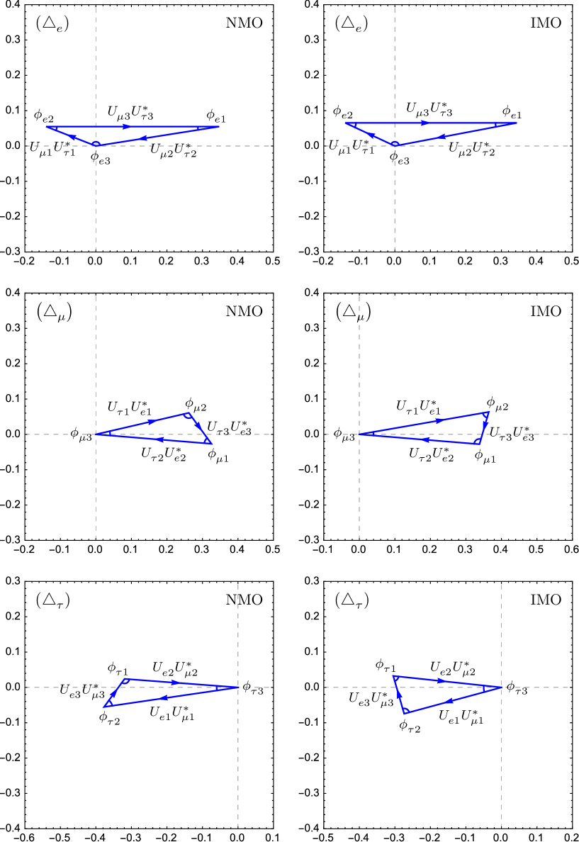
Figure 1: The real shapes of three Dirac UTs in the complex plane, plotted by inputting the best-fit values of $\theta_{12}$, $\theta_{13}$, $\theta_{23}$ and $\delta$ [12] in the NMO (left panel) or IMO (right panel) case.

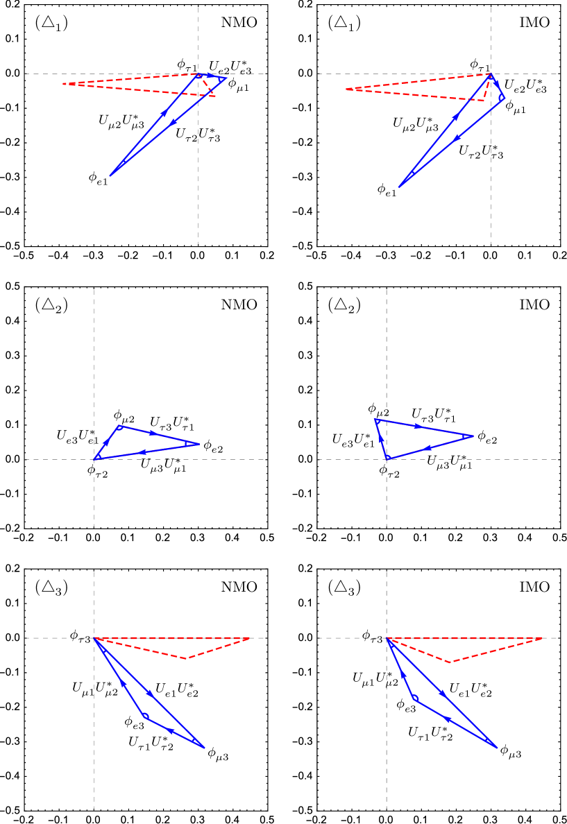
Figure 2: The real shapes and orientations of three Majorana UTs in the complex plane, plotted by assuming the Majorana phases $\left(\rho,\sigma\right)=\left(0,\pi/4\right)$ and inputting the best-fit values of $\theta_{12}$, $\theta_{13}$, $\theta_{23}$ and $\delta$ [12] in the NMO (left panel) or IMO (right panel) case. The dashed triangles correspond to $\left(\rho,\sigma\right)=\left(0,0\right)$ for comparison.

(a) In either the Dirac case or the Majorana case, the inner angles $\phi_{\mu 1}$ and $\phi_{\mu 2}$ (or $\phi_{\tau 1}$ and $\phi_{\tau 2}$) seem to be sensitive to the neutrino mass ordering. To understand this, we notice

$$\phi_{\tau 1}\simeq\phi_{\mu 2}\simeq\delta-\pi\;,\hskip 14.22636pt\phi_{\tau 2}\simeq\phi_{\mu 1}\simeq 2\pi-\delta\;$$ (6)

in the leading-order approximation thanks to the relative smallness of $\theta_{13}$. Hence these four angles are actually sensitive to the best-fit value of $\delta$, which belongs to the third quadrant in the NMO case (i.e., $\Delta m^{2}_{31}>0$) or the second quadrant in the IMO case (i.e., $\Delta m^{2}_{32}<0$) as given above. In comparison, the other five inner angles of the UTs are not so sensitive to $\delta$, and thus their results do not drastically change in the NMO and IMO cases, as one can easily see in Figures 1 and 2.

(b) The so-called Jarlskog invariant of the $3\times 3$ PMNS matrix $U$ [21] is now given as

$${\cal J}=\sin 2\theta_{12}\cos\theta_{13}\sin 2\theta_{13}\sin 2\theta_{23}\frac{\sin\delta}{8}\simeq\displaystyle\left\{\begin{array}[]{l}-2.68\times 10^{-2}\hskip 14.22636pt({\rm NMO})\;,\\ -3.16\times 10^{-2}\hskip 14.22636pt({\rm IMO})\;,\end{array}\right.$$ (9)

and it measures the strength of CP violation in neutrino oscillations. In particular, all the areas of the six different UTs are equal to $|{\cal J}|/2$ [2]. On the other hand, the nine inner angles of these triangles may form the following angle matrix:

$$\Phi=\begin{pmatrix}\phi_{e1}&\phi_{e2}&\phi_{e3}\cr\phi_{\mu 1}&\phi_{\mu 2}&\phi_{\mu 3}\cr\phi_{\tau 1}&\phi_{\tau 2}&\phi_{\tau 3}\end{pmatrix}\simeq\displaystyle\left\{\begin{array}[]{l}\begin{pmatrix}9.00^{\circ}&21.44^{\circ}&149.56^{\circ}\cr 49.33^{\circ}&112.90^{\circ}&17.77^{\circ}\cr 121.67^{\circ}&45.66^{\circ}&12.67^{\circ}\end{pmatrix}\hskip 14.22636pt({\rm NMO})\;,\\ \begin{pmatrix}10.79^{\circ}&\hskip 2.27626pt25.11^{\circ}\hskip 2.27626pt&144.10^{\circ}\cr 101.31^{\circ}&64.11^{\circ}&14.58^{\circ}\cr 67.90^{\circ}&90.78^{\circ}&21.32^{\circ}\end{pmatrix}\hskip 14.22636pt({\rm IMO})\;,\end{array}\right.$$ (12)

whose elements satisfy the sum rules $\phi_{\alpha 1}+\phi_{\alpha 2}+\phi_{\alpha 3}=\phi_{ei}+\phi_{\mu i}+\phi_{\tau i}=\pi$ (for $\alpha=e,\mu,\tau$ and $i=1,2,3$) [8, 22]. We find that the two off-diagonal asymmetries of $\Phi$ about its $\phi_{e1}$–$\phi_{\mu 2}$–$\phi_{\tau 3}$ and $\phi_{e3}$–$\phi_{\mu 2}$–$\phi_{\tau 1}$ axes read as

$${\cal A}_{\rm L} \equiv \phi_{e2}-\phi_{\mu 1}=\phi_{\mu 3}-\phi_{\tau 2}=\phi_{\tau 1}-\phi_{e3}\simeq\left\{\begin{array}[]{l}-27.89^{\circ}\hskip 14.22636pt({\rm NMO})\;,\\ -76.20^{\circ}\hskip 14.22636pt({\rm IMO})\;;\end{array}\right.$$ (15)

$${\cal A}_{\rm R} \equiv \phi_{e2}-\phi_{\mu 3}=\phi_{\mu 1}-\phi_{\tau 2}=\phi_{\tau 3}-\phi_{e1}\simeq\left\{\begin{array}[]{l}+3.67^{\circ}\hskip 19.91684pt({\rm NMO})\;,\\ +10.53^{\circ}\hskip 14.22636pt({\rm IMO})\;.\end{array}\right.$$ (18)

These results mean that $\Phi$ only contains four independent elements, which can reversely be used to determine the Dirac CP-violating phase and three flavor mixing angles.

(c) The three Majorana UTs are more interesting in the sense that their orientations depend on the values of the phase parameters $\rho$ and $\sigma$. Even though the UTs collapsed into lines in the $\delta=0$ (or $\pi$) case, there would exist leptonic CP violation unless those lines happened to lie in the abscissa or ordinate axis. This point was first observed in Ref. [3], and it has been clearly illustrated in Figure 2 with the typical inputs $\rho=0$ and $\sigma=\pi/4$. In fact, the orientations of triangles $\triangle_{1}$, $\triangle_{2}$ and $\triangle_{3}$ depend respectively on $\sigma$, $-\rho$ and $\rho-\sigma$ in the chosen parametrization of $U$. That is why $\triangle_{2}$ keeps unchanged when the $(\rho,\sigma)=(0,0)$ case is shifted to the $(\rho,\sigma)=(0,\pi/4)$ case in our plotting. In general, the Majorana UTs $\triangle_{1}$, $\triangle_{2}$ and $\triangle_{3}$ with arbitrary values of $\rho$ and $\sigma$ can be obtained through rotating their counterparts with $\rho=\sigma=0$ anticlockwise by $\sigma$, $-\rho$ and $\rho-\sigma$, respectively.

(d) To reflect the Majorana nature of the PMNS matrix $U$, one may redefine the Majorana phases as follows: $\psi_{\alpha i}\equiv\arg\left(U_{\alpha j}U^{*}_{\alpha k}\right)$ with the Latin subscripts running over $(1,2,3)$ in a cyclic way. These phases are independent of the phases of three charged leptons, and they form the following phase matrix:

$$\Psi=\begin{pmatrix}\psi_{e1}&\psi_{e2}&\psi_{e3}\cr\psi_{\mu 1}&\psi_{\mu 2}&\psi_{\mu 3}\cr\psi_{\tau 1}&\psi_{\tau 2}&\psi_{\tau 3}\end{pmatrix}\simeq\displaystyle\left\{\begin{array}[]{l}\begin{pmatrix}-9.00^{\circ}&54.00^{\circ}&-45.00^{\circ}\cr 49.33^{\circ}&-171.66^{\circ}&122.33^{\circ}\cr-139.67^{\circ}&-13.10^{\circ}&152.77^{\circ}\end{pmatrix}\hskip 14.22636pt({\rm NMO})\;,\\ \begin{pmatrix}-61.00^{\circ}&\hskip 2.27626pt106.00^{\circ}\hskip 2.27626pt&-45.00^{\circ}\cr 51.10^{\circ}&-164.78^{\circ}&113.68^{\circ}\cr-139.69^{\circ}&-9.89^{\circ}&149.58^{\circ}\end{pmatrix}\hskip 14.22636pt({\rm IMO})\;,\end{array}\right.$$ (21)

where we have used the same inputs as those in obtaining Eq. (8), and taken $\rho=0$ and $\sigma=\pi/4$ for illustration. It is obvious that the nine elements in the three rows of $\Psi$ satisfy the sum rules $\psi_{\alpha 1}+\psi_{\alpha 2}+\psi_{\alpha 3}=0$ (for $\alpha=e,\mu,\tau$) [8], but those in the three columns do not have a definite correlation. Hence the number of independent parameters in $\Psi$ is six, two more as compared with that in $\Phi$. Given Eq. (5), the nine inner angles of the sixe UTs can be expressed in terms of the nine elements of $\Psi$ as

$$\phi_{\alpha i}=\psi_{\beta i}-\psi_{\gamma i}\pm\pi\;,$$ (22)

in which the Greek subscripts run over $(e,\mu,\tau)$ cyclically, and the “$\pm$” sign should be taken in a proper way to assure $\phi_{\alpha i}\in\left[0,\pi\right)$.

The numerical results for the shapes and inner angles of $\triangle_{\alpha}$ (for $\alpha=e,\mu,\tau$) and $\triangle_{i}$ (for $i=1,2,3$) given above are subject to the inputs of the best-fit values of $\theta_{12}$, $\theta_{13}$, $\theta_{23}$ and $\delta$. Among them, $\delta$ involves the largest uncertainty. One may fix the values of the three flavor mixing angles to check how the shapes of six UTs change with different values of $\delta$. Instead of making such a check by taking some numerical examples, let us outline a general observation based on the leading-order analytical approximations made in Eq. (6). It is clear how $\phi_{\tau 1}\simeq\phi_{\mu 2}\simeq\delta-\pi$ and $\phi_{\tau 2}\simeq\phi_{\mu 1}\simeq 2\pi-\delta$ vary with the change of $\delta$. Because $\phi_{\mu 1}+\phi_{\mu 2}\simeq\phi_{\mu 1}+\phi_{\tau 1}\simeq\phi_{\tau 1}+\phi_{\tau 2}\simeq\phi_{\mu 2}+\phi_{\tau 2}\simeq\pi$ holds as a consequence of the above approximations, the inner angles $\phi_{e1}$, $\phi_{e2}$, $\phi_{\mu 3}$ and $\phi_{\tau 3}$ must be small as required by the unitarity conditions, and hence $\phi_{e3}$ must be the largest inner angle. This general analytical observation is actually supported by the explicit numerical results shown in Eq. (8).

When the uncertainties of all the four input parameters are taken into account, the situation will become quite messy. To illustrate, let us consider the $1\sigma$ intervals of the input quantities and calculate the nine inner angles of six UTs. As illustrated in Table 1, the $1\sigma$ uncertainty of each inner angle is rather significant as compared with its best-fit outcome, implying a remarkable change of the shape of each UT. A direct illustration of such uncertainties of $\triangle_{\alpha}$ and $\triangle_{i}$ in the complex plane is difficult, since all the sides and inner angles will deviate from those in the best-fit case (i.e., in Figures 1 and 2). At present one possible way out is to rescale and rotate each UT to make two of its three vertices always locate at the $(0,0)$ and $(1,0)$ points in the horizontal coordinate axis [12]. In this case, however, the uncertainty associated with the third vertex of each rescaled UT remains quite significant. Although the sides of each real UT and those of its rescaled counterpart are different, the inner angles of these two triangles are exactly the same. So Table 1 is almost equally helpful for illustrating how the shapes of six UTs are sensitive to the uncertainties of $\theta_{12}$, $\theta_{13}$, $\theta_{23}$ and especially $\delta$. Once $\delta$ is determined in the next-generation accelerator-based neutrino oscillation experiments, it will be possible for us to see the true shapes of leptonic UTs to a reasonably good degree of accuracy, just as we have seen the true shapes of six CKM UTs in the quark sector today .

Table 1: The numerical results for nine inner angles of the six UTs obtained with the inputs of the best-fit values and $1\sigma$ ranges of $\theta_{12}$, $\theta_{13}$, $\theta_{23}$ and $\delta$ [12]. Note that the unitarity conditions $\phi_{\alpha 1}+\phi_{\alpha 2}+\phi_{\alpha 3}=\phi_{ei}+\phi_{\mu i}+\phi_{\tau i}=\pi$ must hold (for $\alpha=e,\mu,\tau$ and $i=1,2,3$).

		Normal mass ordering (NMO)				Inverted mass ordering (IMO)
		best-fit		$\pm 1\sigma$ range		best-fit		$\pm 1\sigma$ range
$\phi_{e1}$		$9.00^{\circ}$		$2.73^{\circ}$ — $11.90^{\circ}$		$10.79^{\circ}$		$2.19^{\circ}$ — $12.03^{\circ}$
$\phi_{e2}$		$21.44^{\circ}$		$6.52^{\circ}$ — $26.81^{\circ}$		$25.11^{\circ}$		$5.47^{\circ}$ — $27.13^{\circ}$
$\phi_{e3}$		$149.56^{\circ}$		$142.00^{\circ}$ — $170.54^{\circ}$		$144.10^{\circ}$		$141.60^{\circ}$— $172.20^{\circ}$
$\phi_{\mu 1}$		$49.33^{\circ}$		$13.41^{\circ}$ — $119.42^{\circ}$		$103.31^{\circ}$		$39.53^{\circ}$ — $167.04^{\circ}$
$\phi_{\mu 2}$		$112.90^{\circ}$		$44.87^{\circ}$ — $161.11^{\circ}$		$64.11^{\circ}$		$9.87^{\circ}$ — $129.39^{\circ}$
$\phi_{\mu 3}$		$17.77^{\circ}$		$5.21^{\circ}$ — $22.03^{\circ}$		$14.58^{\circ}$		$2.78^{\circ}$— $17.52^{\circ}$
$\phi_{\tau 1}$		$121.67^{\circ}$		$51.34^{\circ}$ — $163.72^{\circ}$		$67.90^{\circ}$		$10.65^{\circ}$ — $132.77^{\circ}$
$\phi_{\tau 2}$		$45.66^{\circ}$		$12.13^{\circ}$ — $114.46^{\circ}$		$90.78^{\circ}$		$33.72^{\circ}$ — $164.48^{\circ}$
$\phi_{\tau 3}$		$12.67^{\circ}$		$3.66^{\circ}$ — $19.17^{\circ}$		$21.32^{\circ}$		$4.67^{\circ}$— $23.38^{\circ}$

An interesting question that one may ask is whether one of the Dirac or Majorana UTs can be a special triangle, such as the right triangle or the isosceles triangle. This question makes sense because there do exist two right UTs ($\triangle_{c}$ and $\triangle_{s}$) in the quark sector [7] as indicated by current experimental data. If one is only concerned about Figures 1 and 2 plotted by inputting the best-fit values of $\theta_{12}$, $\theta_{13}$, $\theta_{23}$ and $\delta$, then the Dirac triangle $\triangle_{\tau}$ and the Majorana triangle $\triangle_{2}$ can be regarded as the right triangles with $\phi_{\tau 2}$ being very close to $\pi/2$ in the IMO case. This point is also clear in Eq. (8), where $\phi_{\tau 2}\simeq 90.78^{\circ}$ has been given. If $\phi_{\tau 2}=\pi/2$ holds exactly, then one will be able to obtain the following correlation between the Dirac phase and three flavor mixing angles:

$$\cos\delta=-\cot\theta_{12}\tan\theta_{23}\sin\theta_{13}\;,$$ (23)

implying that $\delta$ must deviate from $3\pi/2$ (or equivalently, $-\pi/2$) to some extent and lies in the third quadrant. Such an interesting relation can be tested with much more accurate neutrino oscillation data to be achieved in the foreseeable future, especially after $\delta$ is experimentally determined or constrained.

From a model-building point of view, the $\mu$-$\tau$ reflection symmetry should be the simplest and most natural flavor symmetry behind the observed pattern of neutrino mixing [24, 25]. It predicts $\delta=3\pi/2$ and $\theta_{23}=\pi/4$, and therefore one is left with $|U_{\mu i}|=|U_{\tau i}|$ (for $i=1,2,3$). In this special case, we find that the three Majorana triangles $\triangle_{i}$ turn out to be the isosceles triangles with $\phi_{\mu i}=\phi_{\tau i}$ (for $i=1,2,3$). Such a possibility is not consistent with the best-fit results of current experimental data, as one can see in either Eq. (8) or Figure 2, but it cannot be excluded if the $2\sigma$ or $3\sigma$ results of a global fit is taken into account. In comparison with the Majorana triangles, the Dirac triangles are not sensitive to the $\mu$-$\tau$ reflection symmetry.

In Ref. [9] it has been pointed out that the inner angles of three Dirac UTs can directly be related to the probabilities of normal neutrino oscillations. Here let us establish the direct relations between the Majorana phases $\psi_{\alpha i}$ defined above Eq. (10) and the probabilities of neutrino-antineutrino oscillations given in Ref. [26]. The results are

$$P\left(\nu_{\alpha}\to\overline{\nu}_{\beta}\right) \equiv \frac{|K|^{2}}{E^{2}}\left[\sum_{i}m_{i}^{2}\left(S_{\gamma i}^{\rm D}\right)^{2}+2\sum_{i<j}m_{i}m_{j}S_{\alpha k}^{\rm M}S_{\beta k}^{\rm M}\cos\left(2\Delta_{ji}-\psi_{\alpha k}-\psi_{\beta k}\right)\right]\;,$$

$$P\left(\overline{\nu}_{\alpha}\to\nu_{\beta}\right) \equiv \frac{|\overline{K}|^{2}}{E^{2}}\left[\sum_{i}m_{i}^{2}\left(S_{\gamma i}^{\rm D}\right)^{2}+2\sum_{i<j}m_{i}m_{j}S_{\alpha k}^{\rm M}S_{\beta k}^{\rm M}\cos\left(2\Delta_{ji}+\psi_{\alpha k}+\psi_{\beta k}\right)\right]\;,\hskip 17.07182pt$$ (24)

where the subscripts $(\alpha,\beta,\gamma)$ run over $(e,\mu,\tau)$ cyclically, $K$ and $\overline{K}$ are the kinematical factors independent of the index $i$ (and they satisfy $|K|=|\overline{K}|$), $S^{\rm D}_{\alpha i}\equiv|U_{\beta i}U^{*}_{\gamma i}|$ defines one side of the Dirac UTs, $S^{\rm M}_{\alpha i}\equiv|U_{\alpha j}U^{*}_{\alpha k}|$ defines one side of the Majorana UTs with $(i,j,k)$ running over $(1,2,3)$ cyclically, and $\Delta_{ji}\equiv\Delta m^{2}_{ji}L/\left(4E\right)$ with $\Delta m^{2}_{ji}=m^{2}_{j}-m^{2}_{i}$. It is therefore clear that the difference between the probabilities of $\nu_{\alpha}\to\overline{\nu}_{\beta}$ and $\overline{\nu}_{\alpha}\to\nu_{\beta}$ oscillations,

$$P\left(\nu_{\alpha}\to\overline{\nu}_{\beta}\right)-P\left(\overline{\nu}_{\alpha}\to\nu_{\beta}\right)=4\frac{|K|^{2}}{E^{2}}\sum_{i<j}\left[m_{i}m_{j}S_{\alpha k}^{\rm M}S_{\beta k}^{\rm M}\sin\left(2\Delta_{ji}\right)\sin\left(\psi_{\alpha k}+\psi_{\beta k}\right)\right]\;,$$ (25)

results from the nontrivial values of the Majorana phases. On the other hand, the rates of $\nu_{i}\to\nu_{j}+\gamma$ decays in the rest frame of $\nu_{i}$ (for $m_{i}>m_{j}$) can be expressed as

$$\Gamma^{\rm(M)}_{\nu_{i}\to\nu_{j}+\gamma}=\frac{9\alpha_{\rm em}G_{\rm F}^{2}m_{i}^{2}}{2^{10}\pi^{4}M_{W}^{4}}\left(1-\frac{m_{j}^{2}}{m_{i}^{2}}\right)^{3}\left[\left(1+\frac{m_{j}^{2}}{m_{i}^{2}}\right)X-\frac{2m_{j}}{m_{i}}Y\right]\;,$$ (26)

where

$$X \equiv \sum_{\alpha}m_{\alpha}^{4}\left(S_{\alpha k}^{\rm M}\right)^{2}-\sum_{\alpha\neq\beta}m_{\alpha}^{2}m_{\beta}^{2}S_{\alpha k}^{\rm M}S_{\beta k}^{\rm M}\cos\left(\psi_{\alpha k}-\psi_{\beta k}\right)\;,$$

$$Y \equiv \sum_{\alpha}m_{\alpha}^{4}\left(S_{\alpha k}^{\rm M}\right)^{2}\cos\left(2\psi_{\alpha k}\right)+\sum_{\alpha\neq\beta}m_{\alpha}^{2}m_{\beta}^{2}S_{\alpha k}^{\rm M}S_{\beta k}^{\rm M}\cos\left(\psi_{\alpha k}+\psi_{\beta k}\right)\;$$ (27)

with $\alpha$ and $\beta$ running over $e$, $\mu$ and $\tau$. Since such decay modes are CP-conserving, their rates remain finite even if all the Majorana phases vanish.

Although both neutrino-antineutrino oscillations and neutrino decays are undetectable at present, Eqs. (13)—(16) show that their sensitivities to the Majorana UTs are conceptually interesting and thus deserve a careful study. Note that all the sides of the Dirac UTs (i.e., $S^{\rm D}_{\alpha i}$) can be determined from the appearance experiments of normal neutrino oscillations, and all the sides of the Majorana UTs (i.e., $S^{\rm M}_{\alpha i}$) are measurable in the disappearance experiments of normal neutrino oscillations [27]. Hence only the absolute neutrino mass scale and the CP-violating phases are still unknown in the probabilities of neutrino-antineutrino oscillations and the rates of neutrino decays shown above. If such rare processes can really be measured in the future, it will be greatly useful for probing the Majorana phases of massive neutrinos. In practice, the $0\nu 2\beta$ decay is the only LNV process that is being searched for in depth at low energies, and its effective neutrino mass can be expressed as

$$\left|\langle m\rangle_{ee}\right| = \displaystyle m_{2}|U_{e2}|^{2}\left|1+\frac{m_{1}}{m_{2}}\cdot\frac{U^{2}_{e1}}{U^{2}_{e2}}+\frac{m_{3}}{m_{2}}\cdot\frac{U^{2}_{e3}}{U^{2}_{e2}}\right|$$ (28)

$$= \displaystyle m_{2}|U_{e2}|^{2}\left|1+\frac{m_{1}}{m_{2}}\left|\frac{U_{e1}}{U_{e2}}\right|^{2}e^{+2{\rm i}\psi_{e3}}+\frac{m_{3}}{m_{2}}\left|\frac{U_{e3}}{U_{e2}}\right|^{2}e^{-2{\rm i}\psi_{e1}}\right|\;.$$

So a measurement of $|\langle m\rangle_{ee}|$ will allow us to constrain $\psi_{e1}$ and $\psi_{e3}$, but more experimental information from some other LNV processes is needed in order to fully determine these two Majorana phases in the standard three-flavor neutrino mixing scheme.

3 Effective MTs

Since the $3\times 3$ Majorana mass matrix totally involves six independent elements defined in Eq. (3), one may extend the exercise done in Eq. (17) to reexpress the effective Majorana mass terms $\langle m\rangle_{\alpha\beta}$ as follows:

$$\langle m\rangle_{\alpha\beta} = \displaystyle m_{2}U_{\alpha 2}U_{\beta 2}\left(1+\frac{m_{1}}{m_{2}}\cdot\frac{U_{\alpha 1}U_{\beta 1}}{U_{\alpha 2}U_{\beta 2}}+\frac{m_{3}}{m_{2}}\cdot\frac{U_{\alpha 3}U_{\beta 3}}{U_{\alpha 2}U_{\beta 2}}\right)$$ (29)

$$= \displaystyle m_{2}U_{\alpha 2}U_{\beta 2}\left[1+\frac{m_{1}}{m_{2}}\left|\frac{U_{\alpha 1}U_{\beta 1}}{U_{\alpha 2}U_{\beta 2}}\right|e^{+{\rm i}\left(\psi_{\alpha 3}+\psi_{\beta 3}\right)}+\frac{m_{3}}{m_{2}}\left|\frac{U_{\alpha 3}U_{\beta 3}}{U_{\alpha 2}U_{\beta 2}}\right|e^{-{\rm i}\left(\psi_{\alpha 1}+\psi_{\beta 1}\right)}\right]\;,\hskip 14.22636pt$$

where $\alpha$ and $\beta$ run over $e$, $\mu$ and $\tau$. In the complex plane Eq. (18) represents six quadrangles whose inner angles are some combinations of the Majorana phases. But such a geometrical description is so complicated that it might not be very useful for neutrino phenomenology. For this reason, we shall subsequently focus on a much simpler but interesting situation.

It is obvious that one of the two phase combinations in Eq. (18) can always be rotated away in the neutrino mass limit $m_{1}\to 0$ or $m_{3}\to 0$. Given the phase convention of the PMNS matrix $U$ in Eq. (4), one may simply switch off $\rho$ so as to fit the $m_{1}=0$ or $m_{3}=0$ case. For this reason, we write out the explicit expressions of the six effective Majorana neutrino masses defined in Eq. (3) by setting $\rho=0$:

$$\langle m\rangle_{ee} \equiv \displaystyle m_{1}c_{12}^{2}c_{13}^{2}+m_{2}s_{12}^{2}c_{13}^{2}e^{2{\rm i}\sigma}+m_{3}s_{13}^{2}e^{-2{\rm i}\delta}\;,$$

$$\langle m\rangle_{\mu\mu} \equiv \displaystyle m_{1}\left(s_{12}c_{23}+c_{12}s_{13}s_{23}e^{{\rm i}\delta}\right)^{2}+m_{2}\left(c_{12}c_{23}-s_{12}s_{13}s_{23}e^{{\rm i}\delta}\right)^{2}e^{2{\rm i}\sigma}+m_{3}c_{13}^{2}s_{23}^{2}\;,$$

$$\langle m\rangle_{\tau\tau} \equiv \displaystyle m_{1}\left(s_{12}s_{23}-c_{12}s_{13}c_{23}e^{{\rm i}\delta}\right)^{2}+m_{2}\left(c_{12}s_{23}+s_{12}s_{13}c_{23}e^{{\rm i}\delta}\right)^{2}e^{2{\rm i}\sigma}+m_{3}c_{13}^{2}c_{23}^{2}\;;$$

$$\langle m\rangle_{e\mu} \equiv \displaystyle-m_{1}c_{12}c_{13}\left(s_{12}c_{23}+c_{12}s_{13}s_{23}e^{{\rm i}\delta}\right)+m_{2}s_{12}c_{13}\left(c_{12}c_{23}-s_{12}s_{13}s_{23}e^{{\rm i}\delta}\right)e^{2{\rm i}\sigma}$$

$$\displaystyle+m_{3}c_{13}s_{13}s_{23}e^{-{\rm i}\delta}\;,$$

$$\langle m\rangle_{e\tau} \equiv \displaystyle m_{1}c_{12}c_{13}\left(s_{12}s_{23}-c_{12}s_{13}c_{23}e^{{\rm i}\delta}\right)-m_{2}s_{12}c_{13}\left(c_{12}s_{23}+s_{12}s_{13}c_{23}e^{{\rm i}\delta}\right)e^{2{\rm i}\sigma}$$

$$\displaystyle+m_{3}c_{13}s_{13}c_{23}e^{-{\rm i}\delta}\;,$$

$$\langle m\rangle_{\mu\tau} \equiv \displaystyle-m_{1}\left(s_{12}s_{23}-c_{12}s_{13}c_{23}e^{{\rm i}\delta}\right)\left(c_{23}s_{12}+c_{12}s_{13}s_{23}e^{{\rm i}\delta}\right)$$ (30)

$$\displaystyle-m_{2}\left(c_{12}s_{23}+s_{12}s_{13}c_{23}e^{{\rm i}\delta}\right)\left(c_{12}c_{23}-s_{12}s_{13}s_{23}e^{{\rm i}\delta}\right)e^{2{\rm i}\sigma}+m_{3}c_{13}^{2}c_{23}s_{23}\;.\hskip 11.38092pt$$

Then it is much easier to consider the $m_{1}\to 0$ or $m_{3}\to 0$ limit, in which $\langle m\rangle_{\alpha\beta}$ and its two component vectors form a mass triangle (MT) in the complex plane.

In view of the best-fit values of two neutrino mass-squared differences reported by Gonzalez-Garcia et al [11], we obtain $m_{2}\simeq 0.0087$ eV and $m_{3}\simeq 0.0496$ eV in the $m_{1}\to 0$ limit (NMO); or $m_{1}\simeq 0.0487$ eV and $m_{2}\simeq 0.0495$ eV in the $m_{3}\to 0$ limit (IMO). In either case one may plot the six effective MTs with the help of Eq. (16), the best-fit values of $\theta_{12}$, $\theta_{13}$, $\theta_{23}$ and $\delta$, and the assumption of $\sigma=\pi/4$. Our results about the MTs $\triangle A_{i}B_{i}C_{i}$ (for $i=1,2,\cdots,6$, NMO) or $\triangle D_{i}E_{i}F_{i}$ (for $i=1,2,\cdots,6$, IMO) are shown in Figures 3 and 4, respectively. Some discussions and comments are in order.

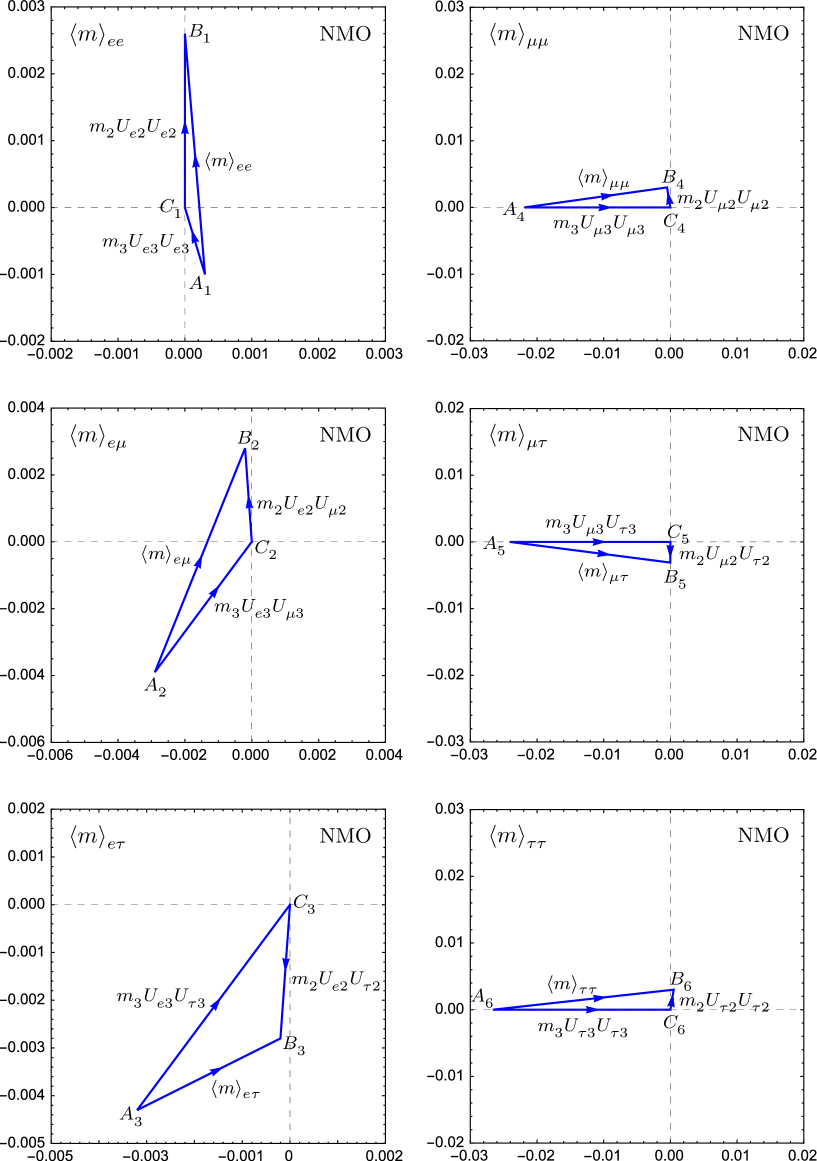
Figure 3: Six effective MTs $\triangle A_{i}B_{i}C_{i}$ (for $i=1,2,\cdots,6$) of the Majorana neutrinos in the $m_{1}\to 0$ limit in the complex plane, plotted by assuming the Majorana phase $\sigma=\pi/4$ and inputting the best-fit values of $\Delta m^{2}_{21}$, $\Delta m^{2}_{31}$, $\theta_{12}$, $\theta_{13}$, $\theta_{23}$ and $\delta$ [12] in the NMO case.

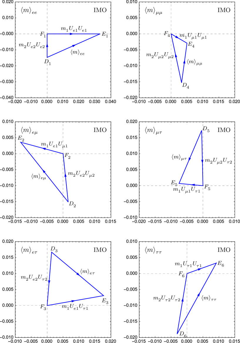
Figure 4: Six effective MTs $\triangle D_{i}E_{i}F_{i}$ (for $i=1,2,\cdots,6$) of the Majorana neutrinos in the $m_{3}\to 0$ limit in the complex plane, plotted by assuming the Majorana phase $\sigma=\pi/4$ and inputting the best-fit values of $\Delta m^{2}_{21}$, $\Delta m^{2}_{32}$, $\theta_{12}$, $\theta_{13}$, $\theta_{23}$ and $\delta$ [12] in the IMO case.

(1) A remarkable merit of these effective MTs is that they allow us to easily read off the magnitudes of $\langle m\rangle_{\alpha\beta}$. For instance, $|\langle m\rangle_{ee}|\sim|\langle m\rangle_{e\mu}|\sim|\langle m\rangle_{e\tau}|\sim{\cal O}\left(10^{-3}\right)$ eV and $|\langle m\rangle_{\mu\mu}|\sim|\langle m\rangle_{\mu\tau}|\sim|\langle m\rangle_{\tau\tau}|\sim{\cal O}\left(10^{-2}\right)$ eV in the NMO case; or $|\langle m\rangle_{\alpha\beta}|\sim{\cal O}\left(10^{-2}\right)$ eV in the IMO case. Because of $m_{2}/m_{3}\simeq 17.5\%$ in the $m_{1}\to 0$ limit, it is easy to understand why the shortest side of $\triangle A_{4}B_{4}C_{4}$ is $m_{2}|U_{\mu 2}|^{2}$ and why $|\langle m\rangle_{\mu\mu}|\simeq m_{3}|U_{\mu 3}|^{2}$ holds. The effective MTs $\triangle A_{5}B_{5}C_{5}$ and $\triangle A_{6}B_{6}C_{6}$ have a similar property in the NMO case. In comparison, the $m_{3}\to 0$ case is simpler because $|\langle m\rangle_{\alpha\beta}|\propto m_{2}\simeq m_{3}$ holds.

(2) In the IMO case the effective MT $\triangle D_{1}E_{1}F_{1}$ is especially interesting because its inner angle $\angle D_{1}F_{1}E_{1}$ happens to equal $2\sigma$ thanks to $m_{3}\to 0$. Therefore, a measurement of $|\langle m\rangle_{ee}|$ of the $0\nu 2\beta$ decay will allow one to determine the Majorana phase $\sigma$ in the $m_{3}\to 0$ limit. Similarly, $\angle A_{5}C_{5}B_{5}\simeq 2\sigma$ holds in the $m_{1}\to 0$ limit thanks to the smallness of $\theta_{13}$. This observation implies that it is possible to determine the Majorana phase from a measurement of the effective mass $|\langle m\rangle_{\mu\tau}|$ in the NMO case with $m_{1}\simeq 0$.

(3) The texture of the symmetric Majorana neutrino mass matrix $M_{\nu}$, whose six independent elements are just equal to $\langle m\rangle_{\alpha\beta}$ (for $\alpha,\beta=e,\mu,\tau$), can be illustrated with the help of Figures 3 and 4 as follows:

$$|M_{\nu}|=\begin{pmatrix}|\langle m\rangle_{ee}|&|\langle m\rangle_{e\mu}|&|\langle m\rangle_{e\tau}|\cr|\langle m\rangle_{e\mu}|&|\langle m\rangle_{\mu\mu}|&|\langle m\rangle_{\mu\tau}|\cr|\langle m\rangle_{e\tau}|&|\langle m\rangle_{\mu\tau}|&|\langle m\rangle_{\tau\tau}|\cr\end{pmatrix}\simeq\displaystyle\left\{\begin{array}[]{l}\begin{pmatrix}0.0036&0.0072&0.0033\cr 0.0072&0.0217&0.0243\cr 0.0033&0.0243&0.0273\end{pmatrix}\hskip 14.22636pt(m_{1}\to 0)\;,\\ \begin{pmatrix}0.0363&0.0239&0.0213\cr 0.0239&0.0125&0.0180\cr 0.0213&0.0180&0.0254\cr\end{pmatrix}\hskip 14.22636pt(m_{3}\to 0)\;,\end{array}\right.$$ (33)

in unit of eV. Such a texture of $M_{\nu}$ may be reproduced in a specific neutrino mass model once a kind of flavor symmetry and its proper breaking are taken into account [28].

Note that the probabilities of neutrino-antineutrino oscillations given in Eq. (13) can be simplified to

$$P\left(\nu_{\alpha}\to\overline{\nu}_{\beta}\right)=P\left(\overline{\nu}_{\alpha}\to\nu_{\beta}\right)=\frac{|K|^{2}}{E^{2}}\left|\langle m\rangle_{\alpha\beta}\right|^{2}\;$$ (34)

in the $L\to 0$ limit (i.e., the so-called zero-distance effect). This result is a clear reflection of the Majorana nature of massive neutrinos. In fact, the effective Majorana neutrino masses $\langle m\rangle_{\alpha\beta}$ may also show up in some other LNV processes, such the $H^{++}\to\alpha^{+}\beta^{+}$ decays in the type-II seesaw mechanism [29]. The branching ratios of these decay modes are

$${\cal B}(H^{++}\to\alpha^{+}\beta^{+})=\frac{2}{1+\delta_{\alpha\beta}}\cdot\frac{\left|\langle m\rangle_{\alpha\beta}\right|^{2}}{\displaystyle m^{2}_{1}+m^{2}_{2}+m^{2}_{3}}\;,$$ (35)

where $\alpha$ and $\beta$ run over $e$, $\mu$ and $\tau$. In the limit of $m_{1}\to 0$ or $m_{3}\to 0$, one may calculate ${\cal B}(H^{++}\to\alpha^{+}\beta^{+})$ by inputting the best-fit values of relevant neutrino oscillation parameters and allowing the Majorana phase $\sigma$ to vary from $0$ to $2\pi$. The numerical results are listed in Table 2 for the sake of illustration. Compared with the previous estimates of such decay modes made some years ago [30], our present results are more convergent because today’s neutrino oscillation data are more accurate and the neutrino mass limit under consideration is very special. Of course, whether the type-II seesaw mechanism really works in Nature remains an open question, and how to measure possible rare LNV processes is a very big experimental challenge. The point that we are stressing is to see a potential link between the effective Majorana neutrino masses and some interesting LNV phenomena.

Table 2: The expected branching ratios of $H^{++}\to\alpha^{+}\beta^{+}$ decays in the type-II seesaw mechanism, where the best-fit values of $\Delta m^{2}_{21}$, $\Delta m^{2}_{31}$ (or $\Delta m^{2}_{32}$), $\theta_{12}$, $\theta_{13}$, $\theta_{23}$ and $\delta$ [12] have been input and $\sigma\in[0,2\pi)$ has been taken.

Branching ratios	In the $m_{1}\to 0$ limit	In the $m_{3}\to 0$ limit
${\cal B}(H^{++}\to e^{+}e^{+})$	$0.0894\%\to 0.5307\%$	$7.0476\%\to 47.5258\%$
${\cal B}(H^{++}\to e^{+}\mu^{+})$	$0.3426\%\to 4.6215\%$	$0.0744\%\to 34.8293\%$
${\cal B}(H^{++}\to e^{+}\tau^{+})$	$0.5022\%\to 5.3036\%$	$0.0613\%\to 50.2589\%$
${\cal B}(H^{++}\to\mu^{+}\mu^{+})$	$14.1339\%\to 24.5069\%$	$2.0129\%\to 9.4731\%$
${\cal B}(H^{++}\to\mu^{+}\tau^{+})$	$35.0848\%\to 58.3642\%$	$3.9764\%\to 25.5264\%$
${\cal B}(H^{++}\to\tau^{+}\tau^{+})$	$21.7296\%\to 34.7906\%$	$1.8257\%\to 17.3884\%$

Assuming that a positive signal of the $0\nu 2\beta$ decay can be measured someday, then the corresponding knowledge of $|\langle m\rangle_{ee}|$ will allow one to predict the rates of some other rare LNV processes, such as $P(\nu_{e}\to\overline{\nu}_{e})=|K|^{2}|\langle m\rangle_{ee}|^{2}/E^{2}$ from Eq. (21) and ${\cal B}(H^{++}\to e^{+}e^{+})=|\langle m\rangle_{ee}|^{2}/\left(m^{2}_{1}+m^{2}_{2}+m^{2}_{3}\right)$ from Eq. (22). Once such a breakthrough really happens, it will definitely open a new window towards the deep secrets of Majorana particles.

4 Summary

Neutrino physics has entered the era of precision measurements, in which one is doing the best one can to answer some important questions, including what the absolute neutrino mass scale is, whether massive neutrinos are the Majorana particles, how large the effects of leptonic CP violation can be, and so on. Before these questions are experimentally answered, one may theoretically or phenomenologically try every shift available to bridge the gap between the observable quantities and the fundamental flavor parameters in the neutrino sector. In this regard we have paid particular attention to an intuitive description of leptonic CP violation and effective Majorana neutrino masses in the complex plane — namely, the Dirac and Majorana UTs as well as the effective MTs in the $m_{1}\to 0$ or $m_{3}\to 0$ limit.

With the help of the best-fit values of neutrino oscillation parameters, we have plotted the six UTs of the PMNS matrix to show their real shapes in the complex plane. The connections of the Majorana UTs with neutrino-antineutrino oscillations and neutrino decays have been explored, and the possibilities of right or isosceles UTs have also been discussed. In the second part of this paper, we have considered a special but phenomenologically allowed neutrino mass spectrum with $m_{1}=0$ or $m_{3}=0$ and the corresponding effective Majorana neutrino masses $\langle m\rangle_{\alpha\beta}$ — the latter can form six MTs in the complex plane. In this case we have shown how these MTs look like by assuming the Majorana phase $\sigma$ to be $\pi/4$ as a typical example. The relations of such triangles to the LNV decays $H^{++}\to\alpha^{+}\beta^{+}$ in the type-II seesaw mechanism have been illustrated too.

We hope that this kind of study may enrich the neutrino phenomenology to some extent. Although the UTs and MTs can only provide us with a geometrical language to describe the flavor issues of massive neutrinos, they do have made some underlying physics more transparent and intuitive. So they are useful and interesting, and their phenomenological applications deserve some further exploration.

This work was supported in part by the National Natural Science Foundation of China under grant No. 11135009 and No. 11375207.

References

[1] N. Cabibbo, Phys. Rev. Lett. 10, 531 (1963); M.
Kobayashi and T. Masakwa, Prog. Theor. Phys. 49, 652 (1973).
[2] H. Fritzsch and Z.Z. Xing,
Prog. Part. Nucl. Phys. 45, 1 (2000) [arXiv:hep-ph/9912358].
[3] J.A. Aguilar-Saavedra and G.C. Branco,
Phys. Rev. D 62, 096009 (2000) [arXiv:hep-ph/0007025]
[4] J. Sato, Nucl. Instrum. Methods Phys. Res.,
Sect. A 472, 434 (2001); Y. Farzan and A.Yu. Smirnov,
Phys. Rev. D 65, 113001 (2002).
[5] Z.Z. Xing, Int. J. Mod. Phys. A 19,
1 (2004); H. Zhang and Z.Z. Xing, Eur. Phys. J. C
41, 143 (2005); Z.Z. Xing and H. Zhang, Phys. Lett. B
618, 131 (2005).
[6] Y. Koide, arXiv:hep-ph/0502054; S. Antusch,
C. Biggio, E. Fernandez-Martinez, M.B. Gavela, and J. Lopez-Pavon,
JHEP 0610, 084 (2006); J.D. Bjorken, P.F. Harrison, and W.G.
Scott, Phys. Rev. D 74, 073012 (2006); G. Ahuja and M. Gupta,
Phys. Rev. D 77, 057301 (2008); A. Dueck, S. Petcov, and W.
Rodejohann, Phys. Rev. D 82, 013005 (2010); P.S. Bhupal Dev,
C.H. Lee, and R.N. Mohapatra, Phys. Rev. D 88, 093010 (2013).
[7] Z.Z. Xing, Phys. Lett. B 679, 111 (2009).
[8] S. Luo, Phys. Rev. D 85, 013006 (2012).
[9] H.J. He and X.J. Xu, Phys. Rev. D 89, 073002 (2014).
[10] Y.F. Wang and Z.Z. Xing, arXiv:1504.06155.
[11] F. Capozzi, G.L. Fogli, E. Lisi, A. Marrone,
D. Montanino, and A. Palazzo, Phys. Rev. D 89, 093018 (2014).
[12] M.C. Gonzalez-Garcia, M. Maltoni, and T. Schwetz,
JHEP 1411, 052 (2014).
[13] K. Abe et. al. (T2K Collaboration), Phys. Rev.
Lett. 111, 211803 (2013); Phys. Rev. Lett. 112, 181801
(2014).
[14] F.P. An et. al. (Daya Bay Collaboration),
Phys. Rev. Lett. 112, 061801 (2014); Phys. Rev. Lett. 115, 111802 (2015).
[15] The latest global analysis can be found in: F. Capozzi,
E. Lisi, A. Marrone, D. Montanino and A. Palazzo, arXiv:1601.07777.
[16] B. Pontecorvo, Sov. Phys. JETP 6, 429 (1957);
Z. Maki, M. Nakagawa, and S. Sakata, Prog. Theor.
Phys. 28, 870 (1962); B. Pontecorvo, Sov. Phys. JETP 26,
984 (1968).
[17] Z.Z. Xing and Y.L. Zhou, Chin. Phys. C 39,
1 (2015).
[18] Z.Z. Xing and Y.L. Zhou, Mod. Phys. Lett. A 30,
1530019 (2015).
[19] K. Harigaya, M. Ibe, and T. Yanagida, Phys. Rev.
D 86, 013002 (2012); T. Yanagida, Nucl. Phys. Proc. Suppl.
235–236, 245 (2013).
[20] P.H. Frampton, S.L. Glashow, and T. Yanagida,
Phys. Lett. B 548, 119 (2002). For a review with extensive
references, see: W.L. Guo, Z.Z. Xing, and S. Zhou, Int. J. Mod.
Phys. E 16, 1 (2007); J. Zhang and S. Zhou, JHEP 1509,
065 (2015).
[21] C. Jarlskog, Phys. Rev. Lett. 55, 1039 (1985);
D.D. Wu, Phys. Rev. D 33, 860 (1986).
[22] In the quark sector the similar angle matrix of
the CKM matrix has been discussed. See, e.g., P.F. Harrison,
S. Dallison, and W.G. Scott, Phys. Lett. B 680, 328 (2009);
S. Luo and Z.Z. Xing, J. Phys. G 37, 075018 (2010).
[23] K.A. Olive et al. (Particle Data Group), Chin.
Phys. C 38, 090001 (2004) and 2015 update.
[24] Z.Z. Xing and S. Zhou, Phys. Lett. B 737,
196 (2014); S. Luo and Z.Z. Xing, Phys. Rev. D 90, 073005 (2014).
[25] For a review of the - flavor symmetry with
extensive references, see:
Z.Z. Xing and Z.H. Zhao, arXiv:1512.04207.
[26] Z.Z. Xing, Phys. Rev. D 87, 053019 (2013);
Z.Z. Xing and Y.L. Zhou, Phys. Rev. D 88, 033002 (2013).
[27] Z.Z. Xing and J.Y. Zhu, arXiv:1603.02002; J.Y. Zhu,
in preparation.
[28] See, e.g., G. Altarelli and F. Feruglio,
Rev. Mod. Phys. 82, 2701 (2010); S.F. King and C. Luhn,
Rept. Prog. Phys. 76, 056201 (2013).
[29] W. Konetschny and W. Kummer, Phys. Lett. B 70, 433
(1977); M. Magg and C. Wetterich, Phys. Lett. B 94, 61 (1980);
J. Schechter and J.W.F. Valle, Phys. Rev. D 22, 2227 (1980);
T.P. Cheng and L.F. Li, Phys. Rev. D 22, 2860 (1980).
[30] See, e.g., J. Garayoa and T. Schwetz, JHEP 0803, 009
(2008); M. Kadastik, M. Raidal, and L. Rebane, Phys. Rev. D 77, 115023 (2008); A.G. Akeroyd, M. Aoki, and H. Sugiyama, Phys.
Rev. D 77, 075010 (2008); P. Fileviez Perez, T. Han, G.Y.
Huang, T. Li, and K. Wang, Phys. Rev. D 78, 015018 (2008); P.
Ren and Z.Z. Xing, Phys. Lett. B 666, 48 (2008); Z.Z. Xing,
Phys. Rev. D 78, 011301 (2008).