Causality studied in reconstructed state space.
Examples of uni-directionally connected chaotic systems

Abstract

Three state-space based methods were tested in relation to the ability to detect unidirectional coupling and synchronization of interconnected dynamical systems. The first method, based on measure named M, was introduced by Andrzejak et al. in 2003 [1]. The second one, based on measure L, was described in 2009 by Chicharro et al. [5]. The third method, called convergent cross-mapping, came from Sugihara et al., 2012 [28].

The methods were compared on 9 test examples of uni-directionally connected chaotic systems of Hénon, Rössler and Lorenz type. The tested systems were selected from previously published causality studies. Matlab code for the three methods is provided.

The results show that each of the three examined state-space methods managed to reveal the presence and the direction of couplings and also to detect the onset of full synchronization.

Keywords: Causality, Synchronization, Unidirectional bivariate coupling, Hénon, Rössler, Lorenz, Correlation dimension, Cross-mapping

Institute of Measurement Science, Slovak Academy of Sciences,

Dúbravská Cesta 9, 842 19 Bratislava, Slovakia

E-mail address: krakovska@savba.sk

1 Introduction

Nowadays, the study of drive-response relationships between dynamical systems is a topic of increasing interest. Applications are found, among others, in domains as economics, climatology, electrical activity of brain, or cardio-respiratory relations.

In this paper examples of the next type of uni-directionally coupled bivariate dynamical systems are studied:

$\dot{x}(t)=F(x(t))$

$\dot{y}(t)=G(y(t),x(t))$

where $x$ and $y$ are state vectors of driving system $X$ and the driven response $Y$. If the following relation $y(t)=\text{$\Psi$}(x(t))$ applies for some smooth and invertible function $\Psi$ then there is said to be a generalized synchronization between $X$ and $Y$. If $\Psi$ is an identity, the synchronization is called identical. After some definitions, $\Psi$ does not need to be smooth. E.g., Pyragas defines as strong and weak synchronizations the cases of smooth and non-smooth transformations, respectively [20].

The direction of coupling can only be uncovered when the coupling is weaker than the threshold for an emergence of synchronization. Once the systems are synchronized, the future states of the driver $X$ can be predicted from the response $Y$ equally well as vice versa.

A first mathematical approach to detect causal relationships has been proposed in 1969 by Clive Granger [7]. The method was based on the premiss that causality could be reflected by measuring the ability of predicting the future values of a time series using past values of the driving time series. More specifically, a time series $X$ is said to cause $Y$ if it can be shown, usually through statistical hypothesis tests, that past $X$ values provide statistically significant information about future values of $Y$.

To be able to consider Granger causality (GC), separability is required. Namely, information about the causative factor $X$ is expected to be available as an explicit variable. This requirement can be problematic in a case of variables which are dynamically linked and sharing the same manifold in the state space.

Moreover, the initially linear concept requires generalizations to enable investigation of complex nonlinear processes. Therefore, new approaches were proposed, including nonlinear Granger causality, transfer entropy, cross predictability, conditional mutual information, measures evaluating distances of conditioned neighbors in reconstructed state spaces, etc.

In this study, we are going to focus on testing uni-directionally coupled chaotic systems by state-space methods.

The possibility to study synchronization in chaotic systems was discussed already in 1990 [19]. The problem with chaos is the long-term unpredictable behavior. Two identical chaotic systems starting at very close initial conditions soon diverge from each other, while remaining on the same attractor. However, although it may sound surprising, it is possible to “lock” one chaotic system to the other to get them to synchronize. Our test data will include several examples of such synchronized chaos.

In the case of the state-space methods, efforts to reveal causal links are based on the following idea. When trajectories of driving and response systems are strongly connected, then two close states in the state space of the response system correspond to two close states in the space of the driving system. Already in 1995, this approach was used by Rulkov et al. to explore systems where an observable of response system $y(t)$ is driven with the output of an autonomous driving system $x(t)$, but there is no feedback to the driver [24]. To investigate the existence of the synchronization the authors introduced the idea of mutual false nearest neighbors to determine when closeness in response space implies closeness in driving space. Similar idea was applied in a variety of modifications many times since then. Some of them will be presented below.

The paper is organized as follows.

In Section 2, the methods of causality detection are presented.

Section 3 describes the nine examples of uni-directionally coupled chaotic systems. At the same place the results of the causality detection are given for each case.

In Section 4, the findings are summarized.

In Appendix, Matlab code used for the detection of causality is provided. The program includes all three testing methods used in this study, namely measure $M$, measure $L$, and the cross-mapping.

2 Data and methods

2.1 Data

Our data set consists of 9 examples of chaotic systems of Hénon, Rössler and Lorenz type that are coupled with variable coupling strengths. Details on systems are provided in section 3.

Next, we briefly introduce the existing causality methods:

2.2 Granger test

When looking for causality, as first the test of Granger causality is usually applied [7]. For this purpose, freely available Matlab function written by Chandler Lutz [15] can be used, for example. However, in cases of non-separable non-linear dynamic systems, the Granger test fails to reliably detect and characterize the causal relations.

2.3 Transfer entropy and conditional mutual information

Although we will concentrate on state-space based approaches, for completeness let us mention the methods that originate in information theory. However, they will not be tested in the present study.

Transfer entropy (TE)

Transfer entropy was introduced by Schreiber [26] in 2000 as an information theoretic measure which shares some of the desired properties of mutual information but takes the dynamics of information transport into account. The definition is as follows

$$TE_{Y\to X} =\sum_{x_{t},x_{t-\tau}^{(k)},y_{t-\tau}^{(l)}}p(x_{t},x_{t-\tau}^{(k)},y_{t-\tau}^{(l)})\log\frac{p(x_{t}|x_{t-\tau}^{(k)},y_{t-\tau}^{(l)})}{p(x_{t}|x_{t-\tau}^{(k)})}$$

$$=H(x_{t},x_{t-\tau}^{(k)})-H(x_{t}|y_{t-\tau}^{(l)},x_{t-\tau}^{(k)})$$

where $H$ is the Shannon entropy, $t$ indicates a given point in time, $\tau$ is a time lag (usually the same time lag is used in both $X$ and $Y$) and $k$ and $l$ are the block lengths of past values in $X$ and $Y$.

$$x_{t-\tau}^{(k)} =\{y_{t-\tau-k+1},y_{t-\tau-k+2},...,y_{t-\tau}\}$$

$$y_{t-\tau}^{(l)} =\{y_{t-\tau-l+1},y_{t-\tau-l+2},...,y_{t-\tau}\}$$

Mostly, $l=k=1$, so we get

$$x_{t-\tau}^{(1)} =\{y_{t-\tau-1+1}\}$$

$$y_{t-\tau}^{(1)} =\{y_{t-\tau-1+1}\}$$

$$TE_{Y\to X} =\sum_{x_{t},x_{t-\tau},y_{t-\tau}}p(x_{t},x_{t-\tau},y_{t-\tau})\log\frac{p(x_{t}|x_{t-\tau},y_{t-\tau})}{p(x_{t}|x_{t-\tau})}$$

$$=H(x_{t},x_{t-\tau})-H(x_{t}|y_{t-\tau},x_{t-\tau}).$$

Conditional mutual information

Transfer entropy has been independently formulated as a conditional mutual information by Paluš et al. [18]. The joint entropy is defined as $H(X,Y)=-\sum\sum p(x,y)\,log\,p(x,y)$ and the conditional entropy is $H(Y|X)=-\sum\sum p(x,y)\,log\,p(y|x)$. Then the mutual information $I(X;Y)$ is defined as $I(X;Y)=H(X)+H(Y)-H(X,Y)$. The conditional mutual information of the variables $X,Y$, given the variable $Z$ is defined as the reduction in the uncertainty of $X$ due to knowledge of $Y$ when $Z$ is given:

$$I(X;Y|Z)=H(X|Z)+H(Y|Z)-H(X,Y|Z).$$

For $Z$ independent of $X$ and $Y$:

$I(X;Y|Z)=I(X;Y)=I(X;Y;Z)-I(X;Z)-I(Y;Z)$.

After the next substitution

$$x_{t-\tau}^{(k)} =Z$$

$$x_{t} =X$$

$$y_{t-\tau}^{(l)} =Y,$$

and following simple probability relations it turns out that the conditional mutual information $I(X;Y|Z)$ and the transfer entropy $TE$ are the same:

$$TE_{Y\to X} =H(X,Z)-H(X|Y,Z)=\sum_{X,Y,Z}p(X,Y,Z)\log\frac{p(X|Y,Z)}{p(X|Y)}$$

$$TE_{Y\to X} =\sum_{X,Y,Z}p(X,Y,Z)\log\frac{p(X|Y,Z)}{p(X|Z)}\frac{p(Y|Z)}{p(Y|Z)}=\sum_{X,Y,Z}p(X,Y,Z)\log\frac{p(X,Y|Z)}{p(X|Z)p(Y|Z)}$$

$$=\sum_{X,Y,Z}p(X,Y,Z)\log p(X,Y|Z)-\sum_{X,Y,Z}p(X,Y,Z)\log p(X|Z)$$

$$-\sum_{X,Y,Z}p(X,Y,Z)\log p(Y|Z)$$

$$=\sum_{X,Y,Z}p(X,Y,Z)\log p(X,Y|Z)-\sum_{X,Z}p(X,Z)\log p(X|Z)-\sum_{Y,Z}p(Y,Z)\log p(Y|Z)$$

$$=-H(X,Y|Z)+H(X|Z)+H(Y|Z)=I(X;Y|Z)$$

In [4] Barnett et al. have shown that for Gaussian variables, Granger causality and transfer entropy (conditional mutual information) are equivalent.

2.4 Correlation dimension

In this study, we tested two aspects of causality. First of all we tested the ability to detect the presence and direction of the causal link for a particular value of coupling. Secondly, we would like to be able to detect a possible onset of synchronization following an increase of coupling above a certain value. Therefore, we need to know which levels of coupling lead to synchronization for our artificial chaotic systems. Typically, to this end, the Lyapunov exponents are evaluated, as it was shown that the synchronization takes place when all of the conditional Lyapunov exponents of the response subsystem become negative.

However, in this study, similarly as in [11] we use a different complexity measure, namely the correlation dimension, computed after Grassberger-Proccacia algorithm [8] to reveal the emergence of synchronization. The idea behind this approach is as follows.

Suppose we have a driving system $X$ and response $Y$ with a unidirectional coupling. Let us create $X+Y$ combining state vectors of $X$ and $Y$. Then, we have the next expectations with regard to the coupling effects on the correlation dimension:

- for uncoupled $X$ and $Y$ the correlation dimension of the combined system are equal to the sum of the dimensions of $X$ and $Y$,

- for coupled but not synchronized case, the correlation dimension of $X+Y$ is higher than the dimension of the driver,

- once the coupling reaches the synchronization level, the dimension of the attractor of the combined system saturates to the dimension of the driving systems attractor.

2.5 State space based causality measures

State space reconstruction

State space reconstruction is usually the first step in the analysis of a time series in terms of dynamical systems theory. Suppose that we have a single time series $y(t)$ presumably generated by a $d$-dimensional deterministic dynamical system. Then, the usual choice for a reconstruction is a matrix of time shifts of one variable, as supported by Takens theorem from 1981 [29]. The time-delayed versions $[y(t),y(t-\tau),y(t-2\tau),\ldots,y(t-2m\tau)]$ of the known observable $y(t)$ form an embedding from the original $m$-dimensional manifold into $R^{2m+1}$ (where $2m+1$ is the so called embedding dimension, and $\tau$ is the time lag between consecutive states). The reconstructed state space is, in the sense of diffeomorphism, equivalent to the original state space. To select the embedding parameters, namely the size of the space of the reconstruction and the $\tau$ , many competing approaches have been proposed. The most common practice is to take the delay as the first minimum of the mutual information between the delayed components. Then, the minimal embedding dimension is estimated, usually by the false near neighbor test [10]. In this study, the setting of the embedding parameters is not an issue, since we work with huge number of clean data from exactly described low-dimensional systems. However, in real data the search for optimal embedding parameters can be quite challenging (see [12] and references therein).

2.5.1 Measures S, H, N, M, L

In the last two decades, there have been several attempts to infer causal relationships for complex systems in state spaces. To clarify the relevant approaches, suppose we have two systems $X$ and $Y$ reconstructed from two observed time series. Let the arrays of the delay vectors are ($x_{1},$ $x_{2},$…$,x_{N}$) and ($y_{1},$ $y_{2},$…$,y_{N}$ ). Suppose that $X$ causally influences $Y$. A fundamental signature of such (non-synchronizing) causal connection is that close states of $Y$ are mapped to close states of $X$ with a higher probability if compared to uncoupled systems. However, an increased probability of the opposite mapping, i.e., close states of $X$ are mapped to close states of $Y$, also holds, although with lower probability. Therefore, we have to examine both directions and evaluate the difference in the results.

We denote $x_{r_{n,1}},$ $x_{r_{n,2}},$ …$x_{r_{n,k}}$ the $k$ nearest neighbors to the point $x_{n}$, where $r_{n,1},$ $r_{n,2},$ …$r_{n,k}$ denote the indices of first, second, …$k-$th nearest neighbor of point $x_{n}.$ Let us at first define the average distance of the point $x_{n}$ to its $k$ nearest neighbors as:

$$R_{n}^{(k)}(X)=\frac{1}{k}\sum_{j=1}^{k}(x_{n}-x_{r_{n,j}})^{2}.$$

We denote $y_{s_{n,1}},$ $y_{s_{n,2}},$ …$y_{s_{n,k}}$ the $k$ nearest neighbors to the point $y_{n}$ , where $s_{n,1},$ $s_{n,2},$ …$s_{n,k}$ denote the indices of first, second, …$k-$th nearest neighbor of point $y_{n}.$ We define the average distance of the point $x_{n}$ to the $k$ points in $X$, which correspond to the $k$ nearest neighbors of $y_{n}$ as:

$$R_{n}^{(k)}(X|Y)=\frac{1}{k}\sum_{j=1}^{k}(x_{n}-x_{s_{n,j}})^{2}.$$

For simplicity we denote the average distance of point $x_{n}$ from all other points in $X$ as

$$R_{n}(X)=\frac{1}{N-1}\sum_{j=1}^{N}(x_{n}-x_{j})^{2}.$$

Then, starting from the formula $R_{n}(X)$ based on the computations of distances, several interdependence measures can be proposed:

$$S^{(k)}(X|Y) = \frac{1}{N}\sum_{n=1}^{N}\frac{R_{n}^{k}(X)}{R_{n}^{k}(X|Y)}$$

$$H^{(k)}(X|Y) = \frac{1}{N}\sum_{n=1}^{N}\log\frac{R_{n}(X)}{R_{n}^{k}(X|Y)}$$

$$N^{(k)}(X|Y) = \frac{1}{N}\sum_{n=1}^{N}\frac{R_{n}(X)-R_{n}^{k}(X|Y)}{R_{n}(X)}$$

$$M^{(k)}(X|Y) = \frac{1}{N}\sum_{n=1}^{N}\frac{R_{n}(X)-R_{n}^{k}(X|Y)}{R_{n}(X)-R_{n}^{k}(X)}$$

$S$ and $H$ were introduced in [3]. In $H$ geometric averages are used because, in general, they are considered to be more robust and easier to interpret than the arithmetic averages. The asymmetry under the exchange $X\leftrightarrow Y$ is the main difference between $H$ and mutual information. $H$ is more sensitive to weak dependencies and it should be easier to estimate than the mutual information.

Quiroga et al. proposed a new measure $N$, similar to $H$ but using arithmetic averaging and normalized. Both $H$ and $N$ can be slightly negative [21]. However, $N$ is equal to $1$ only if $R_{n}^{(k)}(Y|X)=0$, where $R_{n}^{(k)}(Y|X)\geq R_{n}^{(k)}(Y)$. On the other hand, $R_{n}^{(k)}(Y)=0$ only for periodic process. In consequence, even in the case of identical synchronization $N$ is smaller than $1$. Therefore, Andrzejak et al. proposed the measure $M$ [1]. Occasional negative values are replaced by $0$. Then $M$ falls into interval $<0,1>$.

The measure $L$ is not based on computations of average distances, but instead we use only ranks - for each point $x_{n}$ we sort the other points with respect to distances and apply similar formula as before. It is obvious, that the average rank of the $k$ nearest neighbors is

$$G_{n}^{k}(X)=\frac{1}{k}\frac{k(k+1)}{2}=\frac{k+1}{2}$$

and the average rank of all the neighbors is

$$G_{n}(X)=\frac{1}{N-1}\frac{N(N-1)}{2}=\frac{N}{2}\cdot$$

To obtain the average conditional rank for $x_{n}$ we compute the average rank of the points in $X$ that correspond to the k-nearest neighbors of $y_{n}$ in $Y.$ We denote $g_{i,j}$ the rank of the distance of $x_{i}$ and $x_{j}$ among the distances of $x_{i}$ from all other points in ascending order. Then

$$G_{n}^{(k)}(X|Y)=\frac{1}{k}\sum_{j=1}^{k}g_{n,s_{n,j}},$$

and we define an interdependence measure similar to $M$ as follows:

$$L^{(k)}(X|Y)=\frac{1}{N}\sum_{n=1}^{N}\frac{G_{n}(X)-G_{n}^{k}(X|Y)}{G_{n}(X)-G_{n}^{k}(X)}\cdot$$

Since the more recent methods overcome some problems of the early ones, we used only the last two measures, $M$ and $L$, in this study.

2.5.2 Convergent cross-mapping

In 2012 Sugihara et al. introduced yet another method based on state space reconstruction [28]. The method called convergent cross-mapping (CCM) tests for causation between systems $X$ and $Y$ by measuring the extent to which the historical record of $Y$ values can reliably estimate states of $X$.

The algorithm for CCM is the following:

Consider two time series and the corresponding lagged-coordinate vectors ($x_{1},$ $x_{2},$…$,x_{L}$) and ($y_{1},$ $y_{2},$…$,y_{L}$ ) in $E$-dimensional reconstructed manifolds $M_{X}$ and $M_{Y}$ respectively.

To generate a cross-mapped estimate of point $y(t)$, locate the contemporaneous vector on $M_{X}$, $x(t)$, and find its $E+1$ nearest neighbors.

Denote the time indices (from closest to farthest) of the nearest neighbors of $x(t)$ by $t_{1},t_{2},\ldots,t_{E+1}$. These time indices of nearest neighbors to $x(t)$ on $M_{X}$ are used to identify points (neighbors) in $M_{Y}$ to estimate $y(t)$ from a locally weighted mean of the $E+1$ $y(t_{i})$ values.

The difference between values estimated and the actual values is evaluated by the Pearson correlation coefficient.

For more details on the algorithm see [28].

If $X$ and $Y$ are dynamically coupled, the nearest neighbors on $M_{X}$ should identify the time indices of corresponding nearest neighbors on $M_{Y}$. As $L$ increases, the attractor manifold fills in and the distances among the nearest neighbors shrink. Consequently, the estimates of $Y$ based on $M_{X}$ should converge to the true values of $Y$ and the estimates of $X$ based on $M_{Y}$ should converge to the true $X$. In this way, the convergence is used to test whether there is a correspondence between states on $M_{X}$ and states on $M_{Y}$.

Consider that a system $X$ is driving the system $Y$, but the reverse is not true. The forcing variable $X$ contains no information about the dynamics of $Y$, although there may be significant predictability for $Y$ using $M_{X}$ that depends on the conditional probability. However, this predictability will not converge with increasing $L$. Cross-mapping that converges in only one direction is the criterion for unidirectional causality.

The authors of the CCM method emphasize that convergence is a key property that distinguishes causality from possible correlation.

However, in examples used in this paper the possibility of correlation instead of causation is excluded. Therefore, we do not use the aspect of convergence, we just compare effectiveness of the cross-mapping (CM) evaluated by the correlation coefficient with the effectiveness of measures $M$ and $L$ described above.

3 Causality detection between uni-directionally coupled chaotic systems

3.1 Hénon $0.3$ $\rightarrow$ Hénon $0.3$

As our first example we will use two uni-directionally coupled identical Hénon maps. The first two lines correspond to the driver system and the last two equations describe the response system:

$$x_{1}(n+1) =1.4-x_{1}^{2}(n)+0.3x_{2}(n)$$

$$x_{2}(n+1) =x_{1}(n)$$ (1)

$$y_{1}(n+1) =1.4-\left(Cx_{1}(n)y_{1}(n)+(1-C)y_{1}^{2}(n)\right)+0.3y_{2}(n)$$

$$y_{2}(n+1) =y_{1}(n)$$

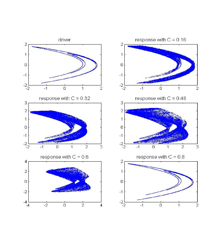
Figure 1: Attractors of driver and response Hénon maps (1) for various couplings.

For each coupling strength a total number of $100000$ were generated by iterative method. The coupling strengths were chosen from $0$ to $0.8$ with the step $0.04.$ The starting point was $[0.7,0,0.7,0].$ First $1000$ data points were thrown away.

The same Hénon-Hénon system has been studied in [25], [22], [17], [27], [13], [18], [23], [9], [31].

The variables of the coupled systems can be arranged into an interaction graph, which is a set of nodes connected by directed edges wherever one variable directly drives another. Based on definitions in [6], in a system of ordinary differential equations, a variable $x$ directly drives $y$ if it appears non-trivially on the right-hand side of the equation for the derivative of $y$. Our two connected Hénon systems represent distinct dynamical subsystems coupled through one-way driving relationship between variables $x_{1}$ and $y_{1}$. See Figure 2. This causal link is what we would like to recover.

Figure 2: Interaction graph for the coupling of two Henon systems.

Estimates of correlation dimension of the combined Hénon-Hénon maps (driver + response), computed for $100000$ numerically generated data lead to values of dimension below $2.44$. The estimate of the dimension of the driving system is about $D_{2}=1.22$ for the same amount of data. $D_{2}$ estimates around the coupling threshold of $0.7$ clearly reveal the onset of synchronization by drop to the value of $1.22$ (the dimension of the driving system) (Figure 3). The same result was indicated by the analysis of the conditional Lyapunov exponent [25].

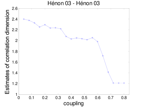
Figure 3: Correlation dimension estimates for two identical Hénon systems (1) connected with different coupling strengths.

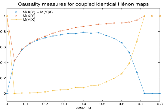
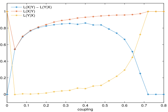
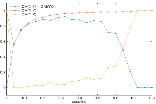
Figure 4: Measures $M$, $L$, and $CM$ computed for uni-directionally coupled identical Hénon systems (1). The measures show that $X$ drives $Y$ until the onset of synchronization around the coupling threshold of $0.7$.

Results of causality detection using reconstructed manifolds

Suppose that we only know $10000$ data-points of variable $x_{1}$ of the driving system and variable $y_{1}$ of the response system from (1) and we would like to know whether there is a causal relationship between the two systems.

One orbit of the attractor has no more than hundred points. In order to use the state-space based methods of search for causality we used delay coordinates with the delay equal to $1$ to reconstruct state portraits of the dynamics in $5-$dimensional state spaces. For the methods $6$ nearest neighbors were taken.

In the following, let us denote the direction from $X$ to $Y$ by $X|Y$ and the direction from $Y$ to $X$ by $Y|X$ . Take, for example the measure $M$. If $X$ drives $Y$, the measure $M(X|Y)$ is expected to be higher than $M(Y|X)$. In figures, $M(X|Y)$ is displayed in red, $M(Y|X)$ in yellow and their difference $\text{$\Delta$}M(X|Y)=M(X|Y)-M(Y|X)$ is shown in blue.

3.2 Hénon $0.3$ $\rightarrow$ Hénon $0.1$

The second example is formed by uni-directionally coupled nonidentical Hénon maps. Variables $x_{1}$, $x_{2}$ correspond to the driver system and $y_{1}$, $y_{2}$ are the variables of the response system:

$$x_{1}(n+1) = 1.4-x_{1}^{2}(n)+0.3x_{2}(n)$$

$$x_{2}(n+1) = x_{1}(n)$$ (2)

$$y_{1}(n+1) = 1.4-\left(Cx_{1}(n)y_{1}(n)+(1-C)y_{1}^{2}(n)\right)+0.1y_{2}(n)$$

$$y_{2}(n+1) = y_{1}(n)$$

The data were generated by iterative method. The coupling strength was chosen from $0$ to $1.4$ with the step $0.04.$ The starting point was $[0.7,0,0.7,0].$ First $1000$ data points were thrown away. The total number of obtained data was $100000.$ This system was investigated in [25], [22], [27]. The interaction graph for this connection is the same as in the previous case (Figure 2).

Figure 5: Coupled non-identical Hénon systems (2). 2-dimensional plots of attractors of driver and response system for various couplings.

Maximum Lyapunov exponent of the response system turns negative near the coupling $0.2$ and rises to positive values around the couplings $0.4-0.5.$ Then it falls again to negative values showing generalized (nonidentical) synchronization [22]. Similar behavior is presented by our estimates of correlation dimension of the $X+Y$ (see Figure 6). The dimension of the attractor of the combined system saturates to the value which remains relatively unchanging for couplings somewhat higher than $1$.

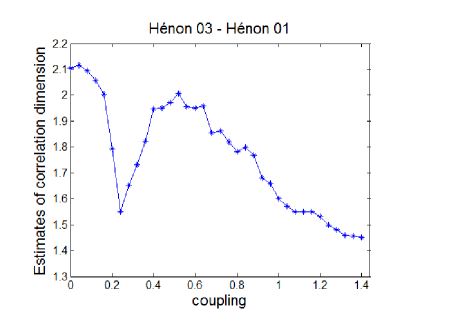
Figure 6: Correlation dimension estimates for two non-identical Hénon systems (2) connected with different coupling strengths.

Results of causality detection using reconstructed manifolds

Suppose that we only know $10000$ data-points of variable $x_{1}$ of the driving system and variable $y_{1}$ of the response system and we would like to know whether there is a causal relationship between the two systems. In order to use the state-space based methods of search for causality we used delay coordinates with the delay equal to $1$ to reconstruct state portraits of the dynamics in $5-$dimensional state spaces. For each method $6$ nearest neighbors were taken.

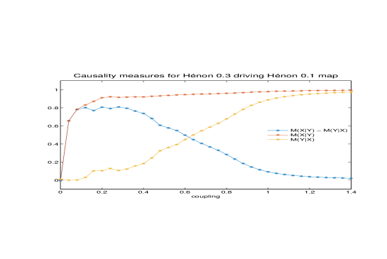
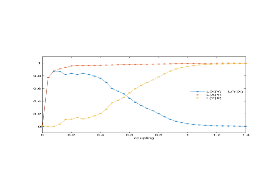
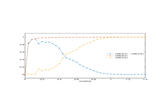
Figure 7: Measures $M$, $L$, and $CM$ computed for uni-directionally coupled non-identical systems (Hénon $0.3$ $\rightarrow$ Hénon $0.1$). The measures show that $X$ drives $Y$ until the onset of synchronization around the coupling threshold of about $1$.

3.3 Hénon $0.1$ $\rightarrow$ Hénon $0.3$

In the next example, the previous two Hénon maps change roles. Now the map with parameter $0.1$ is the driver system and the map with parameter $0.3$ is the response system:

$$x_{1}(n+1) = 1.4-x_{1}^{2}(n)+0.1x_{2}(n)$$

$$x_{2}(n+1) = x_{1}(n)$$ (3)

$$y_{1}(n+1) = 1.4-\left(Cx_{1}(n)y_{1}(n)+(1-C)y_{1}^{2}(n)\right)+0.3y_{2}(n)$$

$$y_{2}(n+1) = y_{1}(n)$$

The data were generated by iterative method. The coupling strength was chosen from $0$ to $1.4$ with the step $0.04.$ The starting point was $[0.7,0,0.7,0].$ First $1000$ data points were thrown out. The total number of obtained data was $100000.$ The same Hénon-Hénon system was used in [22], [17], and [23].

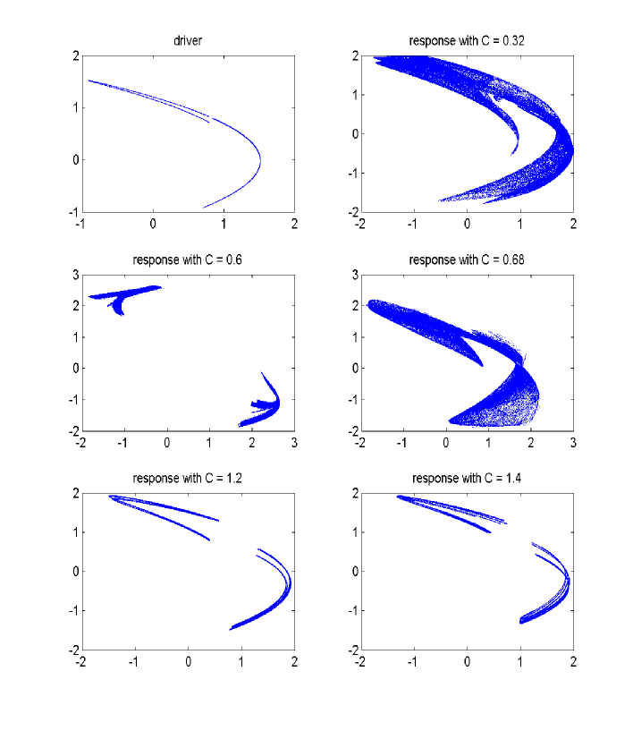
Figure 8: Coupled non-identical Hénon systems (3). 2-dimensional plots of attractors of driver and response system for various couplings.

Also in this case variables of the coupled systems can be arranged into the interaction graph shown in Figure 2. It means that the two connected Hénon systems represent distinct dynamical subsystems coupled through one-way driving relationship between variables $x_{1}$ and $y_{1}$. This causal link is what we would like to recover.

In this example, the correlation dimension of the driving system (estimates about $1.02$) is lower than the dimension of the response system (estimates about $1.22$).

The largest Lyapunov exponent of the response decreases with increasing coupling and becomes negative at $0.38$. After coupling of $0.6$ it rises and touches zero around $0.62$ and then it falls again to negative values, which indicate generalized synchronization of two nonidentical systems [17].

Our estimates of correlation dimension of the $X+Y$ system (Figure 9) show similar declines and risings to finally settle for couplings higher than $1.1$.

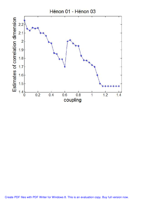
Figure 9: Correlation dimension estimates for two non-identical Hénon systems (3). The individual values correspond to different coupling strengths.

Results of causality detection using reconstructed manifolds

Suppose that we only know $10000$ data-points of variable $x_{1}$ of the driving system and variable $y_{1}$ of the response system and we would like to know whether there is a causal relationship between the two systems. In order to use the state-space based methods of search for causality we used delay coordinates with the delay equal to $1$ to reconstruct state portraits of the dynamics in $5-$dimensional state spaces. For each method $6$ nearest neighbors were taken.

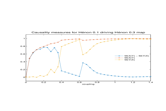
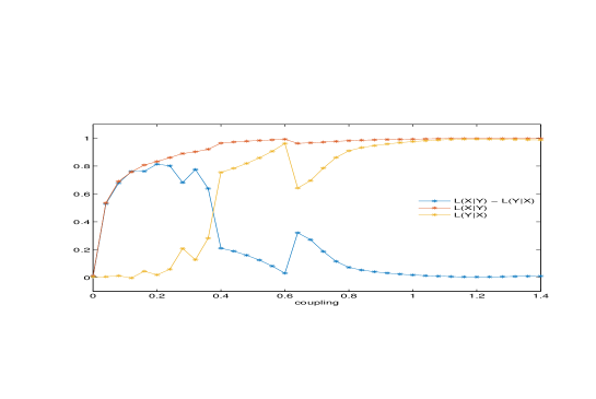
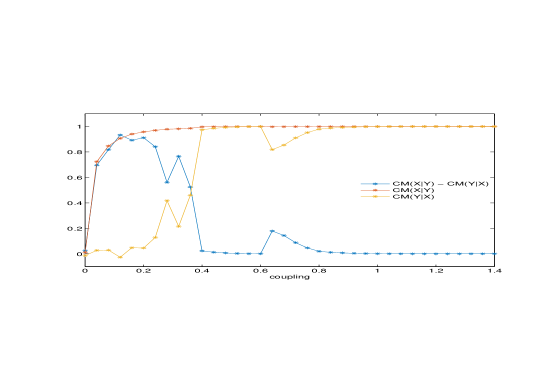
Figure 10: Measures $M$, $L$, and $CM$ computed for uni-directionally coupled non-identical systems (Hénon $0.1$ $\rightarrow$ Hénon $0.3$). The measures show that $X$ drives $Y$ until the onset of synchronization around the coupling threshold of about $1.1$.

3.4 Rössler $\rightarrow$ Lorenz

In this example Rössler system ($x_{1}$, $x_{2}$, $x_{3}$) drives the Lorenz system ($y_{1}$, $y_{2}$, $y_{3}$):

$$\dot{x}_{1} = -6(x_{2}+x_{3})$$

$$\dot{x}_{2} = 6(x_{1}+0.2x_{2})$$

$$\dot{x}_{3} = 6\left(0.2+x_{3}(x_{1}-5.7)\right)$$ (4)

$$\dot{y}_{1} = 10(-y_{1}+y_{2})$$

$$\dot{y}_{2} = 28y_{1}-y_{2}-y_{1}y_{3}+Cx_{2}^{2}$$

$$\dot{y}_{3} = y_{1}y_{2}-\frac{8}{3}y_{3}$$

A total number of $100000$ data were obtained from Matlab solver of ordinary differential equations ode45 which is based on explicit Runge-Kutta formula. The coupling strength was chosen from $0$ to $5$ with the step $0.1$. The starting point was $[0,0,0.4,0.3,0.3,0.3].$ First $1000$ data points were thrown away. The same system was studied in [20], [14], [22], [17], [1] and [18].

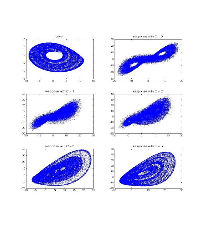
Figure 11: Rössler system driving Lorenz system. 2-dimensional plots of attractors of driver and response system for various couplings.

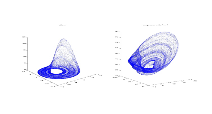
Figure 12: Rössler system driving Lorenz system. 3-dimensional plots of attractors of driver and response system for coupling 5.

The interaction graph in Figure 13 shows that the Rössler and the Lorenz system are coupled through one-way driving relationship between variables $x_{2}$ and $y_{2}$. This causal link is what we would like to recover.

Figure 13: Interaction graph for the coupling of Rössler system and Lorenz system.

For these coupled systems only weak synchronization is considered [22]. Lyapunov exponents show the synchronization takes place between the coupling strengths $2$ and $3$. The same is indicated by our estimates of correlation dimensions (Figure 14).

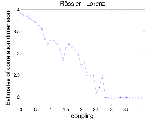
Figure 14: Correlation dimension estimates for Rössler and Lorenz systems connected with different coupling strengths.

Results of causality detection using reconstructed manifolds

Suppose that we know $50000$ data-points of variable $x_{2}$ of the driving Rössler system and variable $y_{2}$ of the responsive Lorenz system and we would like to know whether there is a causal relationship between the two systems. In order to use the state-space based methods of search for causality we made reconstructions of the state portraits. We used time-delayed vectors of $x_{2}$ and $y_{2}$ with time delay equal to $1$ and embedding dimension of $7$. Methods for all three measures used $8$ nearest neighbors.

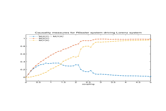
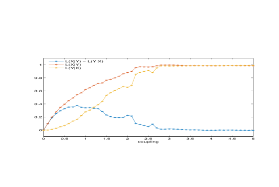
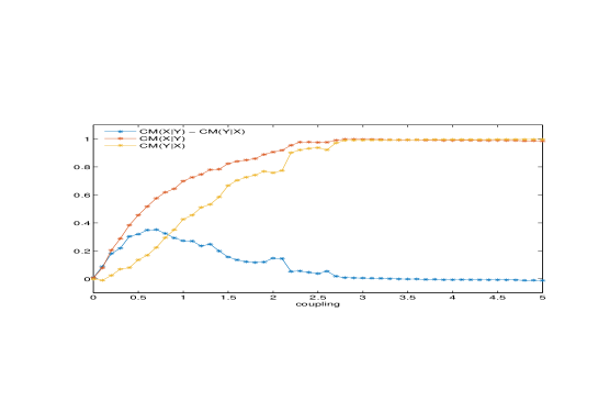
Figure 15: Measures $M$, $L$, and $CM$ computed for uni-directionally coupled Rössler and Lorenz systems. The measures show that $X$ drives $Y$ until the onset of synchronization between the couplings $2$ and $3$.

3.5 Rössler $1.015$ $\rightarrow$ Rössler $0.985$

The fifth data-set comes from coupling of two Rössler systems:

$$\dot{x}_{1} = -\omega_{1}x_{2}-x_{3}$$

$$\dot{x}_{2} = \omega_{1}x_{1}+0.15x_{2}$$

$$\dot{x}_{3} = 0.2+x_{3}(x_{1}-10)$$ (5)

$$\dot{y}_{1} = -\omega_{2}y_{2}-y_{3}+C(x_{1}-y_{1})$$

$$\dot{y}_{2} = \omega_{2}y_{1}+0.15y_{2}$$

$$\dot{y}_{3} = 0.2+y_{3}(y_{1}-10)$$

The parameters $\omega_{1}$, $\omega_{2}$ were set to:

$$\omega_{1}=1.015,\quad\omega_{2}=0.985.$$

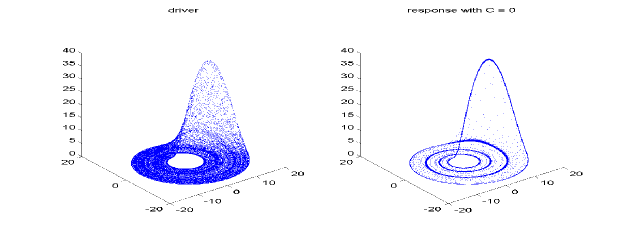
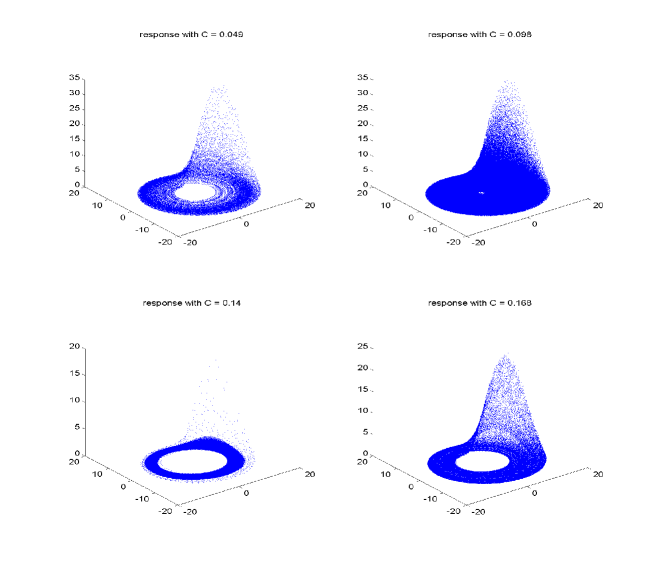
Figure 16: Rössler system ($\omega_{1}=1.015$) driving another Rössler system ($\omega_{2}=0.985$). Attractors of the driver and of response system for various couplings.

The next interaction graph shows that the two Rössler systems are coupled through one-way driving relationship between variables $x_{1}$ and $y_{1}$. This causal link is what we would like to recover.

Figure 17: Interaction graph for the coupling of two Rössler systems.

The data were generated by Matlab solver of ordinary differential equations ode45. The starting point was $[0,0,0.4,0,0,0.4].$ First $1000$ data points were thrown away. The total number of obtained data was $100000$ at an integration step size $0.1.$ This gives about $60$ samples per one average orbit around the attractor. The coupling strength $C$ was chosen from $0$ to $0.2$ with the step $0.01.$ The same system was used in [18], [30], [16].

The plots of the conditional Lyapunov exponents for this Rössler-Rössler system can be found in [18]. They show, similarly as the following graph of $D_{2}$ estimates, that synchronization takes place between couplings $0.11$ and $0.13$.

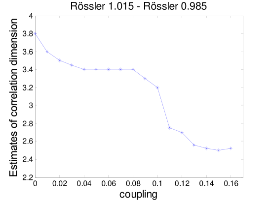
Figure 18: Correlation dimension estimates for two Rössler systems (5) connected with different coupling strengths.

Results of causality detection using reconstructed manifolds

Suppose that we know $50000$ data-points of variable $x_{1}$ of the driving Rössler system and variable $y_{1}$ of the responsive Rössler system and we would like to know whether there is a causal relationship between the two systems. In order to use the state-space based methods of search for causality we made reconstructions of the state portraits. To this end, we used time-delayed vectors of $x_{1}$ and $y_{1}$ with time delay equal to $3$ and embedding dimension of $7$. Methods for all three measures used $8$ nearest neighbors.

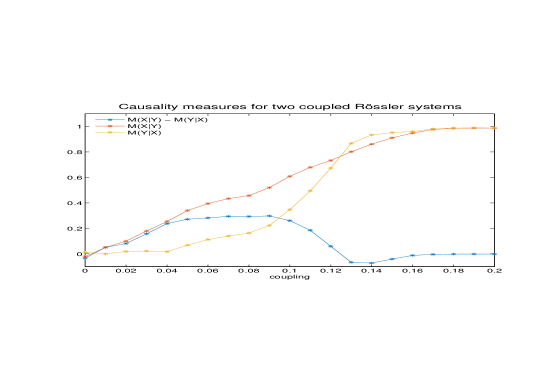
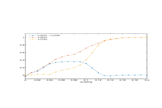
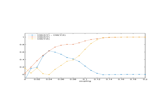
Figure 19: Measures $M$, $L$, and $CM$ computed for two uni-directionally coupled Rössler systems (5). The measures show that $X$ drives $Y$ until the onset of synchronization between couplings $0.11$ and $0.13$.

3.6 Rössler $0.5$ $\rightarrow$ Rössler $2.515$

Another example of coupled Rössler systems:

$$\dot{x}_{1} = -\omega_{1}x_{2}-x_{3}$$

$$\dot{x}_{2} = \omega_{1}x_{1}+a_{1}x_{2}$$

$$\dot{x}_{3} = 0.2+x_{3}(x_{1}-10)$$ (6)

$$\dot{y}_{1} = -\omega_{2}y_{2}-y_{3}+C(x_{1}-y_{1})$$

$$\dot{y}_{2} = \omega_{2}y_{1}+a_{2}y_{2}$$

$$\dot{y}_{3} = 0.2+y_{3}(y_{1}-10)$$

The parameters are set to:

$$\omega_{1}=0.5,\quad\omega_{2}=2.515,\quad a_{1}=0.15,\quad a_{2}=0.72.$$

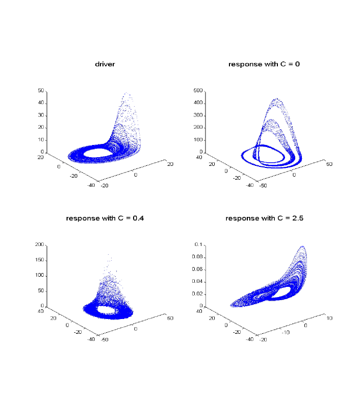
Figure 20: Rössler system ($\omega_{1}=0.5$) driving Rössler system ($\omega_{2}=2.515$). Attractors of the driver and of response system for various couplings.

The frequency ratio of about $1:5$ used in this example reminds cardio-respiratory interactions. The system was used in [18] and in [30] to show that in this case the problem of detecting directionality is much more challenging than detecting directionality in two systems with similar dynamics.

The data were generated by Matlab solver of ordinary differential equations ode45. The coupling strength $C$ was chosen from $0$ to $2.5$ with step size $0.1.$ The starting point was $[0,0,0.4,0,0,0.4].$ First $1000$ data points were thrown away. The total number of obtained data was $100000$ at an integration step size $0.1.$

The variables of the coupled systems may be arranged into the same interaction graph as the previous example. The two connected Rössler systems represent distinct dynamical subsystems coupled through one-way driving relationship between variables $x_{1}$ and $y_{1}$. This causal link is what we tried to uncover.

The plot of the $D_{2}$ estimates shows that synchronization takes place at coupling of about $1$.

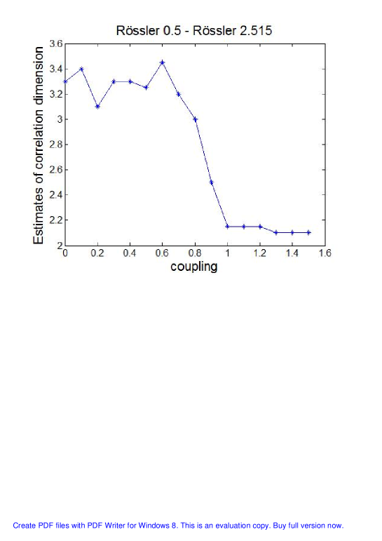
Figure 21: Correlation dimension estimates for two Rössler systems (6) connected with different coupling strengths.

Results of causality detection using reconstructed manifolds

Suppose that we know $50000$ data-points of variable $x_{1}$ of the driving Rössler system and variable $y_{1}$ of the responsive Rössler system and we would like to know whether there is a causal relationship between the two systems.

In order to use the state-space based methods of search for causality we made reconstructions of the state portraits. To this end, we used time-delayed vectors of $x_{1}$ and $y_{1}$ with time delay equal to $1$ and embedding dimension of $7$. Methods for all three measures used $8$ nearest neighbors.

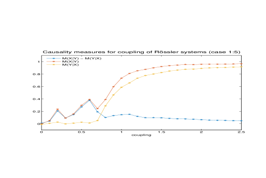
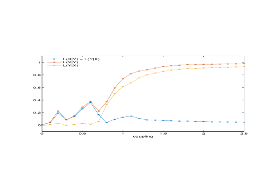
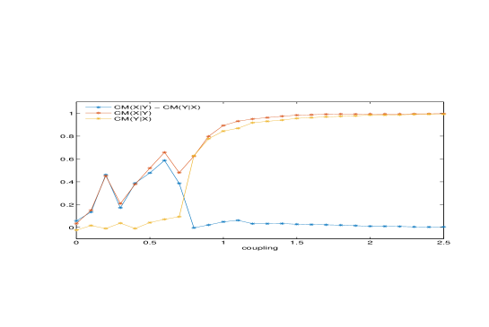
Figure 22: Measures $M$, $L$, and $CM$ computed for two uni-directionally coupled Rössler systems (6). The measures show that $X$ drives $Y$ until the onset of synchronization at coupling of about $1$.

3.7 Rössler $2.515$ $\rightarrow$ Rössler $0.5$

In this example, in reverse to the preceding case, the direction of coupling is from the faster Rössler system to the slower system:

$$\dot{x}_{1} = -\omega_{1}x_{2}-x_{3}$$

$$\dot{x}_{2} = \omega_{1}x_{1}+a_{1}x_{2}$$

$$\dot{x}_{3} = 0.2+x_{3}(x_{1}-10)$$ (7)

$$\dot{y}_{1} = -\omega_{2}y_{2}-y_{3}+C(x_{1}-y_{1})$$

$$\dot{y}_{2} = \omega_{2}y_{1}+a_{2}y_{2}$$

$$\dot{y}_{3} = 0.2+y_{3}(y_{1}-10)$$

The parameters were set to:

$$\omega_{1}=2.515,\quad\omega_{2}=0.5,\quad a_{1}=0.72,\quad a_{2}=0.15.$$

The data were generated by Matlab solver of ordinary differential equations ode45. The values of coupling strength $C$ were chosen from $0$ to $0.5$. The starting point was $[0,0,0.4,0,0,0.4].$ First $2000$ points were thrown away. $100000$ data points obtained at an integration step size $0.1$ were saved. The same system was used in [18] and in [30].

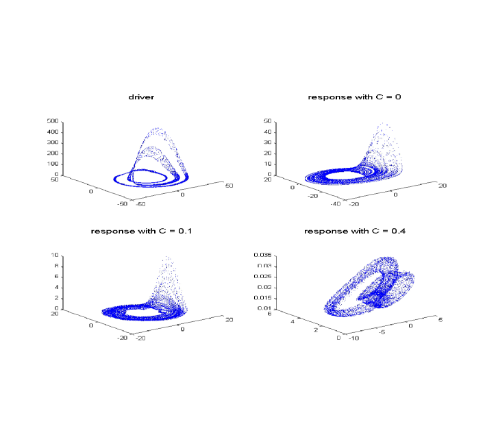
Figure 23: Rössler ($\omega_{1}=0.5$) driving Rössler ($\omega_{2}=2.515$). Attractors of the driver and of response system for various couplings.

The variables of the coupled systems may be once again arranged into the interaction graph shown in Figure 17. It means that the two connected Rössler systems represent distinct dynamical subsystems coupled through one-way driving relationship between variables $x_{1}$ and $y_{1}$. This causal link is what we would like to recover.

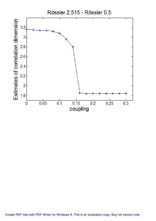
Figure 24: Correlation dimension estimates for two Rössler systems (7) connected with different coupling strengths.

Results of causality detection using reconstructed manifolds

Suppose that we know $50000$ data-points of variable $x_{1}$ of the driving Rössler system and variable $y_{1}$ of the responsive Rössler system and we would like to know whether there is a causal relationship between the two systems.

In order to use the state-space based methods of search for causality we made reconstructions of the state portraits with the same parameters as in the previous case. This means time-delayed vectors of $x_{1}$ and $y_{1}$ with delay equal to $1$ and embedding dimension of $7$. Methods for all three measures used $8$ nearest neighbors.

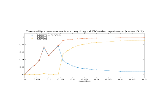
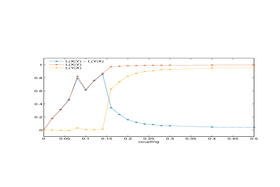
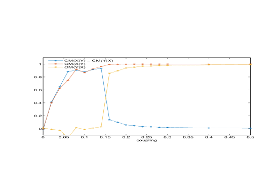
Figure 25: Measures $M$, $L$, and $CM$ computed for two uni-directionally coupled Rössler systems (7). The measures show that $X$ drives $Y$ until the onset of synchronization between couplings $0.15$ and $0.2$.

3.8 Lorenz $28.5$ $\rightarrow$ Lorenz $27.5$

Here the first three lines correspond to the driving Lorenz system and the last three equations characterize the response Lorenz system:

$$\dot{x}_{1} = 10(-x_{1}+x_{2})$$

$$\dot{x}_{2} = 28.5x_{1}-x_{2}-x_{1}x_{3}$$

$$\dot{x}_{3} = x_{1}x_{2}-\frac{8}{3}x_{3}$$ (8)

$$\dot{y}_{1} = 10(-y_{1}+y_{2})+C(x_{1}-y_{1})$$

$$\dot{y}_{2} = 27.5y_{1}-y_{2}-y_{1}y_{3}$$

$$\dot{y}_{3} = y_{1}y_{2}-\frac{8}{3}y_{3}$$

The data were generated by Matlab solver of ordinary differential equations ode45. The coupling strength $C$ was chosen from $0$ to $10.08$ with step $0.42.$ The starting point was $[0.3,0.3,0.3,0.3,0.3,0.3].$ First $20000$ data points was thrown away. The total number of obtained data was $100000$ at an integration step size $0.01.$

The same system was used in [2] to show that for the Lorenz dynamics both the flow waveforms and the events derived from them enable detection of the coupling.

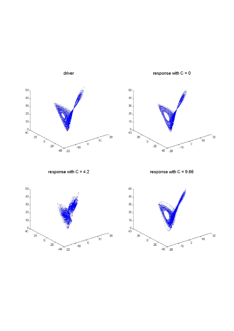
Figure 26: Lorenz $28.5$ driving Lorenz $27.5$. Attractors of driver and response system for various couplings.

The next interaction graph shows that the two Lorenz systems are coupled through driving relationship between variables $x_{1}$ and $y_{1}$. This causal link is what we would like to recover.

Figure 27: Interaction graph for the coupling of two Lorenz systems.

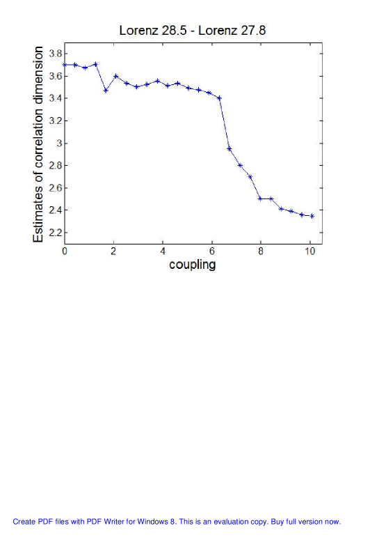
Figure 28: Correlation dimension of connected Lorenz systems (8) for different coupling strengths.

Results of causality detection using reconstructed manifolds

Let us have $50000$ data-points of variable $x_{1}$ and variable $y_{1}.$ In order to use the state-space based methods of search for causality we made reconstructions of the state portraits. To this end, we used time-delayed vectors of $x_{1}$ and $y_{1}$ with time delay equal to $1$ and embedding dimension of $7$. Methods for all three measures used $8$ nearest neighbors.

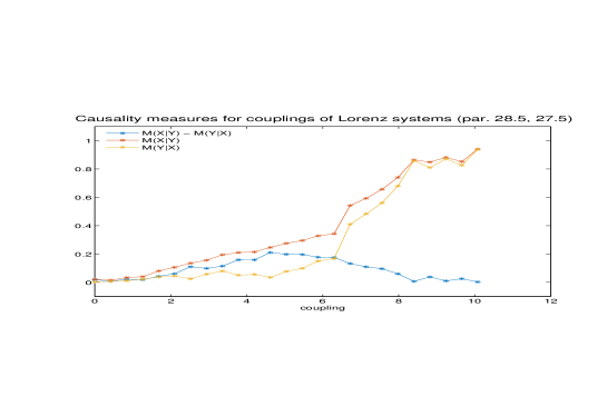
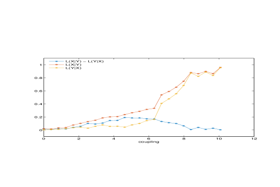
Figure 29: Measures $M$, $L$, and $CM$ computed for two uni-directionally coupled Lorenz systems (8). The measures show that $X$ drives $Y$ until the onset of synchronization between couplings $8$ and $10$.

3.9 Lorenz $39$ $\rightarrow$ Lorenz $35$

The last example is formed by another uni-directionally coupled nonidentical Lorenz systems. Variables $x_{1}$, $x_{2}$, $x_{3}$ correspond to the driver system and $y_{1}$, $y_{2}$, $y_{3}$ are the variables of the response system:

$$\dot{x}_{1} = 10(-x_{1}+x_{2})$$

$$\dot{x}_{2} = 39x_{1}-x_{2}-x_{1}x_{3}$$

$$\dot{x}_{3} = x_{1}x_{2}-\frac{8}{3}x_{3}$$ (9)

$$\dot{y}_{1} = 10(-y_{1}+y_{2})+C(x_{1}-y_{1})$$

$$\dot{y}_{2} = 35y_{1}-y_{2}-y_{1}y_{3}$$

$$\dot{y}_{3} = y_{1}y_{2}-\frac{8}{3}y_{3}$$

The data were generated by Matlab solver of ordinary differential equations ode45. The coupling strength $C$ was chosen from $0$ to $14$ with the step $1.$ The starting point was $[0.3,0.3,0.3,0.3,0.3,0.3].$ First $2000$ data points was thrown away. The total number of obtained data was $100\,000$ at an integration step size $0.01.$ Similar system was used in [5].

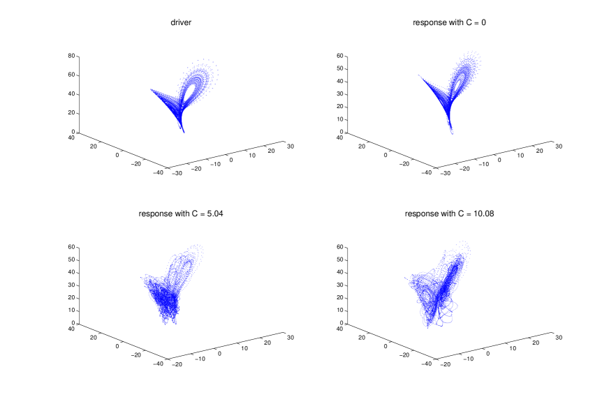
Figure 30: Lorenz $39$ driving Lorenz $35$. Attractors of the driver and of response system for various couplings.

The variables of the coupled systems may be arranged into the same interaction graph as the previous example. The two connected Lorenz systems represent distinct dynamical subsystems coupled through one-way driving relationship between variables $x_{1}$ and $y_{1}$(see Figure 27). This causal link is what we tried to uncover.

Estimates of correlation dimension of the combined Lorenz-Lorenz system (driver + response), computed for $100000$ data saturates to the value which remains relatively unchanging for couplings somewhat higher than $9$:

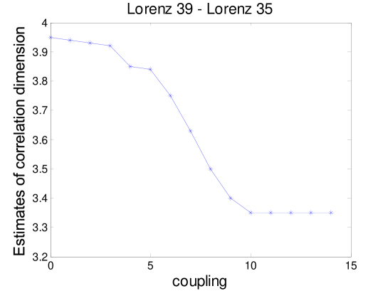
Figure 31: Correlation dimension estimates for two Lorenz systems (9) connected with different coupling strengths.

Results of causality detection using reconstructed manifolds

Suppose that we know $50000$ data-points of variable $x_{1}$ of the driving Lorenz system and variable $y_{1}$ of the responsive Lorenz system and we would like to know whether there is a causal relationship between the two systems.

In order to use the state-space based methods of search for causality we made reconstructions of the state portraits with the same parameters as in the previous case. This means time-delayed vectors of $x_{1}$ and $y_{1}$ with delay equal to $1$ and embedding dimension of $7$. Methods for all three measures used $8$ nearest neighbors.

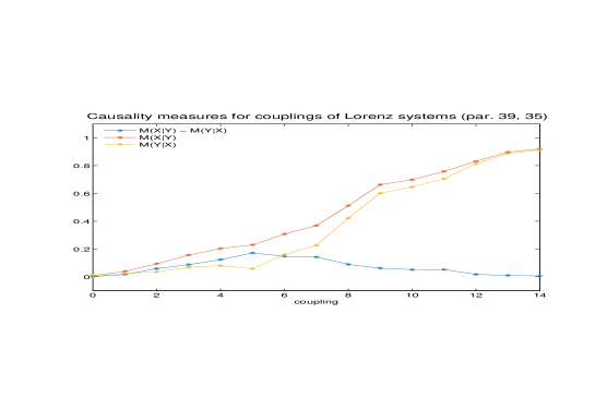
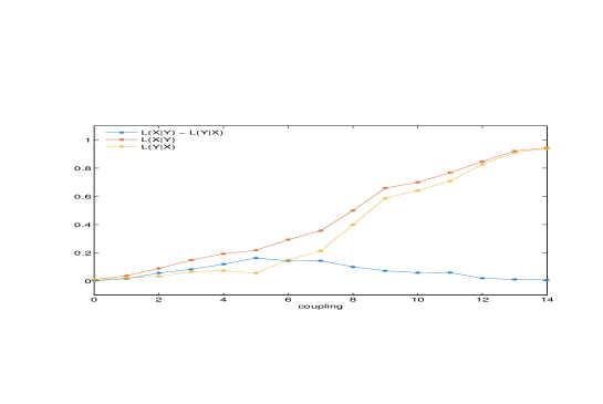
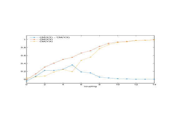
Figure 32: Measures $M$, $L$, and $CM$ computed for two uni-directionally coupled Lorenz systems. The measures show that $X$ drives $Y$ until the onset of synchronization for couplings somewhat higher than $9$.

4 Conclusion

In this study three methods to detect causality in reconstructed state space were tested. The first method is based on measure named $M$ [1], the second one is based on measure $L$ [5], and the third one is a more recent variant of cross-mapping [28].

The methods were compared on test examples of uni-directionally connected chaotic systems of Hénon, Rössler and Lorenz type in relation to the ability to detect unidirectional coupling and synchronization of interconnected dynamical systems.

Results show that each of the three examined methods managed to reveal the presence and the direction of coupling and also to detect the onset of full synchronization. Both the efficiency and the computational complexity of the methods were comparable.

In case of real data, it may happen that the there is a correlation between the systems and that is falsely declared as causality. Then we can take any of the measures and look for performance improvement with increasing number of used data. Lack of convergence means the absence of causality. However, investigating the aspect of convergence of the efficiency is left for further research.

Acknowledgment

This work was supported by the Slovak Grant Agency for Science (Grant no. 2/0043/13).

5 Appendix

5.1 Computation of measures $M,$ $L$ and $CM$

Matlab code prepared by Jozef Jakubík and retrieved in October 2015 from

https://www.mathworks.com/matlabcentral/fileexchange/52964-convergent-cross-mapping/content/SugiLM.m

⬇

1function [ SugiCorr , SugiR , LM , SugiY , SugiX , origY , origX ] = SugiLM( X , Y , tau , E , LMN )

2

3% Calculating Sugihara’s CMM, L and M causality.

4%

5% References:

6% - for Sugihara’s CCM method > Sugihara, George, et al., Detecting Causality in Complex Ecosystems, Science 26 October 2012, Vol. 338, no. 6106, pp. 496-500.

7% - for L method > Chicharro, Daniel, and Ralph G. Andrzejak, Reliable detection of directional couplings using rank statistics, Physical Review E 80.2 (2009): 026217.

8% - for M method > Andrzejak, Ralph G., et al., Bivariate surrogate techniques: necessity, strengths, and caveats, Physical review E 68.6 (2003): 066202.

9%

10% Inputs:

11% X,Y - time series with the same length

12% tau - time step for the reconstruction

13% E - dimension of the reconstruction

14% LMN - number of neighborhoods for L and M methods

15% the number of neighborhoods for Sugihara’s CCM method is E+1

16%

17% Outputs:

18% SugiCorr - correlation between the CCM estimation of original data and original data

19% SugiR - sqrt((sum((originaldata-CCMestimaleddata).^2)/numel(originaldata)))/std(origaldata)

20% LM - results for L and M methods

21% SugiY, SugiX - the CCM estimate of original data

22% origY, origX - original data

23

24switch nargin

25 case 5

26 case 4

27 LMN = E+1;

28 otherwise

29 error(’Bad input’)

30end

31

32L=length(X);

33T=1+(E-1)*tau;

34Xm=zeros((L-T+1),E);

35Ym=zeros((L-T+1),E);

36SugiN=E+1;

37N = L-T+1;

38

39%% RECONTRUCTIONS OF ORIGINAL SYSTEMS

40

41for t=1:(L-T+1)

42 Xm(t,:)=X((T+t-1):-tau:(T+t-1-(E-1)*tau));

43 Ym(t,:)=Y((T+t-1):-tau:(T+t-1-(E-1)*tau));

44end

45%%

46LMj= zeros(2,2,N);

47

48SugiX=zeros(N,1);

49SugiY=zeros(N,1);

50

51parfor j=1:N

52%% neighborhood search

53

54[n1,d1]=knnsearch(Xm,Xm(j,:),’k’,N);

55[n2,d2]=knnsearch(Ym,Ym(j,:),’k’,N);

56

57%% LM

58

59LMn1=n1(n1~=j);

60LMn2=n2(n2~=j);

61LMd1=d1(n1~=j);

62LMd2=d2(n2~=j);

63

64susXY=arrayfun(@(x) find(LMn1(:) == x,1,’first’), LMn2(1:LMN) );

65susYX=arrayfun(@(x) find(LMn2(:) == x,1,’first’), LMn1(1:LMN) );

66

67sum1=sum(LMd1(:))/(N-1);

68sum2=sum(LMd2(:))/(N-1);

69

70LMj(:,:,j) = [(N/2-sum(susXY)/LMN)/(N/2-(LMN+1)/2) , (sum1-sum(LMd1(susXY))/LMN)/(sum1-sum(LMd1(1:LMN))/LMN) ; (N/2-sum(susYX)/LMN)/(N/2-(LMN+1)/2) , (sum2-sum(LMd2(susYX))/LMN)/(sum2-sum(LMd2(1:LMN))/LMN)];

71

72 % (GN-G(Y|X))/(GN-Gk) => L(Y|X)

73 % (GN-G(X|Y))/(GN-Gk) => L(X|Y)

74

75 %(RNY-Rcond(Y|X))/(RNY-RkY) => M(Y|X)

76 %(RNX-Rcond(X|Y))/(RNX-RkX) => M(X|Y)

77end

78

79%% CMM

80

81dat=floor((L-T+1)/2);

82

83parfor ii=(dat+1):(L-T+1)

84 [n1s,d1s]=knnsearch(Xm((ii-dat):(ii-1),:),Xm(ii,:),’k’,SugiN);

85 [n2s,d2s]=knnsearch(Ym((ii-dat):(ii-1),:),Ym(ii,:),’k’,SugiN);

86

87 u1s=exp(-d1s/d1s(1));

88 w1s=u1s/sum(u1s);

89 SugiY(ii)= w1s*Y(n1s+T-1+ii-(dat+1));

90

91 u2s=exp(-d2s/d2s(1));

92 w2s=u2s/sum(u2s);

93 SugiX(ii)= w2s*X(n2s+T-1+ii-(dat+1));

94end

95

96origY=Y(T:end);

97origY=origY((dat+1):(L-T+1));

98SugiY=SugiY((dat+1):(L-T+1));

99origX=X(T:end);

100origX=origX((dat+1):(L-T+1));

101SugiX=SugiX((dat+1):(L-T+1));

102

103%%

104

105SugiCorr1=corrcoef(origY,SugiY);

106SugiCorr(2,1)=SugiCorr1(1,2);

107

108SugiCorr2=corrcoef(origX,SugiX);

109SugiCorr(1,1)=SugiCorr2(1,2);

110

111SugiR(2,1)=sqrt((sum((origY-SugiY).^2)/numel(origY)))/std(origY);

112SugiR(1,1)=sqrt((sum((origX-SugiX).^2)/numel(origX)))/std(origX);

113

114LM = squeeze(mean(LMj,3));

115

116end

References

- [1] Ralph G Andrzejak, Alexander Kraskov, Harald Stögbauer, Florian Mormann, and Thomas Kreuz. Bivariate surrogate techniques: necessity, strengths, and caveats. Physical review E, 68(6):066202, 2003.
- [2] Ralph G Andrzejak and Thomas Kreuz. Characterizing unidirectional couplings between point processes and flows. EPL (Europhysics Letters), 96(5):50012, 2011.
- [3] Jochen Arnhold, Peter Grassberger, Klaus Lehnertz, and Christian Erich Elger. A robust method for detecting interdependences: application to intracranially recorded eeg. Physica D: Nonlinear Phenomena, 134(4):419–430, 1999.
- [4] Lionel Barnett, Adam B Barrett, and Anil K Seth. Granger causality and transfer entropy are equivalent for gaussian variables. Physical review letters, 103(23):238701, 2009.
- [5] Daniel Chicharro and Ralph G. Andrzejak. Reliable detection of directional couplings using rank statistics. Phys. Rev. E, 80:026217, Aug 2009.
- [6] Bree Cummins, Tomáš Gedeon, and Kelly Spendlove. On the efficacy of state space reconstruction methods in determining causality. SIAM Journal on Applied Dynamical Systems, 14(1):335–381, 2015.
- [7] Clive WJ Granger. Investigating causal relations by econometric models and cross-spectral methods. Econometrica: Journal of the Econometric Society, pages 424–438, 1969.
- [8] P. Grassberger and I. Procaccia. Measuring the strangeness of strange attractors. Physica D, 9(1-2):189–208, 1983.
- [9] S Janjarasjitt and KA Loparo. An approach for characterizing coupling in dynamical systems. Physica D: Nonlinear Phenomena, 237(19):2482–2486, 2008.
- [10] M. B. Kennel, R. Brown, and H. D. I. Abarbanel. Determining embedding dimension for phase-space reconstruction using a geometricial construction. Phys Rev A, 45(69):3403–3411, 1992.
- [11] Anna Krakovská and Hana Budáčová. Interdependence measure based on correlation dimension. In Proceedings of the 9th International Conference on Measurement, pages 31–34. ISBN 978-80-969-672-5-4, 2013.
- [12] Anna Krakovská, Kristína Mezeiová, and Hana Budáčová. Use of false nearest neighbours for selecting variables and embedding parameters for state space reconstruction. article id 932750. Journal of Complex Systems, 2015, 2015.
- [13] Thomas Kreuz, Florian Mormann, Ralph G Andrzejak, Alexander Kraskov, Klaus Lehnertz, and Peter Grassberger. Measuring synchronization in coupled model systems: A comparison of different approaches. Physica D: Nonlinear Phenomena, 225(1):29–42, 2007.
- [14] Michel Le Van Quyen, Jacques Martinerie, Claude Adam, and Francisco J Varela. Nonlinear analyses of interictal eeg map the brain interdependences in human focal epilepsy. Physica D: Nonlinear Phenomena, 127(3):250–266, 1999.
- [15] C. Lutz. Granger causality test - matlab function. 2009.
- [16] Milan Paluš. Cross-scale interactions and information transfer. Entropy, 16(10):5263–5289, 2014.
- [17] Milan Paluš, Vladimír Komárek, Zbyněk Hrnčíř, and Katalin Štěrbová. Synchronization as adjustment of information rates: detection from bivariate time series. Physical Review E, 63(4):046211, 2001.
- [18] Milan Paluš and Martin Vejmelka. Directionality of coupling from bivariate time series: How to avoid false causalities and missed connections. Phys. Rev. E, 75(5):056211, 2007.
- [19] Louis M Pecora and Thomas L Carroll. Synchronization in chaotic systems. Physical review letters, 64(8):821, 1990.
- [20] K Pyragas. Weak and strong synchronization of chaos. Physical Review E, 54(5):R4508, 1996.
- [21] R. Quian Quiroga, A. Kraskov, T. Kreuz, and P. Grassberger. Performance of different synchronization measures in real data: A case study on electroencephalographic signals. Phys. Rev. E, 65(4):041903, 2002.
- [22] R. Quian Quiroga, J. Arnhold, and P. Grassberger. Learning driver-response relationships from synchronization patterns. Phys. Rev. E, 61:5142–5148, May 2000.
- [23] M Carmen Romano, Marco Thiel, Jürgen Kurths, and Celso Grebogi. Estimation of the direction of the coupling by conditional probabilities of recurrence. Physical Review E, 76(3):036211, 2007.
- [24] Nikolai F Rulkov, Mikhail M Sushchik, Lev S Tsimring, and Henry DI Abarbanel. Generalized synchronization of chaos in directionally coupled chaotic systems. Physical Review E, 51(2):980, 1995.
- [25] Steven J Schiff, Paul So, Taeun Chang, Robert E Burke, and Tim Sauer. Detecting dynamical interdependence and generalized synchrony through mutual prediction in a neural ensemble. Physical Review E, 54(6):6708, 1996.
- [26] Thomas Schreiber. Measuring information transfer. Physical review letters, 85(2):461, 2000.
- [27] CJ Stam and BW Van Dijk. Synchronization likelihood: an unbiased measure of generalized synchronization in multivariate data sets. Physica D: Nonlinear Phenomena, 163(3):236–251, 2002.
- [28] George Sugihara, Robert May, Hao Ye, Chih-hao Hsieh, Ethan Deyle, Michael Fogarty, and Stephan Munch. Detecting causality in complex ecosystems. science, 338(6106):496–500, 2012.
- [29] F. Takens. Detecting strange attractors in turbulence. In D. A. Rand and L. S. Young, editors, Dynamical Systems and Turbulence, pages 366–381. Springer-Verlag, Berlin, 1981.
- [30] Martin Vejmelka and Milan Paluš. Inferring the directionality of coupling with conditional mutual information. Physical Review E, 77(2):026214, 2008.
- [31] Ioannis Vlachos and Dimitris Kugiumtzis. Nonuniform state-space reconstruction and coupling detection. Physical Review E, 82(1):016207, 2010.