Quantum optimal control of photoelectron spectra and angular distributions

Abstract

Photoelectron spectra and photoelectron angular distributions obtained in photoionization reveal important information on e.g. charge transfer or hole coherence in the parent ion. Here we show that optimal control of the underlying quantum dynamics can be used to enhance desired features in the photoelectron spectra and angular distributions. To this end, we combine Krotov’s method for optimal control theory with the time-dependent configuration interaction singles formalism and a splitting approach to calculate photoelectron spectra and angular distributions. The optimization target can account for specific desired properties in the photoelectron angular distribution alone, in the photoelectron spectrum, or in both. We demonstrate the method for hydrogen and then apply it to argon under strong XUV radiation, maximizing the difference of emission into the upper and lower hemispheres, in order to realize directed electron emission in the XUV regime.

I Introduction

Photoelectron spectroscopy is a powerful tool for studying photoionization in atoms, molecules and solids Hüfner (2003); Meyer et al. (2010); Fabre et al. (1981); Becker and Shirley (1996); Wu et al. (2011); Blaga et al. (2009). With the advent of new light sources, photoelectron spectroscopy using intense, short pulses has become available, revealing important information about electron dynamics and time-dependent phenomena Krausz and Ivanov (2009); Wabnitz et al. (2002); Corkum and Krausz (2007); Kanter et al. (2011). In particular, it allows for characterizing the light-matter interaction of increasingly complex systems Hüfner (2003); Wu et al. (2011); Fabre et al. (1981). Photoelectron spectra (PES) and photoelectron angular distributions (PAD) contain not only fingerprints of the interaction of the electrons with the electromagnetic fields, but also of their interaction and their correlations with each other Schwarz (1980). PAD in particular can be used to uncover electron interactions and correlations Duinker (1982); Reid (2003).

Tailoring the pulsed electric field in its amplitude, phase or polarization allows to control the electron dynamics, with corresponding signatures in the photoelectron spectrum Meier and Engel (1994); Shen and Engel (2002); Wollenhaupt et al. (2005); Gräfe et al. (2005); Braun et al. (2014). While it is natural to ask how the electron dynamics is reflected in the experimental observables—PES and PAD Meier and Engel (1994); Shen and Engel (2002); Wollenhaupt et al. (2005); Gräfe et al. (2005); Braun et al. (2014), it may also be interesting to see whether one can control or manipulate directly these observables by tailoring the excitation pulse. Moreover, one may be interested in certain features such as directed electron emission without analyzing all the details of the time evolution. This is particularly true for complex systems where it may not be easy to trace the full dynamics all the way to the spectrum. The question that we ask here is how to find an external field that steers the dynamics such that the resulting photoelectron distribution fulfills certain prescribed properties. Importantly, the final state of the dynamics does not need to be known. The desired features may be reflected in the angle-integrated PES, the energy-integrated PAD, or both.

To answer this question, we employ optimal control theory (OCT), using Krotov’s monotonically convergent method Reich et al. (2012) and adapting it to the specific task of realizing photoelectron distributions with prescribed features. The photoelectron distributions are calculated within the time-dependent configuration interaction singles scheme (TDCIS) Greenman et al. (2010), employing the splitting method for extracting the spectral components from the outgoing wavepacket Karamatskou et al. (2014, 2015). While OCT has been utilized to study the quantum control of electron dynamics before, in the framework of TDCIS Klamroth (2006) as well as the multi-configurational time-dependent Hartree-Fock (MCTDHF) method Mundt and Tannor (2009) or time-dependent density functional theory (TDDFT) Castro et al. (2012); Hellgren et al. (2013), the PES and PAD have not been tackled as control targets before. In fact, most previous studies did not even account for the presence of the ionization continuum. A proper representation of the ionization continuum becomes unavoidable McCurdy and Rescigno (1997); Martín (1999); Rescigno and McCurdy (2000); Bachau et al. (2001); McCurdy and Martín (2004), however, when investigating the interaction with XUV light where a single photon is sufficient to ionize Greenman et al. (2014), and it is indispensable for the full description of photoionization experiments.

To demonstrate the versatility of our approach, we apply it to two different control problems: (i) We prescribe the full three-dimensional photoelectron distribution and search for a field that produces, at least approximately, a given angle-integrated PES and energy-integrated PAD. Such a detailed control objective is rather demanding and corresponds to a difficult control problem. (ii) We seek to maximize the relative number of photoelectrons emitted into the upper as opposed to the lower hemisphere, assuming that the polarization axis of the light pulse runs through the poles of the two hemispheres. This implies a condition on the PAD alone, leaving complete freedom to the energy dependence. The corresponding control objective leaves considerable freedom to the optimization algorithm and the control problem becomes much simpler. Maximizing the relative number of photoelectrons emitted into the upper as opposed to the lower hemisphere corresponds to a maximization of the PAD’s asymmetry. Asymmetric photoelectron distributions arising in strong-field ionization were studied previously for near-infrared few-cycle pulses where the effect was attributed to the carrier envelope phase Rathje et al. (2013); Shvetsov-Shilovski et al. (2014). Here, we pose the question whether it is possible to achieve asymmetry in the PAD for multiphoton ionization in the XUV regime and we seek to determine the shaped pulse that steers the electrons into one hemisphere. To ensure experimental feasibility of the optimized pulses, we introduce spectral as well as amplitude constraints. We test our control toolbox for hydrogen and argon atoms, corresponding to a single channel and three active channels, respectively. These comparatively simple examples allow for a complete discussion of our optimization approach, while keeping the numerical effort at an acceptable level.

The remainder of this paper is organized as follows. Section II briefly reviews the methodology for describing the electron dynamics, with Sec. II.1 devoted to the TDCIS method, and Sec. II.2 presenting the wave function splitting approach. Optimal control theory for photoelectron distributions is developed in Sec. III. Specifically, we introduce the optimization functionals to prescribe a certain PES plus PAD and to generate directed photoelectron emission in Sec. III.1. The corresponding optimization algorithms are presented in Sec. III.2, emphasizing the combination of OCT with the wave function splitting method. For the additional functionality of restricting the spectral bandwidth of the field in the optimization, the reader is referred to Appendix A. Our numerical results are presented in Sec. IV to VI, demonstrating, for hydrogen, the prescription of the PES and PAD in Sec. IV and the minimization of photoelectron emission into the lower hemisphere in Sec. V. Maximization of the relative number of photoelectrons emitted into the upper hemisphere is discussed for both hydrogen and argon in Sec. VI. Finally, Sec. VII concludes.

II Theory

In the following, we briefly review, following Refs. Greenman et al. (2010); Karamatskou et al. (2014), the theoretical framework for describing the electron dynamics and the interaction with strong electric fields.

II.1 First principles calculation of the $N$-particle wave function: TDCIS

Our method for calculating the outgoing electron wave packet is based on the time-dependent configuration interaction singles (TDCIS) scheme Greenman et al. (2010); Pabst et al. (Rev 1425, 2014). The time-dependent Schrödinger equation of the full $N$-electron system,

$$i\frac{\partial}{\partial t}|\Psi(t)\rangle = \hat{H}(t)|\Psi(t)\rangle\,,$$ (1)

is solved numerically using the Lanczos-Arnoldi propagator Leforestier et al. (1991); Kosloff (1994). To this end, the $N$-electron wave function is expanded in the one-particle–one-hole basis:

$$|\Psi(t)\rangle = \alpha_{0}(t)|\Phi_{0}\rangle+\sum_{i,a}\alpha_{i}^{a}(t)|\Phi_{i}^{a}\rangle,$$ (2)

where the index $i$ denotes an initially occupied orbital, $a$ stands for a virtual orbital to which the particle can be excited and $|\Phi_{0}\rangle$ symbolizes the Hartree-Fock ground state. The full time dependent Hamiltonian has the form

$$\hat{H}(t) = \hat{H}_{0}+\hat{H}_{1}+\hat{\mathbf{p}}\cdot{\mathbf{A}}(t),$$ (3)

where $\hat{H}_{0}=\hat{T}+\hat{V}_{\rm nuc}+\hat{V}_{\rm MF}-E_{\rm HF}$ contains the kinetic energy $\hat{T}$, the nuclear potential $\hat{V}_{\rm nuc}$, the potential at the mean-field level $\hat{V}_{\rm MF}$ and the Hartree-Fock energy $E_{\rm HF}$. $\hat{H}_{1}=\frac{1}{|r_{12}|}-\hat{V}_{\rm MF}$ describes the Coulomb interactions beyond the mean-field level, and $\hat{\mathbf{p}}\cdot\mathbf{A}(t)$ is the light-matter interaction within the velocity form in the dipole approximation, assuming linear polarization.

The TDCIS approach is a multi-channel method, i.e., all ionization channels that lead to a single excitation of the system are included in the calculation. Since only states with total spin $S=0$ are considered, only spin singlets occur and we denote the occupied orbitals by $|\phi_{i}\rangle$. As introduced in Ref. Rohringer et al. (2006), for each ionization channel all single excitations from the occupied orbital $|\phi_{i}\rangle$ may be collected in one “channel wave function”:

$$|\varphi_{i}(t)\rangle = \sum_{a}\alpha_{i}^{a}(t)|\phi_{a}\rangle\,$$ (4)

where the summation runs over all virtual orbitals, labeled with $a$, which is a multi-index Greenman et al. (2010). These channel wave functions allow to calculate all quantities in a channel-resolved manner Karamatskou et al. (2014, 2015). In the actual implementation, the orbitals in Eq. (4) are expressed as a product of radial and angular parts Karamatskou et al. (2014); Greenman et al. (2010),

$$\phi_{a}(\mathbf{r}) = \frac{u^{n_{a}}_{\ell_{a}}(r)}{r}\,Y^{\ell_{a}}_{m_{a}}(\vartheta_{r},\varphi_{r})\,,$$ (5)

where $Y^{l}_{m}$ denote the spherical harmonics and $u^{n}_{l}(r)$ is the radial part of the wave function which is represented on a pseudo-spectral spatial grid Greenman et al. (2010).

II.2 The wave function splitting method

The PES and PAD are calculated using the splitting method Tong et al. (2006) which was implemented within the TDCIS scheme Karamatskou et al. (2014, 2015). Briefly, in this propagation approach the wave function is split into an inner and an outer part using a smooth radial splitting function,

$$\hat{S} = \left[1+e^{-(\hat{r}-r_{c})/\Delta}\right]^{-1}\,,$$ (6)

where the parameter $\Delta$ controls how steep the slope of the function is and $r_{c}$ is the splitting radius. The channel wave functions (4) are used to calculate the spectral components in a channel-resolved manner by projecting the outer part onto Volkov states, $|\mathbf{p}\,\!^{V}\rangle=(2\pi)^{-3/2}e^{i\mathbf{p}\cdot\mathbf{r}}$. To this end, each channel wavefunction is split into an inner and an outer part at every splitting time $t_{j}$,

$$|\varphi_{i}(t_{j})\rangle = |\varphi_{i,\rm in}(t_{j})\rangle+|\varphi_{i,\rm out}(t_{j})\rangle$$ (7a)

where

$$|\varphi_{i,\rm in}(t_{j})\rangle = (1-\hat{S})|\varphi_{i}(t_{j})\rangle$$ (7b)

and

$$|\varphi_{i,\rm out}(t_{j})\rangle = \hat{S}|\varphi_{i}(t_{j})\rangle$$ (7c)

At each splitting time, the inner part, $|\varphi_{i,\rm in}(t_{j})\rangle$, is represented in the CIS basis and further propagated with the full Hamiltonian (3), whereas the outer part is stored and propagated analytically to large times with the Volkov Hamiltonian,

$$\hat{H}_{V}(\tau) = \frac{1}{2}\left[\hat{\mathbf{p}}+\mathbf{A}(\tau)\right]^{2}\,.$$ (8)

In this way, the outer part of the wave function can be analyzed separately in order to obtain information on the photoelectron. Furthermore, since the outgoing part of the wave function is absorbed efficiently at the splitting times, large box sizes are avoided in the inner region.

The spectral coefficient $\varphi_{i}(\mathbf{p},T;t_{j})$ for a given channel $i$, originating from splitting time $t_{j}$ and evaluated at the final time $t=T$ is obtained as a function of the momentum vector $\mathbf{p}$ Karamatskou et al. (2014),

$$\varphi_{i,\rm out}(\mathbf{p},T;t_{j})=\int d^{3}p^{\prime}\langle\mathbf{p}\,^{V}|\hat{U}_{V}(T,t_{j})|\mathbf{p}\,^{\prime}\,\!{}^{V}\rangle\langle\mathbf{p}\,^{\prime}\,\!{}^{V}|\varphi_{i,\rm out}(t_{j})\rangle=\dfrac{2}{\pi}e^{-i\vartheta_{V}(\mathbf{p})}\sum_{a}(-i)^{l_{a}}\beta_{i}^{a}(t_{j})Y^{l_{a}}_{m_{a}}(\Omega_{\mathbf{p}})\int_{0}^{\infty}dr\,ru^{n_{a}}_{l_{a}}(r)j_{l_{a}}(pr)\,,$$ (9)

where $\vartheta_{V}(\mathbf{p})$ denotes the Volkov phase, given by

$$\vartheta_{V}(\mathbf{p}) = \frac{1}{2}\int_{t_{j}}^{T}d\tau\,\left[\mathbf{p}+\mathbf{A}(\tau)\right]^{2}\,,$$ (10)

the sum runs over the virtual orbitals, $\beta^{a}_{i}(t_{j})$ is the overlap of the outer part with the virtual orbital,

$$\beta^{a}_{i}(t_{j}) = \langle\phi_{a}|\varphi_{i,\rm out}(t_{j})\rangle\,,$$ (11)

and $j_{l}(x)$ is the $l$th Bessel function. $\hat{U}_{V}(t_{2},t_{1})=\exp\left(-i\int_{t_{1}}^{t_{2}}\hat{H}_{V}(\tau)d\tau\right)$ is the evolution operator associated with the Volkov Hamiltonian (8) and $T$ is a sufficiently long time so that all parts of the wave function that are of interest have reached the outer region and are included in the PES. The contributions from all splitting times must be added up coherently to form the total spectral coefficient for the channel $i$,

$$\tilde{\varphi}_{i,\rm out}(\mathbf{p},T) = \sum_{t_{j}}\varphi_{i,\rm out}(\mathbf{p},T;t_{j}).$$ (12)

Finally, incoherent summation over all possible ionization channels yields the total spectrum Karamatskou et al. (2014),

$$\frac{d^{2}\sigma(\mathbf{p})}{dp\,d\Omega}=\big{|}\tilde{\varphi}_{\rm out}(\mathbf{p},T)\big{|}^{2}=\sum_{i}\big{|}\tilde{\varphi}_{i,\rm out}(\mathbf{p},T)\big{|}^{2}\,.$$ (13)

The energy-integrated PAD is given by integrating over energy or, equivalently, momentum,

$$\dfrac{d\sigma}{d\Omega} = \int^{\infty}_{0}\dfrac{d^{2}\sigma(\mathbf{p})}{dpd\Omega}\,p^{2}dp\,.$$ (14a)

Analogously, the angle-integrated PES is obtained upon integration over the solid angle,

$$\dfrac{d\sigma}{dE} = p\int^{2\pi}_{0}\int^{\pi}_{0}\dfrac{d^{2}\sigma(\mathbf{p})}{dpd\Omega}\,\sin\theta d\theta d\phi$$ (14b)

with $p=\sqrt{2E}$. The optimizations considered below are based on these measurable quantities.

III Optimal control theory

III.1 Optimization problem

Our goal is to find a vector potential, or control, $\mathbf{A}(t)$, that steers the system from the ground state $|\Psi(t=0)\rangle=|\Phi_{0}\rangle$, defined in Eq. (2), to an unknown final state $|\Psi(T)\rangle$ whose PES and/or PAD display certain desired features. Such an optimization target is expressed mathematically as a final time functional $J_{T}[\tilde{\varphi}_{\rm out},\tilde{\varphi}_{\rm out}^{\dagger}]$ Reich et al. (2012). We consider two different final time optimization functionals in the following.

As a first example, we seek to prescribe the angle-integrated PES and energy-integrated PAD together. The corresponding final time cost functional is defined as

$$J^{(1)}_{T}[\tilde{\varphi}_{\rm out}(T),\tilde{\varphi}^{\dagger}_{\rm out}(T)] = \lambda_{1}\int\left(\tilde{\sigma}(\mathbf{p},T))-\tilde{\sigma}_{0}(\mathbf{p})\right)^{2}\,d^{3}p\,,\quad\quad$$ (15)

where $\tilde{\sigma}(\mathbf{p},T)=d^{2}\sigma(\mathbf{p})/dp\,d\Omega$ denotes the actual photoelectron distribution, cf. Eq. (13), $\tilde{\sigma}_{0}(\mathbf{p})$ stands for the target distribution, and $\lambda_{1}$ is a weight that stresses the importance of $J^{(1)}_{T}[\tilde{\varphi}_{\rm out},\tilde{\varphi}^{\dagger}_{\rm out}]$ compared to additional terms in the total optimization functional. The goal is thus to minimize the squared Euclidean distance between the actual and the desired photoelectron distributions.

Alternatively, we would like to control the difference in the number of electrons emitted into the lower and upper hemispheres. This can be expressed via the following final-time functional

$$J^{(2)}_{T}[\tilde{\varphi}_{\rm out}(T),\tilde{\varphi}^{\dagger}_{\rm out}(T)]=$$ (16)

$$\quad\quad\quad\quad\lambda_{2}^{(-)}\int^{\pi}_{\pi/2}\sin\theta\,d\theta\int_{0}^{+\infty}\big{|}\tilde{\varphi}_{\rm out}(\mathbf{p},T)\big{|}^{2}p^{2}\,dp$$

$$\quad\quad\quad\quad+\lambda_{2}^{(+)}\int^{\pi/2}_{0}\sin\theta\,d\theta\int_{0}^{+\infty}\big{|}\tilde{\varphi}_{\rm out}(\mathbf{p},T)\big{|}^{2}p^{2}\,dp$$

$$\quad\quad\quad\quad+\lambda_{2}^{tot}\int^{\pi}_{0}\sin\theta\,d\theta\int_{0}^{+\infty}\big{|}\tilde{\varphi}_{\rm out}(\mathbf{p},T)\big{|}^{2}p^{2}\,dp\,,$$

where the first and second term correspond to the probability of the photoelectron being emitted into the lower and upper hemisphere, whereas the third term is the total ionization probability. $\lambda_{2}^{(-)}$, $\lambda_{2}^{(+)}$ and $\lambda_{2}^{tot}$ are weights. The factor of $2\pi$ resulting from integration over the azimuthal angle has been absorbed into the weights. Directed emission can be achieved in several ways—one can suppress the emission of the photoelectron into the lower hemisphere, without imposing any specific constraint on the number of electrons emitted into the upper hemisphere. This is achieved by choosing $\lambda^{(+)}_{2}=\lambda^{tot}_{2}=0$ and $\lambda^{(-)}_{2}>0$. Alternatively, one can maximize the difference in the number of electrons emitted into the upper and lower hemispheres. To this end, the relative weights need to be chosen such that $\lambda^{(-)}_{2}>0$ and $\lambda^{(+)}_{2}<0$. If $\lambda^{tot}_{2}=0$, the optimization seeks to increase the absolute difference in the number of electrons emitted into the upper and lower hemisphere. Close to an optimum, this may result in a strong increase in the overall ionization probability, accompanied by a very small increase in the difference, since only the complete functional is required to converge monotonically, and not each of its parts. This undesired behavior can be avoided by maximizing the relative instead of the absolute difference of electrons emitted into the upper and lower hemispheres. It requires $\lambda^{tot}_{2}>0$, i.e., minimization of the total ionization probability in addition to maximizing the difference. Note that $\lambda_{2}^{tot}$ could also be absorbed into the weights for the hemispheres,

$$J^{(2)}_{T}[\tilde{\varphi}_{\rm out}(T),\tilde{\varphi}^{\dagger}_{\rm out}(T)]=$$ (17)

$$\quad\quad\quad\quad+\lambda^{(-)}_{eff}\int^{\pi}_{\pi/2}\sin\theta\,d\theta\int_{0}^{+\infty}\big{|}\tilde{\varphi}_{\rm out}(\mathbf{p},T)\big{|}^{2}p^{2}\,dp$$

$$\quad\quad\quad\quad+\lambda^{(+)}_{eff}\int^{\pi/2}_{0}\sin\theta\,d\theta\int_{0}^{+\infty}\big{|}\tilde{\varphi}_{\rm out}(\mathbf{p},T)\big{|}^{2}p^{2}\,dp\,,$$

where $\lambda^{(+)}_{eff}=-|\lambda_{2}^{(+)}|+|\lambda^{tot}_{2}|$ and $\lambda^{(-)}_{eff}=|\lambda_{2}^{(-)}|+|\lambda^{tot}_{2}|$ are effective weights. Since $\lambda^{(+)}_{eff}<0$ and $\lambda^{(-)}_{eff}>0$ in order to maximize (minimize) emission into the upper (lower) hemisphere, the weights need to fulfill the condition $|\lambda^{(+)}_{2}|>|\lambda^{tot}_{2}|$.

The complete functional to be minimized,

$$J = J_{T}[\tilde{\varphi}_{\rm out}(T),\tilde{\varphi}^{\dagger}_{\rm out}(T)]+C[\mathbf{A}]\,,$$ (18)

also includes constraints $C[\mathbf{A}]$ to ensure that the control remains finite or has a limited spectral bandwidth. The constraints may be written for the electric field $\mathbf{E}(t)$ associated with the vector potential $\mathbf{A}(t)$, even though the minimization problem is expressed in terms of $\mathbf{A}(t)$ and the dynamics is generated by $\hat{H}[\mathbf{A}]$, cf. Eq. (3). The relation between the vector potential $\mathbf{A}(t)$ and the electric field $\mathbf{E}(t)$ is given by

$$\mathbf{A}(t) = -\int_{t_{0}}^{t}\mathbf{E}(\tau)\,d\tau\,.$$ (19)

with $\mathbf{A}(t_{o})=\mathbf{0}$. Without loss of generality, we can write

$$C[\mathbf{A}] = C_{a}[\mathbf{A}]+C_{\omega}[\mathbf{A}]+C_{e}[\mathbf{A}],\$$ (20)

where the independent terms in the rhs. of Eq. (20) are defined below.

The first property that the optimized electric field must fulfill is that its integral over time vanishes, i.e.,

$$\int_{t_{0}}^{T}\mathbf{E}(t)\,dt = 0\,,$$ (21)

which implies, according to Eq. (19), $\mathbf{A}(T)=\mathbf{A}(t_{0})=0$. Therefore, we choose initial guess fields with $\mathbf{A}(T)=\mathbf{A}(t_{0})=0$ and utilize

$$C_{a}[\mathbf{A}] = \lambda_{a}\int s^{-1}(t)\left(\mathbf{A}(t)-\mathbf{A}_{\rm ref}(t)\right)^{2}\,dt$$ (22)

with $s(T)=0$ to ensure that Eq. (21) is fulfilled. In Eq. (22), $\mathbf{A}_{\rm ref}(t)$ and $s(t)$ refer to a reference vector potential and a shape function, respectively, and $\lambda_{a}\geq 0$ is a weight that stresses the importance of $C_{a}[\mathbf{A}]$ compared to all other terms in the complete functional, Eq. (18). The shape function, $s(t)$, can be used to guarantee that the control is smoothly switched on and off at the initial and final times.

A second important property of the optimized field is a limited spectral bandwidth. Typically, optimization without spectral constraints leads to pulses with unnecessarily broad spectra which would be very hard or impossible to produce experimentally. To restrict the bandwidth of the electric field, $\mathbf{E}(t)$, we construct a constraint $C_{\omega}[\mathbf{A}]$ in frequency domain,

$$C_{\omega}[\mathbf{A}] = \lambda_{\omega}\int\tilde{\gamma}(\omega)\big{|}\tilde{\mathbf{E}}(\omega)\big{|}^{2}\,d\omega$$ (23)

$$= \lambda_{\omega}\int\tilde{\gamma}(\omega)\omega^{2}\big{|}\tilde{\mathbf{A}}(\omega)\big{|}^{2}\,d\omega\,,$$

with $\tilde{\mathbf{E}}(\omega)$ being the Fourier transform of the field,

$$\tilde{\mathbf{E}}(\omega) = \int\mathbf{E}(t)\,e^{-i\omega t}\,dt\,.$$ (24)

Constraints of the form of Eq. (23) were previously discussed in Refs. Palao et al. (2013); Reich et al. (2014): The kernel $\tilde{\gamma}(w)$ plays a role similarly to the inverse shape function $s^{-1}(t)$ in Eq. (22), that is, it takes large values at all undesired frequencies. Additionally, we assume that the symmetry requirement $\tilde{\gamma}(\omega)=\tilde{\gamma}(-\omega)$ is fulfilled, see Appendix A for details.

Finally, in view of experimental feasibility, we would also like to limit the amplitude of the electric field to reasonable values. To this end, we construct a constraint that penalizes changes in the first time derivative of $\mathbf{A}(t)$. In fact, since $\mathbf{E}(t)=-\dot{\mathbf{A}}(t)$, large values in the derivative of the vector potential translate into large amplitudes of the corresponding electric field $\mathbf{E}(t)$. To avoid this, we adopt here a modified regularization condition Hohenester et al. (2007) for $\mathbf{A}(t)$, defining

$$C_{e}[\mathbf{A}] = \lambda_{e}\int s^{-1}(t)|{\mathbf{E}}(t)|^{2}\,dt$$ (25)

$$= \lambda_{e}\int s^{-1}(t)|\dot{\mathbf{A}}(t)|^{2}\,dt\,.$$

$C_{e}[\mathbf{A}]$ plays the role of a penalty functional Hohenester et al. (2007), ensuring the regularity of $\mathbf{A}(t)$, and, as a consequence, penalizing large values on the electric field amplitude $\mathbf{E}(t)$. The choice of the same $s^{-1}(t)$ in both Eq. (22) and Eq. (25) will simplify the optimization algorithm as shown below.

III.2 Krotov’s method combined with wave function splitting

Krotov’s method for quantum optimal control provides a recipe to construct monotonically convergent optimization algorithms, depending on the target functional and additional constraints, the type of equation of motion, and the power of the control in the light-matter interaction Reich et al. (2012). The optimization algorithm consists of a set of coupled equations for the update of the control, the forward propagation of the state and the backward propagation of the so-called co-state. This set of equations needs to be solved iteratively. The final-time target functional (or, more precisely, its functional derivative with respect to the propagated state, evaluated at the final time, which reflects the extremum condition on the optimization functional Palao and Kosloff (2003)) determines the “initial” condition, at final time, for the backward propagation of the co-state Reich et al. (2012). Additional constraints which depend on the control such as those in Eq. (20) show up in the update equation for the control Reich et al. (2012, 2014). The challenge when combining Krotov’s method with the wave function splitting approach is due to the fact that splitting in the forward propagation of the state implies “glueing” in the backward propagation of the co-state. Here, we present an extension of the optimization algorithm obtained with Krotov’s method that takes the splitting procedure into account.

Evaluating the prescription given in Refs. Reich et al. (2012, 2014), we find for the update equation, with $k$ labeling the iteration step,

$$\mathbf{A}^{(k+1)}(t) = \mathbf{A}^{(k)}(t)+I^{(k+1)}(t)$$

$$-\frac{\tilde{\lambda}_{\omega}}{\lambda_{a}}s(t)\mathbf{A}^{(k+1)}\star h(t)+\frac{\lambda_{e}}{\lambda_{a}}\ddot{\mathbf{A}}^{(k+1)}(t)\,,$$

with $$\tilde{\lambda}_{\omega}=\sqrt{2\pi}\lambda_{\omega} \mathbf{A}^{(k+1)}\star h(t) \mathbf{A}^{(k+1)} h(t)$$. denotes the convolution of and ,

$$\mathbf{A}^{(k+1)}\star h(t) = \int\mathbf{A}^{(k+1)}(\tau)\,h(t-\tau)\,d\tau\,$$ (26b)

with $$h(t) \tilde{h}(\omega)=\omega^{2}\tilde{\gamma}(\omega)$$ the inverse Fourier transform of . The second term in Eq. (26) is given by

$$I^{(k+1)}(t) = \frac{s(t)}{\lambda_{a}}\mathfrak{Im}\left\{\left\langle\chi^{(k)}(t)\left|\frac{\partial\hat{H}}{\partial\mathbf{A}}\right|\Psi^{(k+1)}(t)\right\rangle\right\}$$ (26c)

$$= \frac{s(t)}{\lambda_{a}}\mathfrak{Im}\left\{\langle\chi^{(k)}(t)|\hat{\mathbf{p}}|\Psi^{(k+1)}(t)\rangle\right\}\,,$$

where $|\Psi^{(k+1)}(t)\rangle$ and $|\chi^{(k)}(t)\rangle$ denote the forward propagated state and backward propagated co-state at iterations $k+1$ and $k$, respectively. The derivation of Eqs. (26) is detailed in Appendix A. In order to evaluate Eqs. (26), the co-state obtained at the previous iteration, $|\chi^{(k)}(t)\rangle$, using the old control, $\mathbf{A}^{(k)}(t)$, must be known. Its equation of motion is found to be Reich et al. (2012)

$$i\frac{\partial}{\partial t}|\chi(t)\rangle = \hat{H}(t)|\chi(t)\rangle\,.$$ (27a)

Just as $$|Psi(t)\rangle T$$ is decomposed into channels wavefunctions, cf. Eq. (4), so is the co-state. The “initial” condition at the final time is written separately for each channel,

$$|\tilde{\chi}_{i,\rm out}(T)\rangle = -\frac{\partial J_{T}[\tilde{\varphi}_{i,\rm out}(T),\tilde{\varphi}^{\dagger}_{i,\rm out}(T)]}{\partial\langle\tilde{\varphi}_{i,\rm out}(T)|}\,.$$ (27b)

Evaluation of Eq. (27b) requires knowledge of the outer part of each channel wavefunction, $|\tilde{\varphi}_{i,\rm out}(T)\rangle$, which is obtained by forward propagation of the initial state, including the splitting procedure. In what follows, $\hat{U}(t^{\prime},\tau;\mathbf{A}(t))$ denotes the evolution operator that propagates a given state from time $t=\tau$ to $t=t^{\prime}$ under the control $\mathbf{A}(t)$. We distinguish the time evolution operators for the inner part, $\hat{U}_{F}(t^{\prime},\tau;\mathbf{A}(t))$, generated by the full Hamiltonian, Eq. (3), and for the outer part, $\hat{U}_{V}(t^{\prime},\tau;\mathbf{A}(t))$, generated by the Volkov Hamiltonian, Eq. (8). For every channel, the total wavefunction is given by

$$|\varphi_{i}^{(k+1)}(t)\rangle = |\varphi_{i,\rm in}^{(k+1)}(t)\rangle+|\tilde{\varphi}_{i,\rm out}^{(k+1)}(t)\rangle\,,$$ (28)

which is valid for arbitrary times $t\geq t_{1}$ with $t_{1}$ the first splitting time. The second term in Eq. (28) reads

$$|\tilde{\varphi}^{(k+1)}_{i,\rm out}(t)\rangle = \sum^{\lfloor t/t_{1}\rfloor}_{j=1}|\varphi_{i,\rm out}^{(k+1)}(t;t_{j})\rangle$$ (29)

$$= \sum^{\lfloor t/t_{1}\rfloor}_{j=1}\hat{U}_{V}(t,t_{j};\mathbf{A}^{(k+1)})\,|\varphi_{i,\rm out}^{(k+1)}(t_{j})\rangle\quad$$

with $\lfloor x\rfloor=\rm max\{m\in{Z},m\leq x\}$. Equation (29) accounts for the fact that for $t\geq t_{2}$, all outer parts $|\varphi^{(k+1)}_{i,\rm out}(t;t_{j})\rangle$ that originate at splitting times $t_{j}\leq t$ must be summed up coherently. Propagation of all $|\varphi^{(k+1)}_{i,\rm out}(t;t_{j})\rangle$ and continued splitting of $|\varphi^{(k+1)}_{i,\rm in}(t)\rangle$ eventually yields the state at final time, $|\varphi^{(k+1)}_{i}(T)\rangle$. Its outer part is given by

$$|\tilde{\varphi}^{(k+1)}_{i,\rm out}(T)\rangle = \sum^{N}_{j=1}\,|\varphi^{(k+1)}_{i,\rm out}(T;t_{j})\rangle\,,$$ (30)

where $N$ denotes the number of splitting times utilized during propagation, and the last splitting time $t_{N}$ is chosen such that $t_{N}\leq T$. The best compromise between size of the spatial grid, time step and duration between two consecutive splitting times is discussed in Ref. Karamatskou et al. (2014).

Equation (27b) can now be evaluated: Since our final time functionals all involve the product $\tilde{\varphi}_{\rm out}(\mathbf{p},T)\cdot\tilde{\varphi}_{\rm out}^{*}(\mathbf{p},T)=\sigma(\mathbf{p},T)$, Eq. (27b) can be written, at the $k$th iteration of the optimization, as

$$\tilde{\chi}^{(k)}_{i,\rm out}(\mathbf{p},T)=\mu(\mathbf{p})\,\tilde{\varphi}^{(k)}_{i,\rm out}(\mathbf{p},T)\,,$$ (31a)

where $$\mu(\mathbf{p})$$ is a function that depends on the target functional under consideration. It becomes

$$\mu_{1}^{(k)}(\mathbf{p})=-2\lambda_{1}\left(\tilde{\sigma}^{(k)}(\mathbf{p},T)-\tilde{\sigma}_{0}(\mathbf{p})\right)$$ (31b)

for $$J_{T}^{(1)}$$ given in Eq. (15) and

$$\mu_{2}(\mathbf{p})=\lambda_{2}^{-}\,\leavevmode\hbox{\small 1\kern-3.3pt\normalsize 1}_{\vartheta_{-}}(\theta)+\lambda_{2}^{+}\,\leavevmode\hbox{\small 1\kern-3.3pt\normalsize 1}_{\vartheta_{+}}(\theta)$$ (31c)

for $$J_{T}^{(2)}$$ given in Eq. (16).

The intervals $\vartheta_{-}=[\pi/2,\pi]$ and $\vartheta_{+}=[0,\pi/2]$ denote the lower and upper hemispheres, respectively, and $\leavevmode\hbox{\small 1\kern-3.3pt\normalsize 1}_{\vartheta_{\pm}}(\theta)$ is the characteristic function on a given interval,

$$\leavevmode\hbox{\small 1\kern-3.3pt\normalsize 1}_{\vartheta_{\pm}}(\theta)=\begin{cases}1&\text{if}\ \theta\in\vartheta_{\pm}\\ 0&\text{if}\ \theta\notin\vartheta_{\pm}\end{cases}$$

with $\theta\in[0,\pi]$ the polar angle with respect to the polarization axis. According to Eqs. (1) and (27a), or, more precisely, since we do not consider intermediate-time constraints that depend on the state of the system Reich et al. (2012), $|\Psi(t)\rangle$ and its co-state $|\chi(t)\rangle$ obey the same equation of motion. For that reason, it is convenient to define inner and outer parts of $|\chi(t)\rangle$, analogously to the forward propagated state,

$$|\chi_{i}^{(k)}(t)\rangle = |\chi_{i,\rm in}^{(k)}(t)\rangle+|\tilde{\chi}_{i,\rm out}^{(k)}(t)\rangle\,.$$ (32a)

with

$$|\tilde{\chi}^{(k)}_{i,\rm out}(T)\rangle=\sum^{N}_{j=1}\,|\chi^{(k)}_{i,\rm out}(T;t_{j})\rangle\,.$$ (32b)

Eq. (32b) implies that also $|\tilde{\chi}^{(k)}_{i,\rm out}(T)\rangle$ is obtained by coherently summing up the contributions from all splitting times.

Conversely, the outer part of the co-state originating at the splitting time $t_{j}$ and evaluated at the same time is given by

$$\chi^{(k)}_{i,\rm out}(\mathbf{p},t_{j};t_{j})=\mu(\mathbf{p})\varphi^{(k)}_{i,\rm out}(\mathbf{p},t_{j};t_{j})\,.$$ (33)

The next step is to construct the total co-state at an arbitrary time $t$, $|\chi^{(k)}_{i}(t)\rangle$, required in Eq. (26), from all $|\chi^{(k)}_{i,\rm out}(t_{j};t_{j})\rangle$ using Eq. (33). This is achieved by backward propagation and “glueing” inner and outer parts, as opposite to “splitting” during the forward propagation. However, when reconstructing the co-state by backward propagation, care should be taken to not to perform the “glue” procedure twice or more, at a given splitting time. The backward propagation of the co-state is explicitly explained in what follows: Since at the final time $T$, the total co-state is given by a coherent superposition of all outer parts originating at the splitting times $t_{j}$, cf. Eq. (32b), it suffices to store all $|\varphi^{(k)}_{i,\rm out}(t_{j};t_{j})\rangle$ and apply Eq. (33) to evaluate $|{\chi}^{(k)}_{i,\rm out}(t_{j};t_{j})\rangle$. We recall that $|{\chi}^{(k)}_{i,\rm out}(t_{j};t_{j})\rangle$, respectively $|{\phi}^{(k)}_{i,\rm out}(t_{j};t_{j})\rangle$, denote the outer part born exclusively at $t=t_{j}$ and evaluated at the same splitting time. Once all outer parts of the co-state are evaluated at every splitting time using Eq. (33), $|\chi^{(k)}_{i}(t)\rangle$ is obtained for all times $t$ by backward propagation and “’glueing”, with the additional care of not “glueing” twice or more. In detail, $|{\chi}^{(k)}_{i,\rm out}(t_{N};t_{N})\rangle$ is propagated backwards from $t_{N}$ to $t_{N-1}$ using the full CIS Hamiltonian, $\hat{H}$, cf. Eq. (3). The resulting wave function at $t=t_{N-1}$ is $|\chi^{(k)}_{i,\rm in}(t_{N-1})\rangle$. The outer part born exclusively at the splitting time $t=t_{N-1}$ is obtained using Eq. (33), and the “composite” wave function $|{\chi}^{(k)}_{i}(t_{N-1})\rangle$ is obtained by “glueing” $|\chi^{(k)}_{i,\rm in}(t_{N-1})\rangle$ and $|\chi^{(k)}_{i,\rm out}(t_{N-1};t_{N-1})\rangle$,

$$|{\chi}^{(k)}_{i}(t_{N-1})\rangle=|\chi^{(k)}_{i,\rm in}(t_{N-1})\rangle+|\chi^{(k)}_{i,\rm out}(t_{N-1};t_{N-1})\rangle\,.$$

The procedure is now repeated: the composite co-state $|{\chi}^{(k)}_{i}(t_{N-1})\rangle$ is propagated backwards from $t=t_{N-1}$ to $t=t_{N-2}$ using the full CIS Hamiltonian, resulting in $|\chi^{(k)}_{i,\rm in}(t_{N-2})\rangle$, and “glueing” yields the composite wave function at $t=t_{N-2}$,

$$|{\chi}^{(k)}_{i}(t_{N-2})\rangle=|\chi^{(k)}_{i,\rm in}(t_{N-2})\rangle+|\chi^{(k)}_{i,\rm out}(t_{N-2};t_{N-2})\rangle\,,$$

with $|\chi^{(k)}_{i,\rm out}(t_{N-2},t_{N-2})\rangle$ given by Eq. (33); and so on and so forth for all splitting times $t_{j}$, until $t=t_{0}$, where $t_{0}$ refers to the initial time. During the backward propagation, as described above, the resulting co-state is stored in CIS basis. It gives by construction, at an arbitrary time $t$, the first term in Eq. (32a). The second term in Eq. (32a) involving the outer parts “born” at the splitting times $t=t_{j}$ and evaluated at $t>t_{j}$ is merely given by forward propagating analytically all $|\chi_{i,\rm out}(t_{j};t_{j})\rangle$ using the Volkov Hamiltonian, and summing them up coherently according to Eq. (29). This allows to calculate the “total” co-state wavefunction at an arbitrary time $t$, analogously to $|\varphi_{i}(t)\rangle$. Finally, Eqs. (32a) and (28) allow for evaluating Krotov’s update equation for the control, Eq. (26), where the iteration label just indicates whether the guess, $\mathbf{A}^{(0)}(t)$, the old, $\mathbf{A}^{(k)}(t)$, or the new control, $\mathbf{A}^{(k+1)}(t)$, enter the propagation of $|\chi_{i}(t)\rangle$ and $|\varphi_{i}(t)\rangle$, respectively. A difficulty in solving the update equation for the control, is given by the fact that Eq. (26) is implicit in $\mathbf{A}^{(k+1)}(t)$. Strategies to overcome this obstacle depend on the additional constraints.

III.3 Additional constraints

Implicitness of Eq. (26) in $\mathbf{A}^{(k+1)}(t)$ for $\lambda_{\omega}=\lambda_{e}=0$ can easily be circumvented by a zeroth-order solution, employing two shifted time grids, one for the states, which are evaluated at $n\Delta t$,  and another one for the control, which is evaluated at $(n+1/2)\Delta t$ Palao and Kosloff (2003). However, for $\lambda_{\omega}\neq 0$, Eq. (26) corresponds to a second order Fredholm equation with inhomogeneity $I^{(k+1)}(t)$ Reich et al. (2014). Numerical solution is possible using, for example, the method of degenerate kernels Reich et al. (2014). To this end, the inhomogeneity $I^{(k+1)}(t)$, which depends on $|\varphi^{(k+1)}(t)\rangle$ and thus on $\mathbf{A}^{(k+1)}(t)$, is first approximated to zeroth order by solving Eq. (26) with $\lambda_{\omega}=0$  that is, without frequency constraints; and the resulting approximation $I_{0}^{(k+1)}(t)$ is then used to solve the Fredholm equation. While an iterative procedure to improve the approximation of $I^{(k+1)}(t)$ is conceivable, the zeroth order approximation was found to be sufficient in Refs. Palao et al. (2013); Reich et al. (2014). Here, we adopt a slightly different procedure, in the sense that the Fredholm equation is not solved in time domain but in frequency domain. This allows us to treat the cases $\lambda_{\omega}\neq 0$ and $\lambda_{e}\neq 0$ on the same footing. It is made possible by assuming that $s(t)$ in Eqs. (22) and (25) rises and falls off very quickly at the beginning and end of the optimization time interval. This judicious choice of $s(t)$ together with the fact that the Fourier transform of a convolution of two functions in time domain, as encountered in Eq. (26), is the product of the functions in frequency domain, allows to approximate

$$\left|\int s(t){\Gamma}^{(k+1)}(t)\,e^{-i\omega t}dt-S_{0}\int{\Gamma}^{(k+1)}(t)\,e^{-i\omega t}dt\right| \leq \epsilon\,,$$

where $\epsilon$ is a small, positive number and $\Gamma^{(k+1)}(t)$ is defined as

$${\Gamma}^{(k+1)}(t)=\mathbf{A}^{(k+1)}\star h(t)\,.$$ (35)

A possible choice for $s(t)$ to fulfill the condition (LABEL:epsilon) is

$$s(t) = e^{-\beta((t-t_{c})/2\sigma)^{2n}}\,,$$ (36)

where $\sigma$ refers to the duration of the pulse centered at $t=t_{c}$. If Eq. (LABEL:epsilon) is satisfied, we can easily take the Fourier transform of both sides of Eq. (26) to get

$$\tilde{\mathbf{A}}^{(k+1)}(\omega) = \dfrac{\tilde{\mathbf{A}}^{(k)}(\omega)+\tilde{I}^{(k+1)}(\omega)}{1+\dfrac{\tilde{\lambda}_{\omega}}{\lambda_{a}}\omega^{2}\tilde{\gamma}(\omega)+\dfrac{\lambda_{e}}{\lambda_{a}}\omega^{2}}$$ (37a)

with $$\mathbf{A}^{(k+1)}(t)=\int\tilde{\mathbf{A}}^{(k+1)}(\omega)\,e^{+i\omega t}\,d\omega/\sqrt{2\pi} s(t) \tilde{I}^{(k+1)}(\omega)$$. Note that Eq. (37a) becomes exact if is constant. Approximating by its zeroth order solution analogously to Ref. Reich et al. (2014), Eq. (37a) can be expressed as

$$\tilde{\mathbf{A}}^{(k+1)}(\omega) = \tilde{G}(\omega)\,{\tilde{\mathbf{A}}}_{0}^{(k+1)}(\omega)\,,$$ (37b)

where $$\tilde{\mathbf{A}}_{0}^{(k+1)}(\omega) \lambda_{\omega}=\lambda_{e}=0$$ is the zeroth order solution of the updated control, found by solving Eq. (26) with ,

$$\tilde{\mathbf{A}}_{0}^{(k+1)}(\omega) = \tilde{\mathbf{A}}^{(k)}(\omega)+\tilde{I}^{(k+1)}_{0}(\omega)\,,$$ (37c)

and $$\tilde{G}(\omega)$$ is a transfer function given by

$$\tilde{G}(\omega)=\left(1+\dfrac{\lambda_{\omega}}{\lambda_{a}}\omega^{2}\tilde{\gamma}(\omega)+\dfrac{\lambda_{e}}{\lambda_{a}}\omega^{2}\right)^{-1}\,.$$ (37d)

III.4 Summary of the algorithm

The complete implementation of the optimization within the time-splitting framework of the TDCIS method is summarized as follows:

1. Choose an initial guess for the vector potential, $\mathbf{A}^{(k=0)}(t)$.

2. Forward propagation of the state:

   1. Propagate $|\Psi^{(k=0)}(t=0)\rangle$, cf. Eq. (2), from $t=0$ until the first splitting time, $t=t_{1}$, in the CIS basis. We label the projection of the propagated state onto the channel wavefunctions defined in Eq. (4) by $i=1,2,\dots$, while $i=0$ is reserved for the projection onto the Hartree-Fock ground state.

   2. At $t=t_{1}$, apply the splitting function defined in Eq. (6) to obtain $|\varphi^{(k)}_{i,\rm in}(t_{1})\rangle$ and $|\varphi^{(k)}_{i,\rm out}(t_{1};t_{1})\rangle$. Store the outer part in the CIS representation, before transforming $|\varphi^{(k)}_{i,\rm out}(t_{1};t_{1})\rangle$ to the Volkov representation.

   3. Propagate $|\varphi^{(k)}_{i,\rm in}(t_{1})\rangle$ using $\hat{H}$ and $|\varphi^{(k)}_{i,\rm out}(t_{1};t_{1})\rangle$ using $\hat{H}_{V}$ from $t=t_{1}$ to the next splitting time, $t=t_{2}$.

   4. At $t=t_{2}$, apply the splitting function to $|\varphi^{(k)}_{i,\rm in}(t_{2})\rangle$, again store the resulting outer part in CIS representation, and transform $|\varphi^{(k)}_{i,\rm out}(t_{2};t_{2})\rangle$ to the Volkov representation.

   5. Propagate $|\varphi^{(k)}_{i,\rm in}(t_{2})\rangle$ using $\hat{H}$ and $|\tilde{\varphi}^{(k)}_{i,\rm out}(t_{2})\rangle=|\varphi^{(k)}_{i,\rm out}(t_{2};t_{1})\rangle+|\varphi^{(k)}_{i,\rm out}(t_{2};t_{2})\rangle$ using $\hat{H}_{V}$ from $t=t_{2}$ to the next splitting time $t=t_{3}$.

   6. Repeat steps (2d) and (2e) for all remaining splitting times $t_{j}$ up to $t_{N}$.

   7. Propagate for each channel wave function, $|\tilde{\varphi}^{(k)}_{i,\rm out}(t_{N})\rangle=\sum_{t_{j}=t_{1}}^{t_{N}}|\varphi^{(k)}_{i,\rm out}(t_{N};t_{j})\rangle$ from the last splitting time, $t=t_{N}$, to the final time, $t=T$, to obtain $|\tilde{\varphi}^{(k)}_{i,\rm out}(T)\rangle$ and evaluate the target functional $J_{T}$.

   8. Calculate $\chi^{(k)}_{i,\rm out}(\mathbf{p},T)$ according to Eq. (31a).

3. Backward propagation of the co-state:

   1. Calculate $\mu(\mathbf{p},T)$ according to Eq. (31b) or (31c).

   2. Calculate $|\chi^{(k)}_{i,\rm out}(t_{N};t_{N})\rangle$ from Eq. (33) and propagate it backwards using $\hat{H}$ from $t=t_{N}$ to the previous splitting time $t_{N-1}$. The resulting state is $|\chi^{(k)}_{i,\rm in}(t_{N-1})\rangle$.

   3. At $t=t_{N-1}$, calculate $|\chi^{(k)}_{i,\rm out}(t_{N-1};t_{N-1})\rangle$ from Eq. (33) and ’glue’ to obtain $|{\chi}^{(k)}_{i}(t_{N-1})\rangle=|\chi^{(k)}_{k,\rm in}(t_{N-1})\rangle+|\chi^{(k)}_{i,\rm out}(t_{N-1};t_{N-1})\rangle$. This procedure is performed in the CIS basis for each channel wave function.

   4. Propagate $|{\chi}^{(k)}_{i}(t_{N-1})\rangle$ from $t=t_{N-1}$ to $t_{N-2}$ using $\hat{H}$ to obtain $|\chi^{(k)}_{i,\rm in}(t_{N-2})\rangle$.

   5. Repeat steps (3c) and (3d) for all remaining splitting times and propagate backward up to $t=0$. During the backward propagation, the resulting wavefunction is stored in the CIS basis. As previously detailed, this procedure allows for performing the “glueing” procedure only once at every splitting time. It gives gives rises to the first term in Eq. (32a). The second term involving the evaluation of the outer part (coherent summation) at any arbitrary time $t$ is obtained upon application Eq. (29) to each of the individual contribution $|\chi_{i,\rm out}(t_{j};t_{j})\rangle$ for all splitting times.

4. Forward propagation and update of control:

   1. Determine the zeroth order approximation of the new control at times $(n+1/2)\Delta t$, $\mathbf{A}_{0}^{(k+1)}(n+1/2\Delta t)$, from Eq. (26), using the states at times $n\Delta t$, i.e., the co-state obtained in step 3, $|\chi^{(k)}_{i}(n\Delta t)\rangle$ and $|\varphi^{(k+1)}_{i}(n\Delta t)\rangle$ obtained with the control $\mathbf{A}^{(k+1)}((n-1/2)\Delta t)$.

   2. If $\lambda_{\omega}\neq 0$ or $\lambda_{e}\neq 0$, solve Eq. (37b) to obtain $\tilde{\mathbf{A}}^{(k+1)}(\omega)$, using the approximated $\mathbf{A}^{(k+1)}_{0}(t)$, and Fourier transform $\tilde{\mathbf{A}}^{(k+1)}(\omega)$ to time domain.

5. Increase $k$ by one and repeat steps 3 and 4 until convergence of $J_{T}$ is reached.

At this point, we would like to stress that the parameters chosen for the momentum grid require particular attention for the optimization algorithm to work. This is due to the transformation from the CIS representation to the Volkov basis (CIS–to–$p$ transformation) at each splitting time, as discussed in Section II.2. During the backward propagation, correspondingly, the inverse transformation is required, i.e., the $p$–to–CIS transformation. The CIS–to–$p$ transformation of the outer part is evaluated using Eq. (9); the inverse of this transformation is straightforwardly derived. Since the dynamics is reversible, forward propagation (involving wavefunction splitting and the CIS–to–$p$ transformation) needs to give identical results to backward propagation (involving wavefunction “glueing” and the $p$–to–CIS transformation). This can and needs to be used to check the numerical accuracy of the CIS–to–$p$ transformation and its inverse: Since the inverse transformation involves integration over $\mathbf{p}$, a significant error is introduced if the sampling of the momentum grid is insufficient. Consequently, transforming the outer part from the CIS representation to the Volkov basis and then back may not yield exactly the same wave function. While for each $p$–to–CIS transformation the error may be relatively small, it accumulates as the optimization proceeds iteratively according to Eq. (26). It results in optimized pulses with non-physical and undesirable “jumps” at those splitting times where the accuracy of the $p$–to–CIS transformation is insufficient and destroys the monotonic convergence of the optimization algorithm. The jumps disappear when the number of the momentum grid points is increased and $p_{max}$ is adjusted.

Therefore, a naive solution to this problem would be to considerably enlarge the number of momentum grid points. However, this will significantly increase the numerical effort of the optimization, i.e., evaluation of the inner product in the rhs. of Eq. (26c). The inner product involves not only calculation of the overlap of the inner part in the CIS representation and the outer part in the Volkov basis but it also requires evaluation of the mixed terms, $\langle\chi^{(k)}_{i,\rm in}(t)|\hat{p}_{z}|\varphi^{(k+1)}_{i,\rm out}(t)\rangle$ and $\langle\chi^{(k)}_{i,\rm out}(t)|\hat{p}_{z}|\varphi^{(k+1)}_{i,\rm in}(t)\rangle$ and thus one CIS–to–$p$ transformation and integration over two—perhaps even three—degrees of freedom at every time $t$, for each channel $i$ and in every iteration step $k+1$. Thence, finding the best balance between efficiency and accuracy in the $p$–to–CIS transformation is essential for the proper functioning and feasibility of the optimization calculations. Also, reducing the total size of the radial coordinate while simultaneously increasing the number of splitting times translates into a more important number of evaluations of the inner product defined in Eq. (26c) in momentum representation. Below, we state explicitly the momentum grid parameters utilized in our simulations which allowed for a good compromise between efficiency and accuracy.

IV Application I: Prescribing the complete photoelectron distribution

We consider, as a first example, the optimization of the complete photoelectron distribution, cf. Eq. (15), for a hydrogen atom. The wavepacket is represented, according to Eq. (2), in terms of the ground state $|\Phi_{0}\rangle$ and excitations $|\Phi^{a}\rangle$. The calculations employed a pseudo-spectral grid with density parameter $\zeta=0.50$ Greenman et al. (2010), a spatial extension of $200\,$a.u. and 800 grid points. All optimization calculations employed a linearly polarized electric field along the $z$ axis. This translates into a rotational symmetry of the photoelectron distribution along the $z$ axis. Therefore, only wave functions of the form $\Psi_{\rm out}=\Psi_{\rm out}(p,\theta)$ need to be considered. For the calculation of the spectral components, the outer parts of the wave functions were projected onto the Volkov basis, defined on a spherical grid in momentum representation $\mathbf{p}$. For our calculations, we adopted an evenly spaced grid in $p$ as well as in the polar coordinate $\theta$. The size of the radial component of the spherical momentum grid was set to $E_{max}=6\,$a.u., sampled at $301$ points. The same number of points was utilized for the polar coordinate. The splitting radius was set to $r_{c}=50\,$a.u., the total number of splitting times is $N=3$ with a smoothing parameter $\Delta=5.0\,$a.u. Karamatskou et al. (2014). The splitting procedure was applied every $30\,$a.u. of time. Finally, a total integration time of $120\,$a.u. with a time step of $0.05\,$a.u. was utilized for the time propagation.

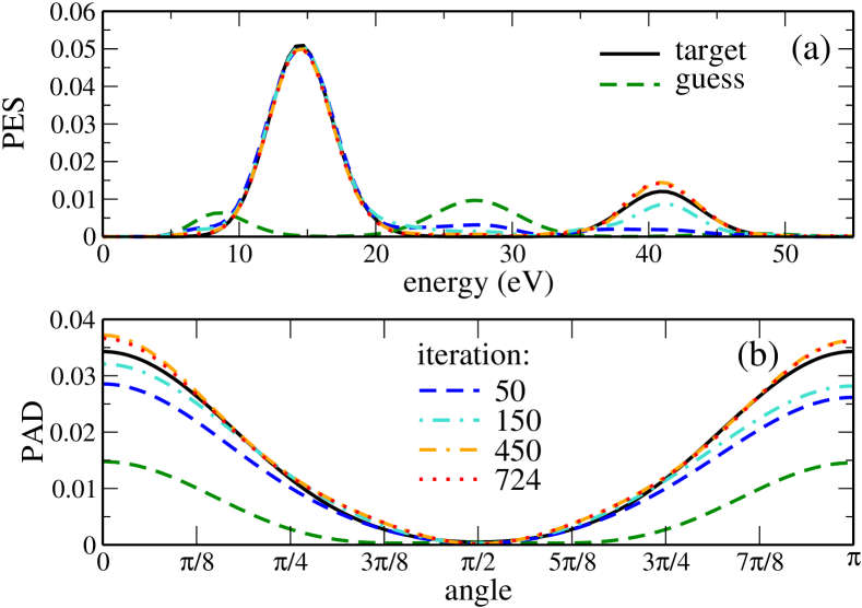
Figure 1: Optimal control of the complete photoelectron distribution for a hydrogen atom: (a) angle-integrated PES, and (b) energy-integrated PAD. As the optimization proceeds iteratively, the actual photoelectron distribution approaches the desired one (black solid line) in both its energy dependence and angular distribution. The photoelectron distribution obtained with the guess field (green dashed lines) is far from the desired distribution.

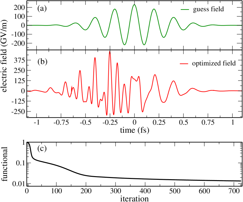
Figure 2: Optimization of the full photoelectron distribution: (a) Guess field $E^{(0)}_{z}(t)$ chosen to start the optimization shown in Fig. 1 and (b) optimized electric field obtained after about 700 iterations. (c) The final time cost functional $J^{(1)}_{T}$ decreases monotonically, as expected for Krotov’s method.

We consider first the minimization of the functional $J^{(1)}[\varphi,\varphi^{\dagger}]$ defined in Eq. (15). The goal is to find a vector potential ${A}_{z,\rm opt}(t)$ such that the photoelectron distribution resulting from the electron dynamics generated by ${A}_{z,\rm opt}(t)$ coincides with $\sigma_{0}(\mathbf{p})$ at every point $\mathbf{p}$, cf. Eq. (15). For visualization convenience, we plot the angle-integrated PES and energy-integrated PAD, cf. Eq. (14), associated to “target” photoelectron distribution $\sigma_{0}(\mathbf{p})$, as shown by the solid-black lines in Figs. 1(a) and 1(b), respectively. To simplify the optimization, neither frequency restriction nor amplitude constraint on ${E}_{z}(t)$ is imposed, i.e., $\lambda_{\omega}=\lambda_{e}=0$. The initial guess for the vector potential is chosen in such a way that the fidelity with respect to the target $\sigma_{0}(\mathbf{p})$ is poor, see the green dashed lines in Fig. 1. Despite the bad initial guess, the optimization quickly approaches the desired photoelectron distribution, converging monotonically, as expected for Krotov’s method and demonstrated in Fig. 2(c): After about 700 iterations, the target distribution is realized with an error of 2%. The reason for such a large number of iterations can be understood by considering that the optimized photoelectron distribution must coincide (point-by-point) with a two-dimensional target object. This represents a non-trivial optimization problem. The optimized electric field is shown in Fig. 2(b): Compared to the initial guess, cf. Fig. 2(a), the amplitude of the optimized field is somewhat increased, and a high-frequency oscillation has been added. The monotonic convergence towards the target distribution in terms of angle-integrated PES and energy-integrated PAD is illustrated in Fig. 1. We can appreciate that the algorithm first tends to match all points with higher values, starting with the peak near 15 eV, while adjusting the remainder of the spectrum, with lower values, later in the optimization. The slow-down of convergence, observed in Fig. 2(c) after about 200 iterations, is typical for optimization methods that rely on gradient information alone: As the optimum is approached, the gradient vanishes Eitan et al. (2011). Such a slow-down of convergence can only be avoided by incorporating information from higher order derivatives in the optimization. This is rather non-trivial in the framework of Krotov’s method Eitan et al. (2011); Jäger et al. (2014) and beyond the scope of our current study.

V Application II: Minimizing the probability of emission into the upper hemisphere

As a second application of our control toolbox, we are interested in minimizing the probability of emission into the upper hemisphere without imposing any specific constraint on the number of electrons emitted into the lower hemisphere. The final time cost functional is given by Eq. (16) with $\lambda_{2}^{+}>0$ and $\lambda_{2}^{-}=0$. We consider again a hydrogen atom and a linearly polarized electric field along the $z$-axis, using the same numerical parameters as in Section IV.

Figure 3: Minimizing, for a hydrogen atom, photoelectron emission into the upper hemisphere: As the optimization proceeds iteratively, the probability of emission into the upper hemisphere decreases monotonically up to almost complete extinction.

.

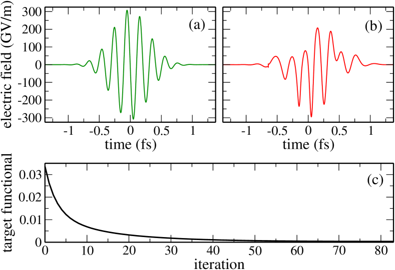
Figure 4: Minimization of the probability of emission into the upper hemisphere for hydrogen: Guess (a) and optimized (b) electric field for the optimization shown in Fig. 3. Also for this target functional, Eq. (16), monotonic convergence of the optimization algorithm is achieved (c).

In contrast to the example discussed in Section IV, no particular expression for the target PES and PAD needs to be imposed—we only require the probability of emission into the upper hemisphere to be minimized regardless of the actual shape of angle-integrated PES and energy-integrated PAD. We employ the optimization prescription described in Section III.2 using Eq. (31c) in the final time condition for the adjoint state. As the optimization proceeds iteratively, the energy-integrated PAD becomes more and more asymmetric, see Fig. 3, minimizing emission into the upper hemisphere, as desired. The guess and optimized pulses are shown in Fig. 4(a) and (b). As illustrated by the solid green line in Fig. 3, the guess field was chosen such that it leads to a symmetric probability of emission for the two hemispheres. Again, monotonic convergence of the final time cost functional is achieved, cf. Fig. 4(c). At the end of the iteration procedure, the probability of emission into the upper hemisphere vanishes completely. As for the lower hemisphere, the emission probability initially remains almost invariant as the algorithm proceeds iteratively, see Fig. 3, while the probability of emission into the upper hemisphere decreases very fast, and monotonically, as expected. However, for a large number of iterations, the probability of emission into the lower hemisphere starts to decrease as well. After about 150 iterations it reaches an emission probability of $2.3\times 10^{-4}$, that is two orders of magnitude smaller than for the guess pulse. Although our goal is only for the probability of emission into the upper hemisphere to be minimized, without specific constraints on the probability of emission into the lower hemisphere, the current results are completely consistent in terms of the optimization problem. More precisely, the optimization does exactly what the functional $J^{(2)}_{T}$, Eq. (16) with $\lambda_{2}^{+}>0$ and $\lambda_{2}^{-}=0$, targets. In fact, since the target functional depends on the upper hemisphere alone, then, by construction, the algorithm calculates the corrections to the field according to Eq. (26), regardless of how these changes affect the probability of emission into the lower hemisphere. To keep the probability of emission into the lower hemisphere constant or to maximize it, an additional optimization functional is required. This is investigated in the following section and defines the motivation for the maximization of the anisotropy of emission discussed in the following lines.

VI Application III: Maximizing the difference in the number of electrons emitted into upper and lower hemisphere

Finally we maximize the difference in probability for emission into the upper and the lower hemispheres. To this end, we construct the final-time cost functional such that it maximizes emission into the upper hemisphere while simultaneously minimizing emission into the lower hemisphere. This is expressed by the functional (16) where both weights are non-zero and have different signs, $\lambda_{2}^{(+)}<0$ and $\lambda_{2}^{(-)}>0$. The signs correspond to maximization and minimization, respectively. We consider this control problem for two different atoms—hydrogen as a one-channel case and argon as an example with three active channels Karamatskou et al. (2014). The latter serves to underline the appropriateness of our methodology for quantum control of multi-channel problems.

Furthermore, in order to demonstrate the versatility of our optimal control toolbox in constraining specific properties of the optimized electric field, we consider the following options: (i) a spectral constraint, i.e., $\lambda_{\omega}\neq 0$ in Eq. (23), and (ii) the constraint to minimize fast changes in the vector potential, with $\lambda_{e}\neq 0$ in Eq. (25). The latter is equivalent to avoiding large electric field amplitudes.

VI.1 Hydrogen

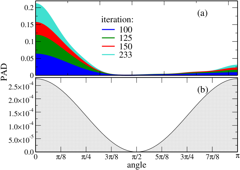
Figure 5: Maximizing, for a hydrogen atom, the difference in photoelectron emission into the upper and lower hemisphere: (a) The probability for emission into the upper hemisphere ($0\leq\theta\leq\pi/2$) increases significantly as the optimization proceeds. Although the probability for emission with angles ($\pi/2\leq\theta\leq\pi$) also grows somewhat, the overall difference increases. The energy-integrated PAD obtained with the guess pulse is shown in (b). Note the different y-axis scales in (a) and (b).

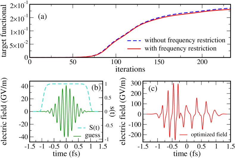
Figure 6: Maximization of the anisotropy in the PAD for hydrogen: The target functional $J_{T}^{(2)}$, for the optimization shown in Fig. 5, measuring the difference in probability for emission into upper and lower hemisphere increases monotonically with ($\lambda_{\omega}\neq 0$) and without ($\lambda_{\omega}=0$) spectral constraint (a). The guess field (green line) is shown in (b) together with the shape function $s(t)$ used in both optimizations. The optimized field obtained with the spectral constraint is displayed in (c).

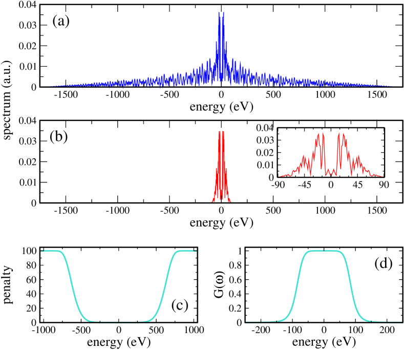
Figure 7: Hydrogen, maximization of the anisotropy of emission: Spectrum of the optimized electric field for the optimization shown in Figs. 5 and 6 with (b) and without (a) spectral constraint. The corresponding penalty function $\tilde{\gamma}(\omega)$ and transfer function $\tilde{G}(\omega)$, cf. Eqs. (23) and (37d), are shown in (c) and (d), respectively.

We consider a hydrogen atom, interacting with an electric field linearly polarized along the $z$-axis, using the same numerical parameters as in Sec. IV. The optimization was carried out with and without restricting the spectral bandwidth of $E_{z}(t)$. Figure 5(b) displays the symmetric energy-integrated PAD obtained with the Gaussian guess field, shown in Fig. 6(b), for which a central frequency $\omega_{0}=27.2\,$eV was used. For the optimization with spectral constraint, the admissible frequency components for $E_{z}(t)$ are chosen such that $\big{|}E_{z}(\omega)\big{|}^{2}\leq\epsilon\,\hskip 2.84544pt\text{for all}\hskip 2.84544pt|\omega|\geq\omega_{max}$ with $\omega_{max}=5\,$a.u.$\,\approx 136.1\,$eV. This requirement translates into the penalty function $\tilde{\gamma}(\omega)$ shown in Fig. 7(c), for which we have used the form

$$\tilde{\gamma}(\omega) = \tilde{\gamma}_{0}\,\left(1-e^{-(\omega/\alpha)^{2n}}\right),$$ (38)

where the parameters $\alpha$, $n$ and $\tilde{\gamma}_{0}$ must be chosen such that the term $\lambda_{\omega}\,\hat{\gamma}(\omega)$ in the functional $C_{\omega}[\mathbf{A}]$ in Eq. (23) takes very large values in the region of undesired frequencies. For our first example, $\alpha=25$, $n=6$ and $\tilde{\gamma}_{0}=1$ allows for strongly penalizing, and therefore filtering all undesirable frequency components above $|\omega|\geq\omega_{max}$, as it is shown by the corresponding transfer function $\tilde{G}(\omega)$, cf. Fig. 7(d). Note that it is not the weight $\lambda_{\omega}$ alone that determines how strictly the spectral constraint is enforced; it is the ratio $\lambda_{\omega}/\lambda_{a}$ that enters in the transfer function $\tilde{G}(\omega)$. This reflects the competition of the different terms in the complete optimization functional, Eq. (18).

As in the previous two examples, the optimization approach developed leads to monotonic convergence of the target functional, Eq. (16), with and without spectral constraint. This is illustrated in Fig. 6(a). Even though the spectra of the fields optimized with and without spectral constraint, are completely different, cf. Fig. 7(a) and (b), the speed of convergence is roughly the same, and the maximum values for $J_{T}^{(2)}$ reached using both fields are also very similar, cf. Fig. 6(a). This means that the algorithm finds two distinct solutions. Such a finding is very encouraging as it implies that the spectral constraint does not put a large restriction onto the control problem. In other words, more than one, and probably many, control solutions exist, and it is just a matter of picking the suitable one with the help of the additional constraint. It also implies that most of the frequency components in the spectrum of the field optimized without spectral constraint are probably not essential. This is verified by removing the undesired spectral components in Fig. 7(a), using the same transfer function utilized for the frequency-constrained optimization shown in Fig. 7(d). The energy-integrated PAD obtained with such a filtered optimized pulse remains asymmetric, and the value of the target functional $J_{T}^{(2)}$ is decreased by only about 10 per cent.

The peak amplitude of the optimized field is about one order of magnitude larger than that of the guess field, cf. Fig. 6(b) and (c). The increase in peak amplitude is connected to the gain in emission probability for the northern hemisphere by almost three orders of magnitude. The optimized pulse thus ionizes much more efficiently than the guess pulse.

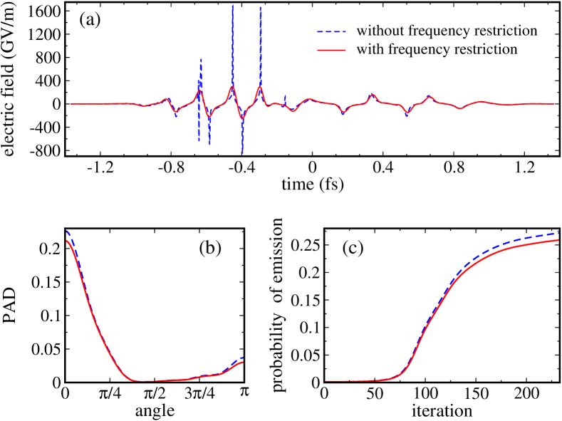
Figure 8: Maximization of the difference of photoelectrons emitted into the lower and upper hemispheres for hydrogen: Optimized electric fields with ($\lambda_{\omega}\neq 0$) and without ($\lambda_{\omega}=0$) frequency restriction (a) where the red curve shows the same data as in Fig. 6(c). Also compared are the energy-integrated PAD (b) and total emission probability (c) obtained with the frequency-constrained and unconstrained optimized fields.

Figure 8(a) compares the electric fields optimized with and without spectral constraints—a huge difference is observed for the two fields. While the electric field optimized without spectral constraint presents very sharp and high peaks in amplitude, beyond experimental feasibility, the frequency-constrained optimized field is characterized by reasonable amplitudes and a much smoother shape. The frequency components of the unconstrained field shown in Fig. 7(a) now become clear. Note that the difference in amplitude only appears during the first half of the overall pulse duration, see Fig. 8(a). It is a known feature of Krotov’s method to favor changes in the field in an asymmetric fashion; the feature results from the sequential update of the control, as opposed to a concurrent one Schirmer and de Fouquieres (2009).

Figure 8(b) shows the energy-integrated PAD obtained upon propagation with the two fields. One notes that, although the probability of emission into the lower hemisphere is larger for the unconstrained than for the constrained field, the same applies to the probability of emission into the upper hemisphere. Therefore the difference in the number of electrons emitted into upper and lower hemisphere is in the end relatively close, which explains the behavior of the final-time functional observed in Fig. 6(a). The electron dynamics generated by the frequency-unconstrained field leads to a larger total probability of emission into both hemispheres, with respect to that obtained with the frequency-constrained field, as shown in Fig. 8(c). More precisely, propagation with the unconstrained optimized field results in a total probability of emission of $0.27$, i.e., probabilities of $0.23$ and $4.3\times 10^{-2}$ for emission into the upper and lower hemisphere, respectively. In comparison, a total probability of emission of $0.26$ is obtained for the frequency-constrained field, with probabilities of emission into the upper and lower hemispheres of $0.22$ and $3.9\times 10^{-2}$, respectively. The fact that the spikes observed in the unconstrained optimized field do not have any significant impact on the asymmetry of the PAD can be rationalized by the short timescale on which the intensity is very high. This time is too short for the electronic system to respond to the rapid variations of the field amplitude.

In order to rationalize how anisotropy of electron emission is achieved by the optimized field, we analyze in Fig. 9 the partial wave decomposition of the angle-integrated PES, comparing the results obtained with the guess field to those obtained with the frequency-constrained optimized field. Inspection of Fig. 9 reveals that upon optimization, there is a clear transition from distinct ATI peaks, Fig. 9(a), to a quasicontinuum energy spectrum, Fig. 9(b). Also, the optimized field enhances the contribution of states of higher angular momentum that have the same kinetic energy. In particular, the peaks for $l=5$ are dramatically higher than in the PES obtained with the guess field. In fact, the symmetric case, cf. Fig. 9(a), shows an energy distribution of partial waves characterized by waves of the same parity at the same energy, whereas the asymmetric case reveals a partial wave distribution of opposite parity at the same energy, cf. Fig. 9(b). Figure 9 thus demonstrates that the desired asymmetry in the energy-integrated PAD is achieved through the mixing of various partial waves of opposite parity at the same energy. Interestingly, especially lower frequencies are mixed with a considerable intensity into the pulse spectrum which leads to higher order multiphoton ionization leading to comparable final energies in the PES. Thus, more angular momentum states are mixed.

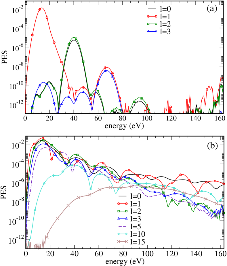
Figure 9: Maximizing the anisotropy of photoelectron emission for hydrogen: Partial wave contribution to the angle-integrated PES, shown in Fig. 5, obtained with the guess (a) and the frequency-constrained optimized field (b).

Next, we would like to constrain not only the frequency components but also the maximal field amplitude, as the maximal field amplitude of the electric field, shown in Fig. 6(c) is still important. To this end, we employ Eq. (37) for $\lambda_{e}>0$, which penalizes large changes on the derivative of the vector potential, cf. Eq. (25), and thus large values of the electric field amplitude. As can be seen in Fig. 10(a), the resulting optimized field is one order of magnitude smaller than that for which no amplitude restriction was imposed, cf. Fig. 6(c), and of the same order of magnitude as the guess field. Despite the constraint and as shown in Fig. 10(c), a perfect top-bottom asymmetry is obtained.

Figure 10: Maximizing the anisotropy of photoelectron emission for hydrogen: Optimization results obtained when simultaneously constraining the maximal amplitude and frequency components of the electric field for the weights $|\lambda^{(-)}_{eff}|=2|\lambda^{(+)}_{eff}|$ with $|\lambda^{(+)}_{eff}|=1$. A perfect anisotropy of emission is obtained.

A common feature observed between the amplitude-unconstrained and constrained cases concerns the low frequencies appearing upon optimization, cf. Fig. 7(b) and Fig. 10(b), respectively. To quantify the role of the frequency components for achieving anisotropy, we start by suppressing all frequency components above $10$ eV: the anisotropy of emission is preserved. On the other hand, removing frequencies below the XUV re-establish the initial symmetry of emission into both hemispheres. Therefore, in both cases the top-bottom asymmetry arises from low frequency components of the optimized field and is achieved through the mixing of various partial waves of opposite parity at the same energy.

VI.2 Argon

We extend now our quantum control multi-channel approach to the study of electron dynamics in argon, interacting with an electric field linearly polarized along the $z$-direction. We consider the $3s$ and $3p$ orbitals to contribute to the ionization dynamics and define three ionization channels $3s$, $3p$ with $m=0$ and $3p$ with $m=+1$ (the case $3p$ with $m=-1$ is symmetric to $m=+1$ due to the polarization direction of the electric field, linearly polarized along to the $z$ axis). In order to describe the multi-channel dynamics, a spatial grid of $100\,$a.u. with $450$ grid points and a density parameter of $\zeta=0.55$ was utilized. The size of the radial component of the spherical momentum grid was set to $E_{max}=12\,$a.u., sampled by $601$ evenly spaced points, while the polar component $\theta\in[0,\pi]$ was discretized using $301$ points. A splitting radius of $r_{c}=50\,$ a.u., and a smoothing parameter $\Delta=10.0\,$a.u. were employed, together with a splitting step of $2.0\,$a.u. and a total number of $N_{s}=2036$ splitting times. For time propagation, the time step was chosen to be $0.01\,$a.u., for an overall integration time $\Delta T\approx 200\,$a.u.

Figure 11: Maximizing, for an argon atom, the difference in photoelectron emission into the upper and lower hemisphere: Guess field (a) utilized for the optimization. Optimized fields obtained with an amplitude constraint are depicted in (b) and (c) respectively.

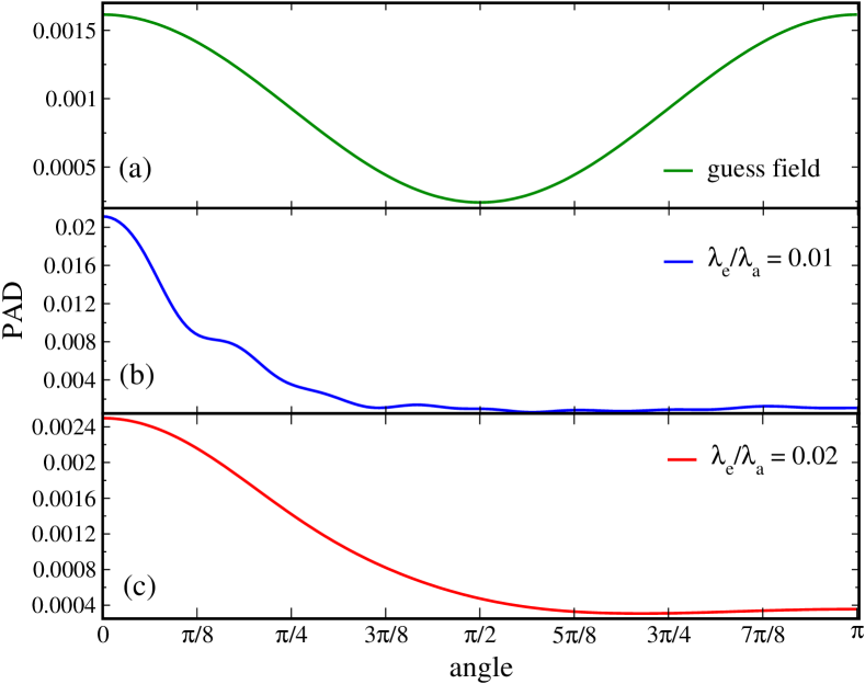
Figure 12: Maximization of the top-bottom asymmetry in argon: Energy-integrated PAD obtained with the guess pulse (a) and amplitude-constrained cases with $|\lambda^{(-)}_{eff}|=2|\lambda^{(+)}_{eff}|$ and $|\lambda^{(+)}_{eff}|=1$ in (b) and (c), respectively. Note the different scales for the probability of emission.

Analogously to the results shown for hydrogen in Sec. VI.1, the goal is to maximize the difference in the probability for electron emission into the upper and lower hemispheres. To start the optimization, a Gaussian-shaped guess electric field with central frequency $\omega=27.2\,$eV and maximal amplitude $E_{max}=5.14\,$GV/m was chosen. It is depicted in Fig. 11(a) and yields a symmetric distribution for the upper and lower hemispheres, see Fig. 12(a). The total emission probability amounts to only $1.4\times 10^{-2}$. In order to obtain reasonable pulses which result in a maximally anisotropic PAD, we utilize Eq. (25) with $\lambda_{e}\neq 0$ to minimize fast changes in the vector potential and avoid large peaks of the electric field amplitude.

The optimized pulses for two values of the ratio $\lambda_{e}/\lambda_{a}$, charaterizing the relative weight of minimizing peak values in the electric field compared to minimizing the integrated vector potential, are shown in Figs. 11(b) and (c), respectively. As expected, a larger amplitude constraint yields an electric field with a smaller maximal amplitude. In fact, the maximal amplitude for $\lambda_{e}/\lambda_{a}=0.01$ is one order of magnitude larger than that of the guess field, whereas for $\lambda_{e}/\lambda_{a}=0.02$ it is only three times larger. Figures 12(b) and (c) display the energy-integrated PADs obtained with these fields. A significant top-bottom asymmetry of emission is achieved in both cases, the main difference being the total emission probability of $2.7\times 10^{-2}$ for Fig. 12(b) compared to $9.4\times 10^{-3}$ for Fig. 12(c). The spectra of the two optimized fields are examined in Fig. 13. Despite the difference in amplitude, both optimized fields are characterized by low frequency components. Note that no frequency restriction was imposed. This finding suggests that the low frequency components are responsible for achieving the top-bottom asymmetry. Indeed, removing all optical and infra-red (IR) components results in a complete loss of the asymmetry. On the other hand, removing frequency components above $10\,$eV does not affect the top-bottom asymmetry achieved by both optimized fields considerably.

Figure 13: Anisotropy of PAD in argon: Spectra of the optimized pulses and the guess field for comparison.

These optimization results raise the question whether frequency components in the optical and IR range are essential for achieving the top-bottom asymmetry or whether a pure XUV field can also realize the desired control. To answer this question, we now penalize all frequency components in the optical and IR region. The resulting optimized electric field and its spectrum are depicted in Fig. 14(a) and (b), respectively. This field indeed possesses frequency components only in the XUV region, cf. Fig. 14(b). Nevertheless, a strongly asymmetric top-bottom emission is again achieved, cf. Fig. 14(c). Therefore, while optical or IR excitation may significantly contribute to achieving anisotropy of the photoelectron emission, fields with frequency components in the XUV alone may also lead to such an asymmetry.

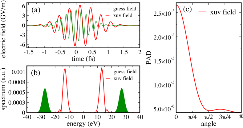
Figure 14: Top-bottom asymmetry in argon: Frequency and amplitude-constrained optimized field and its spectrum in (a) and (b) with the guess field shown for comparison. For obtaining the XUV field, the ratios $\lambda_{e}/\lambda_{a}=0.02$ and $\lambda_{\omega}/\lambda_{a}=0.02$ with a penalty function $\tilde{\gamma}_{XUV}=\tilde{\gamma}(\omega-\omega_{0})+\tilde{\gamma}(\omega+\omega_{0})-1+\epsilon_{\omega}$ with $\tilde{\gamma_{o}}=100$, $\omega_{0}=27.2$ eV, $n=4$ and $\alpha=15$ were utilized, cf. Eq. (38). The quantity $\epsilon_{\omega}=0.001$ has been introduced in order to avoid numerical instabilities when evaluating the transfer function $\tilde{G}(\omega)$, cf. Eq. (37d).

Finally, we would like to understand the physical mechanism from which the anisotropy in the emission into both hemispheres arises. To this end, we consider the partial wave decomposition of the angle-integrated PES. Analogously to our analysis for hydrogen, cf. Section VI.1, a symmetric PAD, as obtained with the guess field, is characterized by an energy distribution of partial waves of the same parity at the same energy, cf. Fig. 15(a). In contrast, the partial wave decomposition corresponding to the asymmetric PAD reveals an energy distribution of partial waves of different parity at the same energy, cf. Figs. 15(b), 16(a). For the optimized fields with significant optical and IR components, many partial waves, including those with high angular momentum, contribute to the angle-integrated PES. This suggests that the top-bottom anisotropy of photoelectron emission is achieved by absorbing low-energy photons at relatively high intensity which is accompanied by strong mixing of a number of partial waves of opposite parity at the same energy. The same mechanism had previously been found for hydrogen, cf. Section VI.1.

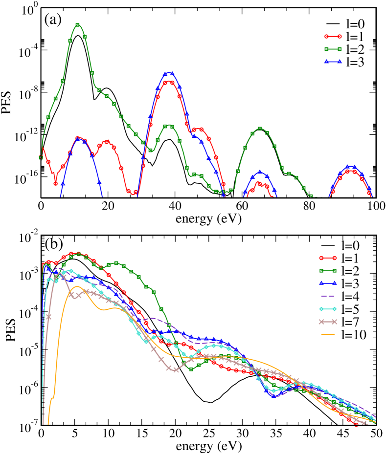
Figure 15: Maximizing the anisotropy of photoelectron emission for argon: Partial wave contribution to the angle-integrated PES, shown in Fig. 12 obtained with the guess (a) and the amplitude-constrained optimized field corresponding to the ratio $\lambda_{e}/\lambda_{a}=0.01$ in (b).

Figure 16: Maximizing the anisotropy of photoelectron emission for argon: Partial wave contributions to the angle-integrated PES corresponding to the energy-integrated PAD shown in Fig. 12(c) obtained amplitude-constrained optimized field for the ratio $\lambda_{e}/\lambda_{a}=0.02$ and that corresponding to the PAD shown in Fig. 14(c) obtained with the optimized XUV pulse in pannels (a) and (b), respectively.

As for the optimized XUV electric field yielding an asymmetric probability for emission, shown in Fig. 14(c), the same mechanism involving mixing of partial waves of different parity at the same energy is found, cf. Fig. 16(b). Nevertheless, a much smaller number of partial waves is involved, cf. Fig. 16(a) and (b). For the XUV pulse (Fig. 14(b)), it is mainly the components of the continuum wavefunction with angular momentum $l=2$ and $l=3$ that contribute to the anisotropy of emission.

The reason why partial waves with different parity are always present for anisotropic photoelectron emission can be straightforwardly understood. It lies in the fact that the angular distribution arises from products of spherical harmonics, cf. Eqs. (14a), (13) and (9), and the product of two spherical harmonics with the same (opposite) parity is a symmetric (antisymmetric) function of $\theta$. The optimized pulses take advantage of this property and realize the desired asymmetry by driving the dynamics in such a way that it results in partial wave components which interfere constructively (destructively) in the upper (lower) hemisphere.

We have also investigated whether channel coupling plays a role in the generation of the anisotropy. While switching off the interchannel coupling in the dynamics under the optimized pulse shown in Fig. 14(a) decreases the resulting anisotropy slightly, overall it still yields an anisotropic PAD. This shows that interchannel coupling in argon is not a key factor in achieving top-bottom asymmetry in photoelectron angular distributions.

VII Conclusions

To summarize, we have developed a quantum optimal control toolbox to target specific features in photoelectron spectra and photoelectron angular distributions that result from the interaction of a closed-shell atom with strong XUV radiation. To this end, we have combined Krotov’s method for quantum control Reich et al. (2012) with the time-dependent configuration interaction singles approach to treat the electron dynamics Greenman et al. (2010) and the wave-function splitting method to calculate photoelectron spectra Karamatskou et al. (2014, 2015). We have presented here the algorithm and its implementation in detail. To the best of our knowledge, our work is the first to directly target photoelectron observables in quantum optimal control.

We have utilized this toolbox to identify, for the benchmark systems of hydrogen and argon atoms, photoionization pathways which result in asymmetric photoelectron emission. Our optimization results show that efficient mechanisms for achieving top-bottom asymmetry exist in both single-channel and multi-channel systems. We have found the channel coupling to be beneficial, albeit not essential for achieving asymmetric photoelectron emission. Since typically the solution to a quantum control problem is not unique, additional constraints are useful to ensure certain desired properties of the control fields, such as limits to peak amplitude and spectral width. We have demonstrated how such constraints allow to determine solutions characterized by low or high photon frequency. In the low frequency regime, our control solutions require relatively high intensities. Correspondingly, the anisotropy of the photoelectron emission is realized by strong mixing of many partial waves. In contrast, for pure XUV pulses, we have found low to moderate peak amplitudes to be sufficient for asymmetric photoelectron emission. In both cases, we have identified the top-bottom asymmetry to originate from mixing, in the photoelectron wavefunction, various partial waves of opposite parity at the same energy. The corresponding constructive (destructive) interference pattern in the upper (lower) hemisphere yields the desired asymmetry of photoelectron emission. Whereas many partial waves contribute for control fields characterized by low photon energy and high intensity, interference of two partial waves is found to be sufficient in the pure XUV regime. In all our examples, we have found surprisingly simple shapes of the optimized electric fields. In the case of hydrogen, tailored electric fields to achieve asymmetric photoelectron emission have been discussed before and we can compare our results to those of Refs. Chelkowski et al. (2004); Shvetsov-Shilovski et al. (2014). Our work differs from these studies in that we avoid a parametrization of the field and allow for complete freedom in the change the electric field, whereas Refs. Chelkowski et al. (2004); Shvetsov-Shilovski et al. (2014) considered only the carrier-envelope phase, intensity and duration of the pulse as control knobs. The additional freedom of quantum optimal control theory is important, in particular when more complex systems are considered.

The set of applications that we have presented here is far from being exhaustive, and our current work opens many perspectives for both photoionization studies and quantum optimal control theory. On the one hand, we have shown how to develop optimization functionals that target directly an experimentally measurable quantity obtained from continuum wavefunctions. On the other hand, since our approach is general, it can straightforwardly be applied to more complex examples. In this respect it is desirable to lift the restriction to closed-shell systems. This would pave the way to studying the role of electron correlation in maximizing certain features in the photoelectron spectrum. Similarly, allowing for circular or elliptic polarization of the electric field, one could envision, for example, to maximize signatures of chirality in the photoelectron angular distributions. This requires, however, substantial further development on the level of the time-dependent electronic structure theory.

Appendix A Frequency and Amplitude Restriction

In the following, we present the derivation of Krotov’s update equation for the control, Eq. (26) using the approximation for $s(t)$ previously described. This allows for a more compact expression for Krotov’s equation for the specific constraints on the field used in this work. It is obtained following Ref. Reich et al. (2012): We seek to minimize the complete functional, Eq. (18). In order to evaluate the extremum condition, we start by evaluating the functional derivative of the penalty functional with respect to the changes in the control field $\mathbf{A}(t)$ in Eq. (22),

$$\dfrac{\delta C_{a}[\mathbf{A}]}{\delta\mathbf{A}(t)} = 2\lambda_{a}s^{-1}(t)\left(\mathbf{A}(t)-\mathbf{A}_{\rm ref}(t)\right).$$ (39)

Next, we evaluate the functional derivative of Eq. (23). Abbreviating $\omega^{2}\tilde{\gamma}(\omega)$ by $\tilde{h}(\omega)$ in Eq. (23), the functional derivative reads

$$\dfrac{\delta C_{\omega}[\mathbf{A}]}{\delta\mathbf{A}(t)} = \lambda_{\omega}\int\mathbf{A}^{\star}(\omega)\dfrac{\delta\tilde{\mathbf{A}}(\omega)}{\delta\mathbf{A}(t)}\tilde{h}(\omega)\,d\omega$$ (40)

$$+\lambda_{\omega}\int\tilde{\mathbf{A}}(\omega)\dfrac{\delta\tilde{\mathbf{A}}^{\star}(\omega)}{\delta\mathbf{A}(t)}\tilde{h}(\omega)\,d\omega\,.$$

Using the fact that $\tilde{\mathbf{A}}(\omega)$ is the Fourier transform of $\mathbf{A}(t)$,

$$\tilde{\mathbf{A}}(\omega)=\int\mathbf{A}(t)e^{-i\omega t}\,dt\,,$$

the functional derivative becomes,

$$\dfrac{\delta\tilde{\mathbf{A}}(\omega)}{\delta\mathbf{A}(t^{\prime})}=e^{-i\omega t^{\prime}}\,,$$

such that

$$\dfrac{\delta C_{\omega}[\mathbf{A}]}{\delta\mathbf{A}(t)} = \lambda_{\omega}\int\tilde{\mathbf{A}}^{\star}(\omega)e^{-i\omega t}\tilde{h}(\omega)\,d\omega$$

$$+\lambda_{\omega}\int\tilde{\mathbf{A}}(\omega)e^{+i\omega t}\tilde{h}(\omega)\,d\omega\,\,.$$

This can be rewritten as

$$\dfrac{\delta C_{\omega}[\mathbf{A}]}{\delta\mathbf{A}(t)} = \lambda_{\omega}\int\tilde{\mathbf{A}}^{\star}(-\omega)e^{+i\omega t}\tilde{h}(-\omega)\,d\omega$$ (41)

$$+\lambda_{\omega}\int\tilde{\mathbf{A}}(\omega)e^{+i\omega t}\tilde{h}(\omega)\,d\omega\,.$$

Since the control $\mathbf{A}(t)$ is a real function of time, $\tilde{\mathbf{A}}^{\star}(-\omega)=\tilde{\mathbf{A}}(\omega)$. Moreover, by construction $\tilde{h}(\omega)=\tilde{h}(-\omega)$. Therefore, Eq. (41) becomes

$$\dfrac{\delta C_{\omega}[\mathbf{A}]}{\delta\mathbf{A}(t)} = 2\lambda_{\omega}\int\tilde{\mathbf{A}}(\omega)e^{+i\omega t}\tilde{h}(\omega)\,d\omega$$

$$= 2\lambda_{\omega}\int\tilde{\mathbf{A}}(\omega)e^{i\omega t}d\omega\int h(\tau)e^{-i\omega\tau}\,d\tau$$

$$= 2\lambda_{\omega}\int h(\tau)d\tau\int\tilde{\mathbf{A}}(\omega)e^{+i\omega(t-\tau)}d\omega$$

$$= 2\tilde{\lambda}_{\omega}\int h(\tau)\mathbf{A}(t-\tau)d\tau=2\tilde{\lambda}_{\omega}\mathbf{A}\star h(t)\,,$$

with $\tilde{\lambda}_{\omega}=\sqrt{2\pi}\lambda_{\omega}$, and $h(t)=\int{\tilde{h}(\omega)\exp{(+i\omega t})}\,d\omega/\sqrt{2\pi}$ and where $f\star g(t)$ refers to the convolution product of $f$ and $g$.

We now calculate the functional derivative of the constraint penalizing large values of $\dot{\mathbf{A}}(t)$, Eq. (25). Assuming vanishing boundary conditions for $\mathbf{A}(t)$, we find, upon integration by parts,

$$\dfrac{\delta C_{e}[\mathbf{A}]}{\delta\mathbf{A}(t)} = -2\lambda_{e}s^{-1}(t)\ddot{\mathbf{A}}(t)\,.$$ (43)

Using Eqs. (39), (A) and (43), the extremum condition with respect to a variation in the control becomes

$$0 = \lambda_{a}\,s^{-1}(t)\left(\mathbf{A}(t)-\mathbf{A}_{ref}(t)\right)-\lambda_{e}\,s^{-1}(t)\ddot{\mathbf{A}}(t)$$

$$+\tilde{\lambda}_{\omega}\,\mathbf{A}\star h(t)-\mathfrak{Im}\left\{\left\langle\chi(t)\left|\frac{\partial\hat{H}}{\mathbf{A}}\right|\Psi(t)\right\rangle\right\}\,.$$

where the last term has been previously introduced in Eq. (26). It can be straightforwardly derived from variational principles, ie. Euler-Lagrange Lagrange equation, or in the context of Pontriagin’s maximum/minimum principle or in the context of Krotov’s optimization method, cf. Refs. Reich et al. (2012, 2014). It stresses the dynamics to which the forward propagated state is subject to. Solving for $\mathbf{A}(t)$ gives us the update rule for the optimized pulse,

$$\mathbf{A}(t) = \mathbf{A}_{ref}(t)+\frac{s(t)}{\lambda_{a}}\,\mathfrak{Im}\left\{\left\langle\chi(t)\left|\frac{\partial\hat{H}}{\mathbf{A}}\right|\Psi(t)\right\rangle\right\}$$ (44)

$$-\frac{\tilde{\lambda}_{\omega}}{\lambda_{a}}s(t)\mathbf{A}\star h(t)+\frac{\lambda_{e}}{\lambda}_{a}\ddot{\mathbf{A}}(t)\,,$$

i.e., we retrieve Eq. (26). Using the property

$$\int\ddot{\mathbf{A}}(t)\,e^{-i\omega\,t}\,dt=-\omega^{2}\,\tilde{\mathbf{A}}(\omega)\,,$$

together with Eq. (36) for $s(t)$, it is straighforward to write Krotov’s equation in frequency domain. To this end, we merely take the Fourier transform of Eq. (44) and utilize the well-known property that the Fourier transform of a convolution of two functions in time domain is the product of the functions in frequency domain. We thus find

$$\tilde{\mathbf{A}}^{(k+1)}(\omega) \approx \tilde{\mathbf{A}}^{(k)}(\omega)+\tilde{I}^{(k+1)}(\omega)$$

$$-\frac{\tilde{\lambda}_{\omega}}{\lambda_{a}}\tilde{\mathbf{A}}^{(k+1)}(\omega)\tilde{h}(\omega)-\omega^{2}\frac{\lambda_{e}}{\lambda_{a}}\tilde{\mathbf{A}}^{(k+1)}(\omega)\,,$$

which yields Eq. (37a).

References

- Hüfner (2003) S. Hüfner, Photoelectron Spectroscopy, Principles and Applications (Springer, 2003), 3rd ed.
- Meyer et al. (2010) M. Meyer, D. Cubaynes, V. Richardson, J. T. Costello, P. Radcliffe, W. B. Li, S. Düsterer, S. Fritzsche, A. Mihelic, K. G. Papamihail, et al., Phys. Rev. Lett. 104, 213001 (2010).
- Fabre et al. (1981) F. Fabre, P. Agostini, G. Petite, and M. Clement, Journal of Physics B: Atomic and Molecular Physics 14, L677 (1981).
- Becker and Shirley (1996) U. Becker and D. A. Shirley, VUV and Soft X-Ray Photoionization (Springer Science & Business Media, 1996), 3rd ed.
- Wu et al. (2011) G. Wu, P. Hockett, and A. Stolow, Phys. Chem. Chem. Phys. 13, 18447 (2011).
- Blaga et al. (2009) C. I. Blaga, F. Catoire, P. Colosimo, G. G. Paulus, H. G. Muller, P. Agostini, and L. DiMauro, Nature Phys. 5, 335 (2009).
- Krausz and Ivanov (2009) F. Krausz and M. Ivanov, Rev. Mod. Phys. 81, 163 (2009).
- Wabnitz et al. (2002) H. Wabnitz, L. Bittner, A. R. B. de Castro, R. Dohrmann, P. Gurtler, T. Laarmann, W. Laasch, J. Schulz, A. Swiderski, K. von Haeften, et al., Nature Physics 420, 482 (2002).
- Corkum and Krausz (2007) P. Corkum and F. Krausz, Nature Physics 3, 381 (2007).
- Kanter et al. (2011) E. P. Kanter, B. Krässig, Y. Li, A. M. March, P. Ho, N. Rohringer, R. Santra, S. H. Southworth, L. F. DiMauro, G. Doumy, et al., Phys. Rev. Lett. 107, 233001 (2011).
- Schwarz (1980) H. E. Schwarz, Journal of Electron Spectroscopy and Related Phenomena 21 (1980).
- Duinker (1982) P. Duinker, Rev. Mod. Phys. 54, 325 (1982).
- Reid (2003) K. L. Reid, Annu. Rev. Phys. Chem. 54, 397 (2003).
- Meier and Engel (1994) C. Meier and V. Engel, Phys. Rev. Lett. 73, 3207 (1994).
- Shen and Engel (2002) Z. Shen and V. Engel, Chem. Phys. Lett. 358, 344 (2002).
- Wollenhaupt et al. (2005) M. Wollenhaupt, V. Engel, and T. Baumert, Annu. Rev. Phys. Chem. 56, 25 (2005).
- Gräfe et al. (2005) S. Gräfe, M. Erdmann, and V. Engel, Phys. Rev. A 72, 013404 (2005).
- Braun et al. (2014) H. Braun, T. Bayer, C. Sarpe, R. Siemering, R. de Vivie-Riedle, T. Baumert, and M. Wollenhaupt, J. Phys. B 47, 124015 (2014).
- Reich et al. (2012) D. M. Reich, M. Ndong, and C. P. Koch, J. Chem. Phys. 136, 104103 (2012).
- Greenman et al. (2010) L. Greenman, P. J. Ho, S. Pabst, E. Kamarchik, D. A. Mazziotti, and R. Santra, Phys. Rev. A 82, 023406 (2010).
- Karamatskou et al. (2014) A. Karamatskou, S. Pabst, Y.-J. Chen, and R. Santra, Phys. Rev. A 89, 033415 (2014).
- Karamatskou et al. (2015) A. Karamatskou, S. Pabst, Y.-J. Chen, and R. Santra, Phys. Rev. A 91, 069907 (2015).
- Klamroth (2006) T. Klamroth, J. Chem. Phys. 124, 144310 (2006).
- Mundt and Tannor (2009) M. Mundt and D. J. Tannor, New J. Phys. 11, 105038 (2009).
- Castro et al. (2012) A. Castro, J. Werschnik, and E. K. U. Gross, Phys. Rev. Lett. 109, 153603 (2012).
- Hellgren et al. (2013) M. Hellgren, E. Räsänen, and E. K. U. Gross, Phys. Rev. A 88, 013414 (2013).
- McCurdy and Rescigno (1997) C. W. McCurdy and T. N. Rescigno, Phys. Rev. A 56, R4369 (1997).
- Martín (1999) F. Martín, Journal of Physics B: Atomic, Molecular and Optical Physics 32, R197 (1999).
- Rescigno and McCurdy (2000) T. N. Rescigno and C. W. McCurdy, Phys. Rev. A 62, 032706 (2000).
- Bachau et al. (2001) H. Bachau, E. Cormier, P. Decleva, J. E. Hansen, and F. Martín, Reports on Progress in Physics 64, 1815 (2001).
- McCurdy and Martín (2004) C. W. McCurdy and F. Martín, Journal of Physics B: Atomic, Molecular and Optical Physics 37, 917 (2004).
- Greenman et al. (2014) L. Greenman, C. P. Koch, and K. B. Whaley, Phys. Rev. A 92, 013407 (2015).
- Rathje et al. (2013) T. Rathje, A. M. Sayler, S. Zeng, P. Wustelt, H. Figger, B. D. Esry, and G. G. Paulus, Phys. Rev. Lett. 111, 093002 (2013).
- Shvetsov-Shilovski et al. (2014) N. I. Shvetsov-Shilovski, E. Räsänen, G. G. Paulus, and L. B. Madsen, Phys. Rev. A 89 (2014).
- Pabst et al. (Rev 1425, 2014) S. Pabst, L. Greenman, and R. Santra, XCID program package for multichannel ionization dynamics (Rev 1425, 2014).
- Leforestier et al. (1991) C. Leforestier, R. Bisseling, C. Cerjan, M. Feit, R. Friesner, A. Guldberg, A. Hammerich, G. Jolicard, W. Karrlein, H.-D. Meyer, et al., J. Comput. Phys. 94, 59 (1991).
- Kosloff (1994) R. Kosloff, Annu. Rev. Phys. Chem. 45, 145 (1994).
- Rohringer et al. (2006) N. Rohringer, A. Gordon, and R. Santra, Phys. Rev. A 74, 043420 (2006).
- Tong et al. (2006) X. M. Tong, K. Hino, and N. Toshima, Phys. Rev. A 74, 031405 (2006).
- Palao et al. (2013) J. P. Palao, D. M. Reich, and C. P. Koch, Phys. Rev. A 88, 053409 (2013).
- Reich et al. (2014) D. M. Reich, J. P. Palao, and C. P. Koch, J. Mod. Opt. 61, 822 (2014).
- Hohenester et al. (2007) U. Hohenester, P. K. Rekdal, A. Borzì, and J. Schmiedmayer, Phys. Rev. A 75, 023602 (2007).
- Palao and Kosloff (2003) J. P. Palao and R. Kosloff, Phys. Rev. A 68, 062308 (2003).
- Eitan et al. (2011) R. Eitan, M. Mundt, and D. J. Tannor, Phys. Rev. A 83, 053426 (2011).
- Jäger et al. (2014) G. Jäger, D. M. Reich, M. H. Goerz, C. P. Koch, and U. Hohenester, Phys. Rev. A 90, 033628 (2014).
- Schirmer and de Fouquieres (2009) S. G. Schirmer and P. de Fouquieres, New J. Phys. 13, 073029 (35pp) (2009).
- Schröder and Brown (2009) M. Schröder and A. Brown, New J. Phys. 11, 105031 (13pp) (2009).
- Lapert et al. (2009) M. Lapert, R. Tehini, G. Turinici, and D. Sugny, Phys. Rev. A 79, 063411 (2009).
- Chelkowski et al. (2004) S. Chelkowski, A. D. Bandrauk, and A. Apolonski, Phys. Rev. A 70, 013815 (2004).