The Dust Attenuation Curve versus Stellar Mass for Emission Line Galaxies at $z\sim 2$

Abstract

We derive the mean wavelength dependence of stellar attenuation in a sample of 239 high redshift ($1.90<z<2.35$) galaxies selected via Hubble Space Telescope (HST) WFC3 IR grism observations of their rest-frame optical emission lines. Our analysis indicates that the average reddening law follows a form similar to that derived by Calzetti et al. for local starburst galaxies. However, over the mass range $7.2\lesssim\log M/M_{\odot}\lesssim 10.2$, the slope of the attenuation law in the UV is shallower than that seen locally, and the UV slope steepens as the mass increases. These trends are in qualitative agreement with Kriek & Conroy, who found that the wavelength dependence of attenuation varies with galaxy spectral type. However, we find no evidence of an extinction “bump” at 2175 Å in any of the three stellar mass bins, or in the sample as a whole. We quantify the relation between the attenuation curve and stellar mass and discuss its implications.

1. Introduction

One of the most important uncertainties associated with the interpretation of high-redshift galaxy observations is our lack of understanding about interstellar extinction. Measurements of galactic star formation rates (SFRs), mass-specific star formation rates (sSFR), age, metallicity, and size all depend in some way on the assumed wavelength dependence and normalization of the dust attenuation law, yet our knowledge of reddening and extinction remains quite limited. From observations of the local universe, it is clear that reddening curves are not universal: while most sight-lines in the Milky Way (MW) have a strong extinction bump near 2175 Å (Stecher, 1965; Cardelli et al., 1989), the feature is weaker in the Large Magellanic Cloud (LMC; Koornneef & Code, 1981) and largely absent in the Small Magellanic Cloud (SMC; Prevot et al., 1984). This diversity is also reflected by systematic changes in the far ultraviolet (UV), where the wavelength dependence of extinction steepens dramatically as one goes from the Milky Way to the SMC.

Further complicating the issue is the fact that dust within a galaxy is spatially distributed, so simple screen models do not apply to observations of integrated galactic light. As first reported by Charlot & Fall (2000), patchy absorption that is distributed throughout a galaxy can result in an effective attenuation law that has a much weaker wavelength dependence than that measured for stars in the Milky Way or Magellanic Clouds. Indeed, by observing 39 nearby starburst systems, Calzetti et al. (1994, 2000) defined an attenuation law between 1200 Å and 6300 Å  that is much shallower than any screen model, and that has a notable absence of the 2175 Å bump.

This Calzetti et al. (2000) law, of course, is an empirical relation which averages over much of the galactic physics that affects the reddening curve. Consider that all young stars spend the first 2 or 3 Myr of their lives enshrouded in dusty molecular clouds (Lada & Lada, 2003). The dust eventually disperses, so by the time the stars are $\sim 100$ Myr old, they have become dynamically mixed among the older populations. As a result, one often models a galaxy’s dust attenuation law with two separate components: an optically thin term that is applicable to the older stars, and a dense, optically thick birth cloud that attenuates younger objects (e.g., Silva et al., 1998; Charlot & Fall, 2000). Using the dust models of Silva et al. (1998), Granato et al. (2000) showed that this age dependency plays a role in defining a galaxy’s net attenuation. In systems dominated by young stars embedded in molecular clouds (i.e., starburst galaxies), a shallower UV attenuation curve is found, and no 2175 Å bump is visible. Conversely, in more “normal” star-forming galaxies, where a significant fraction of UV photons are emitted by stars that are no longer in their birth clouds, the wavelength dependence is steeper, and there is evidence for excess extinction at 2175 Å. Other studies support this model, demonstrating that the 2175 Å bump is typically visible in “normal” star-forming galaxies (e.g., Burgarella et al., 2005; Conroy et al., 2010), but not in starburst systems (Calzetti et al., 1994).

In practice, age and population dependencies are rarely considered when applying dust attenuation to distant galaxies. Instead, the simple Calzetti et al. (2000) attenuation law, without a 2175 Å bump, is most often used to de-redden galactic spectrophotometry in the $z\gtrsim 2$ universe (e.g., Bouwens et al., 2009; Finkelstein et al., 2015). Such an application can be justified by the fact that many of these distant systems have star-formation rates similar to today’s most extreme starburst galaxies. But how reliable is this curve? A number of $z\gtrsim 1$ studies have presented evidence that contradicts the Calzetti et al. (2000) law (Buat et al., 2011, 2012; Scoville et al., 2015), observing both a 2175 Å bump and a steeper wavelength dependence in the UV, and Reddy et al. (2015) has argued that, while the attenuation curve may agree with Calzetti et al. (2000) at $\lambda<2500$ Å, it more closely follows an SMC extinction curve at longer wavelengths. Moreover, the attenuation curve at high redshift may not be universal. Kriek & Conroy (2013) report that, for bright ($R<25$), composite-spectrum galaxies with photometric redshifts between $0.5<z<2.0$, H$\alpha$ equivalent widths correlate inversely with the strength of the 2175 Å bump and the slope of the UV reddening law. Similarly, by examining subgroups of 751 galaxies between $0.9<z<2.2$, Buat et al. (2012) found that the strength of 2175 Å bump was independent of SFR, but was a weak function of stellar mass and specific star formation rate.

To make further progress on this question, large samples of galaxies are needed with well-defined redshifts, comprehensive rest-frame UV through far-IR photometry, intrinsic spectral energy distributions (SEDs) that are reasonably well known, and stellar masses and star formation rates that span a large dynamic range. Such samples now exist in the GOODS (Giavalisco et al., 2004) and COSMOS (Scoville et al., 2007) fields, thanks to a combination of HST infrared grism spectroscopy (Brammer et al., 2012; Weiner et al., 2014), HST high-resolution imaging, and a large database of broad- and intermediate-band photometry (Skelton et al., 2014). Using these data, it is possible to investigate the redshift dependence of dust attenuation and emission in a self-consistent manner, taking into account variations in the underlying stellar population and information regarding galactic orientation (H. Brooks et al., 2016, in preparation). Unfortunately, such an analysis comes at a cost: to compute these properties and derive realistic uncertainties, one needs to consider a large number of parameters. Here, we take a more limited approach, and, following the strategy taken by Scoville et al. (2015), consider only the effects of dust attenuation in a subset of $z\sim 2$ galaxies with intense star formation. Specifically, by selecting galaxies with strong emission lines, we limit our analysis to objects whose intrinsic rest-frame UV SEDs are only weakly sensitive to the details of the stellar population (Calzetti, 2001). Moreover, by including only sources with at least two emission features, we ensure that the redshift assigned to each object is unambiguous.

In this paper, we derive the mean empirical reddening curve for a sample of $1.9<z<2.35$ galaxies selected via the luminosity of their rest-frame optical emission lines and quantify how the properties of this curve change as a function of stellar mass. This will lay the groundwork for a more in depth analysis which will self-consistently examine the reddening curves of individual $z\sim 2$ systems (H. Brooks et al., 2016, in preparation). In §2, we define our sample, briefly describe our modeling of the galaxies’ spectral energy distributions, and outline the procedures used to measure the objects’ stellar masses and star formation rates. In this section, we also show that the UV SEDs of our objects can be well-matched using constant star-formation stellar population models with ages between 10 Myr and 500 Myr. In §3 we create our database of photometric observations by interpolating in the PSF-matched photometry catalog of Skelton et al. (2014), and in §4 we use these data to derive a mean attenuation curve for our sample of emission-line galaxies. The primary result of this paper is then given in §5, where we describe how the mean attenuation curve varies with stellar mass, and present a prescription for correcting $z\sim 2$ emission-line galaxies for the effects of internal stellar reddening. We conclude by discussing the implications of our measurements.

For this paper, we assume a $\Lambda$CDM cosmology, with $\Omega_{\Lambda}=0.7$, $\Omega_{M}=0.3$ and $H_{0}=70$ km s^-1 Mpc^-1 (Hinshaw et al., 2013).

2. The Sample

To perform our analysis, we used a sample of $z\sim 2$ galaxies observed in the GOODS-N, GOODS-S, and COSMOS regions with the G141 near-IR grism of the Hubble Space Telescope’s Wide Field Camera 3. This dataset, which was taken as part of the 3D-HST (Brammer et al., 2012) and AGHAST (Weiner et al., 2014) surveys (GO programs 11600, 12177, and 12328), consists of $R\sim 130$ slitless spectroscopy over the wavelength range $1.08~{}\mu{\rm m}<\lambda<1.68~{}\mu$m, and records total emission line fluxes over 350 arcmin² of sky. Tens of thousands of spectra are observable on these images, but of special interest to us are those produced by galaxies in the redshift range $1.90<z<2.35$, where the emission lines of [O II] $\lambda 3727$, H$\beta$, and the distinctively-shaped [O III] blended doublet $\lambda\lambda 4959,5007$ are simultaneously present in the bandpass. For these objects, unambiguous redshifts are obtainable to an accuracy of $\Delta z\sim 0.005$ (Colbert et al., 2013) and total H$\beta$ fluxes can be measured to a 50% completeness flux limit of $F\sim 10^{-17}$ ergs cm^-2 s^-1 (Zeimann et al., 2014). Deep X-ray stacks from the surveys of Elvis et al. (2009), Alexander et al. (2003) and Xue et al. (2011) confirm that the vast majority of these objects are normal galaxies with little evidence of nuclear activity (Zeimann et al., 2014), and any source projected within $2\farcs 5$ of a cataloged X-ray position has been excluded from our analysis.

Our parent sample is derived from the 256 galaxies analyzed by Grasshorn Gebhardt et al. (2015), with a subset of 17 galaxies excluded due to their poor or inconsistent photometry ( caused mostly by the effects of close neighbor comtamination). This dataset of F140W $<26$AB is well characterized, and has already been used for a number of studies, including the analysis of the epoch’s star formation rate indicators (Zeimann et al., 2014), Ly$\alpha$ escape fraction (Ciardullo et al., 2014), [Ne III] emission (Zeimann et al., 2015), and stellar mass-metallicity-star-formation rate relation (Grasshorn Gebhardt et al., 2015). To obtain the spectral energy distributions of these galaxies, we employed the SExtractor-based photometric catalog of Skelton et al. (2014), which combines deep, co-added F125W + F140W + F160W images from HST with the results of 30 distinct ground- and space-based imaging programs. The result is a homogeneous, PSF-matched set of broad- and intermediate-band flux densities covering the wavelength range $0.35~{}\mu$m to $8.0~{}\mu$m over the entire region surveyed by the HST grism. In the COSMOS field, this dataset contains photometry in 44 separate bandpasses, with measurements from HST, Spitzer, Subaru, and a host of smaller ground-based telescopes. In GOODS-N, the data sources are HST, Spitzer, Keck, Subaru, and the Mayall telescope, and include 22 different bandpasses, while in GOODS-S, six different telescopes, including HST, Spitzer, the VLT, and Subaru, provide flux densities in 40 bandpasses.

2.1. Stellar Masses and Star Formation Rates

The stellar masses of the 239 galaxies in our sample were taken from Grasshorn Gebhardt et al. (2015), who used the Markov Chain Monte Carlo code GalMC (Acquaviva et al., 2011) to model the galaxies’ spectral energy distributions. In brief, the Skelton et al. (2014) photometry was fit to the 2007 version of the population synthesis models of Bruzual & Charlot (2003), using a Kroupa (2001) initial mass function (IMF) over the range $0.1\,M_{\odot}<M<100\,M_{\odot}$, and a prescription for nebular continuum and emission lines given by Acquaviva et al. (2011), as updated by Acquaviva et al. (2012). Since stellar abundances are poorly constrained by broadband SED measurements, the metallicity of our models was fixed at $Z=0.2\,Z_{\odot}$, which is close to the median gas-phase metallicity of our sample (Grasshorn Gebhardt et al., 2015). To avoid the emission from polycyclic aromatic hydrocarbons, all data points redward of rest-frame $3.3~{}\mu$m were excluded from the fits (Tielens, 2008). Similarly, we removed any data with a central wavelength blueward of 1250 Å, where the contribution from Ly$\alpha$ emission is uncertain, and statistical corrections for Lyman-line absorptions (Madau, 1995) may not always be appropriate. Finally, for simplicity, the SFR of each galaxy was treated as constant with time, and the attenuating effects of dust were modeled using the prescription of Calzetti et al. (2000). Although these latter two assumptions may not hold in detail, neither strongly affects our estimates for stellar masses (Conroy, 2013; Kriek & Conroy, 2013; Reddy et al., 2015; Grasshorn Gebhardt et al., 2015).

The values for the galactic star formation rates are given in Zeimann et al. (2014), who applied the SFR calibrations given by Kennicutt & Evans (2012) to measurements of both the objects’ rest-frame continuum flux density and total monochromatic H$\beta$ emission. These data demonstrate that at $z\sim 2$, H$\beta$-based star formation rates are systematically larger than those derived from the UV continuum by a factor of $\sim 1.8$, and that the discrepancy cannot be due to the effects of attenuation. Zeimann et al. (2014) concluded that the most likely reason for the offset was metallicity, as metal-poor stars have lower opacities, hotter effective temperatures, and more flux beyond the ionization edge of hydrogen (13.6 eV) than metal-rich stars. The result is a higher rate of photo-ionization in the surrounding ISM and stronger Balmer recombination lines. Consequently, even though UV flux measurements integrate star formation over a longer timescale than does Balmer emission, its use is likely to yield a more reliable estimate of SFR than H$\beta$, which is usually weakly detected and susceptible to the effects of underlying Balmer absorption.

Of course, to derive UV-based SFRs, Zeimann et al. (2014) had to adopt some estimate of internal extinction. They assumed that the intrinsic rest-frame UV continua of the galaxies is well-represented by a power law, $F_{\lambda}\propto\lambda^{\beta_{0}}$, with $\beta_{0}=-2.25$. Any flux distribution flatter than this was attributed to internal reddening, with $A_{1600}=2.31\Delta\beta$ (Calzetti, 2001). Zeimann et al. (2014) remarked that while their best-fit relationships between the UV and H$\beta$ extinctions were consistent with the Calzetti (2001) law, other formulations with different slopes and intercepts were still possible. For the purpose of understanding the effective ages of our systems only, we use the Zeimann et al. (2014) UV SFRs in our analysis. If we were to transform these values into H$\beta$-based SFRs or apply a different extinction law, the conclusions of this paper would remain unaffected, as the range of ages used in our SED modeling analysis is quite conservative (see § 2.2).

The left-hand panel of Figure 1 shows that the stellar masses of our WFC3 IR-grism selected galaxies extend over a full three orders of magnitude, with $7.2<\log M/M_{\odot}<10.2$ (Grasshorn Gebhardt et al., 2015). Similarly, the derived SFRs of our systems span a wide range, with $1\,M_{\odot}$ yr${}^{-1}\lesssim{\rm SFR}\lesssim 100\,M_{\odot}$ yr^-1 (Zeimann et al., 2014). This spread provides leverage for our subsequent analysis of the systematic trends in internal reddening.

2.2. Intrinsic Spectral Energy Distributions

The galaxies selected via our HST WFC3 IR-grism observations share a common characteristic: if photo-ionization from hot stars is responsible for the emission seen from H$\beta$, [O III], and [O II], then the galaxies must have experienced a period of vigorous star formation within the last 10 Myr (Kennicutt & Evans, 2012). Of course, the emission lines do not reveal how long star formation has been occurring nor how the rate of star formation has changed with time. We can, however, obtain a first order estimate of the star formation timescale by comparing a galaxy’s stellar mass to its current rate of star formation. Under the assumption of a constant SFR, the inverse of the quantity of mass-specific SFR (sSFR) is simply the system’s age. As shown in the right-hand panel of Figure 1, these effective ages range from $\sim 10$ to $\sim 500$ Myr, with the sample average around 100 Myr, which is also consistent with the ages derived from the stellar mass fits in § 2.1. Both stellar population models, which assume that stars form stochastically in clusters (da Silva et al., 2012), and high-resolution hydrodynamical cosmological simulations (Hopkins et al., 2014) predict that the scatter in the rate of star formation (for SFR $\gtrsim\,1\,M_{\odot}$ yr^-1) , smoothed over bins of $10^{7}$ years, is typically less than a factor of three, and, for the $z\sim 2$ epoch, is more-or-less constant over $\sim 10^{9}$ years. Thus, for the SFRs under consideration (1 to $100\,M_{\odot}$ yr ^-1), the assumption that star formation has been proceeding at a constant rate for between 10 and 500 Myr is reasonable.

Of course, alternative star formation histories are certainly viable. For example, in their study of 302 galaxies in the redshift range $1.5<z<2.6$, Reddy et al. (2012) found that the best way to reconcile the star formation rates derived from SED modeling with those computed from UV$+$mid-IR flux observations is through an exponentially rising star formation rate. However, such details have very little effect on our analysis. For example, if we fit the observed SEDs to models with an exponentially rising star formation rate for a maximally old stellar population (at $z=2.1$, this corresponds to an age of $\approx$3 Gyr), then the best-fitting e-folding time is $\tau\sim 100$ Myr, and the resulting UV SED (between $1250<\lambda<3500$ Å) is within 1% of that of a constant SFR model. In other words, though our choice of star-formation rate history can change the age of the oldest stars in our $z\sim 2$ galaxies, it has essentially no effect on our SED-based analysis of extinction.

For consistency with our calculation of stellar mass, we modeled the galactic SEDs using the 2007 version of the population synthesis models of Bruzual & Charlot (2003), with the assumptions of a metal abundance of $0.2\,Z_{\odot}$ (Grasshorn Gebhardt et al., 2015), and a Kroupa (2001) IMF. Nebular continuum emission, which can be an important contributor to the broadband SED of young, low-mass galaxies (e.g.,  Izotov et al., 2011), was modeled following the prescription of Acquaviva et al. (2011) with updated templates from Acquaviva et al. (2012, private communication). Nebular line emission was informed by our grism spectroscopy and subtracted from the photometric data as described in § 3.

The top panel of Figure 2 presents the results of these runs (arbitrarily normalized at 1500 Å) for three ages: 10 Myr, 100 Myr, and 500 Myr. The most important feature is the similarity of the spectral slopes in the UV. As a system ages, the strength of the Balmer break changes, as does the ratio of UV to optical light. However, as quantified by Calzetti (2001), there is little change in the shape of the stellar continuum between 1250 and 3000 Å; on average, the fractional difference between a 10 and 500 Myr is just 8%. This provides a baseline from which to examine the effects of attenuation in galaxies of different masses and star formation rates.

3. Uniform Framework for Rest-frame Photometry

Our sample of 239 star-bursting galaxies is distributed between $1.90<z<2.35$. Consequently, in the rest frame, the Skelton et al. (2014) photometry of the COSMOS, GOODS-N, and GOODS-S regions sample each SED differently. Our first task was therefore to resample each galaxy’s SED onto a standard grid in rest-frame wavelength.

To create this information, we began by removing [O II] $\lambda 3727$, H$\beta$ and [O III] $\lambda\lambda 4959,5007$ nebular emission from the Skelton et al. (2014) photometry using the line flux measurements of Grasshorn Gebhardt et al. (2015). We also removed H$\alpha$ emission assuming a constant ratio of H$\alpha/$[O III] $=$ 0.8, which is the expected value for the median metallicity and extinction of our sample, and excludef all photometric data with a central wavelength blueward of 1250 Å, where the contribution from Ly$\alpha$ emission is uncertain. We then defined 10 artificial rectangular rest-frame filters of intermediate bandwidth, spaced to encapsulate an equal number of contributing observed frame filters between 1250 Å and 3500 Å. The central wavelengths and widths of these filters are listed in Table 1, along with those of three additional bandpasses that sample the SED redward of the Balmer break and roughly covered the observer’s frame H-band, K-band, and the combination of [3.6] and [4.5]$\mu$m filters, respectively. We then computed the galaxies’ stellar flux densities in these artificial bandpasses by interpolating the actual Skelton et al. (2014) photometry onto this new wavelength grid. Specifically, we calculated the fractional throughput of a de-redshifted Skelton et al. (2014) filter that overlapped our artificial rest-frame filter and used that as a weight, along with the inverse variance associated with the measurement of flux density. For a galaxy observed with a set of $S$ filters, the weighted flux in the $i^{\rm th}$ artificial filter is then

$$F_{\nu,i}=\frac{\displaystyle\sum_{j\in S}F_{\nu,j}\times w_{j}/\sigma_{F_{\nu,j}}^{2}}{\displaystyle\sum_{j\in S}w_{j}/\sigma_{F_{\nu,j}}^{2}}$$ (1)

where $F_{\nu,j}$ is the observed flux density for the $j^{\rm th}$ de-redshifted observed filter, $\sigma_{F_{\nu,j}}^{2}$ is the variance of the flux density for the observed filter, and $w_{j}$ is the fraction of the $j^{\rm th}$ de-redshifted observed filter that overlaps the $i^{\rm th}$ artificial rest-frame filter.

In general, the rest-frame UV of our HST grism-selected galaxies is extremely well sampled by the Skelton et al. (2014) photometry, with over two dozen photometric bandpasses in COSMOS and GOODS-S and 12 different filters in GOODS-N. Consequently, by coarsely sampling the UV with only 10 artificial filters, we are, in effect, smoothing our SEDs as we place each galaxy on a uniform system. Note, however, that our resampling algorithm is quite generic, and since many of the Skelton et al. (2014) bandpasses overlap, we could have chosen to resample the observations onto a much denser wavelength grid, i.e., to “drizzle” the data to a higher spectral resolution (Fruchter & Hook, 2002). However, since high frequency features are not expected to be present in the dust attenuation law, we chose to improve the signal-to-noise of each data point by keeping our wavelength grid relatively coarse. To check this, we repeated our analysis with several different bin sizes ranging from 50 Å to 500 Å; in all cases, the results of our analysis were unaffected by the choice of bandpass.

4. Determining the Dust Attenuation Law

In most studies of the SEDs of high-redshift galaxies, one simultaneously fits for a galaxy’s stellar population and internal galactic reddening by making a priori assumptions about the shape of the dust attenuation curve. In our case, the mean spectral energy distribution for our vigorously star-forming systems is well enough constrained so that no assumptions about the behavior of UV dust attenuation are needed, except that its wavelength dependence is the same for every galaxy. In other words, at each point in the wavelength grid, the observed flux of a galaxy, $F(\lambda)_{\rm obs}$, is related to its intrinsic (de-reddened) flux, $F(\lambda)_{\rm int}$, by

$$F(\lambda)_{\rm obs}=F(\lambda)_{\rm int}\,e^{-\tau(\lambda)}=F_{0}\,S(\lambda)\,e^{-\tau_{1500}\left\{\tau(\lambda)/\tau_{1500}\right\}}$$ (2)

where $\tau(\lambda)$ is the wavelength dependence of the attenuation normalized at 1500 Å, $\tau_{1500}$ is the optical depth of the extinction at 1500 Å, $S(\lambda)$ is the intrinsic shape of the spectral energy distribution, again normalized at 1500 Å, and $F_{0}$ is the galaxy’s total intrinsic flux density at this normalization wavelength. As illustrated by Figure 2, the UV portion of $S(\lambda)$ should be similar for every galaxy in our sample. Thus, equation (2) represents a network of 3107 separate equations: (one for every photometric measurement of every galaxy) with 491 unknowns (each galaxy’s value of $F_{0}$ and $\tau_{1500}$, plus the 13-point measurements of the extinction curve, $\tau(\lambda)$). (Actually, for a few galaxies, some photometric data are missing, so the true total number of equations is only 3009.) The problem is therefore highly over-constrained and can be solved via non-linear least squares minimization using a Levenberg-Marquardt algorithm (such as the MATLAB program solve).

For the assumed shape of the intrinsic SED, we adopted our 2007 version of the Bruzual & Charlot (2003) model for a system that has been forming stars at a constant rate for 100 Myr. This is the mean age implied by the mass-specific star formation rates shown in Figure 1, and is therefore appropriate for the bulk of the galaxies of our sample. To examine the possible systematic uncertainty associated with this assumption, we also considered two extreme models: one for a much younger system, where star formation began only 10 Myr years ago, and one where steady star formation has been ongoing for 500 Myr. These two SEDs should bracket the age range of our data and provide an upper limit to whatever systematic error is associated with our analysis.

Figure 3 presents the results of our least squares fit to the 100 Myr constant SFR model. From the figure, it is clear that our curve agrees remarkably well with that derived by Scoville et al. (2015) from a sample of 135 spectroscopically-confirmed Lyman-break galaxies in the redshift range $2<z<4$. In general, the masses of the Scoville et al. (2015) objects ($M\gtrsim 10^{10}\,M_{\odot}$) are greater than those of our emission-line selected galaxies, yet the only significant difference between the two extinction relations is at 2175 Å, where the higher-mass systems exhibit a small extinction bump. Both curves also agree reasonably well with the Calzetti et al. (2000) prescription for local starburst galaxies (as does the UV portion of the reddening curve derived by Reddy et al., 2015), although our derived $z\sim 2$ curve has a shallower UV slope.

Following Kriek & Conroy (2013), we can quantify the shape of our attenuation curve via a perturbation on the Calzetti et al. (2000) law. Under this formalism, which was first explored by Noll et al. (2009), our mean attenuation curve is defined by two parameters, one reflecting the slope of the reddening relation ($\delta$), and the other measuring the amplitude of the 2175 Å extinction bump ($E_{b}$). Specifically,

$$\tau(\lambda)=A\times\Big{\{}k(\lambda)+D(\lambda)\Big{\}}\left(\frac{\lambda}{\textrm{1500 \AA}}\right)^{\Large\delta}$$ (3)

where $k(\lambda)$ represents the wavelength dependence of the Calzetti et al. (2000) law, $A$ is the curve’s overall normalization, and $D(\lambda)$ is a Lorentzian-like “Drude” profile for the extinction bump

$$D(\lambda)=E_{b}\,\frac{\left(\lambda\Delta\lambda\right)^{2}}{\left(\lambda^{2}-\lambda_{0}^{2}\right)^{2}+\left(\lambda\Delta\lambda\right)^{2}}$$ (4)

with $\lambda_{0}=2175$ Å and $\Delta\lambda=350$ Å  (Noll et al., 2009). By definition, the wavelength dependence derived by Calzetti et al. (2000) for local starburst galaxies has $E_{b}=\delta=0$. For our best-fit curve in Figure 3, $\delta=0.18\pm 0.05$, and there is no hint of a 2175 Å bump ($E_{b}=0.04\pm 0.27$). For reference, the screen-model extinction law produced by Milky Way dust has $E_{b}\sim 4.3$.

5. The ${z}\sim 2$ Attenuation Law as a Function of Stellar Mass

By fitting the individual SEDs of 751 galaxies between $0.9<z<2.2$, Buat et al. (2012) found that the dispersion in the best-fit values of $\delta$ and $E_{b}$ was much larger than could be explained by photometric errors and outliers. Moreover, subsets of their data occupied different regions of the $\delta$-$E_{b}$ phase space, suggesting that galaxies with different physical parameters possess different attenuation curves. This result was confirmed by Kriek & Conroy (2013), who reported that the strength of a galaxy’s 2175 Å bump and the slope of its UV reddening law are both inversely correlated with the equivalent width of its H$\alpha$ emission line.

As with most samples of low- and high-redshift galaxies, the physical properties of our IR-grism selected objects (i.e., stellar mass, SFR, metallicity, emission-line equivalent widths, size, total extinction, etc.) are strongly correlated (or inversely correlated) with each other (Grasshorn Gebhardt et al., 2015; Hagen et al., 2015). Consequently, by investigating the systematics of dust attenuation against any one of these variables, we are, in fact, examining its behavior against an entire suite of parameters. Since stellar mass has been found to be the primary predictor of many galactic properties, both at high- and low-redshift (i.e., Tremonti et al., 2004; Garn & Best, 2010; Peng et al., 2010), we adopt it as the independent parameter in our study.

To investigate the dependence of the dust attenuation law on stellar mass, we sub-divided our sample of 239 galaxies into three bins spaced roughly equally in log mass. We then measured each group’s reddening law and perturbation parameters ($E_{b}$ and $\delta$) in exactly the same fashion as in §4. The results are listed in Table 2 and displayed in Figure 4. The data clearly indicate a systematic shift in the dust attenuation curves for different mass galaxies. A gradient is apparent in the slopes of the three attenuation curves, with the higher mass objects having a steeper curve in the UV. None of the stellar mass bins show evidence of a 2175 Å bump.

Figure 5 quantifies the systematic behavior of the attenuation curve by plotting the best-fit values of $E_{b}$ and $\delta$ (and their uncertainties) against stellar mass. Also shown are the results from Buat et al. (2012), Scoville et al. (2015), and Reddy et al. (2015), along with the Milky Way and Magellanic Cloud laws. The figure demonstrates that the behavior of these perturbation parameters are qualitatively consistent with the trends found from the composite spectral analysis of Kriek & Conroy (2013). Moreover, although the Calzetti et al. (2000) law is superficially similar to our attenuation curve, in every case its far-UV slope is ruled out with greater than $3\,\sigma$ confidence. This result is true even for the highest mass objects, where the reddening law lies closest to that seen in local starburst systems.

We can generalize these results by fitting a line through the data and solving for the dependence of $\delta$ and $E_{b}$ on stellar mass. Our best-fit regressions yield

$$\delta=(0.19\pm 0.04)-(0.23\pm.04)\ [\log\left(M_{*}/M_{\odot}\right)-9],$$ (5)

$$E_{b}=(0.00\pm 0.12)+(0.20\pm 0.15)\ [\log\left(M_{*}/M_{\odot}\right)-9].$$ (6)

Of course, these relations are somewhat sensitive to the systematics of our stellar mass measurements. For example, our estimates of $M_{*}$ were made by assuming a Kroupa (2001) IMF with a 2007 version of a Bruzual & Charlot (2003) constant star-formation rate model with $Z=0.2Z_{\odot}$. Mass estimates based on a Salpeter (1955) initial mass function may be systematically larger by $\sim 0.3$ dex, while solar metallicity populations may be larger by $\sim 0.1$. (See Conroy, 2013, for a full discussion of the systematics of SED fitting.) However, these shifts will only result in a re-scaling of the stellar mass zeropoint in equations (5) and (6). Unless the IMF of a galaxy changes with its stellar mass, the slope of the relation will be unaffected.

5.1. Intrinsic Stellar Population Systematics

A larger systematic concern is that associated with the assumed intrinsic stellar population, which is set by both the stellar population synthesis (SPS) model and the chosen age of the system. In § 2.2, we showed that our galaxies are vigorously star-forming and have ages between 10 and 500 Myr. Over this age range and under the assumption of a constant star formation history, the largest changes in the assumed intrinsic SED occur in the optical and near-IR, while the UV remains relatively unaffected. With regards to the choice of SPS models, two important factors are the inclusion of nebular continuum emissionost SPS models do not include nebular continuum/line emission; instead, the application is usually an add-on recipe (e.g.,  Acquaviva et al., 2012). and the prescription for asymptotic giant branch (AGB) stellar evolution. While the latter parameter principally affects predictions for the flux in the red and near-IR, the former may contribute significantly at both optical and UV wavelengths. To quantify these effects, we compared the SEDs of several of the most common SPS codes, fixing the stellar metallicity to $Z=0.2\,Z_{\odot}$, and examining the results for constant star-formation rate models with ages of 10, 100, and 500 Myr. Included in this comparison were the 2003 and 2007 versions of BC03 and CB07(Bruzual & Charlot, 2003), version 7.0.1 of the STARBURST99 (SB99; Leitherer et al., 1999; Vázquez & Leitherer, 2005; Leitherer et al., 2010; Leitherer et al., 2014), and version 2.5 of the Flexible Stellar Population Synthesis code (FSPS; Conroy et al., 2009; Conroy & Gunn, 2010).

Figure 6 shows the results of this test. In the near-UV, the slope of the SED is altered due to nebular continuum emission, which is included or added to all of the SPS codes, except for one run with CB07. Nebular continuum emission is clearly most important in the youngest populations, but its effect on the near-UV slope is present in systems of all ages. In the optical and near-IR, the importance of AGB stars increases with age, and the various treatments of this component are responsible for the dramatic differences seen at 500 Myr. Near $1~{}\mu$m, the differences between the CB07 and SB99 500 Myr models are just as large as those between the SB99 SEDs of 10 and 500 Myr.

Despite these uncertainties, even in the most extreme case, where we use 500 Myr models for the most massive galaxies, and allow the least massive systems to be 10 Myr old, the UV attenuation curves differ with more than $\sim 4\,\sigma$ confidence. The same results would be obtained if we were to assume solar metallicity for the highest mass galaxies and use a $0.2Z_{\odot}$ model for the lowest mass systems. The effective attenuation law for a $z\sim 2$ emission-line galaxy is clearly a function of its stellar mass, with the higher-mass objects having steeper UV slopes. Only if the star formation history and dust attenuation law are varied in unison would the strength of the correlation diminish. This possibility will be investigated in more detail in H. Brooks et al. (2016, in preparation).

6. Discussion

In the sections above, we presented our analysis of galactic attenuation versus stellar mass, and gave the variations of $E_{b}$ and $\delta$ against this parameter. Comparisons to other physical parameters yield similar results. When we repeat the experiment using SFR, sSFR, and half-light radius, we see the same trends: the shape of the dust attenuation curve goes from a nearly a Calzetti et al. (2000) relation for the lowest sSFR, highest SFR, and largest galaxies to a shallower curve in the UV for the highest sSFRs, lowest SFRs, and smallest systems. From the data, it is unclear which of these physical parameters is most correlated with the trends in the attenuation curve. Nonetheless, the existence of the correlations is quite compelling.

The mass dependency of our empirically-derived attenuation curves is consistent with the age-dependent star-to-dust geometries modeled by Charlot & Fall (2000). As the right-hand panel of Figure 1 illustrates, lower mass systems in our sample have systematically younger ages as defined by the stellar mass to SFR ratio. Therefore, these lower mass galaxies should have more of their UV light enshrouded in an optically thick dust cloud. This situation should produce a shallower attenuation curve (Granato et al., 2000), which is exactly what is observed.

On the other hand, our low-mass systems also have low metallicities (Grasshorn Gebhardt et al., 2015) and possibly more intense interstellar radiation fields (ISRF) due to their higher sSFRs. The dust carrier of the 2175 Å bump may be easily destroyed in such an environment, or perhaps the lack of metals changes the dust composition, which then affects the wavelength dependence of opacity. In the SINGS (Kennicutt et al., 2003) survey, Draine et al. (2007) found that the mid-IR emission from polycyclic aromatic hydrocarbons drops dramatically for galactic metallicities below $12+{\rm log(O/H)}<8.1$. Since the origin of the 2175 Å bump has been suggested to be carbonaceous in nature, perhaps the two parameters are linked (Draine, 2011). We do not offer a physical model for the dust composition as a function of metallicity or ISRF; we only state that we cannot exclude it as the explanation for our observed correlation between the steepness of the dust attenuation curve and stellar mass.

Disentangling the effects of ISM geometry from dust composition is an extremely difficult undertaking (Penner et al., 2015). Ideally, one would require high-spatial resolution imaging to observe both the stars and individual H II regions and directly determine the star-dust geometry. Unfortunately, at $z\sim 2$, this would require $\sim 10$ pc, or $\sim 0\farcs 001$ resolution, which is well beyond current technology. At the same time, one would also like to probe the chemistry of both the gas and the dust via their emission features. Again, this task is exceedingly difficult, as it requires deep optical, near-IR, and mid-IR spectrophotometry. Although the optical and near-IR observations are theoretically possible using instruments like MOSFIRE (McLean et al., 2012), it is time-prohibitive for the lowest mass objects in our sample.

Nevertheless, the applicability of our results is far-reaching. Emission-line selected galaxies, such as those analyzed here, are poised to quickly become the dominant population of known $z\gtrsim 1$ objects. Extremely large, wide-field cosmological surveys such as HETDEX (Hobby Eberly Telescope Dark Energy Experiment; Hill et al., 2008) and Euclid (Tereno et al., 2015) will construct samples of millions of emission-line galaxies, via the detection of Ly$\alpha$, H$\alpha$, [O II], and [O III]. In order to exploit these data for galaxy evolution studies, one will need to understand the relation between objects’ intrinsic and observed SEDs. This work is a step in that direction.

Table 1Best-Fit Attenuation Curve

$\lambda_{\rm c}$	$\Delta(\lambda)$	100 Myr SED	10 Myr SED	500 Myr SED
(Å)	(Å)	$\tau(\lambda)/{\tau}_{\rm 1500}$	$\tau(\lambda)/{\tau}_{\rm 1500}$	$\tau(\lambda)/{\tau}_{\rm 1500}$
1341	182	$1.053\pm 0.054$	$1.044\pm 0.042$	$1.032\pm 0.084$
1516	168	$0.995\pm 0.033$	$0.996\pm 0.027$	$0.997\pm 0.039$
1671	141	$0.954\pm 0.024$	$0.949\pm 0.019$	$0.968\pm 0.039$
1807	132	$0.935\pm 0.026$	$0.935\pm 0.021$	$0.957\pm 0.026$
1938	129	$0.915\pm 0.022$	$0.923\pm 0.019$	$0.946\pm 0.026$
2076	147	$0.887\pm 0.021$	$0.873\pm 0.018$	$0.931\pm 0.026$
2239	181	$0.869\pm 0.023$	$0.856\pm 0.019$	$0.918\pm 0.032$
2431	201	$0.828\pm 0.032$	$0.819\pm 0.026$	$0.891\pm 0.040$
2664	267	$0.793\pm 0.039$	$0.786\pm 0.033$	$0.872\pm 0.049$
3099	602	$0.747\pm 0.046$	$0.764\pm 0.043$	$0.860\pm 0.056$
5400	1200	$0.530\pm 0.062$	$0.450\pm 0.053$	$0.833\pm 0.086$
7000	2000	$0.457\pm 0.168$	$0.369\pm 0.145$	$0.789\pm 0.177$
14000	8000	$0.315\pm 0.116$	$0.127\pm 0.118$	$0.781\pm 0.222$
Reduced $\chi^{2}$		1.26	1.18	4.46
Reduced $\chi^{2}$ ($\lambda<3500$ Å)		1.03	0.96	2.16

Table 2Best-Fit Attenuation Curves for Different Stellar Mass Bins

Stellar Mass Bin	$\langle\log M_{*}/M_{\odot}\rangle$	# of gals.	# of eqns.	Reduced $\chi^{2}$	$\delta$	$E_{b}$
$7.2<\log M_{*}<8.1$	7.83	39	457	0.85	$0.459\pm 0.040$	$-0.21\pm 0.17$
$8.1<\log M_{*}<8.8$	8.52	81	1015	0.88	$0.307\pm 0.039$	$-0.15\pm 0.19$
$8.8<\log M_{*}<10.2$	9.22	119	1537	1.39	$0.141\pm 0.049$	$0.09\pm 0.23$

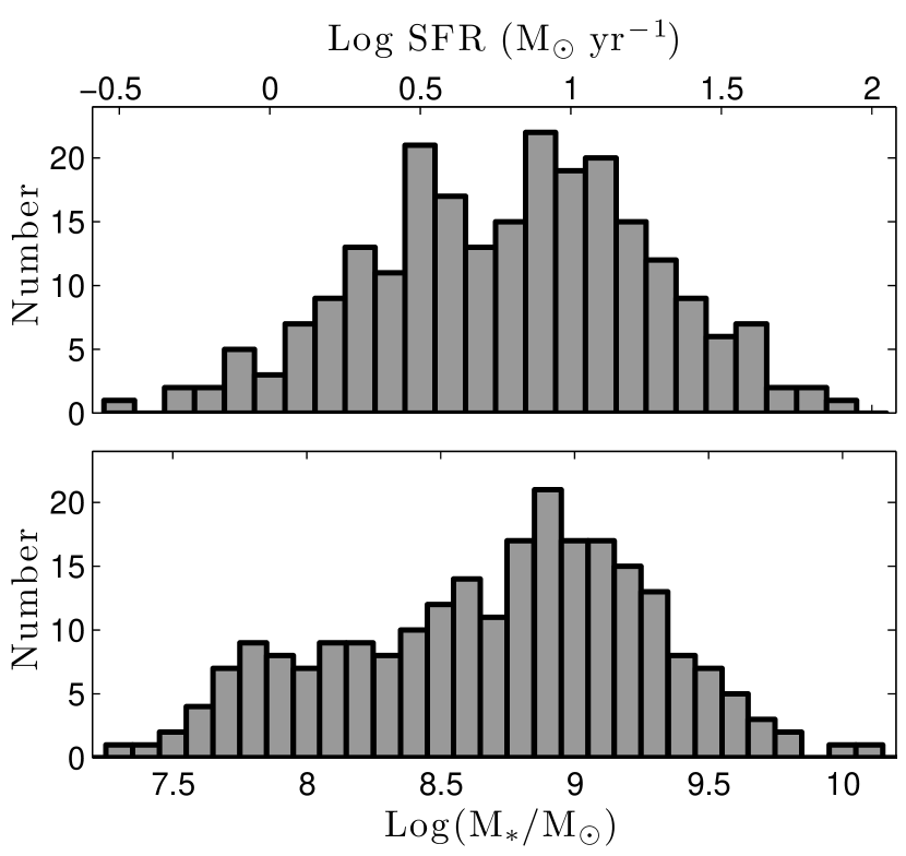
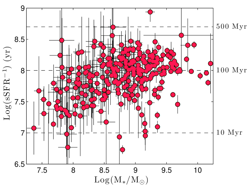
Figure 1.— Left: The stellar mass and dust-corrected UV-based SFR distributions of the 239 galaxies in our HST WFC3 IR-grism selected sample. The data span three orders of magnitude in stellar mass, and two orders of magnitude in SFR, and include objects that are generally smaller and fainter than galaxies selected via their continuum colors. Right: The mass-specific star formation rates of the galaxies as a function of their stellar mass. The error bars reflect only the statistical uncertainties associated with our measurements; the systematic offsets associated with parameters such as the assumed IMF and SFR calibration are not shown. For galaxies with a constant star formation rate, the sSFR is simply the inverse of the age, which is indicated via the right-hand labels of the figure. The data indicate that most of our galaxies have likely been forming stars for at least $\sim 100$ Myr. The observed correlation betwen sSFR and stellar mass may be affected by the SFR limit of the grism survey. This selection effect is described in more detail in Zeimann et al. (2014, 2015).

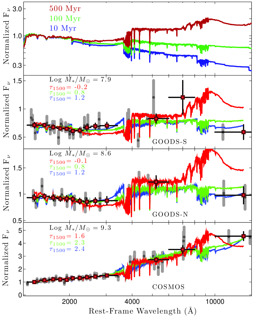
Figure 2.— The top panel shows 2007 versions of Bruzual & Charlot (2003) SEDs for populations which have been forming stars at a constant rate for 10, 100, and 500 Myr. The data have been arbitrarily normalized at 1500 Å. There is little difference between the populations in the UV; it is only in the optical and near IR where population age becomes important. The bottom three panels display three typical rest-frame SEDs from our emission-line galaxy sample. The gray bars are the de-redshifted observed filters, the red squares are the “artificial” filters with error bars illustrating the bin size, and the three colored lines correspond to best-fit, dust-attenuated model spectral energy distributions (same colors as the top plot). The attenuation curves for the best-fit models are given in Table 1, and in each panel the best-fit ${\tau}_{\rm 1500}$ value is reported. The negative ${\tau}_{\rm 1500}$ values associated with the 500 Myr SED fits for the two lower mass systems illustrate that the assumed population is too old, resulting in unphysical attenuation laws. This may be due to the treatment of asymptotic giant branch stars and is discussed in § 5.1.

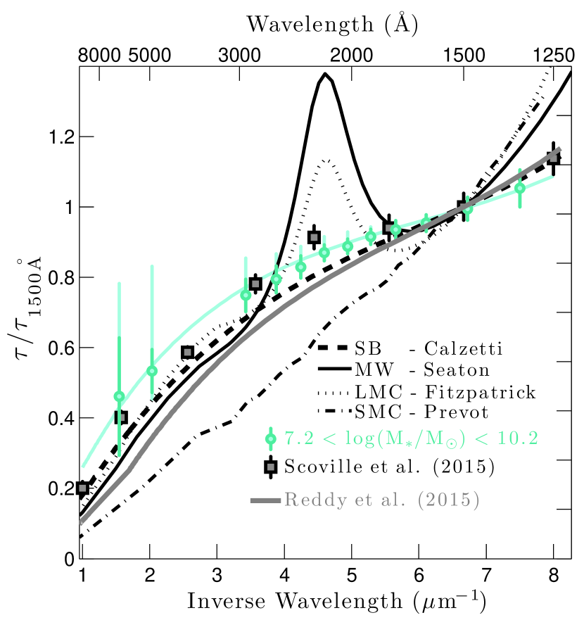
Figure 3.— Dust attenuation and extinction curves for the Milky Way (Seaton, 1979), Magellanic Clouds (Prevot et al., 1984; Fitzpatrick, 1986), the local star-bursting galaxies of Calzetti et al. (2000), the more massive $1.5<z<4$ systems of Scoville et al. (2015) and Reddy et al. (2015), and our sample of rest-frame optical emission-line galaxies. The dark blue error bars on our data indicate the statistical uncertainties for the dust attenuation curve, under the assumption of a 100 Myr constant star-forming stellar population. The light blue error bars show the extent of the systematic errors if we were to instead use our extreme models for 10 Myr and 500 Myr stellar populations. The blue solid curve indicates the Calzetti et al. (2000) attenuation law, perturbed by our best-fit values of $\delta=0.18\pm 0.05$ and $E_{b}=0.04\pm 0.27$.

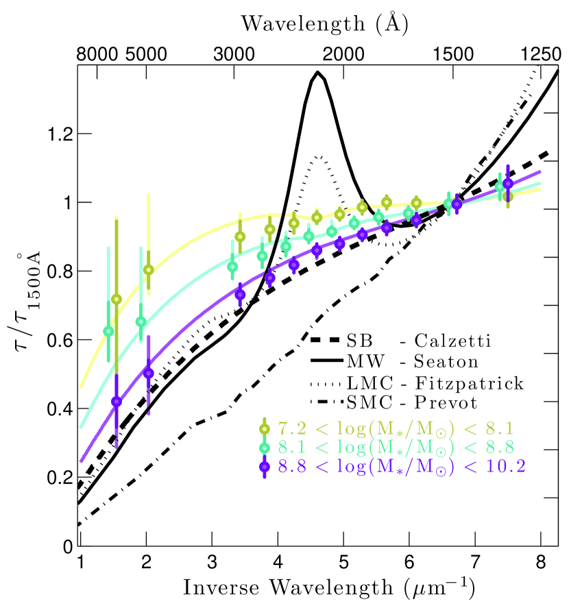
Figure 4.— Dust attenuation curves for our sample of HST WFC3 IR-grism selected galaxies split into three stellar mass bins, as well as the curves for the Milky Way (Seaton, 1979), Magellanic Clouds (Prevot et al., 1984; Fitzpatrick, 1986), and for the local star-bursting galaxies of Calzetti et al. (2000). The dark color error bars indicate the statistical uncertainties for the dust attenuation curve, under the assumption of a 100 Myr constant star-forming stellar population; the light color error bars show the extent of the systematic errors if we were to instead use our extreme models for 10 Myr and 500 Myr stellar populations. The colored curves display the Calzetti et al. (2000) attenuation law perturbed by our best-fit values for $\delta$ and $E_{b}$. The three mass bins clearly have different attenuation laws, with a shallower curve associated with least massive systems.

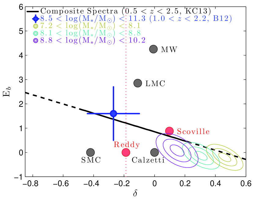
Figure 5.— Measurements of the dust attenuation law parameters as a function of galaxy stellar mass for $z\sim 2$ systems. The variable $\delta$ reflects the UV slope of the reddening curve; $E_{b}$ describes the amplitude of the 2175 Å bump. The colored ellipses represent $1$, $2$, and $3\,\sigma$ uncertainties for the three mass bins. By definition, a Calzetti et al. (2000) law has $E_{b}=\delta=0$. The trend in our measurements and those of Buat et al. (2012) agree qualitatively with that found by Kriek & Conroy (2013). In all cases, the Calzetti et al. (2000) curve is ruled out with greater than $3\,\sigma$ confidence. Also shown are the results from Scoville et al. (2015) and Reddy et al. (2015), which include galaxies that are more massive, on average, than those studied in this work. By construction, Reddy et al. (2015) do not fit for a bump in their dust attenuation curve, so we use a vertical dotted line to illustrate the uncertainty.

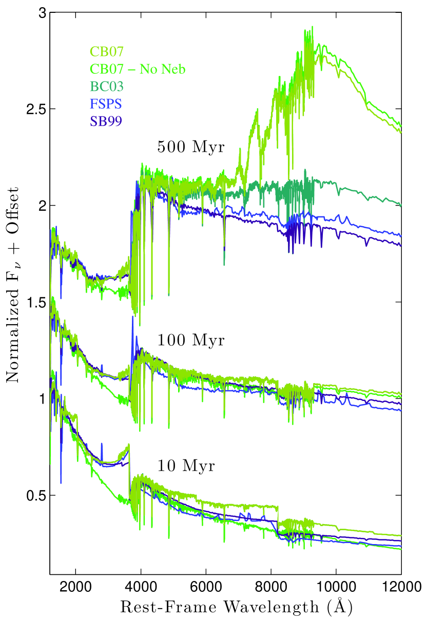
Figure 6.— A comparison of the spectral energy distributions produced by several popular population synthesis codes. The data have been arbitrarily normalized at 1500 Å. We show the SEDs create by the 2007 version of Bruzual & Charlot (2003) with and without nebular continuum emission, the original Bruzual & Charlot (2003) model, version 7.0.1 of STARBURST99, and FSPS. All of the SPS codes were set to the same stellar metallicity, $Z=0.2Z_{\odot}$ and used constant star formation histories with ages of 10, 100, and 500 Myr. There is little difference between the populations in the UV with the exception of the model without nebular continuum emission; it is only in the optical and near IR where population age and the codes’ differing assumptions become important.

References

- Acquaviva et al. (2011) Acquaviva, V., Gawiser, E., & Guaita, L. 2011, ApJ, 737, 47
- Acquaviva et al. (2012) Acquaviva, V., Vargas, C., Gawiser, E., & Guaita, L. 2012, ApJ, 751, L26
- Alexander et al. (2003) Alexander, D.M., Bauer, F.E., Brandt, W.N., et al. 2003, AJ, 126, 539
- Bouwens et al. (2009) Bouwens, R.J., Illingworth, G.D., Franx, M., et al. 2009, ApJ, 705, 936
- Brammer et al. (2012) Brammer, G.B., van Dokkum, P.G., Franx, M., et al. 2012, ApJS, 200, 13
- H. Brooks et al. (2016, in preparation) Brooks, H., Zeimann, G.R., Ciardullo, R., & Gronwall, C. 2016, in preparation
- Bruzual & Charlot (2003) Bruzual, G., & Charlot, S. 2003, MNRAS, 344, 1000
- Buat et al. (2011) Buat, V., Giovannoli, E., Heinis, S., et al. 2011, A&A, 553, A93
- Buat et al. (2012) Buat, V., Noll, S., Burgarella, D., et al. 2012, A&A, 545, AA141
- Burgarella et al. (2005) Burgarella, D., Buat, V., & Iglesias-Páramo, J. 2005, MNRAS, 360, 1413
- Calzetti et al. (1994) Calzetti, D., Kinney, A.L., & Storchi-Bergmann, T. 1994, ApJ, 429, 582
- Calzetti et al. (2000) Calzetti, D., Armus, L., Bohlin, R.C., et al. 2000, ApJ, 533, 682
- Calzetti (2001) Calzetti, D. 2001, PASP, 113, 1449
- Cardelli et al. (1989) Cardelli, J.A., Clayton, G.C., & Mathis, J.S. 1989, ApJ, 345, 245
- Charlot & Fall (2000) Charlot, S., & Fall, S.M. 2000, ApJ, 539, 718
- Ciardullo et al. (2014) Ciardullo, R., Zeimann, G.R., Gronwall, C., et al. 2014, ApJ, 796, 64
- Colbert et al. (2013) Colbert, J.W., Teplitz, H., Atek, H., et al. 2013, ApJ, 779, 34
- Coleman et al. (1980) Coleman, G. D., Wu, C.-C., & Weedman, D. W. 1980, ApJS, 43, 393
- Conroy et al. (2009) Conroy, C., Gunn, J. E., & White, M. 2009, ApJ, 699, 486
- Conroy et al. (2010) Conroy, C., Schiminovich, D., & Blanton, M.R. 2010, ApJ, 718, 184
- Conroy & Gunn (2010) Conroy, C., & Gunn, J. E. 2010, ApJ, 712, 833
- Conroy (2013) Conroy, C. 2013, ARA&A, 51, 393
- da Silva et al. (2012) da Silva, R.L., Fumagalli, M., & Krumholz, M. 2012, ApJ, 745, 145
- Draine et al. (2007) Draine, B.T., Dale, D.A., Bendo, G., et al. 2007, ApJ, 663, 866
- Draine (2011) Draine, B.T. 2011, EAS Publications Series, 46, 29
- Elvis et al. (2009) Elvis, M., Civano, F., Vignali, C., et al. 2009, ApJS, 184, 158
- Finkelstein et al. (2015) Finkelstein, S.L., Ryan, R.E., Jr., Papovich, C., et al. 2015, submitted to ApJ, 810, 71
- Fitzpatrick (1986) Fitzpatrick, E. L. 1986, AJ, 92, 1068
- Fruchter & Hook (2002) Fruchter, A.S., & Hook, R.N. 2002, PASP, 114, 144
- Garn & Best (2010) Garn, T., & Best, P.N. 2010, MNRAS, 409, 421
- Grasshorn Gebhardt et al. (2015) Grasshorn Gebhardt, H.S., Zeimann, G.R., Ciardullo, R., & Gronwall, C. 2015, submitted to ApJ
- Giavalisco et al. (2004) Giavalisco, M., Ferguson, H.C., Koekemoer, A.M., et al. 2004, ApJ, 600, L93
- Granato et al. (2000) Granato, G.L., Lacey, C.G., Silva, L., et al. 2000, ApJ, 542, 710
- Hagen et al. (2015) Hagen, A., Zeimann, G.R., Behrens, C., et al. 2015, submitted to ApJ
- Hill et al. (2008) Hill, G. J., Gebhardt, K., Komatsu, E., et al. 2008, in ASP Conf. Ser. 399, Panoramic Views of Galaxy Formation and Evolution, ed. T. Kodama, T. Yamada, & K. Aoki (San Francisco: Astronomical Society of the Pacific), 115
- Hinshaw et al. (2013) Hinshaw, G., Larson, D., Komatsu, E., et al. 2013, ApJS, 208, 19
- Hopkins et al. (2014) Hopkins, P.F., Kereš, D., Oñorbe, J., et al. 2014, MNRAS, 445, 581
- Izotov et al. (2011) Izotov, Y. I., Guseva, N. G., & Thuan, T. X. 2011, ApJ, 728, 161
- Kennicutt et al. (2003) Kennicutt, R.C., Jr., Armus, L., Bendo, G., et al. 2003, PASP, 115, 928
- Kennicutt & Evans (2012) Kennicutt, R.C., & Evans, N.J. 2012, ARA&A, 50, 531
- Koornneef & Code (1981) Koornneef, J., & Code, A.D. 1981, ApJ, 247, 860
- Kriek & Conroy (2013) Kriek, M., & Conroy, C. 2013, ApJ, 775, L16
- Kroupa (2001) Kroupa, P. 2001, MNRAS, 322, 231
- Lada & Lada (2003) Lada, C.J., & Lada, E.A. 2003, ARA&A, 41, 57
- Leitherer et al. (1999) Leitherer, C., Schaerer, D., Goldader, J.D., et al. 1999, ApJS, 123, 3
- Leitherer et al. (2010) Leitherer, C., Ortiz Otálvaro, P. A., Bresolin, F., et al. 2010, ApJS, 189, 309
- Leitherer et al. (2014) Leitherer, C., Ekström, S., Meynet, G., et al. 2014, ApJS, 212, 14
- Madau (1995) Madau, P. 1995, ApJ, 441, 18
- McLean et al. (2012) McLean, I.S., Steidel, C.C., Epps, H.W., et al. 2012, Proc. SPIE, 8446
- Noll et al. (2009) Noll, S., Pierini, D., Cimatti, A., et al. 2009, A&A, 499, 69
- Peng et al. (2010) Peng, Y.-j., Lilly, S.J., Kovač, K., et al. 2010, ApJ, 721, 193
- Penner et al. (2015) Penner, K., Dickinson, M., Weiner, B., et al. 2015, arXiv:1507.00728
- Prevot et al. (1984) Prevot, M.L., Lequeux, J., Prevot, L., Maurice, E., & Rocca-Volmerange, B. 1984, A&A, 132, 389
- Reddy et al. (2012) Reddy, N. A., Pettini, M., Steidel, C. C., et al. 2012, ApJ, 754, 25
- Reddy et al. (2015) Reddy, N.A., Kriek, M., Shapley, A.E., et al. 2015, ApJ, 806, 259
- Salpeter (1955) Salpeter, E.E. 1955, ApJ, 121, 161
- Scoville et al. (2007) Scoville, N., Aussel, H., Brusa, M., et al. 2007, ApJS, 172, 1
- Scoville et al. (2015) Scoville, N., Faisst, A., Capak, P., et al. 2015, ApJ, 800, 108
- Seaton (1979) Seaton, M. J. 1979, MNRAS, 187, 73P
- Silva et al. (1998) Silva, L., Granato, G.L., Bressan, A., & Danese, L. 1998, ApJ, 509, 103
- Skelton et al. (2014) Skelton, R.E., Whitaker, K.E., Momcheva, I.G., et al. 2014, ApJS, 214, 24
- Stecher (1965) Stecher, T.P. 1965, ApJ, 142, 1683
- Tereno et al. (2015) Tereno, I., Carvalho, C.S., Dinis, J., et al. 2015, in I.A.U. Symp 306, Statistical Challenges in 21st Century Cosmology, ed. A.F. Heavens, J.-L. Strack, & A. Krone-Martins, (Cambridge: Cambridge University Press), 379
- Tielens (2008) Tielens, A.G.G.M. 2008, ARA&A, 46, 289
- Tremonti et al. (2004) Tremonti, C.A., Heckman, T.M., Kauffmann, G., et al. 2004, ApJ, 613, 898
- Vázquez & Leitherer (2005) Vázquez, G.A., & Leitherer, C. 2005, ApJ, 621, 695
- Weiner et al. (2014) Weiner, B.J., & AGHAST Team 2014, BAAS, 223, #227.07
- Xue et al. (2011) Xue, Y.Q., Luo, B., Brandt, W.N., et al. 2011, ApJS, 195, 10
- Zeimann et al. (2014) Zeimann, G.R., Ciardullo, R., Gebhardt, H., & Gronwall, C. 2014, ApJ, 790, 113
- Zeimann et al. (2015) Zeimann, G.R., Ciardullo, R., Gebhardt, H., et al. 2015, ApJ, 798, 29