A Discontinuous Galerkin method with a modified penalty flux for the propagation and scattering of acousto-elastic waves

We develop an approach for simulating acousto-elastic wave phenomena, including scattering from fluid-solid boundaries, where the solid is allowed to be anisotropic, with the Discontinuous Galerkin method. We use a coupled first-order elastic strain-velocity, acoustic velocity-pressure formulation, and append penalty terms based on interior boundary continuity conditions to the numerical (central) flux so that the consistency condition holds for the discretized Discontinuous Galerkin weak formulation. We incorporate the fluid-solid boundaries through these penalty terms and obtain a stable algorithm. Our approach avoids the diagonalization into polarized wave constituents such as in the approach based on solving elementwise Riemann problems.

1 Introduction

The accurate computation of waves in realistic three-dimensional Earth models represents an ongoing challenge in local, regional, and global seismology. Here, we focus on simulating coupled acousto-elastic wave phenomena including scattering from fluid-solid boundaries, where the solid is allowed to be anisotropic, with the Discontinuous Galerkin method. Of particular interest are applications in geophysics, namely, marine seismic exploration and global Earth inverse problems using earthquake-generated seismic waves as the probing field. In the first application, we are concerned with the presence of the ocean bottom and in the second one with the core-mantle-boundary (CMB) and inner-core-boundary (ICB). Our formulation closely follows the analysis of existence of (weak) solutions of hyperbolic first-order systems of equations by [Blazek et al.(2013)Blazek, Stolk, & Symes]. We use an unstructured tetrahedral mesh with local refinement to accommodate highly heterogeneous media and complex geometries, which is also an underlying motivation for employing the Discontinuous Galerkin method from a computational point of view.

In the past three decades, a wide variety of numerical techniques has been employed in the development of computational methods for simulating seismic waves. The most widely used one is based on the finite difference method [e.g., [Madariaga(1976)] and [Virieux(1986)]]. This method has been applied to computing the wavefield in three-dimensional local and regional models [e.g., [Graves(1996)] and [Ohminato & Chouet(1997)]]. The use of optimal or compact finite-difference operators has provided a certain improvement [e.g., [Zingg et al.(1996)Zingg, Lomax, & Jurgens] and [Zingg(2000)]]. Methods that resort to spectral and pseudospectral techniques based on global gridding of the model have also been used both in regional [e.g., [Carcione(1994)]] and global [e.g., [Tessmer et al.(1992)Tessmer, Kessler, Kosloff, & Behle] and [Igel(1999)]] seismic wave propagation and scattering problems. However, because of the use of global basis functions (polynomial: Chebyshev or Legendre, or harmonic: Fourier), these techniques are limited to coefficients which are (piecewise) sufficiently smooth. The finite difference method suffers from a limited accuracy in the presence of a free surface or surface discontinuities with topography within the model [e.g., [Robertsson(1996)] and [Symes & Vdovina(2009)]]. A procedure for the stable imposition of free-surface boundary conditions for a second-order formulation can be found in [Appelö & Petersson(2009)]. Another approach, belonging to a broader family of interface methods, handles both free surfaces [e.g., [Lombard et al.(2008)Lombard, Piraux, Gélis, & Virieux]] and fluid-solid interfaces [e.g., [Lombard & Piraux(2004)]] in such a way, conjectured by the authors, that enables higher-order accuracy to be obtained. [Kozdon et al.(2013)Kozdon, Dunham, & Nordstr枚m] use summation-by-parts finite difference operators along with a weak enforcement of boundary conditions to develop a multi-block finite difference scheme which achieves higher-order accuracy for complex geometries.

A key development in the computation of seismic waves has been based on the spectral element method (SEM) [[Komatitsch & Tromp(2002)]]. In its original formulation, in terms of displacement [[Komatitsch & Vilotte(1998)]], continuity of displacement and velocity is enforced everywhere within the model. In the case of a boundary between an inviscid fluid and a solid, however, the kinematic boundary condition is perfect slip; therefore, only the normal component of velocity is continuous across such a boundary, and thus this formulation is not applicable. Some classical finite-element methods (FEMs) alternatively introduce coupling conditions on fluid-solid interfaces between displacement in the solid and pressure in the fluid [e.g. [Zienkiewicz & Bettess(1978), Bermúdez et al.(1999)Bermúdez, Hervella-Nieto, & Rodrıguez]].

The FEM and SEM are commonly (but not exclusively) based on the second-order form of the system of equations describing acousto-elastic waves. In this case, the acousto-elastic interaction is effected by coupling the respective wave equations through appropriate interface conditions. To resolve the coupling, a predictor-multicorrector iteration at each time step has been used [[Komatitsch et al.(2000)Komatitsch, Barnes, & Tromp], [Chaljub et al.(2003)Chaljub, Capdeville, & Vilotte]]. A computationally more efficient time stepping method for global seismic wave propagation accommodating the effects of fluid-solid boundaries, as well as transverse isotropy with a radial symmetry axis and radial models of attenuation, was proposed in [Komatitsch et al.(2005)Komatitsch, Tsuboi, & Tromp]. It uses a velocity potential formulation and a second-order accurate Newmark time integration, in which a time step is first performed in the acoustic fluid and then in the elastic solid using interface values based on the fluid solution. Currently the SEM is used in a variety of implementations in global and regional seismic simulation, with the effects of variations in elastic parameters, density, ellipticity, topography and bathymetry, fluid-solid interfaces, anisotropy, and self-gravitation included [e.g. [Carrington et al.(2008)Carrington, Komatitsch, Laurenzano, Tikir, Michéa, Le Goff, Snavely, & Tromp]].

In contrast to classical finite element discretizations, the Discontinous Galerkin (DG) method imposes continuity of approximate solutions between elements only weakly through a numerical flux. The Discontinuous Galerkin method has been employed for solving second-order wave equations in both the acoustic and elastodynamic settings [e.g. [Rivière & Wheeler(2000)], [Grote et al.(2006)Grote, Schneebeli, & Schötzau], [Chung & Engquist(2006)] and [De Basabe et al.(2008)De Basabe, Sen, & Wheeler]]. [Etienne et al.(2010)Etienne, Chaljub, Virieux, & Glinsky] employ a central numerical flux in a DG scheme combined with a leap-frog time integration for the velocity-stress elastic-wave formulation. [Dumbser & Käser(2006), Käser & Dumbser(2008)] developed a non-conservative formulation with an upwind numerical flux using only the material properties from the side of the interface that is opposite to the outer normal direction. [Wilcox et al.(2010)Wilcox, Stadler, Burstedde, & Ghattas] derived an upwind numerical flux by solving the exact Riemann problem on interior boundaries of each element with material discontinuities based on a velocity-strain formulation of the coupled acousto-elastic equations.

In this work, we essentially extend the upwind flux, given by [Warburton(2013)] for hyperbolic systems, to a penalty flux based on the boundary continuity condition for general fluid-solid interfaces. The novelties of our approach are the following: we

1. use a coupled first-order elastic strain-velocity, acoustic velocity-pressure formulation,

2. obtain a self-consistent Discontinuous Galerkin weak formulation without diagonalization into polarized wave constituents,

3. append penalty terms, derived from interior boundary continuity conditions, with an appropriate weight to the numerical (central) flux so that the consistency condition holds for the discretized Discontinuous Galerkin weak formulation,

4. incorporate fluid-solid boundaries through the mentioned penalty terms.

We note that the DG method is naturally adapted to well-posedness, in the sense that it makes use of coercivity of the operator defining the part of the system containing the spatial derivatives separately in the solid and fluid regions.

2 The system of equations describing acousto-elastic waves

We consider a bounded domain $\Omega\subset\mathbb{R}^{3}$ which is divided into solid and fluid regions, ${\Omega_{\mathrm{S}}}$ and ${\Omega_{\mathrm{F}}}$, respectively. The interior boundaries include solid-solid interface ${\Sigma_{{\scriptscriptstyle\mathrm{SS}}}}$, fluid-fluid interface ${\Sigma_{{\scriptscriptstyle\mathrm{FF}}}}$, and fluid-solid interface ${\Sigma_{{\scriptscriptstyle\mathrm{FS}}}}$, ${\Sigma_{{\scriptscriptstyle\mathrm{SF}}}}$ (where we distinguish whether the fluid or solid is on a particular side). We present the weak form of the coupled acousto-elastic system of equations.

Hooke’s law in an elastodynamical system is expressed by relating stress, $S_{ij}$, and strain, $E_{kl}$. Assuming small deformations gives a linear relationship, that is, $S_{ij}=c_{ijkl}E_{kl}$, where $c_{ijkl}$ is the stiffness tensor. Through the relevant symmetries, this tensor only contains 21 independent components. We use the Voigt notation which simplifies the writing of tensors while introducing $\textbf{\em S}=(S_{11},S_{22},S_{33},S_{23},S_{12},S_{13})^{T}$ and $\textbf{\em E}=(E_{11},E_{22},E_{33},E_{23},E_{12},E_{13})^{T}$. In this notation the stiffness tensor takes the form of a 6 by 6 matrix, C, defined by,

$$\textbf{\em S}=\textbf{\em C}\textbf{\em E},\quad\textbf{\em C}=\begin{bmatrix}C_{11}&C_{12}&C_{13}&2C_{14}&2C_{15}&2C_{16}\\[-2.84526pt] C_{12}&C_{22}&C_{13}&2C_{24}&2C_{25}&2C_{26}\\[-2.84526pt] C_{13}&C_{23}&C_{33}&2C_{34}&2C_{35}&2C_{36}\\[-2.84526pt] C_{14}&C_{24}&C_{34}&2C_{44}&2C_{45}&2C_{46}\\[-2.84526pt] C_{15}&C_{25}&C_{35}&2C_{45}&2C_{55}&2C_{56}\\[-2.84526pt] C_{16}&C_{26}&C_{36}&2C_{46}&2C_{56}&2C_{66}\end{bmatrix}.$$ (1)

The isotropic case is obtained by setting all of the $C_{ij}$ components to zero except for $C_{11}=\lambda+2\mu$, $C_{12}=C_{13}=C_{23}=\lambda$, $C_{44}=\mu$, $C_{55}=\mu$, and $C_{66}=\mu$; $(\lambda,\mu)$ are the Lamé parameters. Furthermore, $\rho$ denotes the density. The anisotropic elastodynamical equations are written in terms of the strain, E, and the particle velocity, v,

$$\frac{\partial\textbf{\em E}}{\partial t}=\tfrac{1}{2}\left(\nabla\textbf{\em v}+\nabla\textbf{\em v}^{T}\right),\quad\rho\,\frac{\partial\textbf{\em v}}{\partial t}=\nabla\cdot(\textbf{\em C}\textbf{\em E})+\textbf{\em f}$$ (2)

in ${\Omega_{\mathrm{S}}}$. In fluid regions, ${\Omega_{\mathrm{F}}}$, we use the pressure-velocity formulation,

$$\frac{\partial\widetilde{E}}{\partial t}=\nabla\cdot\widetilde{\textbf{\em v}}-\frac{\widetilde{f}}{\widetilde{\lambda}},\quad\widetilde{\rho}\,\frac{\partial\widetilde{\textbf{\em v}}}{\partial t}=\nabla(\widetilde{\lambda}\widetilde{E}).$$ (3)

Here, $\widetilde{P}=-\widetilde{\lambda}\widetilde{E}$ is the pressure, while we use $\ \widetilde{}\$ to distinguish acoustic field quantities and material parameters from the elastic ones. In the above, $\widetilde{f}$ denotes a volume source density of injection and f denotes a volume source density of force.

The solid-solid, fluid-solid and fluid-fluid boundary conditions are given by

$$\textbf{\em v}^{+}-\textbf{\em v}^{-}=0 \textbf{\em n}\cdot{(\textbf{\em C}\textbf{\em E}\,)}^{+}-\textbf{\em n}\cdot{(\textbf{\em C}\textbf{\em E}\,)}^{-}=0 \quad\quad\text{ on }{\Sigma_{{\scriptscriptstyle\mathrm{SS}}}},$$ and (4a)

$$\textbf{\em n}\cdot(\textbf{\em v}^{\pm}-\widetilde{\textbf{\em v}}^{\mp})=0 \textbf{\em n}\cdot{(\textbf{\em C}\textbf{\em E}\,)}^{\pm}-(\widetilde{\lambda}\widetilde{E})^{\mp}\textbf{\em n}=0 \quad\quad\text{ on }{\Sigma_{{\scriptscriptstyle\mathrm{SF}}}}\mbox{ and }{\Sigma_{{\scriptscriptstyle\mathrm{FS}}}},$$ and (4b)

$$\textbf{\em n}\cdot(\widetilde{\textbf{\em v}}^{+}-\widetilde{\textbf{\em v}}^{-})=0 (\widetilde{\lambda}\widetilde{E})^{+}-(\widetilde{\lambda}\widetilde{E})^{-}=0 \quad\quad\mbox{ on }{\Sigma_{{\scriptscriptstyle\mathrm{FF}}}}.$$ and (4c)

The $\pm$ convention is determined by the direction of the interface normal, n. The outer normal vector points in the direction of the “$+$” side of the interface.

We introduce test functions (tensors) $\textbf{\em H},\textbf{\em w}$ in the solid regions and $\widetilde{\textbf{\em w}},\widetilde{H}$ in the fluid regions, which are assumed to be contained in the same spaces and satisfy the same boundary conditions as $\textbf{\em E},\textbf{\em v},\widetilde{\textbf{\em v}}$ and $\widetilde{E}$. Using (2) and (3), we find that

$$\int_{{\Omega_{\mathrm{S}}}}\frac{\partial\textbf{\em E}}{\partial t}:(\textbf{\em C}\textbf{\em H}\,)\,\mathrm{d}\Omega =\int_{{\Omega_{\mathrm{S}}}}\tfrac{1}{2}(\nabla\textbf{\em v}+\nabla\textbf{\em v}^{T}):(\textbf{\em C}\textbf{\em H}\,)\,\mathrm{d}\Omega,$$ (5a)

$$\int_{{\Omega_{\mathrm{S}}}}\rho\,\frac{\partial\textbf{\em v}}{\partial t}\cdot\textbf{\em w}\,\mathrm{d}\Omega =\int_{{\Omega_{\mathrm{S}}}}(\nabla\cdot(\textbf{\em C}\textbf{\em E}\,))\cdot\textbf{\em w}\,\mathrm{d}\Omega+\int_{{\Omega_{\mathrm{S}}}}\textbf{\em f}\cdot\textbf{\em w}\,\mathrm{d}\Omega,$$ (5b)

$$\int_{{\Omega_{\mathrm{F}}}}\frac{\partial\widetilde{E}}{\partial t}\widetilde{\lambda}\,\widetilde{H}\,\mathrm{d}\Omega =\int_{{\Omega_{\mathrm{F}}}}(\nabla\cdot\widetilde{\textbf{\em v}})\widetilde{\lambda}\,\widetilde{H}\,\mathrm{d}\Omega-\int_{{\Omega_{\mathrm{F}}}}\widetilde{f}\,\widetilde{H}\,\mathrm{d}\Omega,$$ (5c)

$$\int_{{\Omega_{\mathrm{F}}}}\widetilde{\rho}\,\frac{\partial\widetilde{\textbf{\em v}}}{\partial t}\cdot\widetilde{\textbf{\em w}}\,\mathrm{d}\Omega =\int_{{\Omega_{\mathrm{F}}}}\nabla(\widetilde{\lambda}\widetilde{E})\cdot\widetilde{\textbf{\em w}}\,\mathrm{d}\Omega.$$ (5d)

Assuming an outer traction-free boundary condition in (5b) and an outer pressure-free boundary condition in (5c), and applying an integration by parts, we obtain

$$\int_{{\Omega_{\mathrm{S}}}}\rho\,\frac{\partial\textbf{\em v}}{\partial t}\cdot\textbf{\em w}\,\mathrm{d}\Omega= -\int_{{\Omega_{\mathrm{S}}}}{(\textbf{\em C}\textbf{\em E}\,)}:\nabla\textbf{\em w}\,\mathrm{d}\Omega+\int_{{\Sigma_{{\scriptscriptstyle\mathrm{FS}}}}}(\textbf{\em n}\cdot{(\textbf{\em C}\textbf{\em E}\,)}^{-})\cdot\textbf{\em w}^{-}\,\mathrm{d}\Sigma+\int_{{\Omega_{\mathrm{S}}}}\textbf{\em f}\cdot\textbf{\em w}\,\mathrm{d}\Omega,$$ (6a)

$$\int_{{\Omega_{\mathrm{F}}}}\frac{\partial\widetilde{E}}{\partial t}\widetilde{\lambda}\,\widetilde{H}\,\mathrm{d}\Omega= -\int_{{\Omega_{\mathrm{F}}}}\widetilde{\textbf{\em v}}\cdot\nabla(\widetilde{\lambda}\widetilde{H})\,\mathrm{d}\Omega+\int_{{\Sigma_{{\scriptscriptstyle\mathrm{FS}}}}}(\textbf{\em n}\cdot\widetilde{\textbf{\em v}}^{-})(\widetilde{\lambda}\widetilde{H})^{-}\,\mathrm{d}\Sigma-\int_{{\Omega_{\mathrm{F}}}}\widetilde{f}\,\widetilde{H}\,\mathrm{d}\Omega.$$ (6b)

We use the fluid-solid boundary conditions (4b), replacing the fluid-solid surface integrals in (6a) and (6b) by taking the average of both sides consistent with a central flux scheme, and obtain

$$\int_{{\Omega_{\mathrm{S}}}}\rho\,\frac{\partial\textbf{\em v}}{\partial t}\cdot\textbf{\em w}\,\mathrm{d}\Omega =-\int_{{\Omega_{\mathrm{S}}}}{(\textbf{\em C}\textbf{\em E}\,)}:\nabla\textbf{\em w}\,\mathrm{d}\Omega$$

$$+\int_{{\Sigma_{{\scriptscriptstyle\mathrm{FS}}}}}\tfrac{1}{2}((\widetilde{\lambda}\widetilde{E})^{+}\textbf{\em n}+\textbf{\em n}\cdot{(\textbf{\em C}\textbf{\em E}\,)}^{-})\cdot\textbf{\em w}^{-}\,\mathrm{d}\Sigma+\int_{{\Omega_{\mathrm{S}}}}\textbf{\em f}\cdot\textbf{\em w}\,\mathrm{d}\Omega,$$ (7a)

$$\int_{{\Omega_{\mathrm{F}}}}\frac{\partial\widetilde{E}}{\partial t}\widetilde{\lambda}\widetilde{H}\,\mathrm{d}\Omega =-\int_{{\Omega_{\mathrm{F}}}}\widetilde{\textbf{\em v}}\cdot\nabla(\widetilde{\lambda}\widetilde{H})\,\mathrm{d}\Omega$$

$$+\int_{{\Sigma_{{\scriptscriptstyle\mathrm{FS}}}}}{\tfrac{1}{2}(\textbf{\em n}\cdot\textbf{\em v}^{-}+\textbf{\em n}\cdot\widetilde{\textbf{\em v}}^{+})}\,(\widetilde{\lambda}\widetilde{H})^{-}\,\mathrm{d}\Sigma-\int_{{\Omega_{\mathrm{F}}}}\widetilde{f}\,\widetilde{H}\,\mathrm{d}\Omega.$$ (7b)

This form of the equations is analogous to the one used in the spectral element method, see [Chaljub & Valette(2004)]. Applying an integration by parts, again, in (7), we recover the coupled strong formulation,

$$\int_{{\Omega_{\mathrm{S}}}}\rho\,\frac{\partial\textbf{\em v}}{\partial t}\cdot\textbf{\em w}\,\mathrm{d}\Omega =\int_{{\Omega_{\mathrm{S}}}}(\nabla\cdot{(\textbf{\em C}\textbf{\em E}\,)})\cdot\textbf{\em w}\,\mathrm{d}\Omega$$

$$+\int_{{\Sigma_{{\scriptscriptstyle\mathrm{FS}}}}}{\tfrac{1}{2}}((\widetilde{\lambda}\widetilde{E})^{+}\textbf{\em n}-\textbf{\em n}\cdot{(\textbf{\em C}\textbf{\em E}\,)}^{-})\cdot\textbf{\em w}^{-}\,\mathrm{d}\Sigma+\int_{{\Omega_{\mathrm{S}}}}\textbf{\em f}\cdot\textbf{\em w}\,\mathrm{d}\Omega,$$ (8a)

$$\int_{{\Omega_{\mathrm{F}}}}\frac{\partial\widetilde{E}}{\partial t}\widetilde{\lambda}\widetilde{H}\,\mathrm{d}\Omega =\int_{{\Omega_{\mathrm{F}}}}(\nabla\cdot\widetilde{\textbf{\em v}})\widetilde{\lambda}\widetilde{H}\,\mathrm{d}\Omega$$

$$+\int_{{\Sigma_{{\scriptscriptstyle\mathrm{FS}}}}}{\tfrac{1}{2}}(\textbf{\em n}\cdot(\textbf{\em v}^{+}-\widetilde{\textbf{\em v}}^{-}))\,(\widetilde{\lambda}\widetilde{H})^{-}\,\mathrm{d}\Sigma-\int_{{\Omega_{\mathrm{F}}}}\widetilde{f}\,\widetilde{H}\,\mathrm{d}\Omega.$$ (8b)

We use this system of equations together with (5a) and (5d) to develop our Discontinuous Galerkin method based approach.

3 Discontinuous Galerkin method with fluid-solid boundaries

The domain is partitioned into elements, $D^{e}$. We distinguish elements, ${D^{\mathrm{e}}_{\scriptscriptstyle\mathrm{S}}}$, in the solid regions from elements, ${D^{\mathrm{e}}_{\scriptscriptstyle\mathrm{F}}}$, in the fluid regions. Correspondingly, we distinguish fluid-fluid (${\Sigma_{{\scriptscriptstyle\mathrm{FF}}}^{\mathrm{e}}}$), solid-solid (${\Sigma_{{\scriptscriptstyle\mathrm{SS}}}^{\mathrm{e}}}$) and fluid-solid (${\Sigma_{{\scriptscriptstyle\mathrm{FS}}}^{\mathrm{e}}},{\Sigma_{{\scriptscriptstyle\mathrm{SF}}}^{\mathrm{e}}}$) faces for each element; thus the interior boundaries are decomposed as

$$\Sigma_{\ast\,\bullet}=\cup\Sigma_{\ast\,\bullet}^{\mathrm{e}},\quad\ast,\,\bullet\in\{\mathrm{S},\mathrm{F}\},$$

and so are the elements’ boundaries: $\partial{D^{\mathrm{e}}_{\scriptscriptstyle\mathrm{S}}}={\Sigma_{{\scriptscriptstyle\mathrm{SS}}}^{\mathrm{e}}}\cup{\Sigma_{{\scriptscriptstyle\mathrm{SF}}}^{\mathrm{e}}}$ and $\partial{D^{\mathrm{e}}_{\scriptscriptstyle\mathrm{F}}}={\Sigma_{{\scriptscriptstyle\mathrm{FF}}}^{\mathrm{e}}}\cup{\Sigma_{{\scriptscriptstyle\mathrm{FS}}}^{\mathrm{e}}}$. The mesh size, $h$, is defined as the maximum radius of each tetrahedral’s inscribed sphere.

We introduce the broken polynomial space $V_{h}=\bigoplus_{{D^{\mathrm{e}}}}V_{h}^{{D^{\mathrm{e}}}}$ where the local space is defined elementwise as $V_{h}^{{D^{\mathrm{e}}}}=\mathrm{span}\{\phi_{n}({D^{\mathrm{e}}})\}_{n=1}^{N_{\mathrm{dof}}^{D^{e}}}$, with $\phi_{n}$ a set of polynomial basis further discussed in Section 3.2. The subscript “$h$” indicates the refinement of $V_{h}$ with decrease in mesh size. The semi-discrete time-domain, discontinuous Galerkin formulation using a central flux yields: Find $\textbf{\em E}_{h},\textbf{\em v}_{h},\widetilde{\textbf{\em v}}_{h},\widetilde{E}_{h}$, with each component for each one of them in $V_{h}$ such that

$$\begin{split}&\int_{{D^{\mathrm{e}}_{\scriptscriptstyle\mathrm{S}}}}\frac{\partial\textbf{\em E}_{h}}{\partial t}:(\textbf{\em C}\textbf{\em H}_{h})\,\mathrm{d}\Omega+\int_{{D^{\mathrm{e}}_{\scriptscriptstyle\mathrm{S}}}}\rho\,\frac{\partial\textbf{\em v}_{h}}{\partial t}\cdot\textbf{\em w}_{h}\,\mathrm{d}\Omega\\ &\hskip 8.5359pt-\int_{{D^{\mathrm{e}}_{\scriptscriptstyle\mathrm{S}}}}\tfrac{1}{2}(\nabla\textbf{\em v}_{h}+\nabla\textbf{\em v}_{h}^{T}):(\textbf{\em C}\textbf{\em H}_{h})\,\mathrm{d}\Omega-\int_{{D^{\mathrm{e}}_{\scriptscriptstyle\mathrm{S}}}}(\nabla\cdot(\textbf{\em C}\textbf{\em E}_{h}))\cdot\textbf{\em w}_{h}\,\mathrm{d}\Omega\\ &\hskip 8.5359pt-\int_{{\Sigma_{{\scriptscriptstyle\mathrm{SS}}}^{\mathrm{e}}}}\tfrac{1}{2}{\,[\![\textbf{\em v}_{h}\,]\!]}_{\scriptscriptstyle\mathrm{SS}}\cdot(\textbf{\em n}\cdot(\textbf{\em C}\textbf{\em H}_{h})^{-})\,\mathrm{d}\Sigma-\int_{{\Sigma_{{\scriptscriptstyle\mathrm{SF}}}^{\mathrm{e}}}}{\color[rgb]{0,0,0}\tfrac{1}{2}}{\,[\![\textbf{\em v}_{h}\,]\!]}_{\scriptscriptstyle\mathrm{SF}}\cdot(\textbf{\em n}\cdot(\textbf{\em C}\textbf{\em H}_{h})^{-})\,\mathrm{d}\Sigma\\ &\hskip 8.5359pt-\int_{{\Sigma_{{\scriptscriptstyle\mathrm{SS}}}^{\mathrm{e}}}}\tfrac{1}{2}\textbf{\em n}\cdot({\,[\![\textbf{\em C}\textbf{\em E}_{h}\,]\!]}_{\scriptscriptstyle\mathrm{SS}})\cdot\textbf{\em w}_{h}^{-}\,\mathrm{d}\Sigma-\int_{{\Sigma_{{\scriptscriptstyle\mathrm{SF}}}^{\mathrm{e}}}}{\tfrac{1}{2}}\textbf{\em n}\cdot({\,[\![\textbf{\em C}\textbf{\em E}_{h}\,]\!]}_{\scriptscriptstyle\mathrm{SF}})\cdot\textbf{\em w}_{h}^{-}\,\mathrm{d}\Sigma=\int_{{D^{\mathrm{e}}_{\scriptscriptstyle\mathrm{S}}}}\textbf{\em f}_{h}\cdot\textbf{\em w}_{h}\,\mathrm{d}\Omega,\end{split}$$ (9)

and

$$\begin{split}&\int_{{D^{\mathrm{e}}_{\scriptscriptstyle\mathrm{F}}}}\frac{\partial\widetilde{E}_{h}}{\partial t}\widetilde{\lambda}\widetilde{H}_{h}\,\mathrm{d}\Omega+\int_{{D^{\mathrm{e}}_{\scriptscriptstyle\mathrm{F}}}}\widetilde{\rho}\,\frac{\partial\widetilde{\textbf{\em v}}_{h}}{\partial t}\cdot\widetilde{\textbf{\em w}}_{h}\,\mathrm{d}\Omega\\ &\hskip 8.5359pt-\int_{{D^{\mathrm{e}}_{\scriptscriptstyle\mathrm{F}}}}(\nabla\cdot\widetilde{\textbf{\em v}}_{h})\,\widetilde{\lambda}\widetilde{H}_{h}\,\mathrm{d}\Omega-\int_{{D^{\mathrm{e}}_{\scriptscriptstyle\mathrm{F}}}}\nabla(\widetilde{\lambda}\widetilde{E}_{h})\cdot\widetilde{\textbf{\em w}}_{h}\,\mathrm{d}\Omega\\ &\hskip 8.5359pt-\int_{{\Sigma_{{\scriptscriptstyle\mathrm{FF}}}^{\mathrm{e}}}}\tfrac{1}{2}(\textbf{\em n}\cdot{\,[\![\widetilde{\textbf{\em v}}_{h}\,]\!]}_{\scriptscriptstyle\mathrm{FF}})\,(\widetilde{\lambda}\widetilde{H}_{h})^{-}\,\mathrm{d}\Sigma-\int_{{\Sigma_{{\scriptscriptstyle\mathrm{FS}}}^{\mathrm{e}}}}{\tfrac{1}{2}}(\textbf{\em n}\cdot{\,[\![\widetilde{\textbf{\em v}}_{h}\,]\!]}_{\scriptscriptstyle\mathrm{FS}})\,(\widetilde{\lambda}\widetilde{H}_{h})^{-}\,\mathrm{d}\Sigma\\ &\hskip 8.5359pt-\int_{{\Sigma_{{\scriptscriptstyle\mathrm{FF}}}^{\mathrm{e}}}}\tfrac{1}{2}{\,[\![\widetilde{\lambda}\widetilde{E}_{h}\,]\!]}_{\scriptscriptstyle\mathrm{FF}}(\textbf{\em n}\cdot\textbf{\em w}_{h}^{-})\,\mathrm{d}\Sigma-\int_{{\Sigma_{{\scriptscriptstyle\mathrm{FS}}}^{\mathrm{e}}}}{\tfrac{1}{2}}{\,[\![\widetilde{\lambda}\widetilde{E}_{h}\,]\!]}_{\scriptscriptstyle\mathrm{FS}}(\textbf{\em n}\cdot\textbf{\em w}_{h}^{-})\,\mathrm{d}\Sigma=-\int_{{D^{\mathrm{e}}_{\scriptscriptstyle\mathrm{F}}}}\widetilde{f}_{h}\,\widetilde{H}_{h}\,\mathrm{d}\Omega,\end{split}$$ (10)

hold for each element ${D^{\mathrm{e}}_{\scriptscriptstyle\mathrm{S}}}$ or ${D^{\mathrm{e}}_{\scriptscriptstyle\mathrm{F}}}$, for all test functions $\textbf{\em H}_{h},\textbf{\em w}_{h},\widetilde{\textbf{\em w}}_{h},\widetilde{H}_{h}{\in V_{h}}$. The notations $\textbf{\em f}_{h}$ and $\widetilde{f}_{h}$ indicate polynomial approximation of f and $\widetilde{f}$. Here,

$$\begin{array}[]{rl}{\,[\![\textbf{\em v}\,]\!]}_{\scriptscriptstyle\mathrm{SS}}=&\textbf{\em v}^{+}-\textbf{\em v}^{-}\\ {\,[\![\textbf{\em C}\textbf{\em E}\,]\!]}_{\scriptscriptstyle\mathrm{SS}}=&\textbf{\em n}\,(\textbf{\em n}\cdot(\textbf{\em C}\textbf{\em E})^{+}-\textbf{\em n}\cdot(\textbf{\em C}\textbf{\em E})^{-})\end{array} \quad\mbox{ on }{\Sigma_{{\scriptscriptstyle\mathrm{SS}}}^{\mathrm{e}}},$$ (11c)

$$\begin{array}[]{rl}{\,[\![\textbf{\em v}\,]\!]}_{\scriptscriptstyle\mathrm{SF}}=&(\textbf{\em n}\cdot(\widetilde{\textbf{\em v}}^{+}-\textbf{\em v}^{-}))\textbf{\em n}\\ {\,[\![\textbf{\em C}\textbf{\em E}\,]\!]}_{\scriptscriptstyle\mathrm{SF}}=&\textbf{\em n}\,((\widetilde{\lambda}\widetilde{E})^{+}\textbf{\em n}-\textbf{\em n}\cdot(\textbf{\em C}\textbf{\em E})^{-})\end{array} \quad\mbox{ on }{\Sigma_{{\scriptscriptstyle\mathrm{SF}}}^{\mathrm{e}}}$$ (11f)

in the solid regions, while

$$\begin{array}[]{rl}{\,[\![\widetilde{\textbf{\em v}}\,]\!]}_{\scriptscriptstyle\mathrm{FF}}=&(\textbf{\em n}\cdot(\widetilde{\textbf{\em v}}^{+}-\widetilde{\textbf{\em v}}^{-}))\textbf{\em n}\\ {\,[\![\widetilde{\lambda}\widetilde{E}\,]\!]}_{\scriptscriptstyle\mathrm{FF}}=&(\widetilde{\lambda}\widetilde{E})^{+}-(\widetilde{\lambda}\widetilde{E})^{-}\end{array} \quad\mbox{ on }{\Sigma_{{\scriptscriptstyle\mathrm{FF}}}^{\mathrm{e}}},$$ (12c)

$$\begin{array}[]{rl}{\,[\![\widetilde{\textbf{\em v}}\,]\!]}_{\scriptscriptstyle\mathrm{FS}}=&(\textbf{\em n}\cdot(\textbf{\em v}^{+}-\widetilde{\textbf{\em v}}^{-}))\textbf{\em n}\\ {\,[\![\widetilde{\lambda}\widetilde{E}\,]\!]}_{\scriptscriptstyle\mathrm{FS}}=&\textbf{\em n}\cdot(\textbf{\em C}\textbf{\em E})^{+}\cdot\textbf{\em n}-(\widetilde{\lambda}\widetilde{E})^{-}\end{array} \quad\mbox{ on }{\Sigma_{{\scriptscriptstyle\mathrm{FS}}}^{\mathrm{e}}}$$ (12f)

in the fluid regions, using interior boundary continuity conditions. A similar formulation for Maxwell’s equations, using the central flux, can be found in [Hesthaven & Warburton(2007), Chapter 10, Page 434].

3.1 Energy function of central flux

We consider a time-dependent energy function comprising both the solid and fluid regions, ${\mathcal{E}}_{h}={\mathcal{E}}_{\mathrm{S},h}+{\mathcal{E}}_{\mathrm{F},h}$, with

$$\begin{split}{\mathcal{E}}_{\mathrm{S},h}&=\tfrac{1}{2}{\sum_{\mathrm{e}}}\int_{D^{\mathrm{e}}_{\scriptscriptstyle\mathrm{S}}}(\textbf{\em E}_{h}:(\textbf{\em C}\textbf{\em E}_{h})+\rho\,\textbf{\em v}_{h}\cdot\textbf{\em v}_{h})\,\mathrm{d}\Omega,\\ {\mathcal{E}}_{\mathrm{F},h}&=\tfrac{1}{2}{\sum_{\mathrm{e}}}\int_{D^{\mathrm{e}}_{\scriptscriptstyle\mathrm{F}}}\left(\widetilde{\lambda}\widetilde{E}_{h}^{2}+\widetilde{\rho}\,\widetilde{\textbf{\em v}}_{h}\cdot\widetilde{\textbf{\em v}}_{h}\right)\,\mathrm{d}\Omega.\end{split}$$ (13)

The functions in (13) define a norm both in the solid and in the fluid regions. Taking the time derivative and noting that C is symmetric, we have

$$\frac{\,\mathrm{d}{\mathcal{E}}_{\mathrm{S},h}}{\,\mathrm{d}t} ={\sum_{\mathrm{e}}}\int_{D^{\mathrm{e}}_{\scriptscriptstyle\mathrm{S}}}\left(\frac{\partial\textbf{\em E}_{h}}{\partial t}:(\textbf{\em C}\textbf{\em E}_{h})+\rho\,\frac{\partial\textbf{\em v}_{h}}{\partial t}\cdot\textbf{\em v}_{h}\right)\,\mathrm{d}\Omega,$$ (14)

$$\frac{\,\mathrm{d}{\mathcal{E}}_{\mathrm{F},h}}{\,\mathrm{d}t} ={\sum_{\mathrm{e}}}\int_{D^{\mathrm{e}}_{\scriptscriptstyle\mathrm{F}}}\left(\frac{\partial\widetilde{E}_{h}}{\partial t}\widetilde{\lambda}\widetilde{E}_{h}+\widetilde{\rho}\,\frac{\partial\widetilde{\textbf{\em v}}_{h}}{\partial t}\cdot\widetilde{\textbf{\em v}}_{h}\right)\,\mathrm{d}\Omega.$$ (15)

Starting from (9) and (10) and carrying out the summation over all the elements yields

$$\frac{\,\mathrm{d}{\mathcal{E}}_{h}}{\,\mathrm{d}t}={\sum_{\mathrm{e}}}\int_{D^{\mathrm{e}}_{\scriptscriptstyle\mathrm{S}}}\textbf{\em f}_{h}\cdot\textbf{\em v}_{h}\,\mathrm{d}\Omega-{\sum_{\mathrm{e}}}\int_{D^{\mathrm{e}}_{\scriptscriptstyle\mathrm{F}}}\widetilde{f}_{h}\,\widetilde{E}_{h}\,\mathrm{d}\Omega.$$ (16)

This property is obtained as follows:

In (9) and (10) we let $\textbf{\em H}_{h}=\textbf{\em E}_{h},\textbf{\em w}_{h}=\textbf{\em v}_{h},\widetilde{H}_{h}=\widetilde{E}_{h},\widetilde{\textbf{\em w}}_{h}=\widetilde{\textbf{\em v}}_{h}$, and obtain elementwise

$$\begin{split}&\int_{{D^{\mathrm{e}}_{\scriptscriptstyle\mathrm{S}}}}\tfrac{1}{2}(\nabla\textbf{\em v}_{h}+\nabla\textbf{\em v}_{h}^{T}):(\textbf{\em C}\textbf{\em E}_{h})\,\mathrm{d}\Omega+\int_{{D^{\mathrm{e}}_{\scriptscriptstyle\mathrm{S}}}}(\nabla\cdot(\textbf{\em C}\textbf{\em E}_{h}))\cdot\textbf{\em v}_{h}\,\mathrm{d}\Omega\\ =&\int_{{\Sigma_{{\scriptscriptstyle\mathrm{SS}}}^{\mathrm{e}}}\cup{\Sigma_{{\scriptscriptstyle\mathrm{SF}}}^{\mathrm{e}}}}\textbf{\em v}_{h}^{-}\cdot(\textbf{\em n}\cdot(\textbf{\em C}\textbf{\em E}_{h})^{-})\,\mathrm{d}\Sigma,\end{split}$$ (17)

and similarily

$$\begin{split}&\int_{{D^{\mathrm{e}}_{\scriptscriptstyle\mathrm{F}}}}(\nabla\cdot\widetilde{\textbf{\em v}}_{h})\,\widetilde{\lambda}\widetilde{E}_{h}\,\mathrm{d}\Omega+\int_{{D^{\mathrm{e}}_{\scriptscriptstyle\mathrm{F}}}}\nabla(\widetilde{\lambda}\widetilde{E}_{h})\cdot\widetilde{\textbf{\em v}}_{h}\,\mathrm{d}\Omega\\ =&\int_{{\Sigma_{{\scriptscriptstyle\mathrm{FF}}}^{\mathrm{e}}}\cup{\Sigma_{{\scriptscriptstyle\mathrm{FS}}}^{\mathrm{e}}}}\textbf{\em n}\cdot\widetilde{\textbf{\em v}}_{h}^{-}\,(\widetilde{\lambda}\widetilde{E}_{h})^{-}\,\mathrm{d}\Sigma.\end{split}$$ (18)

From (9), (11), (14) and (17),

$$\frac{\,\mathrm{d}{\mathcal{E}}_{\mathrm{S},h}}{\,\mathrm{d}t}={\sum_{\mathrm{e}}}\int_{D^{\mathrm{e}}_{\scriptscriptstyle\mathrm{S}}}\textbf{\em f}_{h}\cdot\textbf{\em v}_{h}\,\mathrm{d}\Omega$$

$$+{\sum_{\mathrm{e}}}\tfrac{1}{2}\int_{{\Sigma_{{\scriptscriptstyle\mathrm{SF}}}^{\mathrm{e}}}}\left(({\,[\![\textbf{\em v}_{h}\,]\!]}_{\scriptscriptstyle\mathrm{SF}}+\textbf{\em v}_{h}^{-})\cdot(\textbf{\em n}\cdot(\textbf{\em C}\textbf{\em E}_{h})^{-})+\textbf{\em n}\cdot({\,[\![\textbf{\em C}\textbf{\em E}_{h}\,]\!]}_{\scriptscriptstyle\mathrm{SF}}+(\textbf{\em C}\textbf{\em E}_{h})^{-})\cdot\textbf{\em v}_{h}^{-}\right)\,\mathrm{d}\Sigma \Theta_{1}$$ ()

$$+{\sum_{\mathrm{e}}}\tfrac{1}{2}\int_{{\Sigma_{{\scriptscriptstyle\mathrm{SS}}}^{\mathrm{e}}}}\left(({\,[\![\textbf{\em v}_{h}\,]\!]}_{\scriptscriptstyle\mathrm{SS}}+\textbf{\em v}_{h}^{-})\cdot(\textbf{\em n}\cdot(\textbf{\em C}\textbf{\em E}_{h})^{-})+\textbf{\em n}\cdot({\,[\![\textbf{\em C}\textbf{\em E}_{h}\,]\!]}_{\scriptscriptstyle\mathrm{SS}}+(\textbf{\em C}\textbf{\em E}_{h})^{-})\cdot\textbf{\em v}_{h}^{-}\right)\,\mathrm{d}\Sigma. \Theta_{2}$$ ()

In the above,

$$\Theta_{2}={\sum_{\mathrm{e}}}\tfrac{1}{2}\int_{{\Sigma_{{\scriptscriptstyle\mathrm{SS}}}^{\mathrm{e}}}}\left(\textbf{\em v}_{h}^{+}\cdot(\textbf{\em n}\cdot(\textbf{\em C}\textbf{\em E}_{h})^{-})+\textbf{\em n}\cdot(\textbf{\em C}\textbf{\em E}_{h})^{+}\cdot\textbf{\em v}_{h}^{-}\right)\,\mathrm{d}\Sigma=0.$$ (19)

The surface integration terms cancel out when summed from both sides of the solid-solid interfaces because of the continuity condition (4a) and the opposite outer normal directions. We are left with the contributions from solid-fluid inner faces, $\Theta_{1}$,

$$\frac{\,\mathrm{d}{\mathcal{E}}_{\mathrm{S},h}}{\,\mathrm{d}t}={\sum_{\mathrm{e}}}\tfrac{1}{2}\int_{{\Sigma_{{\scriptscriptstyle\mathrm{SF}}}^{\mathrm{e}}}}\left(\widetilde{\textbf{\em v}}_{h}^{+}\cdot(\textbf{\em n}\cdot(\textbf{\em C}\textbf{\em E}_{h})^{-})+(\widetilde{\lambda}\widetilde{E})^{+}\textbf{\em n}\cdot\textbf{\em v}_{h}^{-}\right)\,\mathrm{d}\Sigma+{\sum_{\mathrm{e}}}\int_{D^{\mathrm{e}}_{\scriptscriptstyle\mathrm{S}}}\textbf{\em f}_{h}\cdot\textbf{\em v}_{h}\,\mathrm{d}\Omega.$$ (20)

A similar result in the fluid region obtained from (10), (12), (15) and (18) yields

$$\frac{\,\mathrm{d}{\mathcal{E}}_{\mathrm{F},h}}{\,\mathrm{d}t}={\sum_{\mathrm{e}}}\tfrac{1}{2}\int_{{\Sigma_{{\scriptscriptstyle\mathrm{FS}}}^{\mathrm{e}}}}\left((\textbf{\em n}\cdot\textbf{\em v}_{h}^{+})(\widetilde{\lambda}\widetilde{E})^{-}+\textbf{\em n}\cdot(\textbf{\em C}\textbf{\em E}_{h})^{+}\cdot\widetilde{\textbf{\em v}}_{h}^{-}\right)\,\mathrm{d}\Sigma-{\sum_{\mathrm{e}}}\int_{D^{\mathrm{e}}_{\scriptscriptstyle\mathrm{F}}}\widetilde{f}_{h}\,\widetilde{E}_{h}\,\mathrm{d}\Omega,$$ (21)

and the surface integration terms on the solid-fluid and fluid-solid interfaces in (20) and (21) cancel out due to (4b). Therefore (16) is obtained. We note that the surface integration along solid-fluid interfaces $\int_{{\Sigma_{{\scriptscriptstyle\mathrm{SF}}}^{\mathrm{e}}}}{\tfrac{1}{2}}\textbf{\em n}\cdot({\,[\![\textbf{\em C}\textbf{\em E}_{h}\,]\!]}_{\scriptscriptstyle\mathrm{SF}})\cdot\textbf{\em w}_{h}^{-}\,\mathrm{d}\Sigma$ and $\int_{{\Sigma_{{\scriptscriptstyle\mathrm{FS}}}^{\mathrm{e}}}}{\tfrac{1}{2}}(\textbf{\em n}\cdot{\,[\![\widetilde{\textbf{\em v}}_{h}\,]\!]}_{\scriptscriptstyle\mathrm{FS}})\,(\widetilde{\lambda}\widetilde{H}_{h})^{-}\,\mathrm{d}\Sigma$ are essential to guarantee energy conservation.

3.2 Nodal basis functions

The discretized solution follows an expansion, componentwise, into $N_{\mathrm{dof}}^{D^{e}}=N_{\mathrm{dof}}^{D^{e}}(N_{p})$ nodal trial basis functions of order $N_{p}$, as is in [Hesthaven & Warburton(2007)],

$$\begin{split}(\textbf{\em E}_{h})_{ij}(\textbf{\em x},t)=&\bigoplus_{{D^{\mathrm{e}}}}\sum_{n=1}^{N_{\mathrm{dof}}^{D^{e}}}(\textbf{\em E}_{h,n}^{{D^{\mathrm{e}}}})_{ij}(t)\phi_{n}(\textbf{\em x}),\\ \mbox{with }(\textbf{\em E}_{h,n}^{{D^{\mathrm{e}}}})_{ij}(t)=&(\textbf{\em E}_{h})_{ij}(\textbf{\em x}_{n},t),n=1,2,\cdots,N_{\mathrm{dof}}^{D^{e}},\end{split}$$ (22)

and similarly for the other fields, $\textbf{\em v}_{h},\widetilde{\textbf{\em v}}_{h},\widetilde{E}_{h}$. The superscript, ${\centerdot}^{D^{e}}$, indicates a local expansion within element $D^{e}$. In the above, ${\{\phi_{n}(\textbf{\em x})\}}_{n=1}^{N_{\mathrm{dof}}^{D^{e}}}$ is a set of three-dimensional Lagrange polynomials associated with the nodal points, ${\{\textbf{\em x}_{n}\}}_{n=1}^{N_{\mathrm{dof}}^{D^{e}}}$ (see Figure 1), with each polynomial defined as

$$\phi_{k}(\textbf{\em x})=\prod_{j=1,j\neq k}^{N_{\mathrm{dof}}^{D^{e}}}\frac{\textbf{\em x}-\textbf{\em x}_{j}}{\textbf{\em x}_{k}-\textbf{\em x}_{j}}.$$

We use the warp & blend method [[Warburton(2006)]] to determine the coordinates of nodal points in the tetrahedron by numerically minimizing the Lebesgue constant of interpolation. For an order $N_{p}$ interpolation there are $N_{\mathrm{dof}}^{D^{e}}=\frac{1}{6}(N_{p}+1)(N_{p}+2)(N_{p}+3)$ nodal points.

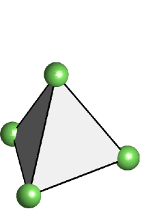
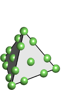
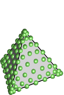
$N_{p}$ = 1	$N_{p}$ = 3	$N_{p}$ = 8

Figure 1: Warp & blend tetrahedral nodal point distribution for $N_{p}$ = 1, 3, 8. For clarity only facial nodes are illustrated.

The medium coefficients are expanded in a likewise manner

$$\begin{split}(\textbf{\em C}_{h})_{ij}(\textbf{\em x})=&\bigoplus_{{D^{\mathrm{e}}}}\sum_{n=1}^{N_{p}}(\textbf{\em C}_{h,n}^{{D^{\mathrm{e}}_{\scriptscriptstyle\mathrm{S}}}})_{ij}\phi_{n}(\textbf{\em x}),\\ \mbox{with }(\textbf{\em C}_{h,n}^{{D^{\mathrm{e}}_{\scriptscriptstyle\mathrm{S}}}})_{ij}=&(\textbf{\em C}_{h})_{ij}(\textbf{\em x}_{n}),n=1,2,\cdots,N_{\mathrm{dof}}^{D^{e}},\end{split}$$ (23)

and similarly for $\rho,\widetilde{\rho},\widetilde{\lambda}$. When refining a mesh, we expect an increase in number of elements ${D^{\mathrm{e}}}$ with decreased size.

3.3 The system of equations in matrix form

To simplify the notation in the further development of a numerical scheme, we introduce a joint matrix form of the system of equations. We map the components of $\textbf{\em E},\textbf{\em v}$ and $\widetilde{E},\widetilde{\textbf{\em v}}$ to $9\times 1$ and $4\times 1$ matrices, respectively,

$$\textbf{\em q}=(E_{11},E_{22},E_{33},E_{23},E_{13},E_{12},v_{1},v_{2},v_{3})^{T}\quad\text{and}\quad\widetilde{\textbf{\em q}}=(\widetilde{E},\widetilde{v}_{1},\widetilde{v}_{2},\widetilde{v}_{3})^{T},$$ (24)

and, correspondingly, the components of body forces f and $\widetilde{f}$ to the matrix

$$\textbf{\em g}=(0,0,0,0,0,0,f_{1},f_{2},f_{3})^{T}\quad\text{and}\quad\widetilde{\textbf{\em g}}=\left(-\frac{\widetilde{f}}{\widetilde{\lambda}},0,0,0\right)^{T}\quad.$$

Equations (2) and (3) attain the form

$${\mathbfcal{Q}}\,\frac{\partial\textbf{\em q}}{\partial t}-\nabla\cdot(\mathcal{A}\textbf{\em q})=\textbf{\em g}\quad\mbox{and}\quad\widetilde{{\mathbfcal{Q}}}\,\frac{\partial\widetilde{\textbf{\em q}}}{\partial t}-\nabla\cdot(\widetilde{\mathcal{A}}\widetilde{\textbf{\em q}})=\widetilde{\textbf{\em g}},$$ (25)

where

$${\mathbfcal{Q}}=\left(\begin{array}[]{ccc}I_{6\times 6}&\vline&0\\ \hline\cr 0&\vline&\rho I_{3\times 3}\end{array}\right)\quad\text{and}\quad\widetilde{{\mathbfcal{Q}}}=\left(\begin{array}[]{ccc}{1}&\vline&0\\ \hline\cr 0&\vline&\widetilde{\rho}I_{3\times 3}\end{array}\right)$$

and

$$\mathcal{A}=(A_{1},A_{2},A_{3})\quad\text{and}\quad\widetilde{\mathcal{A}}=(\widetilde{A}_{1},\widetilde{A}_{2},\widetilde{A}_{3}),$$

that is,

$$\begin{split}(\nabla\cdot(\mathcal{A}\textbf{\em q}))_{l}=\partial_{x_{k}}((\mathcal{A}_{k})_{lm}\textbf{\em q}_{m})\quad\text{and}\quad(\nabla\cdot(\widetilde{\mathcal{A}}\widetilde{\textbf{\em q}}))_{l}=\partial_{x_{k}}((\widetilde{\mathcal{A}}_{k})_{lm}\widetilde{\textbf{\em q}}_{m}),\\ k=1,2,3,\quad l,m=1,\cdots,9\mbox{ or }1,\cdots,4\end{split}$$

with

$$A_{1}=\left(\begin{array}[]{ccc}{\displaystyle\mathbf{0}}&\vline&\begin{array}[]{ccc}1&0&0\\[-5.69054pt] 0&0&0\\[-5.69054pt] 0&0&0\\[-5.69054pt] 0&0&0\\[-5.69054pt] 0&0&\frac{1}{2}\\[-5.69054pt] 0&\frac{1}{2}&0\end{array}\\ \hline\cr\begin{array}[]{cccccc}C_{11}&C_{12}&C_{13}&2C_{14}&2C_{15}&2C_{16}\\[-5.69054pt] C_{16}&C_{26}&C_{36}&2C_{46}&2C_{56}&2C_{66}\\[-5.69054pt] C_{15}&C_{25}&C_{35}&2C_{45}&2C_{55}&2C_{56}\end{array}&\vline&{\displaystyle\mathbf{0}}\end{array}\right)\quad\text{and}\quad\widetilde{A}_{1}=\left(\begin{array}[]{ccc}{\displaystyle\mathbf{0}}&\vline&\begin{array}[]{ccc}1&0&0\\ 0&0&0\\ 0&0&0\end{array}\\ \hline\cr{\widetilde{\lambda}}&\vline&{\displaystyle\mathbf{0}}\end{array}\right),$$

$$A_{2}=\left(\begin{array}[]{ccc}{\displaystyle\mathbf{0}}&\vline&\begin{array}[]{ccc}0&0&0\\[-5.69054pt] 0&1&0\\[-5.69054pt] 0&0&0\\[-5.69054pt] 0&0&\frac{1}{2}\\[-5.69054pt] 0&0&0\\[-5.69054pt] \frac{1}{2}&0&0\end{array}\\ \hline\cr\begin{array}[]{cccccc}C_{16}&C_{26}&C_{36}&2C_{46}&2C_{56}&2C_{66}\\[-5.69054pt] C_{12}&C_{22}&C_{23}&2C_{24}&2C_{25}&2C_{26}\\[-5.69054pt] C_{14}&C_{24}&C_{34}&2C_{44}&2C_{45}&2C_{46}\end{array}&\vline&{\displaystyle\mathbf{0}}\end{array}\right)\quad\text{and}\quad\widetilde{A}_{2}=\left(\begin{array}[]{ccc}{\displaystyle\mathbf{0}}&\vline&\begin{array}[]{ccc}0&0&0\\ 0&1&0\\ 0&0&0\end{array}\\ \hline\cr{\widetilde{\lambda}}&\vline&{\displaystyle\mathbf{0}}\end{array}\right),$$

$$A_{3}=\left(\begin{array}[]{ccc}{\displaystyle\mathbf{0}}&\vline&\begin{array}[]{ccc}0&0&0\\[-5.69054pt] 0&0&0\\[-5.69054pt] 0&0&1\\[-5.69054pt] 0&\frac{1}{2}&0\\[-5.69054pt] \frac{1}{2}&0&0\\[-5.69054pt] 0&0&0\end{array}\\ \hline\cr\begin{array}[]{cccccc}C_{15}&C_{25}&C_{35}&2C_{45}&2C_{55}&2C_{56}\\[-5.69054pt] C_{14}&C_{24}&C_{34}&2C_{44}&2C_{45}&2C_{46}\\[-5.69054pt] C_{13}&C_{23}&C_{33}&2C_{34}&2C_{35}&2C_{36}\end{array}&\vline&{\displaystyle\mathbf{0}}\end{array}\right)\quad\text{and}\quad\widetilde{A}_{3}=\left(\begin{array}[]{ccc}{\displaystyle\mathbf{0}}&\vline&\begin{array}[]{ccc}0&0&0\\ 0&0&0\\ 0&0&1\end{array}\\ \hline\cr{\widetilde{\lambda}}&\vline&{\displaystyle\mathbf{0}}\end{array}\right).$$

We define the coefficient matrices $\mathcal{A}_{n}$ in the normal directions $\textbf{\em n}=(\,n_{1},n_{2},n_{3})$ as $\mathcal{A}_{n}=n_{1}A_{1}+n_{2}A_{2}+n_{3}A_{3}$, thus $\mathcal{A}_{n}\textbf{\em q}\equiv\textbf{\em n}\cdot(\mathcal{A}\textbf{\em q})$; similarly, $\widetilde{\mathcal{A}}_{n}=n_{1}\tilde{A}_{1}+n_{2}\tilde{A}_{2}+n_{3}\tilde{A}_{3}$. We can also give them in the matrix form,

$$\mathcal{A}_{n}=\left(\begin{array}[]{cc}0&T_{12}\\ T_{21}\cdot\textbf{\em C}&0\end{array}\right)\quad\text{and}\quad\widetilde{\mathcal{A}}_{n}=\left(\begin{array}[]{cc}0&\textbf{\em n}^{T}\\ {\widetilde{\lambda}}\textbf{\em n}&0\end{array}\right),$$

with

$$T_{12}=\left(\begin{array}[]{cccccc}n_{1}&0&0&0&\tfrac{1}{2}n_{3}&\tfrac{1}{2}n_{2}\\ 0&n_{2}&0&\tfrac{1}{2}n_{3}&0&\tfrac{1}{2}n_{1}\\ 0&0&n_{3}&\tfrac{1}{2}n_{2}&\tfrac{1}{2}n_{1}&0\end{array}\right)^{T},\quad T_{21}=\left(\begin{array}[]{cccccc}n_{1}&0&0&0&n_{3}&n_{2}\\ 0&n_{2}&0&n_{3}&0&n_{1}\\ 0&0&n_{3}&n_{2}&n_{1}&0\end{array}\right).$$

We introduce

$${\Lambda}=\left(\begin{array}[]{ccc}\textbf{\em C}&\vline&0\\ \hline\cr 0&\vline&I_{3\times 3}\end{array}\right)\quad\text{and}\quad\widetilde{{\Lambda}}=\left(\begin{array}[]{ccc}\widetilde{\lambda}&\vline&0\\ \hline\cr 0&\vline&I_{3\times 3}\end{array}\right).$$

In the solid regions, we write $\textbf{\em p}={\left(H_{11},H_{22},H_{33},H_{23},H_{13},H_{12},w_{1},w_{2},w_{3}\right)}^{T}$, and in the fluid regions, we write $\widetilde{\textbf{\em p}}=(\widetilde{H},\tilde{w}_{1},\tilde{w}_{2},\tilde{w}_{3})^{T}$. The inner product $(\textbf{\em q},\textbf{\em p})_{\Omega}$ indicates the dot product of vectors q and p followed by integration over the domain $\Omega$. Equation (9) is then rewritten, regarding the supports of basis functions $\textbf{\em p}_{h}$ localized to an element ${D^{\mathrm{e}}}_{\mathrm{S},\mathrm{F}}$, as

$$\begin{split}({\mathbfcal{Q}}_{h}\frac{\partial\textbf{\em q}_{h}}{\partial t},{{\Lambda}_{h}}\textbf{\em p}_{h})_{{D^{\mathrm{e}}_{\scriptscriptstyle\mathrm{S}}}}-&(\nabla\cdot(\mathcal{A}_{h}\textbf{\em q}_{h}),{{\Lambda}_{h}}\textbf{\em p}_{h})_{{D^{\mathrm{e}}_{\scriptscriptstyle\mathrm{S}}}}-\tfrac{1}{2}({\,[\![\mathcal{A}_{n,h}\textbf{\em q}_{h}\,]\!]}_{\scriptscriptstyle\mathrm{SS}},({\Lambda}_{h}\textbf{\em p}_{h})^{-})_{\Sigma_{{\scriptscriptstyle\mathrm{SS}}}^{\mathrm{e}}}\\ -&\tfrac{1}{2}({\,[\![\mathcal{A}_{n,h}\textbf{\em q}_{h}\,]\!]}_{\scriptscriptstyle\mathrm{SF}},({\Lambda}_{h}\textbf{\em p}_{h})^{-})_{\Sigma_{{\scriptscriptstyle\mathrm{SF}}}^{\mathrm{e}}}=(\textbf{\em g},{{\Lambda}_{h}}\textbf{\em p}_{h})_{{D^{\mathrm{e}}_{\scriptscriptstyle\mathrm{S}}}},\end{split}$$ (26)

$$\begin{split}(\widetilde{{\mathbfcal{Q}}}_{h}\frac{\partial\widetilde{\textbf{\em q}}_{h}}{\partial t},{\widetilde{{\Lambda}}_{h}}\widetilde{\textbf{\em p}}_{h})_{{D^{\mathrm{e}}_{\scriptscriptstyle\mathrm{F}}}}-&(\nabla\cdot(\widetilde{\mathcal{A}}_{h}\widetilde{\textbf{\em q}}_{h}),{\widetilde{{\Lambda}}_{h}}\widetilde{\textbf{\em p}}_{h})_{{D^{\mathrm{e}}_{\scriptscriptstyle\mathrm{F}}}}-\tfrac{1}{2}({\,[\![\widetilde{\mathcal{A}}_{n,h}\widetilde{\textbf{\em q}}_{h}\,]\!]}_{\scriptscriptstyle\mathrm{FF}},(\widetilde{{\Lambda}}_{h}\widetilde{\textbf{\em p}}_{h})^{-})_{\Sigma_{{\scriptscriptstyle\mathrm{FF}}}^{\mathrm{e}}}\\ -&\tfrac{1}{2}({\,[\![\widetilde{\mathcal{A}}_{n,h}\widetilde{\textbf{\em q}}_{h}\,]\!]}_{\scriptscriptstyle\mathrm{FS}},(\widetilde{{\Lambda}}_{h}\widetilde{\textbf{\em p}}_{h})^{-})_{\Sigma_{{\scriptscriptstyle\mathrm{FS}}}^{\mathrm{e}}}=(\widetilde{\textbf{\em g}},{\widetilde{{\Lambda}}_{h}}\widetilde{\textbf{\em p}}_{h})_{{D^{\mathrm{e}}_{\scriptscriptstyle\mathrm{F}}}}.\end{split}$$ (27)

In the above we identify the central flux as

$$\mathcal{F}^{\mathrm{C}}_{\mathrm{S}*}=\tfrac{1}{2}({\,[\![\mathcal{A}_{n}\textbf{\em q}\,]\!]}_{\mathrm{S}*},({\Lambda}\textbf{\em p})^{-})_{\Sigma_{\mathrm{S}*}^{\mathrm{e}}},\quad\widetilde{\mathcal{F}}^{\mathrm{C}}_{\mathrm{F}*}=\tfrac{1}{2}({\,[\![\widetilde{\mathcal{A}}_{n}\widetilde{\textbf{\em q}}\,]\!]}_{\mathrm{F}*},(\widetilde{{\Lambda}}\widetilde{\textbf{\em p}})^{-})_{\Sigma_{\mathrm{F}*}^{\mathrm{e}}},\quad*\in\{\mathrm{S,F}\},$$ (28)

in which we redefine

$$\begin{split}&{\,[\![\mathcal{A}_{n}\textbf{\em q}\,]\!]}_{\scriptscriptstyle\mathrm{SS}}=(\mathcal{A}_{n}\textbf{\em q})^{+}-(\mathcal{A}_{n}\textbf{\em q})^{-},\quad{\,[\![\mathcal{A}_{n}\textbf{\em q}\,]\!]}_{\scriptscriptstyle\mathrm{SF}}=O^{T}(\widetilde{\mathcal{A}}_{n}\widetilde{\textbf{\em q}})^{+}-(\mathcal{A}_{n}\textbf{\em q})^{-},\\ &{\,[\![\widetilde{\mathcal{A}}_{n}\widetilde{\textbf{\em q}}\,]\!]}_{\scriptscriptstyle\mathrm{FF}}=(\widetilde{\mathcal{A}}_{n}\widetilde{\textbf{\em q}})^{+}-(\widetilde{\mathcal{A}}_{n}\widetilde{\textbf{\em q}})^{-},\quad{\,[\![\widetilde{\mathcal{A}}_{n}\widetilde{\textbf{\em q}}\,]\!]}_{\scriptscriptstyle\mathrm{FS}}=O^{\phantom{*}}(\mathcal{A}_{n}\textbf{\em q})^{+}-(\widetilde{\mathcal{A}}_{n}\widetilde{\textbf{\em q}})^{-},\end{split}$$ (29)

with the map $O:\mathbb{R}^{9}\to\mathbb{R}^{4}$ given by

$$O\textbf{\em q}=\left(\begin{array}[]{c}\textbf{\em n}\cdot\textbf{\em E}\cdot\textbf{\em n}\\ (\textbf{\em n}\cdot\textbf{\em v})\textbf{\em n}\end{array}\right),\quad\mbox{ and its adjoint }\quad O^{T}\widetilde{\textbf{\em q}}=\left(\begin{array}[]{c}(\textbf{\em n}\textbf{\em n})\widetilde{E}\\ (\textbf{\em n}\cdot\widetilde{\textbf{\em v}})\textbf{\em n}\end{array}\right),$$

which can also be explicitly given in the matrix form

$$O=\left(\begin{array}[]{ccc}\begin{array}[]{cccccc}n_{1}n_{1}&n_{2}n_{2}&n_{3}n_{3}&n_{2}n_{3}&n_{1}n_{3}&n_{1}n_{2}\end{array}&\vline&{\displaystyle\mathbf{0}}\\ \hline\cr{\displaystyle\mathbf{0}}&\vline&\begin{array}[]{ccc}n_{1}n_{1}&n_{1}n_{2}&n_{1}n_{3}\\[-5.69054pt] n_{1}n_{2}&n_{2}n_{2}&n_{2}n_{3}\\[-5.69054pt] n_{1}n_{3}&n_{2}n_{3}&n_{3}n_{3}\end{array}\end{array}\right).$$

4 The Boundary Condition penalized numerical flux and stability

Here, we construct our penalized numerical flux. The flux is designed such that the penalized discrete counterpart of the weak form (26) and (27) satisfies the condition of non-increasing energy and guarantees a proper error estimate. We replace the central fluxes, $\mathcal{F}^{\mathrm{C}}$ and $\widetilde{\mathcal{F}}^{\mathrm{C}}$, in (28), by penalized fluxes, $\mathcal{F}^{\mathrm{P}}$ and $\widetilde{\mathcal{F}}^{\mathrm{P}}$, by adding penalty terms, that is:

$$\begin{split}\mathcal{F}^{\mathrm{P}}_{\mathrm{S}*}=&\tfrac{1}{2}({\,[\![\mathcal{A}_{n}\textbf{\em q}\,]\!]}_{\mathrm{S}*},({\Lambda}\textbf{\em p})^{-})_{\Sigma_{\mathrm{S}*}^{\mathrm{e}}}+\alpha(\mathcal{A}_{n}^{T,{-}}{\,[\![\mathcal{A}_{n}\textbf{\em q}\,]\!]}_{\mathrm{S}*},\textbf{\em p}^{-})_{\Sigma_{\mathrm{S}*}^{\mathrm{e}}}\\ &=\tfrac{1}{2}({\,[\![\mathcal{A}_{n}\textbf{\em q}\,]\!]}_{\mathrm{S}*},({\Lambda}\textbf{\em p})^{-})_{\Sigma_{\mathrm{S}*}^{\mathrm{e}}}+\alpha({\,[\![\mathcal{A}_{n}\textbf{\em q}\,]\!]}_{\mathrm{S}*},(\mathcal{A}_{n}\textbf{\em p})^{-})_{\Sigma_{\mathrm{S}*}^{\mathrm{e}}},\\ \widetilde{\mathcal{F}}^{\mathrm{P}}_{\mathrm{F}*}=&\tfrac{1}{2}({\,[\![\widetilde{\mathcal{A}}_{n}\widetilde{\textbf{\em q}}\,]\!]}_{\mathrm{F}*},(\widetilde{{\Lambda}}\widetilde{\textbf{\em p}})^{-})_{\Sigma_{\mathrm{F}*}^{\mathrm{e}}}+\alpha(\widetilde{\mathcal{A}}_{n}^{T,{-}}{\,[\![\widetilde{\mathcal{A}}_{n}\widetilde{\textbf{\em q}}\,]\!]}_{\mathrm{F}*},\widetilde{\textbf{\em p}}^{-})_{\Sigma_{\mathrm{F}*}^{\mathrm{e}}}\\ &=\tfrac{1}{2}({\,[\![\widetilde{\mathcal{A}}_{n}\widetilde{\textbf{\em q}}\,]\!]}_{\mathrm{F}*},(\widetilde{{\Lambda}}\widetilde{\textbf{\em p}})^{-})_{\Sigma_{\mathrm{F}*}^{\mathrm{e}}}+\alpha({\,[\![\widetilde{\mathcal{A}}_{n}\widetilde{\textbf{\em q}}\,]\!]}_{\mathrm{F}*},(\widetilde{\mathcal{A}}_{n}\widetilde{\textbf{\em p}})^{-})_{\Sigma_{\mathrm{F}*}^{\mathrm{e}}},\quad*\in\{\mathrm{S},\mathrm{F}\}\end{split}$$ (30)

with $\alpha$ some positive constant scalar. With this modification, (26) and (27) becomes

$$\begin{aligned} ({\mathbfcal{Q}}_{h}\frac{\partial\textbf{\em q}_{h}}{\partial t},{{\Lambda}_{h}}\textbf{\em p}_{h})_{{D^{\mathrm{e}}_{\scriptscriptstyle\mathrm{S}}}}-&(\nabla\cdot(\mathcal{A}_{h}\textbf{\em q}_{h}),{{\Lambda}_{h}}\textbf{\em p}_{h})_{{D^{\mathrm{e}}_{\scriptscriptstyle\mathrm{S}}}}-\tfrac{1}{2}({\,[\![\mathcal{A}_{n,h}\textbf{\em q}_{h}\,]\!]}_{\mathrm{S}*},({\Lambda}_{h}\textbf{\em p}_{h})^{-})_{\Sigma_{\mathrm{S}*}^{\mathrm{e}}}\\ -&\alpha({\,[\![\mathcal{A}_{n,h}\textbf{\em q}_{h}\,]\!]}_{\mathrm{S}*},(\mathcal{A}_{n,h}\textbf{\em p}_{h})^{-})_{\Sigma_{\mathrm{S}*}^{\mathrm{e}}}=(\textbf{\em g},{{\Lambda}_{h}}\textbf{\em p}_{h})_{{D^{\mathrm{e}}_{\scriptscriptstyle\mathrm{S}}}},\end{aligned}$$ (31)

$$\begin{aligned} (\widetilde{{\mathbfcal{Q}}}_{h}\frac{\partial\widetilde{\textbf{\em q}}_{h}}{\partial t},{\widetilde{{\Lambda}}_{h}}\widetilde{\textbf{\em p}}_{h})_{{D^{\mathrm{e}}_{\scriptscriptstyle\mathrm{F}}}}-&(\nabla\cdot(\widetilde{\mathcal{A}}_{h}\widetilde{\textbf{\em q}}_{h}),{\widetilde{{\Lambda}}_{h}}\widetilde{\textbf{\em p}}_{h})_{{D^{\mathrm{e}}_{\scriptscriptstyle\mathrm{F}}}}-\tfrac{1}{2}({\,[\![\widetilde{\mathcal{A}}_{n,h}\widetilde{\textbf{\em q}}_{h}\,]\!]}_{\mathrm{F}*},(\widetilde{{\Lambda}}_{h}\widetilde{\textbf{\em p}}_{h})^{-})_{\Sigma_{\mathrm{F}*}^{\mathrm{e}}}\\ -&\alpha({\,[\![\widetilde{\mathcal{A}}_{n,h}\widetilde{\textbf{\em q}}_{h}\,]\!]}_{\mathrm{F}*},(\widetilde{\mathcal{A}}_{n,h}\widetilde{\textbf{\em p}}_{h})^{-})_{\Sigma_{\mathrm{F}*}^{\mathrm{e}}}=(\widetilde{\textbf{\em g}},{\widetilde{{\Lambda}}_{h}}\widetilde{\textbf{\em p}}_{h})_{{D^{\mathrm{e}}_{\scriptscriptstyle\mathrm{F}}}},\quad*\in\{\mathrm{S},\mathrm{F}\}.\end{aligned}$$ (32)

In Appendix A we provide a guideline how to choose an $\alpha$ based on an error analysis. We set $\alpha=1/2$, in which case the energy function with the penalty terms coincides with the one using an upwind flux [Warburton(2013)]. For the convergence analysis, we follow [Warburton(2013), Section 5.1] while obtaining an error estimate.

Following the matrix form in Subsection 3.3, we immediately rewrite the definition of energy functions (13) in solid and fluid region as

$$\begin{split}{\mathcal{E}}_{\mathrm{S},h}=&\tfrac{1}{2}{\sum_{\mathrm{e}}}({\mathbfcal{Q}}_{h}\textbf{\em q}_{h},{\Lambda}_{h}\textbf{\em q}_{h})_{D^{\mathrm{e}}_{\scriptscriptstyle\mathrm{S}}}=\tfrac{1}{2}{\sum_{\mathrm{e}}}{\left\|\textbf{\em q}\,\right\|}_{L^{2}({D^{\mathrm{e}}_{\scriptscriptstyle\mathrm{S}}};{\mathbfcal{Q}}_{h},{\Lambda}_{h})}\\ {\mathcal{E}}_{\mathrm{F},h}=&\tfrac{1}{2}{\sum_{\mathrm{e}}}(\widetilde{{\mathbfcal{Q}}}_{h}\widetilde{\textbf{\em q}}_{h},\widetilde{{\Lambda}}_{h}\widetilde{\textbf{\em q}}_{h})_{D^{\mathrm{e}}_{\scriptscriptstyle\mathrm{F}}}=\tfrac{1}{2}{\sum_{\mathrm{e}}}{\left\|\widetilde{\textbf{\em q}}\,\right\|}_{L^{2}({D^{\mathrm{e}}_{\scriptscriptstyle\mathrm{F}}};\widetilde{{\mathbfcal{Q}}}_{h},\widetilde{{\Lambda}}_{h})}.\end{split}$$ (33)

Here ${\|\centerdot\,\|}_{L^{2}({D^{\mathrm{e}}_{\scriptscriptstyle\mathrm{S}}};{\mathbfcal{Q}},{\Lambda})}$ and ${\|\centerdot\,\|}_{L^{2}({D^{\mathrm{e}}_{\scriptscriptstyle\mathrm{F}}};\widetilde{{\mathbfcal{Q}}},\widetilde{{\Lambda}})}$ are the energy norms in solid and fluid regions, and we simplify the notification without causing ambiguity by ${\|\centerdot\,\|}\phantom{|}_{L^{2}({D^{\mathrm{e}}_{\scriptscriptstyle\mathrm{S}}};\,{\mathbfcal{Q}},{\Lambda})}$ and ${\|\centerdot\,\|}\phantom{|}_{L^{2}({D^{\mathrm{e}}_{\scriptscriptstyle\mathrm{F}}};\,\widetilde{{\mathbfcal{Q}}},\widetilde{{\Lambda}})}$, respectively. We also define the energy norms in solid-solid, fluid-fluid and solid-fluid interfaces similarly as ${\|\centerdot\,\|}_{L^{2}({\Sigma_{{\scriptscriptstyle\mathrm{SS}}}^{\mathrm{e}}})}$, ${\|\centerdot\,\|}_{L^{2}({\Sigma_{{\scriptscriptstyle\mathrm{FF}}}^{\mathrm{e}}})}$ and ${\|\centerdot\,\|}_{L^{2}({\Sigma_{{\scriptscriptstyle\mathrm{SF}}}^{\mathrm{e}}})}$, ${\|\centerdot\,\|}_{L^{2}({\Sigma_{{\scriptscriptstyle\mathrm{FS}}}^{\mathrm{e}}})}$. Upon taking the penalty terms into consideration, equation (16) is replaced by

$$\begin{split}&\frac{\,\mathrm{d}{\mathcal{E}}_{h}}{\,\mathrm{d}t}+\frac{\alpha}{2}\Bigl{(}{\sum_{\mathrm{e}}}{\|{\,[\![\mathcal{A}_{n,h}\textbf{\em q}_{h}\,]\!]}_{\scriptscriptstyle\mathrm{SS}}\,\|}_{L^{2}({\Sigma_{{\scriptscriptstyle\mathrm{SS}}}^{\mathrm{e}}})}^{2}+{\sum_{\mathrm{e}}}{\|{\,[\![\widetilde{\mathcal{A}}_{n,h}\widetilde{\textbf{\em q}}_{h}\,]\!]}_{\scriptscriptstyle\mathrm{FF}}\,\|}_{L^{2}({\Sigma_{{\scriptscriptstyle\mathrm{FF}}}^{\mathrm{e}}})}^{2}\\ &\hskip 28.45274pt+2{\sum_{\mathrm{e}}}{\|{\,[\![\mathcal{A}_{n,h}\textbf{\em q}_{h}\,]\!]}_{\scriptscriptstyle\mathrm{SF}}\,\|}_{L^{2}({\Sigma_{{\scriptscriptstyle\mathrm{SF}}}^{\mathrm{e}}})}^{2}\Bigr{)}={\sum_{\mathrm{e}}}\int_{D^{\mathrm{e}}_{\scriptscriptstyle\mathrm{S}}}\textbf{\em g}_{h}\cdot{\Lambda}_{h}\textbf{\em q}_{h}\,\mathrm{d}\Omega+{\sum_{\mathrm{e}}}\int_{D^{\mathrm{e}}_{\scriptscriptstyle\mathrm{F}}}\widetilde{\textbf{\em g}}_{h}\cdot\widetilde{{\Lambda}}_{h}\widetilde{\textbf{\em q}}_{h}\,\mathrm{d}\Omega.\end{split}$$ (34)

To obtain this result, in (31) – (32), we let $\textbf{\em p}=\textbf{\em q},\widetilde{\textbf{\em p}}=\widetilde{\textbf{\em q}}$. Taking the summation over all penalty terms on solid-solid interfaces yields

$$\begin{split}{\sum_{\mathrm{e}}}({\,[\![\mathcal{A}_{n,h}\textbf{\em q}_{h}\,]\!]}_{\scriptscriptstyle\mathrm{SS}},(\mathcal{A}_{n,h}\textbf{\em q}_{h})^{-})_{\Sigma_{{\scriptscriptstyle\mathrm{SS}}}^{\mathrm{e}}}&=\hskip 17.07164pt{\sum_{\mathrm{e}}}((\mathcal{A}_{n,h}\textbf{\em q}_{h})^{+}-(\mathcal{A}_{n,h}\textbf{\em q}_{h})^{-},(\mathcal{A}_{n,h}\textbf{\em q}_{h})^{-})_{\Sigma_{{\scriptscriptstyle\mathrm{SS}}}^{\mathrm{e}}}\\ &=-\tfrac{1}{2}{\sum_{\mathrm{e}}}{\|{\,[\![\mathcal{A}_{n,h}\textbf{\em q}_{h}\,]\!]}_{\scriptscriptstyle\mathrm{SS}}\,\|}_{L^{2}({\Sigma_{{\scriptscriptstyle\mathrm{SS}}}^{\mathrm{e}}})}^{2}\end{split}$$ (35)

Taking the summation over all penalty terms on fluid-fluid interfaces yields

$${\sum_{\mathrm{e}}}({\,[\![\widetilde{\mathcal{A}}_{n,h}\widetilde{\textbf{\em q}}_{h}\,]\!]}_{\scriptscriptstyle\mathrm{FF}},(\widetilde{\mathcal{A}}_{n,h}\widetilde{\textbf{\em q}}_{h})^{-})_{\Sigma_{{\scriptscriptstyle\mathrm{FF}}}^{\mathrm{e}}}=-\tfrac{1}{2}{\sum_{\mathrm{e}}}{\|{\,[\![\widetilde{\mathcal{A}}_{n,h}\widetilde{\textbf{\em q}}_{h}\,]\!]}_{\scriptscriptstyle\mathrm{FF}}\,\|}_{L^{2}({\Sigma_{{\scriptscriptstyle\mathrm{FF}}}^{\mathrm{e}}})}^{2}.$$ (36)

We rewrite the penalty terms on fluid-solid interface from the solid side as

$$\begin{split}&({\,[\![\mathcal{A}_{n,h}\textbf{\em q}_{h}\,]\!]}_{\scriptscriptstyle\mathrm{SF}},(\mathcal{A}_{n,h}\textbf{\em q}_{h})^{-})_{\Sigma_{{\scriptscriptstyle\mathrm{SF}}}^{\mathrm{e}}}\\ =&(O^{T}(\widetilde{\mathcal{A}}_{n,h}\widetilde{\textbf{\em q}}_{h})^{+},(\mathcal{A}_{n,h}\textbf{\em q}_{h})^{-})_{\Sigma_{{\scriptscriptstyle\mathrm{SF}}}^{\mathrm{e}}}-((\mathcal{A}_{n,h}\textbf{\em q}_{h})^{-},(\mathcal{A}_{n,h}\textbf{\em q}_{h})^{-})_{\Sigma_{{\scriptscriptstyle\mathrm{SF}}}^{\mathrm{e}}},\end{split}$$ (37)

and from the fluid side as

$$\begin{split}&({\,[\![\widetilde{\mathcal{A}}_{n,h}\widetilde{\textbf{\em q}}_{h}\,]\!]}_{\scriptscriptstyle\mathrm{FS}},(\widetilde{\mathcal{A}}_{n,h}\widetilde{\textbf{\em q}}_{h})^{-})_{\Sigma_{{\scriptscriptstyle\mathrm{FS}}}^{\mathrm{e}}}\\ =&(O(\mathcal{A}_{n,h}\textbf{\em q}_{h})^{+},(\widetilde{\mathcal{A}}_{n,h}\widetilde{\textbf{\em q}}_{h})^{-})_{\Sigma_{{\scriptscriptstyle\mathrm{FS}}}^{\mathrm{e}}}-((\widetilde{\mathcal{A}}_{n,h}\widetilde{\textbf{\em q}}_{h})^{-},(\widetilde{\mathcal{A}}_{n,h}\widetilde{\textbf{\em q}}_{h})^{-})_{\Sigma_{{\scriptscriptstyle\mathrm{FS}}}^{\mathrm{e}}}\\ =&((\mathcal{A}_{n,h}\textbf{\em q}_{h})^{+},O^{T}(\widetilde{\mathcal{A}}_{n,h}\widetilde{\textbf{\em q}}_{h})^{-})_{\Sigma_{{\scriptscriptstyle\mathrm{FS}}}^{\mathrm{e}}}-(O^{T}(\widetilde{\mathcal{A}}_{n,h}\widetilde{\textbf{\em q}}_{h})^{-},O^{T}(\widetilde{\mathcal{A}}_{n,h}\widetilde{\textbf{\em q}}_{h})^{-})_{\Sigma_{{\scriptscriptstyle\mathrm{FS}}}^{\mathrm{e}}},\end{split}$$ (38)

in which the property $OO^{T}=I_{4\times 4}$ is used. Changing from the fluid to the solid sides yields

$$\begin{split}&({\,[\![\widetilde{\mathcal{A}}_{n,h}\widetilde{\textbf{\em q}}_{h}\,]\!]}_{\scriptscriptstyle\mathrm{FS}},(\widetilde{\mathcal{A}}_{n,h}\widetilde{\textbf{\em q}}_{h})^{-})_{\Sigma_{{\scriptscriptstyle\mathrm{FS}}}^{\mathrm{e}}}\\ =&((\mathcal{A}_{n,h}\textbf{\em q}_{h})^{-},O^{T}(\widetilde{\mathcal{A}}_{n,h}\widetilde{\textbf{\em q}}_{h})^{+})_{\Sigma_{{\scriptscriptstyle\mathrm{SF}}}^{\mathrm{e}}}-(O^{T}(\widetilde{\mathcal{A}}_{n,h}\widetilde{\textbf{\em q}}_{h})^{+},O^{T}(\widetilde{\mathcal{A}}_{n,h}\widetilde{\textbf{\em q}}_{h})^{+})_{\Sigma_{{\scriptscriptstyle\mathrm{SF}}}^{\mathrm{e}}}.\end{split}$$ (39)

Summation over all fluid-solid interfaces with (37) and (39),

$$\begin{split}&{\sum_{\mathrm{e}}}({\,[\![\mathcal{A}_{n,h}\textbf{\em q}_{h}\,]\!]}_{\scriptscriptstyle\mathrm{SF}},(\mathcal{A}_{n,h}\textbf{\em q}_{h})^{-})_{\Sigma_{{\scriptscriptstyle\mathrm{SF}}}^{\mathrm{e}}}+{\sum_{\mathrm{e}}}({\,[\![\widetilde{\mathcal{A}}_{n,h}\widetilde{\textbf{\em q}}_{h}\,]\!]}_{\scriptscriptstyle\mathrm{FS}},(\widetilde{\mathcal{A}}_{n,h}\widetilde{\textbf{\em q}}_{h})^{-})_{\Sigma_{{\scriptscriptstyle\mathrm{FS}}}^{\mathrm{e}}}\\ &\hskip 28.45274pt=-{\sum_{\mathrm{e}}}{\|O^{T}(\widetilde{\mathcal{A}}_{n,h}\widetilde{\textbf{\em q}}_{h})^{+}-(\mathcal{A}_{n,h}\textbf{\em q}_{h})^{-}\,\|}_{L^{2}({\Sigma_{{\scriptscriptstyle\mathrm{SF}}}^{\mathrm{e}}})}^{2}\\ &\hskip 28.45274pt=-{\sum_{\mathrm{e}}}{\|{\,[\![\mathcal{A}_{n,h}\textbf{\em q}_{h}\,]\!]}_{\scriptscriptstyle\mathrm{SF}}\,\|}_{L^{2}({\Sigma_{{\scriptscriptstyle\mathrm{SF}}}^{\mathrm{e}}})}^{2}.\end{split}$$ (40)

Thus we obtain (34).

Our approach is reminiscent of earlier work, in which an upwind flux is defined by the Riemann solutions which are obtained by diagonalizing $\mathcal{A}_{n}$, that is, $\mathcal{A}_{n}=RDR^{T}$, on the faces of each element [[Wilcox et al.(2010)Wilcox, Stadler, Burstedde, & Ghattas]], and $D$ is the diagonal matrix of eigenvalues of $\mathcal{A}_{n}$. The upwind flux takes the form,

$$\begin{split}&\mathcal{F}^{\mathrm{U}}_{\mathrm{S}*}=({\,[\![\mathcal{A}_{n}\textbf{\em q}\,]\!]}_{\mathrm{S}*},({\Lambda}\textbf{\em p})^{-})_{\Sigma_{\mathrm{S}*}^{\mathrm{e}}}+({\,[\![(R|D|R^{T})\textbf{\em q}\,]\!]}_{\mathrm{S}*},({\Lambda}\textbf{\em p})^{-})_{\Sigma_{\mathrm{S}*}^{\mathrm{e}}},\\ &\widetilde{\mathcal{F}}^{\mathrm{U}}_{\mathrm{F}*}=({\,[\![\widetilde{\mathcal{A}}_{n}\widetilde{\textbf{\em q}}\,]\!]}_{\mathrm{F}*},(\widetilde{{\Lambda}}\widetilde{\textbf{\em p}})^{-})_{\Sigma_{\mathrm{F}*}^{\mathrm{e}}}+({\,[\![(\widetilde{R}|\widetilde{D}|\widetilde{R}^{T})\widetilde{\textbf{\em q}}\,]\!]}_{\mathrm{F}*},(\widetilde{{\Lambda}}\widetilde{\textbf{\em p}})^{-})_{\Sigma_{\mathrm{F}*}^{\mathrm{e}}},\quad*\in\{\mathrm{S},\mathrm{F}\},\end{split}$$ (41)

where $|\centerdot|$ stands for the operaton of taking the absolute value of each entry of the diagonal matrix, that is, $|D|_{ij}=|D_{ij}|$. Our approach avoids this diagonalization, allowing general heterogeneous media with anisotropy.

5 Time Discretization

In this section, we discuss a time discretization that is computationally efficient for complex domains. Often, the computational meshes used to model the subsurface must contain regions where the characteristic lengths of the elements drop far below that of a wavelength because the subsurface contains very complex geometries and discontinuities. As a result, the time steps must be equally reduced to produce a stable solution. We follow two different time discretization schemes: (1) for non-complex domains, it is advantageous to use a traditional Runge–Kutta (RK) method and (2) for complex domains, a semi implicit–explicit (IMEX) method is used. The IMEX method enables the solver to perform implicit time integration in areas of oversampling, while keeping the computational efficiency of RK in regions of proper sampling.

5.1 Explicit Runge–Kutta

We use an explicit time integration method when the variation in element size is small. There are a variety of time-stepping methods available, however, we employ the five stage low-storage explicit Runge–Kutta (LSERK) method from [Cockburn & Shu(2001)]. LSERK is an explicit method the time-step of which is dictated by the Courant–Friedrichs–Lewy (CFL) condition. Efforts to define, quantitatively, a stable CFL condition depending on polynomial order $N_{p}$, can be found in [Cockburn & Shu(2001)]. The LSERK method is preferred over other methods because it saves memory at the cost of computation time.

5.2 Explicit–Implicit Runge–Kutta

When the domain in question contains complex geometries within large domains, such as rough surfaces, the resulting mesh will contain regions of oversampling relative to the relevant wavelengths. This hinders the use of an implicit time-stepping method because its accuracy depends on the size of the time step, which in turn is dependent on the region of highest spatial sampling. A natural approach is the IMEX method, (e.g. [Ascher et al.(1997)Ascher, Ruuth, & Spiteri, Kanevsky et al.(2007)Kanevsky, Carpenter, Gottlieb, & Hesthaven, Persson(2011)]), which allows the regions of oversampling to be integrated in time with an L-stable third-order and 3-stage Diagonally Implicit Runge–Kutta (DIRK) method, while using a fast and simple 4-stage third-order ERK method in the regions of more reasonable sampling (8–10 nodes per wavelength).

The system can be solved without requiring an interpolation at the boundary of the implicit–explicit regions. The intermediate abscissaes of each time step for implicit Runge–Kutta stages and for explicit ones are selected to equal one another so as to synchronize the explicit and implicit schemes, and the so-called Butcher matrix is calculated correspondingly. The implicit stages are solved using a multifrontal factorization.

6 Computational experiments

Here, we illustrate our DG method by verifying its convergence rate and carrying out computational experiments. We use the fourth-order LSERK algorithm for time integration. For visualization of wavefields or model parameters, we write the value in the Visualization Toolkit (VTK) unstructured mesh format and visualize the result using Paraview [Henderson(2007)].

6.1 Convergence tests at (interior) boundaries

We carry out computational tests using wave propagation and scattering problems in 3-dimensional cubic subdomains. We first test the propagation of a plane wave in a homogeneous isotropic elastic medium, in which periodic boundary conditions are applied. We also test the free-surface boundary condition with a homogeneous isotropic elastic solid, in which both Rayleigh and Love waves are generated. We focus on the Rayleigh wave, the particle motion of which is in the plane perpendicular to the free surface. A Stoneley wave, generated at a solid-elastic interface [Achenbach(1973)] in an unbounded domain composed of two half spaces with different material properties, is also simulated and compared with the closed-form solution in [Kaufman & Levshin(2005), Section 5.2]. For the test of our DG method at an acousto-elastic interface, we generate a Scholte wave. We refer to [Wilcox et al.(2010)Wilcox, Stadler, Burstedde, & Ghattas] for the closed-form solution. The external boundary conditions, beside those mentioned above, are imposed by using the traction of the exact solution as boundary “forces”  [Wilcox et al.(2010)Wilcox, Stadler, Burstedde, & Ghattas].

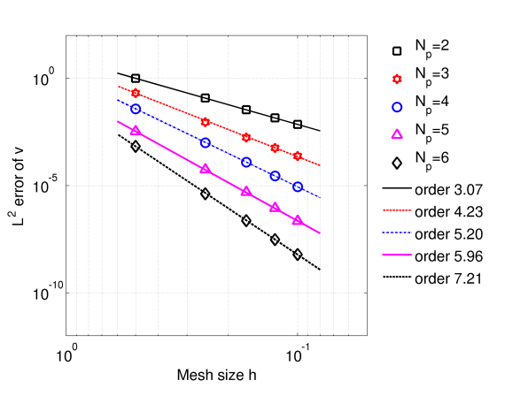
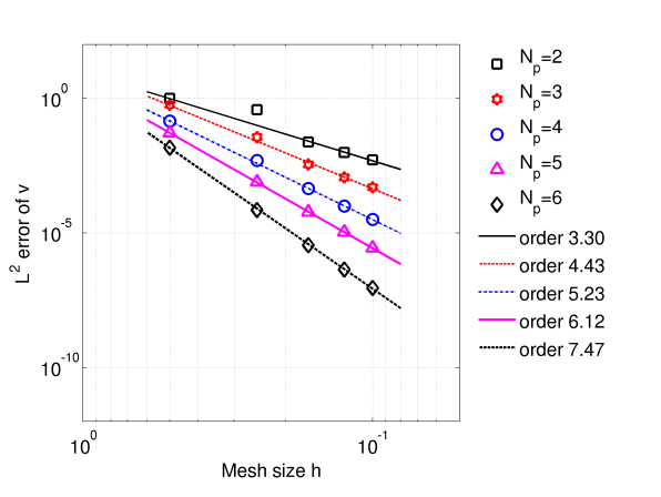
(A)	(B)
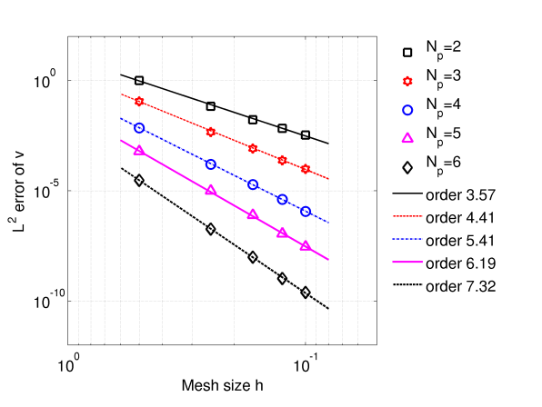
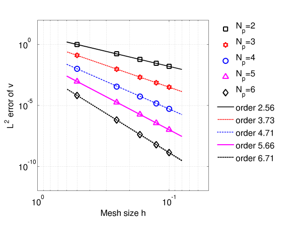
(C)	(D)

Figure 2: $L^{2}$ error of partical velocity v as a function of mesh size $h$, for the simulation of (A) a plane wave, (B) a Rayleigh wave, (C) a Stoneley wave, and (D) a Scholte wave, for different orders $N_{p}=2,3,\cdots,6$ .

The computational domains are discretized as regular tetrahedral meshes. A sufficiently small constant, $K_{\mathrm{CFL}}=0.05$, was selected during the tests for time stepping, and a large simulation time (10 s) is choosen for the error computation. The domain geometry and boundary conditions for each test are given in Table 1. The relevant material parameters, that is, the Lamé parameters $\lambda$ and $\mu$, and density $\rho$, are given in Table 2. We calculate the $L^{2}$ errors for the particle velocity of the numerical solutions, which are discretized by $N_{p}$ order polynomials. The magnitudes of the numerical errors at time $t=$ 10 s are shown in Figure 2, as a function of mesh size $h$ for different values of $N_{p}$, and least-squares fits to lines, with the estimated convergence order for each line shown in the legend. We observe that the $L^{2}$ error of our numerical scheme achieves a convergence rate higher than $N_{p}+\frac{1}{2}$. We also show a comparison of accuracies and convergence rates tested with the wave types described in this section for the upwind flux, the central flux and our penalty flux in Appendix B.

wave type	domain range (in km)	boundary conditions
plane wave	$[-1,1]\times[-1,1]\times[-1,1]$	periodic boundaries
Rayleigh wave	$[-1,1]\times[-1,1]\times[0,2]$	free surface boundary at $x_{3}=0$, exact boundary “force” at $x_{3}=2$, periodic boundaries otherwise
Stoneley wave	$[-2,2]\times[-2,2]\times[-2,2]$	exact boundary “force” at $x_{3}=\pm 2$, periodic boundaries otherwise
Scholte wave	$[-2,2]\times[-2,2]\times[-2,2]$	exact boundary “force” at $x_{3}=\pm 2$, periodic boundaries otherwise

Table 1: Geometry and boundary conditions for the four wave types in the convergence tests.

wave type	material properties
plane wave	$\lambda=2.00$ GPa, $\mu=1.00$ GPa, $\rho=1.00$ g/cm${}^{\textrm{3}}$
Rayleigh wave	$\lambda=2.00$ GPa, $\mu=1.00$ GPa, $\rho=1.00$ g/cm${}^{\textrm{3}}$
Stoneley wave	$\lambda=1.20$ Gpa, $\mu=1.20$ GPa, $\rho=1.20$ g/cm${}^{\textrm{3}}$, for $x_{3}>0$ $\lambda=3.00$ Gpa, $\mu=1.20$ GPa, $\rho=4.00$ g/cm${}^{\textrm{3}}$, for $x_{3}<0$
Scholte wave	$\lambda=1.20$ Gpa, $\mu=1.30$ GPa, $\rho=1.10$ g/cm${}^{\textrm{3}}$, for $x_{3}>0$ $\lambda=1.11$ Gpa, $\mu=0.00$ GPa, $\rho=1.32$ g/cm${}^{\textrm{3}}$, for $x_{3}<0$

Table 2: Material parameters for the four wave types in the convergence tests.

6.2 Homogeneous orthorhombic solid: Caustics

Here, we simulate a band-limited fundamental solution in an anisotropic elastic medium, forming caustics. The medium is orthorhombic and homogeneous. Several minerals in Earth’s mantle have orthorhombic symmetry; this symmetry also appears in regions of sedimentary basins where fracture sets are commonly found in sandstone beds, shales, and granites. The material properties are selected as follows,
$\rho$ $C_{11}$ $C_{22}$ $C_{33}$ $C_{44}$ $C_{55}$ $C_{66}$ $C_{23}$ $C_{13}$ $C_{12}$ 1.0 (g/cm${}^{\textrm{3}}$) 30.40 19.20 16.00 4.67 10.86 12.82 4.80 4.00 6.24 (GPa)
which produce a medium whose P phase velocities are 5.51 km/s, 4.38 km/s, and 4.00 km/s and S phase velocities are 2.16 km/s, 3.26 km/s, and 3.58 km/s in the principal directions (perpendicular to the symmetry planes). The computational domain is a $5\times 5\times 5$ (in km) cube. We place an explosive Gaussian source at the center of the cube, using a Ricker wavelet with a center frequency of 5Hz. Images of isosurfaces of the different components of the particle velocity are shown in Figure 3. We note the presence of caustics in one of the shear polarizations.

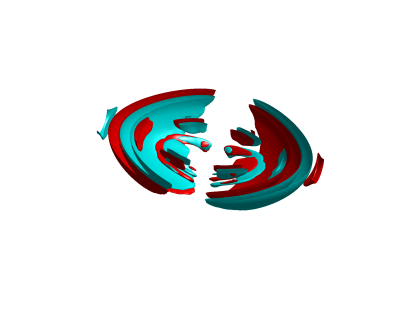
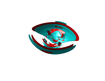
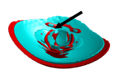
(A)	(B)	(C)

Figure 3: Snapshots of the contours for the particle velocity (A) $v_{1}$, (B) $v_{2}$, and (C) $v_{3}$ at $t=0.45s$. The black arrow in (C) indicates the shear wave front forming caustics.

6.3 Flat isotropic fluid-solid interface: Propagation of Scholte wave

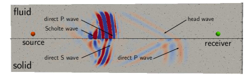
(a)

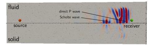
       (b)

Figure 4: Fluid-solid configuration visualized in the $x_{1}$–$x_{3}$ plane at $x_{2}=15.0$, with source and receiver located in the fluid. A snapshot at $t=12s$ is shown in (a), and a snapshot at $t=26s$ is shown in (b).

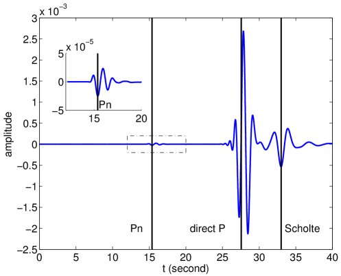
Figure 5: Seismic trace from a hydrophone located at $(40.0,\,15.0,\,6.0)$km in the fluid side. Arrival times of head wave Pn, direct P waves and Scholte waves are indicated by vertical lines.

We present a model with dimensions $[0,50]\times[0,30]\times[0,15]$km with a flat fluid-solid interface located at $x_{3}=7.5$km. The fluid side is homogeneous isotropic with an acoustic wave speed $1.5$km/s and density $1.0$g/cm${}^{\textrm{3}}$. The solid side is homogeneous isotropic with a P-wave speed $3.0$km/s and S-wave speed $1.5$km/s, and density $2.5$g/cm${}^{\textrm{3}}$. The Scholte wave speed is computed numerically as $1.2455$km/s [e.g., [Kaufman & Levshin(2005)]]. We place an explosive source in the fluid at location $(5.0,\,15.0,\,6.5)$km, using a Ricker wavelet as the source-time series with a central frequency of $2.0$Hz. A receiver is located at $(45.0,\,15.0,\,6.5)$km and records the synthetic phases for 40 seconds. We apply convolutional perfect matching layers (CPMLs)  [e.g., [Komatitsch & Martin(2007)]] for all external boundaries of the model, highlighting the effects of a fluid-solid internal boundary.

Two snapshots are shown in Figure 4, one for the solution at $t=12$s and the other for the solution at $t=26$s, in which we observe the occurence of a Scholte wave which is well seperated from the body wave phases at long times. The amplitude of the Scholte wave decays exponentially with the distance from fluid-solid interface [[Kaufman & Levshin(2005)]]. Figure 5 shows the seismogram as well as the arrival times of the head wave Pn, the direct P wave and Scholte wave. The modelled phase arrivals agree well with the travel times marked by perpendicular lines.

6.4 Seismic waves in a geological structure: SEAM model

In this application, the DG method’s ability to model the propagation and scattering of seismic waves in a field-scale domain with complex geological structures is demonstrated. The 3D SEAM (SEG Advanced Modeling) Phase I acoustic model is used that has heterogeneous structures and represents the sea-bed of the Gulf of Mexico [[Fehler & Keliher(2011)]]. It spans a 35 km by 40 km region of the earth’s surface and has a depth of 15 km, and is discretized as a regular grid with 20m $\times$ 20m $\times$ 10m sample interval. The model has several geological features that we will use to test the robustness of the DG method. It contains a high-velocity salt body that extends through the center of the model (Figure 6). The rapid contrast in velocity makes the model, in the language of partial differential equations, a stiff domain. Another geometric feature is the sedimentary layering at approximately 10 km under the surface. These layers will cause multiple scattering that will lead to constructive and destructive interference.

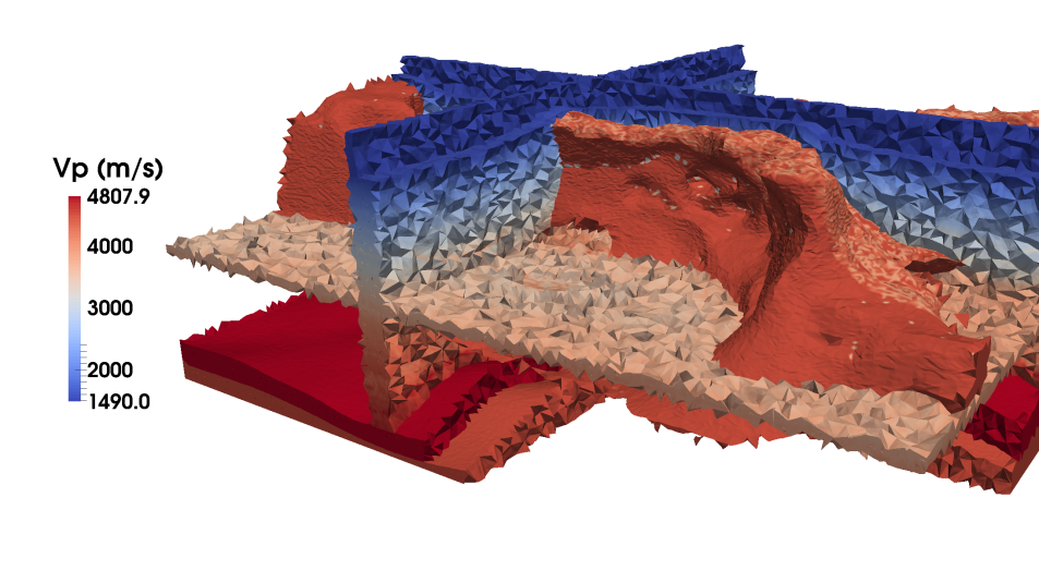
Figure 6: A tetrahedral meshing for the 3D SEAM generated by segmentation and mesh deformation techniques. The color map shows the P wavespeed $v_{p}$ interpolation.

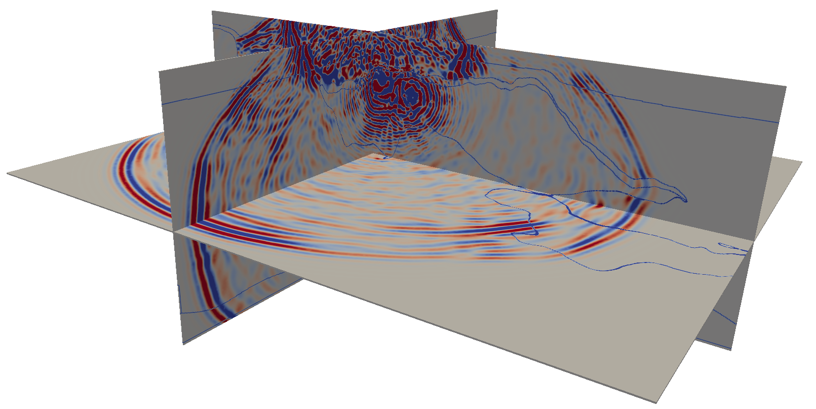
Figure 7: Slices of the 3D SEAM acoustic velocity model and snapshot of pressure wave field at $t=5.0$s, with the same viewpoint as in Figure 6.

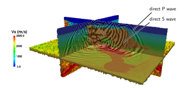
Figure 8: Slices of the isotropic extension of 3D SEAM Phase I shear wavespeed model and snapshot of 3-component of particle velocity at $t=5.0$s, with the same viewpoint as in Figure 6 and 7.

A tetrahedral mesh with 863,973 elements of order 3 is generated adaptively starting from the contours of the wave speed model, including the rough boundary of the salt body (Figure 6) and selected smooth interfaces associated with the sedimentary layers. We generate triangular isosurfaces based on domain partitioning of the wavespeed model into four primary subdomains: the ocean layer, the salt body, a high-contrast sediment layer and the sediment background. We also adaptively add vertices by tracking the contrasts of wavespeed inside each subregion. Using these, a tetrahedral mesh was created using TetGen [[Si(2015)]]. A point source is located at the ocean bottom $(x_{1},x_{2},x_{3})=(17.5,15.0,1.45)$km and the source function was a Ricker wavelet with a center frequency of 10.0 Hz. A snapshot of the acoustic pressure wave field solution is shown in Figure 7.

We also consider an extension of the SEAM Phase I model to isotropic elasiticity as is presented by [Oristaglio(2012)]. We represent, via interpolation, the S wave speed and density on the unstructured mesh based on the four distinct subdomains, and place a point source inside the ocean layer at $(x_{1},x_{2},x_{3})=(17.5,15.0,0.10)$km using a Ricker wavelet with a center frequency of 5.0 Hz. We apply a pressure-free surface boundary condition on the ocean surface, and CPMLs elsewhere. The S wavespeed and $3$-component of the particle velocity are shown in Figure 8, in which the shear wave front can be clearly observed after the P arrivals.

6.5 Scattering from a rough surface: Fractured carbonate

Here, we model the reflection generated by an explosive point source from a rough surface embedded in a transversely isotropic medium. This type of medium closely resembles fractured samples of carbonate rocks [[Li et al.(2009)Li, Petrovitch, & Pyrak-Nolte]]. Carbonates are abundantly found in nature. They pose many complications when working with them in the field because the physical properties vary from site to site and are strongly heterogeneous within the bulk rock. A homogeneous transversely isotropic medium can be used to model a carbonate because a variation in velocity amongst layers is the most common form of heterogeneity [[Nurmi et al.(1990)Nurmi, Charara, Waterhouse, & Park]].

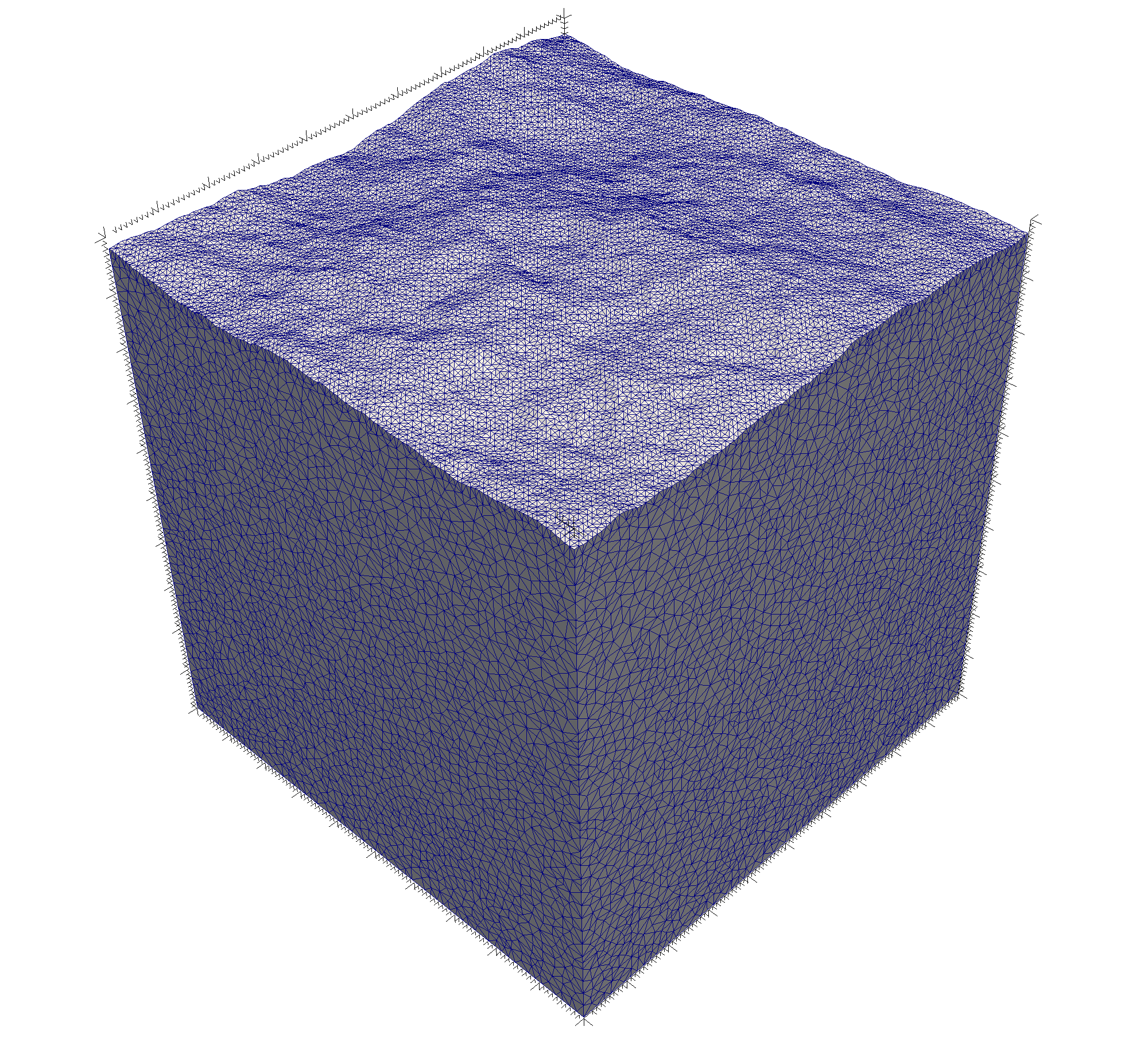
(A)	(B)

Figure 9: (A) Domain of the digitized rough surface. (B) Zoomed in of the mesh. The unit of the axises are in meters.

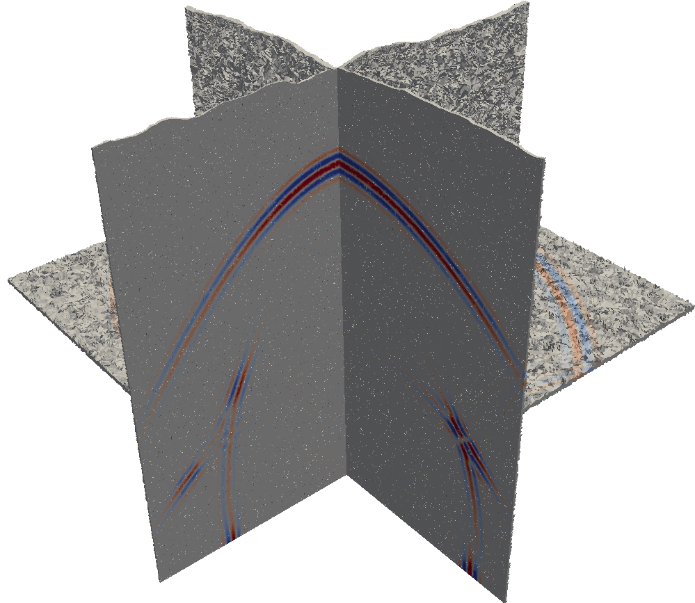
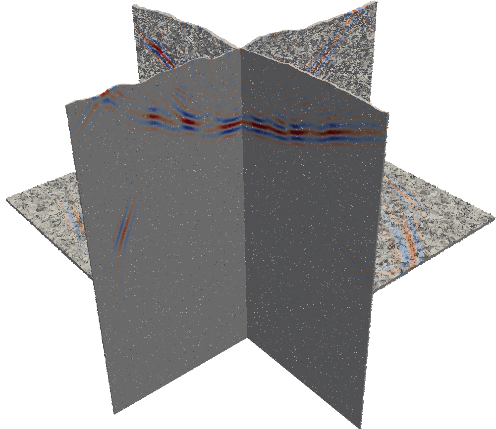
(A)	(B)
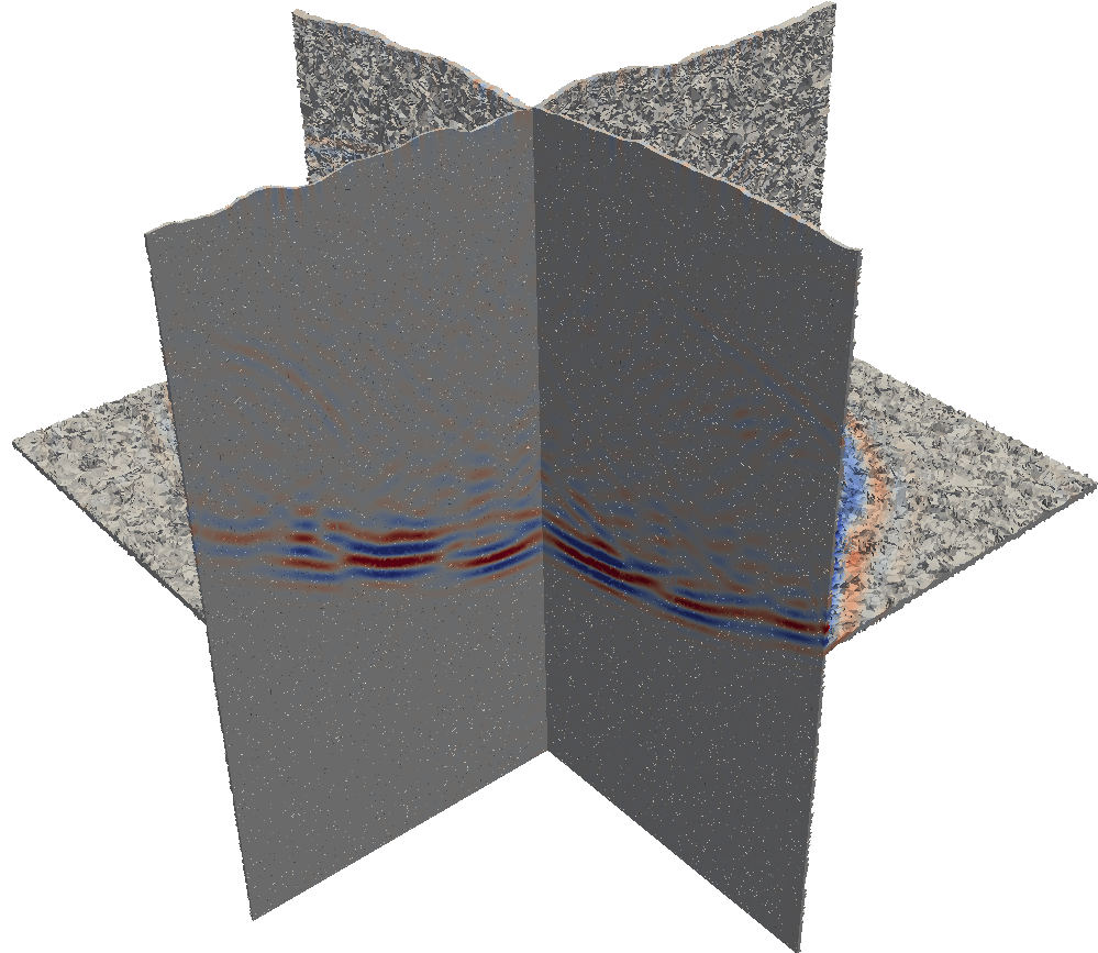
(C)

Figure 10: Slices of the $V_{3}$ wave field after (A) 21 $\mu s$, (B) 31 $\mu s$, and (C) 41 $\mu s$ from a 3D rough surface.

Laser profilometry was used to measure the surface roughness of an induced fracture in Austin Chalk, a carbonate rock sample. From these measurements, a profile of the surface was extracted to provide a rough boundary in an otherwise cubic domain with edge length of 0.1 m. The rough surface was placed on the top plane of the box, i.e. $x_{3}=0.1$m (Figure 9). The material properties were chosen such that the symmetry axis was in the $(\hat{x}_{1},\hat{x}_{2},\hat{x}_{3})=(0,1,0)$ direction. P- and S-phase velocities along the axis of symmetry are 4000 m/s and 2280 m/s respectively, and are 4900 m/s and 2000 m/s respectively along the other two directions. The following table provides a list of the specific elastic constants used:
$\rho$ $C_{11}$ $C_{22}$ $C_{33}$ $C_{44}$ $C_{55}$ $C_{66}$ $C_{23}$ $C_{13}$ $C_{12}$ 1.5 (g/cm${}^{\textrm{3}}$) 24.00 16.00 24.00 4.00 5.20 4.00 8.00 13.60 8.00 (GPa)
The tetrahedral mesh contains 686,444 elements, with $N_{p}=4$. We place an explosive source at $(x_{1},x_{2},x_{3})=(.05,.05,0)$, using a Ricker wavelet with a central frequency of 1 MHz. Two snapshots of the wave field were taken of the $3$-component of the particle velocity (Figure 10) that display the formation of shear-wave caustics due to anisotropy at $t=21\mu s$, and the solutions of scattering at $t=31\mu s$ and $t=41\mu s$, respectively.

6.6 Heterogeneous anisotropic solid-fluid boundary with topography

Here, we use our DG method to simulate the wave propagation and scattering in a heterogeneous anisotropic solid-fluid configuration. The solid-fluid boundary has topography, which is well described by adaptively fitting an unstructured mesh (see Figure 11(a)). The model has dimensions $[0,50]\times[0,30]\times[0,15]$km. The fluid side is homogeneous isotropic with an acoustic wave speed $1.5$km/s and density $1.0$g/cm${}^{\textrm{3}}$. The solid side consists of a reference HTI medium component with elastic parameters given by $C_{11}=33.75,\,C_{22}=22.50,\,C_{33}=13.85,\,C_{23}=13.85,\,C_{13}=11.44,\,C_{12}=11.44,\,C_{44}=4.327,\,C_{55}=5.625,\,C_{66}=5.625$ (GPa), and $\rho=2.5$g/cm${}^{\textrm{3}}$. A low-velocity lens is superimposed with its center located at $(25,\,15,\,9)$km. We place an explosive source in the fluid at location $(8.0,\,15.0,\,6.5)$km, using a Ricker wavelet as source-time series with a central frequency of $1.0$Hz. We apply convolutional perfect matching layers (CPMLs) for all external boundaries of the model with the thickness of approximately two central wavelengths.

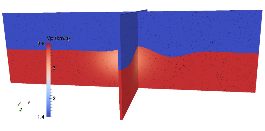
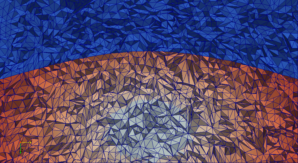
(a)

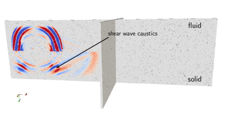
(b)

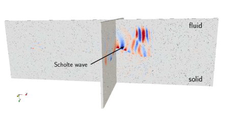
(c)

Figure 11: Heterogeneous HTI solid-fluid boundary with topography. (a) 3D model setting, with color indicating quasi-P wavespeed; (b) snapshot at t=4.0s; (c) snapshot at t=18.0s.

The waves are propagated for 40 seconds. Two snapshots in time of the wave field are shown; the solution at $t=4$s (Figure 11 (b)) and the solution at $t=14$s (Figure 11 (c)), with the occurence of a Scholte wave and seperation from body waves while propagating. We note the fomation of caustics in the solid region, caused by the anisotropy and the low-velocity lens.

7 Discussion

We develop a DG-method based numerical approach to simulate acousto-elastic wave phenomena. We demonstrate its ability to generate accurate solutions in domains with heterogeneous and complex geometries for long-time simulation. We briefly discuss the specifics of and differences between our and earlier developed DG methods for general acousto-elastic wave problems.

Most of the existing DG discretizations for solving the acousto-elastic system of equations in the first-order formulation make use of an upwind numerical flux derived from the elementwise solution of a Riemann problem. In [Dumbser & Käser(2006)], a Godunov upwind flux is applied upon diagonalizing the coefficient matrix in the stress-velocity formulation at element-element interfaces. Specifically, they use a “one-sided” upwind numerical flux and, to avoid elementwise numerical integration and make use of pre-calculated matrices instead, restrict the coefficients to be constant in each element. Steger-Warming flux-vector splitting in [Smith et al.(2010)Smith, Collis, Ober, Overfelt, & Schwaiger] is another way to obtain an exact Riemann solution for the linear system with flexibly parameterized isotropic elastic media, allowing variable coefficient within elements. The velocity-strain formulation introduced by [Wilcox et al.(2010)Wilcox, Stadler, Burstedde, & Ghattas] uses the Rankine-Hugoniot jump condition to obtain an upwind flux for isotropic solid-fluid interfaces while designing a uniform conservative formulation for coupled elasto-acoustic systems.

Meanwhile, there are penalty based DG schemes designed to solve numerically the second-order system of equations for the displacement. The interior penalty Galerkin method is used by [Rivière & Wheeler(2000)] to solve a nonlinear parabolic system, and a symmetric interior penalty term was employed by [Grote et al.(2006)Grote, Schneebeli, & Schötzau] to make the stiffness matrix symmetric positive definite. [De Basabe et al.(2008)De Basabe, Sen, & Wheeler] studies the dispersion and convergence of these interior penalty DG-method based schemes for the second-order elliptic Lamé system. [Warburton(2013)] defines for a general hyperbolic system a flux that penalizes the fields based on their continuity.

In our DG-method based scheme, we introduce a penalized numerical flux the form of which is motivated by the interior boundary continuity conditions. The fluid-solid boundary conditions are accounted for in the coupling of elements through the fluxes. Our penalty weight does not depend on the normal direction of the interior faces of the elements, and moreover, unlike the interior penalty scheme in the second-order displacement formulation, does not depend on the mesh size either.

8 Acknowledgment

This research was supported in part by the members, BGP, ExxonMobil, PGS, Statoil and Total, of the Geo-Mathematical Imaging Group.

Appendix A Convergence analysis

In this section we consider the $L^{2}$ error of numerical solutions $\textbf{\em q}_{h}$ and $\widetilde{\textbf{\em q}}_{h}$, which satisfy (31)–(32) for any $\textbf{\em p}_{h}$ and $\widetilde{\textbf{\em p}}_{h}\in V_{h}^{N_{p}}$. We denote by $\pi_{h}^{N_{p}}:L^{2}\mapsto V_{h}^{N_{p}}$ the $L^{2}$ projection onto the polynomial space of order $N_{p}$. We assume that $\textbf{\em f}-\textbf{\em f}_{h}=0$ and $\widetilde{f}-\widetilde{f}_{h}=0$, and no error occurs for $L^{2}$ projection of coefficient matrices, that is, $\mathcal{A}-\mathcal{A}_{h}=0,{\mathbfcal{Q}}-{\mathbfcal{Q}}_{h}=0$ and ${\Lambda}-{\Lambda}_{h}=0$. We define ${\textbf{\em e}}:=\textbf{\em q}-\textbf{\em q}_{h}$ and ${\widetilde{\textbf{\em e}}}:=\widetilde{\textbf{\em q}}-\widetilde{\textbf{\em q}}_{h}$, where q and $\widetilde{\textbf{\em q}}$ are the exact solutions. We also denote ${\boldsymbol{\eta}}:=\textbf{\em q}_{h}-\pi_{h}^{N_{p}}\textbf{\em q}\,,\,\,\widetilde{\boldsymbol{\eta}}:=\widetilde{\textbf{\em q}}_{h}-\pi_{h}^{N_{p}}\widetilde{\textbf{\em q}}\,$, and ${\boldsymbol{\epsilon}}:=(1-\pi_{h}^{N_{p}})\textbf{\em q}\,,\,\,\widetilde{\boldsymbol{\epsilon}}:=(1-\pi_{h}^{N_{p}})\widetilde{\textbf{\em q}}\,$; thus ${\textbf{\em e}}={\boldsymbol{\epsilon}}-{\boldsymbol{\eta}},\,{\widetilde{\textbf{\em e}}}=\widetilde{\boldsymbol{\epsilon}}-\widetilde{\boldsymbol{\eta}}$. We define the volume residuals

$$\mathrm{res}_{\scriptscriptstyle\mathrm{S}}(\textbf{\em q}_{h}):={\Lambda}^{T}\left({\mathbfcal{Q}}\frac{\partial\textbf{\em q}_{h}}{\partial t}-\nabla\cdot(\mathcal{A}\textbf{\em q}_{h})\right),\quad\widetilde{\mathrm{res}}_{\scriptscriptstyle\mathrm{F}}(\widetilde{\textbf{\em q}}_{h}):=\widetilde{{\Lambda}}^{T}\left(\widetilde{{\mathbfcal{Q}}}\frac{\partial\widetilde{\textbf{\em q}}_{h}}{\partial t}-\nabla\cdot(\widetilde{\mathcal{A}}\widetilde{\textbf{\em q}}_{h})\right),$$ (42)

and surface residuals

$$\begin{split}&\mathrm{res}_{\scriptscriptstyle\mathrm{SS}}(\textbf{\em q}_{h}):=\tfrac{1}{2}({\Lambda}^{-})^{T}{\,[\![\mathcal{A}_{n}\textbf{\em q}_{h}\,]\!]}_{\scriptscriptstyle\mathrm{SS}}+\alpha(\mathcal{A}_{n}^{-})^{T}{\,[\![\mathcal{A}_{n}\textbf{\em q}_{h}\,]\!]}_{\scriptscriptstyle\mathrm{SS}},\\ &\widetilde{\mathrm{res}}_{\scriptscriptstyle\mathrm{FS}}(\widetilde{\textbf{\em q}}_{h}):=\tfrac{1}{2}(\widetilde{{\Lambda}}^{-})^{T}{\,[\![\widetilde{\mathcal{A}}_{n}\widetilde{\textbf{\em q}}_{h}\,]\!]}_{\scriptscriptstyle\mathrm{FS}}+\alpha(\widetilde{\mathcal{A}}_{n}^{-})^{T}{\,[\![\widetilde{\mathcal{A}}_{n}\widetilde{\textbf{\em q}}_{h}\,]\!]}_{\scriptscriptstyle\mathrm{FS}},\\ &\mathrm{res}_{\scriptscriptstyle\mathrm{SF}}(\textbf{\em q}_{h}):=\tfrac{1}{2}({\Lambda}^{-})^{T}{\,[\![\mathcal{A}_{n}\textbf{\em q}_{h}\,]\!]}_{\scriptscriptstyle\mathrm{SF}}+\alpha(\mathcal{A}_{n}^{-})^{T}{\,[\![\mathcal{A}_{n}\textbf{\em q}_{h}\,]\!]}_{\scriptscriptstyle\mathrm{SF}},\\ &\widetilde{\mathrm{res}}_{\scriptscriptstyle\mathrm{FF}}(\widetilde{\textbf{\em q}}_{h}):=\tfrac{1}{2}(\widetilde{{\Lambda}}^{-})^{T}{\,[\![\widetilde{\mathcal{A}}_{n}\widetilde{\textbf{\em q}}_{h}\,]\!]}_{\scriptscriptstyle\mathrm{FF}}+\alpha(\widetilde{\mathcal{A}}_{n}^{-})^{T}{\,[\![\widetilde{\mathcal{A}}_{n}\widetilde{\textbf{\em q}}_{h}\,]\!]}_{\scriptscriptstyle\mathrm{FF}}.\end{split}$$ (43)

Using (31)–(32), it follows that $({\textbf{\em e}},{\widetilde{\textbf{\em e}}})$ satisfy

$$\begin{split}{\sum_{\mathrm{e}}}\int_{{D^{\mathrm{e}}_{\scriptscriptstyle\mathrm{S}}}}\mathrm{res}_{\scriptscriptstyle\mathrm{S}}({\textbf{\em e}})\cdot\textbf{\em p}_{h}\,\mathrm{d}\Omega-{\sum_{\mathrm{e}}}\int_{{\Sigma_{{\scriptscriptstyle\mathrm{SS}}}^{\mathrm{e}}}}\mathrm{res}_{\scriptscriptstyle\mathrm{SS}}({\textbf{\em e}})\cdot\textbf{\em p}_{h}^{-}\,\mathrm{d}\Sigma-{\sum_{\mathrm{e}}}\int_{{\Sigma_{{\scriptscriptstyle\mathrm{SF}}}^{\mathrm{e}}}}\mathrm{res}_{\scriptscriptstyle\mathrm{SF}}({\textbf{\em e}})\cdot\textbf{\em p}_{h}^{-}\,\mathrm{d}\Sigma=&0,\\ {\sum_{\mathrm{e}}}\int_{{D^{\mathrm{e}}_{\scriptscriptstyle\mathrm{F}}}}\widetilde{\mathrm{res}}_{\scriptscriptstyle\mathrm{F}}({\widetilde{\textbf{\em e}}})\cdot\widetilde{\textbf{\em p}}_{h}\,\mathrm{d}\Omega-{\sum_{\mathrm{e}}}\int_{{\Sigma_{{\scriptscriptstyle\mathrm{FS}}}^{\mathrm{e}}}}\widetilde{\mathrm{res}}_{\scriptscriptstyle\mathrm{FS}}({\widetilde{\textbf{\em e}}})\cdot\widetilde{\textbf{\em p}}_{h}^{-}\,\mathrm{d}\Sigma-{\sum_{\mathrm{e}}}\int_{{\Sigma_{{\scriptscriptstyle\mathrm{FF}}}^{\mathrm{e}}}}\widetilde{\mathrm{res}}_{\scriptscriptstyle\mathrm{FF}}({\widetilde{\textbf{\em e}}})\cdot\widetilde{\textbf{\em p}}_{h}^{-}\,\mathrm{d}\Sigma=&0,\end{split}$$ (44)

upon setting ${\mathbfcal{Q}}_{h}={\mathbfcal{Q}}$ and $\mathcal{A}_{h}=\mathcal{A}\,$. We take inner products of (42) and (43) with corresponding test functions, and immediately get, after summing up all the terms,

$$\begin{aligned} &{\sum_{\mathrm{e}}}\int_{{D^{\mathrm{e}}_{\scriptscriptstyle\mathrm{S}}}}{\mathbfcal{Q}}\frac{\partial\textbf{\em q}_{h}}{\partial t}\cdot{\Lambda}\textbf{\em p}_{h}\,\mathrm{d}\Omega-{\sum_{\mathrm{e}}}\int_{{D^{\mathrm{e}}_{\scriptscriptstyle\mathrm{S}}}}(\nabla\cdot(\mathcal{A}\textbf{\em q}_{h}))\cdot{\Lambda}\textbf{\em p}_{h}\,\mathrm{d}\Omega\\ &\hskip 28.45274pt-\tfrac{1}{2}{\sum_{\mathrm{e}}}\int_{{\Sigma_{{\scriptscriptstyle\mathrm{SS}}}^{\mathrm{e}}}}{\,[\![\mathcal{A}_{n}\textbf{\em q}_{h}\,]\!]}_{{\scriptscriptstyle\mathrm{SS}}}\cdot({\Lambda}\textbf{\em p}_{h})^{-}\,\mathrm{d}\Sigma-\tfrac{1}{2}{\sum_{\mathrm{e}}}\int_{{\Sigma_{{\scriptscriptstyle\mathrm{SF}}}^{\mathrm{e}}}}{\,[\![\mathcal{A}_{n}\textbf{\em q}_{h}\,]\!]}_{{\scriptscriptstyle\mathrm{SF}}}\cdot({\Lambda}\textbf{\em p}_{h})^{-}\,\mathrm{d}\Sigma\\ &\hskip 28.45274pt-\alpha{\sum_{\mathrm{e}}}\int_{{\Sigma_{{\scriptscriptstyle\mathrm{SS}}}^{\mathrm{e}}}}{\,[\![\mathcal{A}_{n}\textbf{\em q}_{h}\,]\!]}_{{\scriptscriptstyle\mathrm{SS}}}\cdot(\mathcal{A}_{n}\textbf{\em p}_{h})^{-}\,\mathrm{d}\Sigma-\alpha{\sum_{\mathrm{e}}}\int_{{\Sigma_{{\scriptscriptstyle\mathrm{SF}}}^{\mathrm{e}}}}{\,[\![\mathcal{A}_{n}\textbf{\em q}_{h}\,]\!]}_{{\scriptscriptstyle\mathrm{SF}}}\cdot(\mathcal{A}_{n}\textbf{\em p}_{h})^{-}\,\mathrm{d}\Sigma\\ =&{\sum_{\mathrm{e}}}\int_{{D^{\mathrm{e}}_{\scriptscriptstyle\mathrm{S}}}}\mathrm{res}_{\scriptscriptstyle\mathrm{S}}(\textbf{\em q}_{h})\cdot\textbf{\em p}_{h}\,\mathrm{d}\Omega-{\sum_{\mathrm{e}}}\int_{{\Sigma_{{\scriptscriptstyle\mathrm{SS}}}^{\mathrm{e}}}}\mathrm{res}_{\scriptscriptstyle\mathrm{SS}}(\textbf{\em q}_{h})\cdot\textbf{\em p}_{h}^{-}\,\mathrm{d}\Sigma-{\sum_{\mathrm{e}}}\int_{{\Sigma_{{\scriptscriptstyle\mathrm{SF}}}^{\mathrm{e}}}}\mathrm{res}_{\scriptscriptstyle\mathrm{SF}}(\textbf{\em q}_{h})\cdot\textbf{\em p}_{h}^{-}\,\mathrm{d}\Sigma,\\ \end{aligned}$$ (45)

$$\begin{aligned} &{\sum_{\mathrm{e}}}\int_{{D^{\mathrm{e}}_{\scriptscriptstyle\mathrm{F}}}}\widetilde{{\mathbfcal{Q}}}\frac{\partial\widetilde{\textbf{\em q}}_{h}}{\partial t}\cdot\widetilde{{\Lambda}}\widetilde{\textbf{\em p}}_{h}\,\mathrm{d}\Omega-{\sum_{\mathrm{e}}}\int_{{D^{\mathrm{e}}_{\scriptscriptstyle\mathrm{F}}}}(\nabla\cdot(\widetilde{\mathcal{A}}\widetilde{\textbf{\em q}}_{h}))\cdot\widetilde{{\Lambda}}\widetilde{\textbf{\em p}}_{h}\,\mathrm{d}\Omega\\ &\hskip 28.45274pt-\tfrac{1}{2}{\sum_{\mathrm{e}}}\int_{{\Sigma_{{\scriptscriptstyle\mathrm{FF}}}^{\mathrm{e}}}}{\,[\![\widetilde{\mathcal{A}}_{n}\widetilde{\textbf{\em q}}_{h}\,]\!]}_{{\scriptscriptstyle\mathrm{FF}}}\cdot(\widetilde{{\Lambda}}\widetilde{\textbf{\em p}}_{h})^{-}\,\mathrm{d}\Sigma-\tfrac{1}{2}{\sum_{\mathrm{e}}}\int_{{\Sigma_{{\scriptscriptstyle\mathrm{FS}}}^{\mathrm{e}}}}{\,[\![\widetilde{\mathcal{A}}_{n}\widetilde{\textbf{\em q}}_{h}\,]\!]}_{{\scriptscriptstyle\mathrm{FS}}}\cdot(\widetilde{{\Lambda}}\widetilde{\textbf{\em p}}_{h})^{-}\,\mathrm{d}\Sigma\\ &\hskip 28.45274pt-\alpha{\sum_{\mathrm{e}}}\int_{{\Sigma_{{\scriptscriptstyle\mathrm{FF}}}^{\mathrm{e}}}}{\,[\![\widetilde{\mathcal{A}}_{n}\widetilde{\textbf{\em q}}_{h}\,]\!]}_{{\scriptscriptstyle\mathrm{FF}}}\cdot(\widetilde{\mathcal{A}}_{n}\widetilde{\textbf{\em p}}_{h})^{-}\,\mathrm{d}\Sigma-\alpha{\sum_{\mathrm{e}}}\int_{{\Sigma_{{\scriptscriptstyle\mathrm{FS}}}^{\mathrm{e}}}}{\,[\![\widetilde{\mathcal{A}}_{n}\widetilde{\textbf{\em q}}_{h}\,]\!]}_{{\scriptscriptstyle\mathrm{FS}}}\cdot(\widetilde{\mathcal{A}}_{n}\widetilde{\textbf{\em p}}_{h})^{-}\,\mathrm{d}\Sigma\\ =&{\sum_{\mathrm{e}}}\int_{{D^{\mathrm{e}}_{\scriptscriptstyle\mathrm{F}}}}\widetilde{\mathrm{res}}_{\scriptscriptstyle\mathrm{F}}(\widetilde{\textbf{\em q}}_{h})\cdot\widetilde{\textbf{\em p}}_{h}\,\mathrm{d}\Omega-{\sum_{\mathrm{e}}}\int_{{\Sigma_{{\scriptscriptstyle\mathrm{FF}}}^{\mathrm{e}}}}\widetilde{\mathrm{res}}_{\scriptscriptstyle\mathrm{FF}}(\widetilde{\textbf{\em q}}_{h})\cdot\widetilde{\textbf{\em p}}_{h}^{-}\,\mathrm{d}\Sigma-{\sum_{\mathrm{e}}}\int_{{\Sigma_{{\scriptscriptstyle\mathrm{FS}}}^{\mathrm{e}}}}\widetilde{\mathrm{res}}_{\scriptscriptstyle\mathrm{FS}}(\widetilde{\textbf{\em q}}_{h})\cdot\widetilde{\textbf{\em p}}_{h}^{-}\,\mathrm{d}\Sigma.\\ \end{aligned}$$ (46)

We let $\textbf{\em q}_{h}=\textbf{\em p}_{h}={\boldsymbol{\eta}}$, $\widetilde{\textbf{\em q}}_{h}=\widetilde{\textbf{\em p}}_{h}=\widetilde{\boldsymbol{\eta}}$, when equations (45) and (LABEL:eq:numerical_residual_acoustic) become

$$\begin{aligned} &\frac{1}{2}\frac{\,\mathrm{d}}{\,\mathrm{d}t}{\sum_{\mathrm{e}}}{\|{\boldsymbol{\eta}}\,\|}_{L^{2}({D^{\mathrm{e}}_{\scriptscriptstyle\mathrm{S}}})}^{2}-\alpha{\sum_{\mathrm{e}}}\int_{{\Sigma_{{\scriptscriptstyle\mathrm{SS}}}^{\mathrm{e}}}}{\,[\![\mathcal{A}_{n}{\boldsymbol{\eta}}\,]\!]}_{{\scriptscriptstyle\mathrm{SS}}}\cdot(\mathcal{A}_{n}{\boldsymbol{\eta}})^{-}\,\mathrm{d}\Sigma-\alpha{\sum_{\mathrm{e}}}\int_{{\Sigma_{{\scriptscriptstyle\mathrm{SF}}}^{\mathrm{e}}}}{\,[\![\mathcal{A}_{n}{\boldsymbol{\eta}}\,]\!]}_{{\scriptscriptstyle\mathrm{SF}}}\cdot(\mathcal{A}_{n}{\boldsymbol{\eta}})^{-}\,\mathrm{d}\Sigma\\[-5.69054pt] &\hskip 14.22636pt-\left({\sum_{\mathrm{e}}}\int_{{D^{\mathrm{e}}_{\scriptscriptstyle\mathrm{S}}}}(\nabla\cdot(\mathcal{A}{\boldsymbol{\eta}}))\cdot{\Lambda}{\boldsymbol{\eta}}\,\mathrm{d}\Omega+\tfrac{1}{2}{\sum_{\mathrm{e}}}\int_{{\Sigma_{{\scriptscriptstyle\mathrm{SS}}}^{\mathrm{e}}}}{\,[\![\mathcal{A}_{n}{\boldsymbol{\eta}}\,]\!]}_{{\scriptscriptstyle\mathrm{SS}}}\cdot({\Lambda}{\boldsymbol{\eta}})^{-}\,\mathrm{d}\Sigma\right.\\[-11.38109pt] &\hskip 227.62204pt\left.+\tfrac{1}{2}{\sum_{\mathrm{e}}}\int_{{\Sigma_{{\scriptscriptstyle\mathrm{SF}}}^{\mathrm{e}}}}{\,[\![\mathcal{A}_{n}{\boldsymbol{\eta}}\,]\!]}_{{\scriptscriptstyle\mathrm{SF}}}\cdot({\Lambda}{\boldsymbol{\eta}})^{-}\,\mathrm{d}\Sigma\right)\\ &={\sum_{\mathrm{e}}}\int_{{D^{\mathrm{e}}_{\scriptscriptstyle\mathrm{S}}}}\mathrm{res}_{\scriptscriptstyle\mathrm{S}}({\boldsymbol{\eta}})\cdot{\boldsymbol{\eta}}\,\mathrm{d}\Omega-{\sum_{\mathrm{e}}}\int_{{\Sigma_{{\scriptscriptstyle\mathrm{SS}}}^{\mathrm{e}}}}\mathrm{res}_{\scriptscriptstyle\mathrm{SS}}({\boldsymbol{\eta}})\cdot{\boldsymbol{\eta}}^{-}\,\mathrm{d}\Sigma-{\sum_{\mathrm{e}}}\int_{{\Sigma_{{\scriptscriptstyle\mathrm{SF}}}^{\mathrm{e}}}}\mathrm{res}_{\scriptscriptstyle\mathrm{SF}}({\boldsymbol{\eta}})\cdot{\boldsymbol{\eta}}^{-}\,\mathrm{d}\Sigma,\end{aligned}$$ (47)

$$\begin{aligned} &\frac{1}{2}\frac{\,\mathrm{d}}{\,\mathrm{d}t}{\sum_{\mathrm{e}}}{\|\widetilde{\boldsymbol{\eta}}\,\|}_{L^{2}({D^{\mathrm{e}}_{\scriptscriptstyle\mathrm{F}}})}^{2}-\alpha{\sum_{\mathrm{e}}}\int_{{\Sigma_{{\scriptscriptstyle\mathrm{FF}}}^{\mathrm{e}}}}{\,[\![\widetilde{\mathcal{A}}_{n}\widetilde{\boldsymbol{\eta}}\,]\!]}_{{\scriptscriptstyle\mathrm{FF}}}\cdot(\widetilde{\mathcal{A}}_{n}\widetilde{\boldsymbol{\eta}})^{-}\,\mathrm{d}\Sigma-\alpha{\sum_{\mathrm{e}}}\int_{{\Sigma_{{\scriptscriptstyle\mathrm{FS}}}^{\mathrm{e}}}}{\,[\![\widetilde{\mathcal{A}}_{n}\widetilde{\boldsymbol{\eta}}\,]\!]}_{{\scriptscriptstyle\mathrm{FS}}}\cdot(\widetilde{\mathcal{A}}_{n}\widetilde{\boldsymbol{\eta}})^{-}\,\mathrm{d}\Sigma\\[-5.69054pt] &\hskip 14.22636pt-\left({\sum_{\mathrm{e}}}\int_{D^{\mathrm{e}}_{\scriptscriptstyle\mathrm{F}}}(\nabla\cdot(\widetilde{\mathcal{A}}\widetilde{\boldsymbol{\eta}}))\cdot\widetilde{{\Lambda}}\widetilde{\boldsymbol{\eta}}\,\mathrm{d}\Omega+\tfrac{1}{2}{\sum_{\mathrm{e}}}\int_{{\Sigma_{{\scriptscriptstyle\mathrm{FF}}}^{\mathrm{e}}}}{\,[\![\widetilde{\mathcal{A}}_{n}\widetilde{\boldsymbol{\eta}}\,]\!]}_{{\scriptscriptstyle\mathrm{FF}}}\cdot(\widetilde{{\Lambda}}\widetilde{\boldsymbol{\eta}})^{-}\,\mathrm{d}\Sigma\right.\\[-11.38109pt] &\hskip 227.62204pt\left.+\tfrac{1}{2}{\sum_{\mathrm{e}}}\int_{{\Sigma_{{\scriptscriptstyle\mathrm{FS}}}^{\mathrm{e}}}}{\,[\![\widetilde{\mathcal{A}}_{n}\widetilde{\boldsymbol{\eta}}\,]\!]}_{{\scriptscriptstyle\mathrm{FS}}}\cdot(\widetilde{{\Lambda}}\widetilde{\boldsymbol{\eta}})^{-}\,\mathrm{d}\Sigma\right)\\ &={\sum_{\mathrm{e}}}\int_{D^{\mathrm{e}}_{\scriptscriptstyle\mathrm{F}}}\widetilde{\mathrm{res}}_{\scriptscriptstyle\mathrm{F}}(\widetilde{\boldsymbol{\eta}})\cdot\widetilde{\boldsymbol{\eta}}\,\mathrm{d}\Omega-{\sum_{\mathrm{e}}}\int_{{\Sigma_{{\scriptscriptstyle\mathrm{FF}}}^{\mathrm{e}}}}\widetilde{\mathrm{res}}_{\scriptscriptstyle\mathrm{FF}}(\widetilde{\boldsymbol{\eta}})\cdot\widetilde{\boldsymbol{\eta}}^{-}\,\mathrm{d}\Sigma-{\sum_{\mathrm{e}}}\int_{{\Sigma_{{\scriptscriptstyle\mathrm{FS}}}^{\mathrm{e}}}}\widetilde{\mathrm{res}}_{\scriptscriptstyle\mathrm{FS}}(\widetilde{\boldsymbol{\eta}})\cdot\widetilde{\boldsymbol{\eta}}^{-}\,\mathrm{d}\Sigma.\end{aligned}$$ (48)

Adding (47) and (48), and using the energy result in Section 4, the terms in between parentheses on the left-hand sides of both equations cancel one another, and the penalty terms turn into quadratic forms, that is,

$$\begin{split}&\frac{1}{2}\frac{\,\mathrm{d}}{\,\mathrm{d}t}\left({\sum_{\mathrm{e}}}{\|{\boldsymbol{\eta}}\,\|}\phantom{|}_{L^{2}({D^{\mathrm{e}}_{\scriptscriptstyle\mathrm{S}}};\,{\mathbfcal{Q}},{\Lambda})}^{2}+{\sum_{\mathrm{e}}}{\|\widetilde{\boldsymbol{\eta}}\,\|}\phantom{|}_{L^{2}({D^{\mathrm{e}}_{\scriptscriptstyle\mathrm{F}}};\,\widetilde{{\mathbfcal{Q}}},\widetilde{{\Lambda}})}^{2}\right)\\[-5.69054pt] &\hskip 5.69054pt+\frac{\alpha}{2}\left({\sum_{\mathrm{e}}}{\|{\,[\![\mathcal{A}_{n}{\boldsymbol{\eta}}\,]\!]}_{{\scriptscriptstyle\mathrm{SS}}}\,\|}_{L^{2}({\Sigma_{{\scriptscriptstyle\mathrm{SS}}}^{\mathrm{e}}})}^{2}+{\sum_{\mathrm{e}}}{\|{\,[\![\widetilde{\mathcal{A}}_{n}\widetilde{\boldsymbol{\eta}}\,]\!]}_{{\scriptscriptstyle\mathrm{FF}}}\,\|}_{L^{2}({\Sigma_{{\scriptscriptstyle\mathrm{FF}}}^{\mathrm{e}}})}^{2}+2{\sum_{\mathrm{e}}}{\|{\,[\![\mathcal{A}_{n}{\boldsymbol{\eta}}\,]\!]}_{{\scriptscriptstyle\mathrm{SF}}}\,\|}_{L^{2}({\Sigma_{{\scriptscriptstyle\mathrm{SF}}}^{\mathrm{e}}})}^{2}\right)\\ &={\sum_{\mathrm{e}}}\int_{{D^{\mathrm{e}}_{\scriptscriptstyle\mathrm{S}}}}\mathrm{res}_{\scriptscriptstyle\mathrm{S}}({\boldsymbol{\eta}})\cdot{\boldsymbol{\eta}}\,\mathrm{d}\Omega-{\sum_{\mathrm{e}}}\int_{{\Sigma_{{\scriptscriptstyle\mathrm{SS}}}^{\mathrm{e}}}}\mathrm{res}_{\scriptscriptstyle\mathrm{SS}}({\boldsymbol{\eta}})\cdot{\boldsymbol{\eta}}^{-}\,\mathrm{d}\Sigma-{\sum_{\mathrm{e}}}\int_{{\Sigma_{{\scriptscriptstyle\mathrm{SF}}}^{\mathrm{e}}}}\mathrm{res}_{\scriptscriptstyle\mathrm{SF}}({\boldsymbol{\eta}})\cdot{\boldsymbol{\eta}}^{-}\,\mathrm{d}\Sigma\\[-5.69054pt] &\hskip 5.69054pt+{\sum_{\mathrm{e}}}\int_{{D^{\mathrm{e}}_{\scriptscriptstyle\mathrm{F}}}}\widetilde{\mathrm{res}}_{\scriptscriptstyle\mathrm{F}}(\widetilde{\boldsymbol{\eta}})\cdot\widetilde{\boldsymbol{\eta}}\,\mathrm{d}\Omega-{\sum_{\mathrm{e}}}\int_{{\Sigma_{{\scriptscriptstyle\mathrm{FF}}}^{\mathrm{e}}}}\widetilde{\mathrm{res}}_{\scriptscriptstyle\mathrm{FF}}(\widetilde{\boldsymbol{\eta}})\cdot\widetilde{\boldsymbol{\eta}}^{-}\,\mathrm{d}\Sigma-{\sum_{\mathrm{e}}}\int_{{\Sigma_{{\scriptscriptstyle\mathrm{FS}}}^{\mathrm{e}}}}\widetilde{\mathrm{res}}_{\scriptscriptstyle\mathrm{FS}}(\widetilde{\boldsymbol{\eta}})\cdot\widetilde{\boldsymbol{\eta}}^{-}\,\mathrm{d}\Sigma.\end{split}$$ (49)

Let $\textbf{\em p}_{h}={\boldsymbol{\eta}}$ in (44), and subtract it from the right-hand side of (49). We note that ${\textbf{\em e}}={\boldsymbol{\epsilon}}-{\boldsymbol{\eta}},\,{\widetilde{\textbf{\em e}}}=\widetilde{\boldsymbol{\epsilon}}-\widetilde{\boldsymbol{\eta}}$, and obtain

$$\begin{split}&\frac{1}{2}\frac{\,\mathrm{d}}{\,\mathrm{d}t}\left({\sum_{\mathrm{e}}}{\|{\boldsymbol{\eta}}\,\|}\phantom{|}_{L^{2}({D^{\mathrm{e}}_{\scriptscriptstyle\mathrm{S}}};\,{\mathbfcal{Q}},{\Lambda})}^{2}+{\sum_{\mathrm{e}}}{\|\widetilde{\boldsymbol{\eta}}\,\|}\phantom{|}_{L^{2}({D^{\mathrm{e}}_{\scriptscriptstyle\mathrm{F}}};\,\widetilde{{\mathbfcal{Q}}},\widetilde{{\Lambda}})}^{2}\right)\\[-2.84526pt] &\hskip 5.69054pt+\frac{\alpha}{2}\left({\sum_{\mathrm{e}}}{\|{\,[\![\mathcal{A}_{n}{\boldsymbol{\eta}}\,]\!]}_{{\scriptscriptstyle\mathrm{SS}}}\,\|}_{L^{2}({\Sigma_{{\scriptscriptstyle\mathrm{SS}}}^{\mathrm{e}}})}^{2}+{\sum_{\mathrm{e}}}{\|{\,[\![\widetilde{\mathcal{A}}_{n}\widetilde{\boldsymbol{\eta}}\,]\!]}_{{\scriptscriptstyle\mathrm{FF}}}\,\|}_{L^{2}({\Sigma_{{\scriptscriptstyle\mathrm{FF}}}^{\mathrm{e}}})}^{2}+2{\sum_{\mathrm{e}}}{\|{\,[\![\mathcal{A}_{n}{\boldsymbol{\eta}}\,]\!]}_{{\scriptscriptstyle\mathrm{SF}}}\,\|}_{L^{2}({\Sigma_{{\scriptscriptstyle\mathrm{SF}}}^{\mathrm{e}}})}^{2}\right)\\ &={\sum_{\mathrm{e}}}\int_{{D^{\mathrm{e}}_{\scriptscriptstyle\mathrm{S}}}}\mathrm{res}_{\scriptscriptstyle\mathrm{S}}({\boldsymbol{\epsilon}})\cdot{\boldsymbol{\eta}}\,\mathrm{d}\Omega-{\sum_{\mathrm{e}}}\int_{{\Sigma_{{\scriptscriptstyle\mathrm{SS}}}^{\mathrm{e}}}}\mathrm{res}_{\scriptscriptstyle\mathrm{SS}}({\boldsymbol{\epsilon}})\cdot{\boldsymbol{\eta}}^{-}\,\mathrm{d}\Sigma-{\sum_{\mathrm{e}}}\int_{{\Sigma_{{\scriptscriptstyle\mathrm{SF}}}^{\mathrm{e}}}}\mathrm{res}_{\scriptscriptstyle\mathrm{SF}}({\boldsymbol{\epsilon}})\cdot{\boldsymbol{\eta}}^{-}\,\mathrm{d}\Sigma\\[-5.69054pt] &\hskip 5.69054pt+{\sum_{\mathrm{e}}}\int_{{D^{\mathrm{e}}_{\scriptscriptstyle\mathrm{F}}}}\widetilde{\mathrm{res}}_{\scriptscriptstyle\mathrm{F}}(\widetilde{\boldsymbol{\epsilon}})\cdot\widetilde{\boldsymbol{\eta}}\,\mathrm{d}\Omega-{\sum_{\mathrm{e}}}\int_{{\Sigma_{{\scriptscriptstyle\mathrm{FF}}}^{\mathrm{e}}}}\widetilde{\mathrm{res}}_{\scriptscriptstyle\mathrm{FF}}(\widetilde{\boldsymbol{\epsilon}})\cdot\widetilde{\boldsymbol{\eta}}^{-}\,\mathrm{d}\Sigma-{\sum_{\mathrm{e}}}\int_{{\Sigma_{{\scriptscriptstyle\mathrm{FS}}}^{\mathrm{e}}}}\widetilde{\mathrm{res}}_{\scriptscriptstyle\mathrm{FS}}(\widetilde{\boldsymbol{\epsilon}})\cdot\widetilde{\boldsymbol{\eta}}^{-}\,\mathrm{d}\Sigma.\end{split}$$ (50)

Having the energy result (50), which corresponds with Equation (5.10) in [Warburton(2013)], we follow the same process as described in the reference.

We apply integration by parts:

$$\begin{split}&\int_{D^{\mathrm{e}}_{\scriptscriptstyle\mathrm{S}}}(\nabla\cdot(\mathcal{A}\textbf{\em q}))\cdot({\Lambda}\textbf{\em p})\,\mathrm{d}\Omega=\int_{D^{\mathrm{e}}_{\scriptscriptstyle\mathrm{S}}}(\nabla\cdot{(\textbf{\em C}\textbf{\em E}\,)})\cdot\textbf{\em w}+\tfrac{1}{2}(\nabla\textbf{\em v}+\nabla\textbf{\em v}^{T}):(\textbf{\em C}\textbf{\em H})\,\mathrm{d}\Omega\\ &\hskip 28.45274pt=-\int_{D^{\mathrm{e}}_{\scriptscriptstyle\mathrm{S}}}{(\textbf{\em C}\textbf{\em E}\,)}:\tfrac{1}{2}(\nabla\textbf{\em w}+\nabla\textbf{\em w}^{T})+\textbf{\em v}\cdot(\nabla\cdot(\textbf{\em C}\textbf{\em H}))\,\mathrm{d}\Omega\\[-8.53581pt] &\hskip 68.28644pt+\int_{{\Sigma_{{\scriptscriptstyle\mathrm{SS}}}^{\mathrm{e}}}\cup{\Sigma_{{\scriptscriptstyle\mathrm{SF}}}^{\mathrm{e}}}}(\textbf{\em n}\cdot{(\textbf{\em C}\textbf{\em E}\,)})^{-}\cdot\textbf{\em w}^{-}+\textbf{\em v}^{-}\cdot(\textbf{\em n}\cdot(\textbf{\em C}\textbf{\em H}))^{-}\,\mathrm{d}\Sigma\\ &\hskip 28.45274pt=\boxed{-\int_{D^{\mathrm{e}}_{\scriptscriptstyle\mathrm{S}}}(\nabla\cdot(\mathcal{A}\textbf{\em p}))\cdot({\Lambda}\textbf{\em q})\,\mathrm{d}\Omega}+\int_{{\Sigma_{{\scriptscriptstyle\mathrm{SS}}}^{\mathrm{e}}}\cup{\Sigma_{{\scriptscriptstyle\mathrm{SF}}}^{\mathrm{e}}}}(\mathcal{A}_{n}\textbf{\em q})^{-}\cdot({\Lambda}\textbf{\em p})^{-}\,\mathrm{d}\Sigma,\end{split}$$ (51)

and similarly

$$\int_{D^{\mathrm{e}}_{\scriptscriptstyle\mathrm{F}}}(\nabla\cdot(\widetilde{\mathcal{A}}\widetilde{\textbf{\em q}}))\cdot(\widetilde{{\Lambda}}\widetilde{\textbf{\em p}})\,\mathrm{d}\Omega=\boxed{-\int_{D^{\mathrm{e}}_{\scriptscriptstyle\mathrm{F}}}(\nabla\cdot(\widetilde{\mathcal{A}}\widetilde{\textbf{\em p}}))\cdot(\widetilde{{\Lambda}}\textbf{\em q})\,\mathrm{d}\Omega}+\int_{{\Sigma_{{\scriptscriptstyle\mathrm{FS}}}^{\mathrm{e}}}\cup{\Sigma_{{\scriptscriptstyle\mathrm{FF}}}^{\mathrm{e}}}}(\widetilde{\mathcal{A}}_{n}\widetilde{\textbf{\em q}})^{-}\cdot(\widetilde{{\Lambda}}\widetilde{\textbf{\em p}})^{-}\,\mathrm{d}\Sigma.$$ (52)

We set $\textbf{\em q}={\boldsymbol{\epsilon}},\,\textbf{\em p}={\boldsymbol{\eta}}$ in (51) and $\widetilde{\textbf{\em q}}=\widetilde{\boldsymbol{\epsilon}},\,\widetilde{\textbf{\em p}}=\widetilde{\boldsymbol{\eta}}$ in (52). The boxed terms in (51) and (52) vanish as the projection errors ${\boldsymbol{\epsilon}}$ and $\widetilde{\boldsymbol{\epsilon}}$ are orthogonal to the spatial derivatives of the polynomial solutions $\textbf{\em q}_{h}$ and $\widetilde{\textbf{\em q}}_{h}$ by Galerkin approximation, and then the right-hand side of (50) becomes

$$\begin{aligned} &{\sum_{\mathrm{e}}}\int_{{D^{\mathrm{e}}_{\scriptscriptstyle\mathrm{S}}}}\mathrm{res}_{\scriptscriptstyle\mathrm{S}}({\boldsymbol{\epsilon}})\cdot{\boldsymbol{\eta}}\,\mathrm{d}\Omega-{\sum_{\mathrm{e}}}\int_{{\Sigma_{{\scriptscriptstyle\mathrm{SS}}}^{\mathrm{e}}}}\mathrm{res}_{\scriptscriptstyle\mathrm{SS}}({\boldsymbol{\epsilon}})\cdot{\boldsymbol{\eta}}^{-}\,\mathrm{d}\Sigma-{\sum_{\mathrm{e}}}\int_{{\Sigma_{{\scriptscriptstyle\mathrm{SF}}}^{\mathrm{e}}}}\mathrm{res}_{\scriptscriptstyle\mathrm{SF}}({\boldsymbol{\epsilon}})\cdot{\boldsymbol{\eta}}^{-}\,\mathrm{d}\Sigma\\[-5.69054pt] &\hskip 5.69054pt+{\sum_{\mathrm{e}}}\int_{{D^{\mathrm{e}}_{\scriptscriptstyle\mathrm{F}}}}\widetilde{\mathrm{res}}_{\scriptscriptstyle\mathrm{F}}(\widetilde{\boldsymbol{\epsilon}})\cdot\widetilde{\boldsymbol{\eta}}\,\mathrm{d}\Omega-{\sum_{\mathrm{e}}}\int_{{\Sigma_{{\scriptscriptstyle\mathrm{FF}}}^{\mathrm{e}}}}\widetilde{\mathrm{res}}_{\scriptscriptstyle\mathrm{FF}}(\widetilde{\boldsymbol{\epsilon}})\cdot\widetilde{\boldsymbol{\eta}}^{-}\,\mathrm{d}\Sigma-{\sum_{\mathrm{e}}}\int_{{\Sigma_{{\scriptscriptstyle\mathrm{FS}}}^{\mathrm{e}}}}\widetilde{\mathrm{res}}_{\scriptscriptstyle\mathrm{FS}}(\widetilde{\boldsymbol{\epsilon}})\cdot\widetilde{\boldsymbol{\eta}}^{-}\,\mathrm{d}\Sigma\end{aligned}$$

$$\hskip 14.22636pt\boxed{=\hskip 11.38109pt{\sum_{\mathrm{e}}}\int_{{D^{\mathrm{e}}_{\scriptscriptstyle\mathrm{S}}}}{\mathbfcal{Q}}\frac{\partial{\boldsymbol{\epsilon}}}{\partial t}\cdot({\Lambda}{\boldsymbol{\eta}})\,\mathrm{d}\Omega+{\sum_{\mathrm{e}}}\int_{{D^{\mathrm{e}}_{\scriptscriptstyle\mathrm{F}}}}\widetilde{{\mathbfcal{Q}}}\frac{\partial\widetilde{\boldsymbol{\epsilon}}}{\partial t}\cdot(\widetilde{{\Lambda}}\widetilde{\boldsymbol{\eta}})\,\mathrm{d}\Omega} \Xi_{1}$$ ()

$$\hskip 14.22636pt\boxed{\begin{aligned} &-{\sum_{\mathrm{e}}}\int_{{\Sigma_{{\scriptscriptstyle\mathrm{SS}}}^{\mathrm{e}}}}\{\!\{\mathcal{A}_{n}{\boldsymbol{\epsilon}}\,\}\!\}_{\scriptscriptstyle\mathrm{SS}}\cdot({\Lambda}{\boldsymbol{\eta}})^{-}\,\mathrm{d}\Sigma-{\sum_{\mathrm{e}}}\int_{{\Sigma_{{\scriptscriptstyle\mathrm{SF}}}^{\mathrm{e}}}}\{\!\{\mathcal{A}_{n}{\boldsymbol{\epsilon}}\,\}\!\}_{\scriptscriptstyle\mathrm{SF}}\cdot({\Lambda}{\boldsymbol{\eta}})^{-}\,\mathrm{d}\Sigma\\ &-{\sum_{\mathrm{e}}}\int_{{\Sigma_{{\scriptscriptstyle\mathrm{FF}}}^{\mathrm{e}}}}\{\!\{\widetilde{\mathcal{A}}_{n}\widetilde{\boldsymbol{\epsilon}}\,\}\!\}_{\scriptscriptstyle\mathrm{FF}}\cdot(\widetilde{{\Lambda}}\widetilde{\boldsymbol{\eta}})^{-}\,\mathrm{d}\Sigma-{\sum_{\mathrm{e}}}\int_{{\Sigma_{{\scriptscriptstyle\mathrm{FS}}}^{\mathrm{e}}}}\{\!\{\widetilde{\mathcal{A}}_{n}\widetilde{\boldsymbol{\epsilon}}\,\}\!\}_{\scriptscriptstyle\mathrm{FS}}\cdot(\widetilde{{\Lambda}}\widetilde{\boldsymbol{\eta}})^{-}\,\mathrm{d}\Sigma\\ &-\alpha{\sum_{\mathrm{e}}}\int_{{\Sigma_{{\scriptscriptstyle\mathrm{SS}}}^{\mathrm{e}}}}{\,[\![\mathcal{A}_{n}{\boldsymbol{\epsilon}}\,]\!]}_{\scriptscriptstyle\mathrm{SS}}\cdot(\mathcal{A}_{n}{\boldsymbol{\eta}})^{-}\,\mathrm{d}\Sigma-\alpha{\sum_{\mathrm{e}}}\int_{{\Sigma_{{\scriptscriptstyle\mathrm{SF}}}^{\mathrm{e}}}}{\,[\![\mathcal{A}_{n}{\boldsymbol{\epsilon}}\,]\!]}_{\scriptscriptstyle\mathrm{SF}}\cdot(\mathcal{A}_{n}{\boldsymbol{\eta}})^{-}\,\mathrm{d}\Sigma\\ &-\alpha{\sum_{\mathrm{e}}}\int_{{\Sigma_{{\scriptscriptstyle\mathrm{FF}}}^{\mathrm{e}}}}{\,[\![\widetilde{\mathcal{A}}_{n}\widetilde{\boldsymbol{\epsilon}}\,]\!]}_{\scriptscriptstyle\mathrm{FF}}\cdot(\widetilde{\mathcal{A}}_{n}\widetilde{\boldsymbol{\eta}})^{-}\,\mathrm{d}\Sigma-\alpha{\sum_{\mathrm{e}}}\int_{{\Sigma_{{\scriptscriptstyle\mathrm{FS}}}^{\mathrm{e}}}}{\,[\![\widetilde{\mathcal{A}}_{n}\widetilde{\boldsymbol{\epsilon}}\,]\!]}_{\scriptscriptstyle\mathrm{FS}}\cdot(\widetilde{\mathcal{A}}_{n}\widetilde{\boldsymbol{\eta}})^{-}\,\mathrm{d}\Sigma,\end{aligned}} \Xi_{2}$$ ()

in which we use the following simplified notation for averaging:

$$\begin{split}&\{\!\{\mathcal{A}_{n}\textbf{\em q}\,\}\!\}_{\scriptscriptstyle\mathrm{SS}}=\tfrac{1}{2}((\mathcal{A}_{n}\textbf{\em q})^{+}+(\mathcal{A}_{n}\textbf{\em q})^{-}),\quad\{\!\{\mathcal{A}_{n}\textbf{\em q}\,\}\!\}_{\scriptscriptstyle\mathrm{SF}}=\tfrac{1}{2}(O^{T}(\widetilde{\mathcal{A}}_{n}\widetilde{\textbf{\em q}})^{+}+(\mathcal{A}_{n}\textbf{\em q})^{-}),\\ &\{\!\{\widetilde{\mathcal{A}}_{n}\widetilde{\textbf{\em q}}\,\}\!\}_{\scriptscriptstyle\mathrm{FF}}=\tfrac{1}{2}((\widetilde{\mathcal{A}}_{n}\widetilde{\textbf{\em q}})^{+}+(\widetilde{\mathcal{A}}_{n}\widetilde{\textbf{\em q}})^{-}),\quad\{\!\{\widetilde{\mathcal{A}}_{n}\widetilde{\textbf{\em q}}\,\}\!\}_{\scriptscriptstyle\mathrm{FS}}=\tfrac{1}{2}(O^{\phantom{*}}(\mathcal{A}_{n}\textbf{\em q})^{+}+(\widetilde{\mathcal{A}}_{n}\widetilde{\textbf{\em q}})^{-}).\end{split}$$

For the volume integration terms (cf. ($\Xi_{1}$)) we obtain the estimate

$$\begin{split}&{\sum_{\mathrm{e}}}{\|{\boldsymbol{\eta}}\,\|}\phantom{|}_{L^{2}({D^{\mathrm{e}}_{\scriptscriptstyle\mathrm{S}}};\,{\mathbfcal{Q}},{\Lambda})}{\left\|\frac{\partial{\boldsymbol{\epsilon}}}{\partial t}\,\right\|}_{L^{2}({D^{\mathrm{e}}_{\scriptscriptstyle\mathrm{S}}};\,{\mathbfcal{Q}},{\Lambda})}+{\sum_{\mathrm{e}}}{\|\widetilde{\boldsymbol{\eta}}\,\|}\phantom{|}_{L^{2}({D^{\mathrm{e}}_{\scriptscriptstyle\mathrm{F}}};\,\widetilde{{\mathbfcal{Q}}},\widetilde{{\Lambda}})}{\left\|\frac{\partial\widetilde{\boldsymbol{\epsilon}}}{\partial t}\,\right\|}_{L^{2}({D^{\mathrm{e}}_{\scriptscriptstyle\mathrm{F}}};\,\widetilde{{\mathbfcal{Q}}},\widetilde{{\Lambda}})}\\ &\hskip 28.45274pt\leq\sqrt{{\sum_{\mathrm{e}}}{\|{\boldsymbol{\eta}}\,\|}\phantom{|}_{L^{2}({D^{\mathrm{e}}_{\scriptscriptstyle\mathrm{S}}};\,{\mathbfcal{Q}},{\Lambda})}^{2}+{\sum_{\mathrm{e}}}{\|\widetilde{\boldsymbol{\eta}}\,\|}\phantom{|}_{L^{2}({D^{\mathrm{e}}_{\scriptscriptstyle\mathrm{F}}};\,\widetilde{{\mathbfcal{Q}}},\widetilde{{\Lambda}})}^{2}}\\ &\hskip 85.35826pt\sqrt{{\sum_{\mathrm{e}}}{\left\|\frac{\partial{\boldsymbol{\epsilon}}}{\partial t}\,\right\|}_{L^{2}({D^{\mathrm{e}}_{\scriptscriptstyle\mathrm{S}}};\,{\mathbfcal{Q}},{\Lambda})}^{2}+{\sum_{\mathrm{e}}}{\left\|\frac{\partial\widetilde{\boldsymbol{\epsilon}}}{\partial t}\,\right\|}_{L^{2}({D^{\mathrm{e}}_{\scriptscriptstyle\mathrm{F}}};\,\widetilde{{\mathbfcal{Q}}},\widetilde{{\Lambda}})}^{2}}\quad.\end{split}$$ (53)

For the surface integration terms (cf. ($\Xi_{2}$)), we use the symmetry in $\mathcal{A}$ and ${\Lambda}$ to find that

$$(\mathcal{A}_{n}\textbf{\em q})^{\pm}\cdot({\Lambda}\textbf{\em p})^{-}=\textbf{\em n}\cdot{(\textbf{\em C}\textbf{\em E}\,)}^{\pm}\cdot\textbf{\em w}^{-}+\textbf{\em n}\cdot(\textbf{\em C}\textbf{\em H}\,)^{-}\cdot\textbf{\em v}^{\pm}=(\mathcal{A}_{n}\textbf{\em p})^{-}\cdot({\Lambda}\textbf{\em q})^{\pm}.$$ (54)

Thus

$$\begin{split}&{\sum_{\mathrm{e}}}\int_{\Sigma_{{\scriptscriptstyle\mathrm{SS}}}^{\mathrm{e}}}\{\!\{\mathcal{A}_{n}{\boldsymbol{\epsilon}}\,\}\!\}_{\scriptscriptstyle\mathrm{SS}}\cdot({\Lambda}{\boldsymbol{\eta}})^{-}\,\mathrm{d}\Sigma\\ &\hskip 28.45274pt=\tfrac{1}{2}{\sum_{\mathrm{e}}}\int_{\Sigma_{{\scriptscriptstyle\mathrm{SS}}}^{\mathrm{e}}}(\mathcal{A}_{n}{\boldsymbol{\epsilon}})^{+}\cdot({\Lambda}{\boldsymbol{\eta}})^{-}\,\mathrm{d}\Sigma+\tfrac{1}{2}{\sum_{\mathrm{e}}}\int_{\Sigma_{{\scriptscriptstyle\mathrm{SS}}}^{\mathrm{e}}}(\mathcal{A}_{n}{\boldsymbol{\epsilon}})^{-}\cdot({\Lambda}{\boldsymbol{\eta}})^{-}\,\mathrm{d}\Sigma\\ &\hskip 28.45274pt=\tfrac{1}{2}{\sum_{\mathrm{e}}}\int_{\Sigma_{{\scriptscriptstyle\mathrm{SS}}}^{\mathrm{e}}}(\mathcal{A}_{n}{\boldsymbol{\eta}})^{-}\cdot({\Lambda}{\boldsymbol{\epsilon}})^{+}\,\mathrm{d}\Sigma+\tfrac{1}{2}{\sum_{\mathrm{e}}}\int_{\Sigma_{{\scriptscriptstyle\mathrm{SS}}}^{\mathrm{e}}}(\mathcal{A}_{n}{\boldsymbol{\eta}})^{-}\cdot({\Lambda}{\boldsymbol{\epsilon}})^{-}\,\mathrm{d}\Sigma\\ &\hskip 28.45274pt=\tfrac{1}{2}{\sum_{\mathrm{e}}}\int_{\Sigma_{{\scriptscriptstyle\mathrm{SS}}}^{\mathrm{e}}}-(\mathcal{A}_{n}{\boldsymbol{\eta}})^{+}\cdot({\Lambda}{\boldsymbol{\epsilon}})^{-}\,\mathrm{d}\Sigma+\tfrac{1}{2}{\sum_{\mathrm{e}}}\int_{\Sigma_{{\scriptscriptstyle\mathrm{SS}}}^{\mathrm{e}}}(\mathcal{A}_{n}{\boldsymbol{\eta}})^{-}\cdot({\Lambda}{\boldsymbol{\epsilon}})^{-}\,\mathrm{d}\Sigma\\ &\hskip 28.45274pt=\tfrac{1}{2}{\sum_{\mathrm{e}}}\int_{\Sigma_{{\scriptscriptstyle\mathrm{SS}}}^{\mathrm{e}}}-{\,[\![\mathcal{A}_{n}{\boldsymbol{\eta}}\,]\!]}_{\scriptscriptstyle\mathrm{SS}}\cdot({\Lambda}{\boldsymbol{\epsilon}})^{-}\,\mathrm{d}\Sigma\quad=\,-\tfrac{1}{2}{\sum_{\mathrm{e}}}\int_{\Sigma_{{\scriptscriptstyle\mathrm{SS}}}^{\mathrm{e}}}{\,[\![\mathcal{A}_{n}{\boldsymbol{\eta}}\,]\!]}_{\scriptscriptstyle\mathrm{SS}}\cdot\{\!\{{\Lambda}{\boldsymbol{\epsilon}}\,\}\!\}_{\scriptscriptstyle\mathrm{SS}}\,\mathrm{d}\Sigma,\end{split}$$ (55)

in which the second equality uses (54), and the third equality is obtained by exchanging the summation order of elements between solid-solid interfaces. Similarly, we have

$$(\widetilde{\mathcal{A}}_{n}\widetilde{\textbf{\em q}})^{\pm}\cdot(\widetilde{{\Lambda}}\widetilde{\textbf{\em p}})^{-}=(\widetilde{\lambda}\widetilde{E}\,)^{\pm}\textbf{\em n}\cdot\widetilde{\textbf{\em w}}^{-}+(\widetilde{\lambda}\widetilde{H}\,)^{-}\textbf{\em n}\cdot\widetilde{\textbf{\em v}}^{\pm}=(\widetilde{\mathcal{A}}_{n}\widetilde{\textbf{\em p}})^{-}\cdot(\widetilde{{\Lambda}}\widetilde{\textbf{\em q}})^{\pm},$$ (56)

and

$${\sum_{\mathrm{e}}}\int_{\Sigma_{{\scriptscriptstyle\mathrm{FF}}}^{\mathrm{e}}}\{\!\{\widetilde{\mathcal{A}}_{n}\widetilde{\boldsymbol{\epsilon}}\,\}\!\}_{\scriptscriptstyle\mathrm{FF}}\cdot(\widetilde{{\Lambda}}\widetilde{\boldsymbol{\eta}})^{-}\,\mathrm{d}\Sigma=-\tfrac{1}{2}{\sum_{\mathrm{e}}}\int_{\Sigma_{{\scriptscriptstyle\mathrm{FF}}}^{\mathrm{e}}}{\,[\![\widetilde{\mathcal{A}}_{n}\widetilde{\boldsymbol{\eta}}\,]\!]}_{\scriptscriptstyle\mathrm{FF}}\cdot\{\!\{\widetilde{{\Lambda}}\widetilde{\boldsymbol{\epsilon}}\,\}\!\}_{\scriptscriptstyle\mathrm{FF}}\,\mathrm{d}\Sigma.$$ (57)

For fluid-solid interfaces we also have the symmetry

$$\begin{split}O^{T}(\widetilde{\mathcal{A}}_{n}\widetilde{\textbf{\em q}})^{+}\cdot({\Lambda}\textbf{\em p})^{-}=\,&(\widetilde{\lambda}\widetilde{E})^{+}\textbf{\em n}\cdot\textbf{\em w}^{-}+(\textbf{\em n}\cdot(\textbf{\em C}\textbf{\em H}\,)^{-}\cdot\textbf{\em n})(\textbf{\em n}\cdot\widetilde{\textbf{\em v}}^{+})=(\mathcal{A}_{n}\textbf{\em p})^{-}\cdot O^{T}(\widetilde{{\Lambda}}\widetilde{\textbf{\em q}})^{+},\\[14.22636pt] O^{\phantom{*}}\,(\mathcal{A}_{n}\textbf{\em q})^{+}\cdot(\widetilde{{\Lambda}}\widetilde{\textbf{\em p}})^{-}=\,&(\textbf{\em n}\cdot{(\textbf{\em C}\textbf{\em E}\,)}^{+}\cdot\textbf{\em n})(\widetilde{\textbf{\em w}}^{-}\cdot\textbf{\em n})+(\widetilde{\lambda}\widetilde{H})^{-}\textbf{\em n}\cdot\textbf{\em v}^{+}=O^{T}(\widetilde{\mathcal{A}}_{n}\widetilde{\textbf{\em p}})^{-}\cdot({\Lambda}\textbf{\em q})^{+},\end{split}$$ (58)

and using (54), (56) and (58),

$$\begin{split}&{\sum_{\mathrm{e}}}\int_{\Sigma_{{\scriptscriptstyle\mathrm{SF}}}^{\mathrm{e}}}\{\!\{\mathcal{A}_{n}{\boldsymbol{\epsilon}}\,\}\!\}_{\scriptscriptstyle\mathrm{SF}}\cdot({\Lambda}{\boldsymbol{\eta}})^{-}\,\mathrm{d}\Sigma\,+{\sum_{\mathrm{e}}}\int_{\Sigma_{{\scriptscriptstyle\mathrm{FS}}}^{\mathrm{e}}}\{\!\{\widetilde{\mathcal{A}}_{n}\widetilde{\boldsymbol{\epsilon}}\,\}\!\}_{\scriptscriptstyle\mathrm{FS}}\cdot(\widetilde{{\Lambda}}\widetilde{\boldsymbol{\eta}})^{-}\,\mathrm{d}\Sigma\\ &\hskip 28.45274pt={\sum_{\mathrm{e}}}\int_{\Sigma_{{\scriptscriptstyle\mathrm{SF}}}^{\mathrm{e}}}\tfrac{1}{2}(O^{T}(\widetilde{\mathcal{A}}_{n}\widetilde{\boldsymbol{\epsilon}})^{+}\cdot({\Lambda}{\boldsymbol{\eta}})^{-}+(\mathcal{A}_{n}{\boldsymbol{\epsilon}})^{-}\cdot({\Lambda}{\boldsymbol{\eta}})^{-})\,\mathrm{d}\Sigma\,\\[-8.53581pt] &\hskip 85.35826pt+{\sum_{\mathrm{e}}}\int_{\Sigma_{{\scriptscriptstyle\mathrm{FS}}}^{\mathrm{e}}}\tfrac{1}{2}(O^{\phantom{*}}(\mathcal{A}_{n}{\boldsymbol{\epsilon}})^{+}\cdot(\widetilde{{\Lambda}}\widetilde{\boldsymbol{\eta}})^{-}+(\widetilde{\mathcal{A}}_{n}\widetilde{\boldsymbol{\epsilon}})^{-}\cdot(\widetilde{{\Lambda}}\widetilde{\boldsymbol{\eta}})^{-})\,\mathrm{d}\Sigma\,\\ &\hskip 28.45274pt={\sum_{\mathrm{e}}}\int_{\Sigma_{{\scriptscriptstyle\mathrm{SF}}}^{\mathrm{e}}}\tfrac{1}{2}((\mathcal{A}_{n}{\boldsymbol{\eta}})^{-}\cdot O^{T}(\widetilde{{\Lambda}}\widetilde{\boldsymbol{\epsilon}})^{+}+(\mathcal{A}_{n}{\boldsymbol{\eta}})^{-}\cdot({\Lambda}{\boldsymbol{\epsilon}})^{-})\,\mathrm{d}\Sigma\,\\[-8.53581pt] &\hskip 85.35826pt+{\sum_{\mathrm{e}}}\int_{\Sigma_{{\scriptscriptstyle\mathrm{FS}}}^{\mathrm{e}}}\tfrac{1}{2}(O^{T}(\widetilde{\mathcal{A}}_{n}\widetilde{\boldsymbol{\eta}})^{-}\cdot({\Lambda}{\boldsymbol{\epsilon}})^{+}+(\widetilde{\mathcal{A}}_{n}\widetilde{\boldsymbol{\eta}})^{-}\cdot(\widetilde{{\Lambda}}\widetilde{\boldsymbol{\epsilon}})^{-})\,\mathrm{d}\Sigma\,\\ &\hskip 28.45274pt={\sum_{\mathrm{e}}}\int_{\Sigma_{{\scriptscriptstyle\mathrm{SF}}}^{\mathrm{e}}}\tfrac{1}{2}((\mathcal{A}_{n}{\boldsymbol{\eta}})^{-}\cdot O^{T}(\widetilde{{\Lambda}}\widetilde{\boldsymbol{\epsilon}})^{+}+(\mathcal{A}_{n}{\boldsymbol{\eta}})^{-}\cdot({\Lambda}{\boldsymbol{\epsilon}})^{-}\\[-8.53581pt] &\hskip 85.35826pt-O^{T}(\widetilde{\mathcal{A}}_{n}\widetilde{\boldsymbol{\eta}})^{+}\cdot({\Lambda}{\boldsymbol{\epsilon}})^{-}-O^{T}(\widetilde{\mathcal{A}}_{n}\widetilde{\boldsymbol{\eta}})^{+}\cdot O^{T}(\widetilde{{\Lambda}}\widetilde{\boldsymbol{\epsilon}})^{+})\,\mathrm{d}\Sigma\,\\ &\hskip 28.45274pt=-{\sum_{\mathrm{e}}}\int_{\Sigma_{{\scriptscriptstyle\mathrm{SF}}}^{\mathrm{e}}}{\,[\![\mathcal{A}_{n}{\boldsymbol{\eta}}\,]\!]}_{\scriptscriptstyle\mathrm{SF}}\cdot\{\!\{{\Lambda}{\boldsymbol{\epsilon}}\,\}\!\}_{\scriptscriptstyle\mathrm{SF}}\,\mathrm{d}\Sigma\,.\end{split}$$ (59)

For the penalty terms in ($\Xi_{2}$), it is straightforward to check that

$${\sum_{\mathrm{e}}}\int_{{\Sigma_{{\scriptscriptstyle\mathrm{SS}}}^{\mathrm{e}}}}{\,[\![\mathcal{A}_{n}{\boldsymbol{\epsilon}}\,]\!]}_{\scriptscriptstyle\mathrm{SS}}\cdot(\mathcal{A}_{n}{\boldsymbol{\eta}})^{-}\,\mathrm{d}\Sigma= -\tfrac{1}{2}{\sum_{\mathrm{e}}}\int_{{\Sigma_{{\scriptscriptstyle\mathrm{SS}}}^{\mathrm{e}}}}{\,[\![\mathcal{A}_{n}{\boldsymbol{\epsilon}}\,]\!]}_{\scriptscriptstyle\mathrm{SS}}\cdot{\,[\![\mathcal{A}_{n}{\boldsymbol{\eta}}\,]\!]}_{\scriptscriptstyle\mathrm{SS}}\,\mathrm{d}\Sigma,$$ (60)

$${\sum_{\mathrm{e}}}\int_{{\Sigma_{{\scriptscriptstyle\mathrm{FF}}}^{\mathrm{e}}}}{\,[\![\widetilde{\mathcal{A}}_{n}\widetilde{\boldsymbol{\epsilon}}\,]\!]}_{\scriptscriptstyle\mathrm{FF}}\cdot(\widetilde{\mathcal{A}}_{n}\widetilde{\boldsymbol{\eta}})^{-}\,\mathrm{d}\Sigma= -\tfrac{1}{2}{\sum_{\mathrm{e}}}\int_{{\Sigma_{{\scriptscriptstyle\mathrm{FF}}}^{\mathrm{e}}}}{\,[\![\widetilde{\mathcal{A}}_{n}\widetilde{\boldsymbol{\epsilon}}\,]\!]}_{\scriptscriptstyle\mathrm{FF}}\cdot{\,[\![\widetilde{\mathcal{A}}_{n}\widetilde{\boldsymbol{\eta}}\,]\!]}_{\scriptscriptstyle\mathrm{FF}}\,\mathrm{d}\Sigma,$$ (61)

and

$$\begin{split}&{\sum_{\mathrm{e}}}\int_{{\Sigma_{{\scriptscriptstyle\mathrm{SF}}}^{\mathrm{e}}}}{\,[\![\mathcal{A}_{n}{\boldsymbol{\epsilon}}\,]\!]}_{\scriptscriptstyle\mathrm{SF}}\cdot(\mathcal{A}_{n}{\boldsymbol{\eta}})^{-}\,\mathrm{d}\Sigma+{\sum_{\mathrm{e}}}\int_{{\Sigma_{{\scriptscriptstyle\mathrm{FS}}}^{\mathrm{e}}}}{\,[\![\widetilde{\mathcal{A}}_{n}\widetilde{\boldsymbol{\epsilon}}\,]\!]}_{\scriptscriptstyle\mathrm{FS}}\cdot(\widetilde{\mathcal{A}}_{n}\widetilde{\boldsymbol{\eta}})^{-}\,\mathrm{d}\Sigma\\ &\hskip 28.45274pt={\sum_{\mathrm{e}}}\int_{{\Sigma_{{\scriptscriptstyle\mathrm{SF}}}^{\mathrm{e}}}}(O^{T}(\widetilde{\mathcal{A}}_{n}\widetilde{\boldsymbol{\epsilon}})^{+}\cdot(\mathcal{A}_{n}{\boldsymbol{\eta}})^{-}-(\mathcal{A}_{n}{\boldsymbol{\epsilon}})^{-}\cdot(\mathcal{A}_{n}{\boldsymbol{\eta}})^{-})\,\mathrm{d}\Sigma\\[-8.53581pt] &\hskip 91.04872pt+{\sum_{\mathrm{e}}}\int_{{\Sigma_{{\scriptscriptstyle\mathrm{FS}}}^{\mathrm{e}}}}(O^{\phantom{*}}(\mathcal{A}_{n}{\boldsymbol{\epsilon}})^{+}\cdot(\widetilde{\mathcal{A}}_{n}\widetilde{\boldsymbol{\eta}})^{-}-(\widetilde{\mathcal{A}}_{n}\widetilde{\boldsymbol{\epsilon}})^{-}\cdot(\widetilde{\mathcal{A}}_{n}\widetilde{\boldsymbol{\eta}})^{-})\,\mathrm{d}\Sigma\\ &\hskip 28.45274pt={\sum_{\mathrm{e}}}\int_{{\Sigma_{{\scriptscriptstyle\mathrm{SF}}}^{\mathrm{e}}}}(O^{T}(\widetilde{\mathcal{A}}_{n}\widetilde{\boldsymbol{\epsilon}})^{+}\cdot(\mathcal{A}_{n}{\boldsymbol{\eta}})^{-}-(\mathcal{A}_{n}{\boldsymbol{\epsilon}})^{-}\cdot(\mathcal{A}_{n}{\boldsymbol{\eta}})^{-}\\[-8.53581pt] &\hskip 91.04872pt+(\mathcal{A}_{n}{\boldsymbol{\epsilon}})^{-}\cdot O^{T}(\widetilde{\mathcal{A}}_{n}\widetilde{\boldsymbol{\eta}})^{+}-O^{T}(\widetilde{\mathcal{A}}_{n}\widetilde{\boldsymbol{\epsilon}})^{+}\cdot O^{T}(\widetilde{\mathcal{A}}_{n}\widetilde{\boldsymbol{\eta}})^{+})\,\mathrm{d}\Sigma\\ &\hskip 28.45274pt=-{\sum_{\mathrm{e}}}\int_{{\Sigma_{{\scriptscriptstyle\mathrm{SF}}}^{\mathrm{e}}}}{\,[\![\mathcal{A}_{n}{\boldsymbol{\epsilon}}\,]\!]}_{\scriptscriptstyle\mathrm{SF}}\cdot{\,[\![\mathcal{A}_{n}{\boldsymbol{\eta}}\,]\!]}_{\scriptscriptstyle\mathrm{SF}}\,\mathrm{d}\Sigma.\end{split}$$ (62)

Using (55), (57), (59), (60), (61) and (62) in ($\Xi_{2}$) yields the estimate for ($\Xi_{2}$)

$$\begin{split}&\tfrac{1}{2}{\sum_{\mathrm{e}}}\int_{\Sigma_{{\scriptscriptstyle\mathrm{SS}}}^{\mathrm{e}}}{\,[\![\mathcal{A}_{n}{\boldsymbol{\eta}}\,]\!]}_{\scriptscriptstyle\mathrm{SS}}\cdot\Bigl{(}\{\!\{{\Lambda}{\boldsymbol{\epsilon}}\,\}\!\}_{\scriptscriptstyle\mathrm{SS}}+\alpha{\,[\![\mathcal{A}_{n}{\boldsymbol{\epsilon}}\,]\!]}_{\scriptscriptstyle\mathrm{SS}}\Bigr{)}\,\mathrm{d}\Sigma\\[0.0pt] &\phantom{=}\hskip 14.22636pt+\tfrac{1}{2}{\sum_{\mathrm{e}}}\int_{\Sigma_{{\scriptscriptstyle\mathrm{FF}}}^{\mathrm{e}}}{\,[\![\widetilde{\mathcal{A}}_{n}\widetilde{\boldsymbol{\eta}}\,]\!]}_{\scriptscriptstyle\mathrm{FF}}\cdot\Bigl{(}\{\!\{\widetilde{{\Lambda}}\widetilde{\boldsymbol{\epsilon}}\,\}\!\}_{\scriptscriptstyle\mathrm{FF}}+\alpha{\,[\![\widetilde{\mathcal{A}}_{n}\widetilde{\boldsymbol{\epsilon}}\,]\!]}_{\scriptscriptstyle\mathrm{FF}}\Bigr{)}\,\mathrm{d}\Sigma\\[0.0pt] &\phantom{=}\hskip 14.22636pt+\phantom{\tfrac{1}{2}}{\sum_{\mathrm{e}}}\int_{\Sigma_{{\scriptscriptstyle\mathrm{SF}}}^{\mathrm{e}}}{\,[\![\mathcal{A}_{n}{\boldsymbol{\eta}}\,]\!]}_{\scriptscriptstyle\mathrm{SF}}\cdot\,\Bigl{(}\{\!\{{\Lambda}{\boldsymbol{\epsilon}}\,\}\!\}_{\scriptscriptstyle\mathrm{SF}}+\alpha{\,[\![\mathcal{A}_{n}{\boldsymbol{\epsilon}}\,]\!]}_{\scriptscriptstyle\mathrm{SF}}\,\Bigr{)}\,\mathrm{d}\Sigma\\ &\leq\hskip 14.22636pt\phantom{+}\tfrac{1}{2}{\sum_{\mathrm{e}}}\left({\|{\,[\![\mathcal{A}_{n}{\boldsymbol{\eta}}\,]\!]}_{\scriptscriptstyle\mathrm{SS}}\,\|}_{L^{2}({\Sigma_{{\scriptscriptstyle\mathrm{SS}}}^{\mathrm{e}}})}{\|\{\!\{{\Lambda}{\boldsymbol{\epsilon}}\,\}\!\}_{\scriptscriptstyle\mathrm{SS}}\,\|}_{L^{2}({\Sigma_{{\scriptscriptstyle\mathrm{SS}}}^{\mathrm{e}}})}\right.\\[-11.38109pt] &\hskip 113.81102pt\left.+\alpha{\|{\,[\![\mathcal{A}_{n}{\boldsymbol{\eta}}\,]\!]}_{\scriptscriptstyle\mathrm{SS}}\,\|}_{L^{2}({\Sigma_{{\scriptscriptstyle\mathrm{SS}}}^{\mathrm{e}}})}{\|{\,[\![\mathcal{A}_{n}{\boldsymbol{\epsilon}}\,]\!]}_{\scriptscriptstyle\mathrm{SS}}\,\|}_{L^{2}({\Sigma_{{\scriptscriptstyle\mathrm{SS}}}^{\mathrm{e}}})}\right)\\[0.0pt] &\phantom{=}\hskip 14.22636pt+\tfrac{1}{2}{\sum_{\mathrm{e}}}\left({\|{\,[\![\widetilde{\mathcal{A}}_{n}\widetilde{\boldsymbol{\eta}}\,]\!]}_{\scriptscriptstyle\mathrm{FF}}\,\|}_{L^{2}({\Sigma_{{\scriptscriptstyle\mathrm{FF}}}^{\mathrm{e}}})}{\|\{\!\{\widetilde{{\Lambda}}\widetilde{\boldsymbol{\epsilon}}\,\}\!\}_{\scriptscriptstyle\mathrm{FF}}\,\|}_{L^{2}({\Sigma_{{\scriptscriptstyle\mathrm{FF}}}^{\mathrm{e}}})}\right.\\[-11.38109pt] &\hskip 113.81102pt\left.+\alpha{\|{\,[\![\widetilde{\mathcal{A}}_{n}\widetilde{\boldsymbol{\eta}}\,]\!]}_{\scriptscriptstyle\mathrm{FF}}\,\|}_{L^{2}({\Sigma_{{\scriptscriptstyle\mathrm{FF}}}^{\mathrm{e}}})}{\|{\,[\![\widetilde{\mathcal{A}}_{n}\widetilde{\boldsymbol{\epsilon}}\,]\!]}_{\scriptscriptstyle\mathrm{FF}}\,\|}_{L^{2}({\Sigma_{{\scriptscriptstyle\mathrm{FF}}}^{\mathrm{e}}})}\right)\\[0.0pt] &\phantom{=}\hskip 14.22636pt+\phantom{\tfrac{1}{2}}{\sum_{\mathrm{e}}}\left({\|{\,[\![\mathcal{A}_{n}{\boldsymbol{\eta}}\,]\!]}_{\scriptscriptstyle\mathrm{SF}}\,\|}_{L^{2}({\Sigma_{{\scriptscriptstyle\mathrm{SF}}}^{\mathrm{e}}})}{\|\{\!\{{\Lambda}{\boldsymbol{\epsilon}}\,\}\!\}_{\scriptscriptstyle\mathrm{SF}}\,\|}_{L^{2}({\Sigma_{{\scriptscriptstyle\mathrm{SF}}}^{\mathrm{e}}})}\right.\\[-11.38109pt] &\hskip 113.81102pt\left.+\alpha{\|{\,[\![\mathcal{A}_{n}{\boldsymbol{\eta}}\,]\!]}_{\scriptscriptstyle\mathrm{SF}}\,\|}_{L^{2}({\Sigma_{{\scriptscriptstyle\mathrm{SF}}}^{\mathrm{e}}})}{\|{\,[\![\mathcal{A}_{n}{\boldsymbol{\epsilon}}\,]\!]}_{\scriptscriptstyle\mathrm{SF}}\,\|}_{L^{2}({\Sigma_{{\scriptscriptstyle\mathrm{SF}}}^{\mathrm{e}}})}\right)\\ &\leq\frac{1}{2\beta}\Bigl{(}{\sum_{\mathrm{e}}}{\|{\,[\![\mathcal{A}_{n}{\boldsymbol{\eta}}\,]\!]}_{{\scriptscriptstyle\mathrm{SS}}}\,\|}_{L^{2}({\Sigma_{{\scriptscriptstyle\mathrm{SS}}}^{\mathrm{e}}})}^{2}+{\sum_{\mathrm{e}}}{\|{\,[\![\widetilde{\mathcal{A}}_{n}\widetilde{\boldsymbol{\eta}}\,]\!]}_{{\scriptscriptstyle\mathrm{FF}}}\,\|}_{L^{2}({\Sigma_{{\scriptscriptstyle\mathrm{FF}}}^{\mathrm{e}}})}^{2}+2{\sum_{\mathrm{e}}}{\|{\,[\![\mathcal{A}_{n}{\boldsymbol{\eta}}\,]\!]}_{{\scriptscriptstyle\mathrm{SF}}}\,\|}_{L^{2}({\Sigma_{{\scriptscriptstyle\mathrm{SF}}}^{\mathrm{e}}})}^{2}\Bigr{)}\\ &\hskip 28.45274pt+\frac{\beta}{4}\Bigl{(}\hskip 17.07164pt\,\phantom{+2}{\sum_{\mathrm{e}}}\left({\|\{\!\{{\Lambda}{\boldsymbol{\epsilon}}\,\}\!\}_{{\scriptscriptstyle\mathrm{SS}}}\,\|}_{L^{2}({\Sigma_{{\scriptscriptstyle\mathrm{SS}}}^{\mathrm{e}}})}^{2}\,+\alpha^{2}{\|{\,[\![\mathcal{A}_{n}{\boldsymbol{\epsilon}}\,]\!]}_{{\scriptscriptstyle\mathrm{SS}}}\,\|}_{L^{2}({\Sigma_{{\scriptscriptstyle\mathrm{SS}}}^{\mathrm{e}}})}^{2}\,\right)\\[-2.84526pt] &\hskip 56.9055pt\hskip 14.22636pt+\phantom{2}{\sum_{\mathrm{e}}}\left({\|\{\!\{\widetilde{{\Lambda}}\widetilde{\boldsymbol{\epsilon}}\,\}\!\}_{{\scriptscriptstyle\mathrm{FF}}}\,\|}_{L^{2}({\Sigma_{{\scriptscriptstyle\mathrm{FF}}}^{\mathrm{e}}})}^{2}+\alpha^{2}{\|{\,[\![\widetilde{\mathcal{A}}_{n}\widetilde{\boldsymbol{\epsilon}}\,]\!]}_{{\scriptscriptstyle\mathrm{FF}}}\,\|}_{L^{2}({\Sigma_{{\scriptscriptstyle\mathrm{FF}}}^{\mathrm{e}}})}^{2}\right)\\[-2.84526pt] &\hskip 56.9055pt\hskip 14.22636pt+2\,{\sum_{\mathrm{e}}}\left({\|\{\!\{{\Lambda}{\boldsymbol{\epsilon}}\,\}\!\}_{{\scriptscriptstyle\mathrm{SF}}}\,\|}_{L^{2}({\Sigma_{{\scriptscriptstyle\mathrm{SF}}}^{\mathrm{e}}})}^{2}+\alpha^{2}{\|{\,[\![\mathcal{A}_{n}{\boldsymbol{\epsilon}}\,]\!]}_{{\scriptscriptstyle\mathrm{SF}}}\,\|}_{L^{2}({\Sigma_{{\scriptscriptstyle\mathrm{SF}}}^{\mathrm{e}}})}^{2}\,\right)\quad\Bigr{)}.\end{split}$$ (63)

The first inequality is obtained by Cauchy–Schwarz, and the second one is based on Young’s inequality with factor $\beta$ (or so-called “Peter–Paul inequality”). Since

$$\begin{split}&{\sum_{\mathrm{e}}}{\|\{\!\{{\Lambda}{\boldsymbol{\epsilon}}\,\}\!\}_{{\scriptscriptstyle\mathrm{SS}}}\,\|}_{L^{2}({\Sigma_{{\scriptscriptstyle\mathrm{SS}}}^{\mathrm{e}}})}^{2}={\sum_{\mathrm{e}}}\left(\tfrac{1}{2}{\|({\Lambda}{\boldsymbol{\epsilon}})^{+}+({\Lambda}{\boldsymbol{\epsilon}})^{-}\,\|}_{L^{2}({\Sigma_{{\scriptscriptstyle\mathrm{SS}}}^{\mathrm{e}}})}\right)^{2}\\ &\hskip 28.45274pt\leq{\sum_{\mathrm{e}}}\tfrac{1}{4}\left({\|({\Lambda}{\boldsymbol{\epsilon}})^{+}\,\|}_{L^{2}({\Sigma_{{\scriptscriptstyle\mathrm{SS}}}^{\mathrm{e}}})}^{2}+{\|({\Lambda}{\boldsymbol{\epsilon}})^{-}\,\|}_{L^{2}({\Sigma_{{\scriptscriptstyle\mathrm{SS}}}^{\mathrm{e}}})}^{2}+2{\|({\Lambda}{\boldsymbol{\epsilon}})^{+}\,\|}_{L^{2}({\Sigma_{{\scriptscriptstyle\mathrm{SS}}}^{\mathrm{e}}})}{\|({\Lambda}{\boldsymbol{\epsilon}})^{-}\,\|}_{L^{2}({\Sigma_{{\scriptscriptstyle\mathrm{SS}}}^{\mathrm{e}}})}\right)\\ &\hskip 28.45274pt\leq{\sum_{\mathrm{e}}}\tfrac{1}{2}\left({\|({\Lambda}{\boldsymbol{\epsilon}})^{+}\,\|}_{L^{2}({\Sigma_{{\scriptscriptstyle\mathrm{SS}}}^{\mathrm{e}}})}^{2}+{\|({\Lambda}{\boldsymbol{\epsilon}})^{-}\,\|}_{L^{2}({\Sigma_{{\scriptscriptstyle\mathrm{SS}}}^{\mathrm{e}}})}^{2}\right)={\sum_{\mathrm{e}}}{\|({\Lambda}{\boldsymbol{\epsilon}})^{-}\,\|}_{L^{2}({\Sigma_{{\scriptscriptstyle\mathrm{SS}}}^{\mathrm{e}}})}^{2},\\ &{\sum_{\mathrm{e}}}{\|{\,[\![\mathcal{A}_{n}{\boldsymbol{\epsilon}}\,]\!]}_{{\scriptscriptstyle\mathrm{SS}}}\,\|}_{L^{2}({\Sigma_{{\scriptscriptstyle\mathrm{SS}}}^{\mathrm{e}}})}^{2}=4{\sum_{\mathrm{e}}}\left(\tfrac{1}{2}{\|(\mathcal{A}_{n}{\boldsymbol{\epsilon}})^{+}+(\mathcal{A}_{n}{\boldsymbol{\epsilon}})^{-}\,\|}_{L^{2}({\Sigma_{{\scriptscriptstyle\mathrm{SS}}}^{\mathrm{e}}})}\right)^{2}\\ &\hskip 28.45274pt\leq 4{\sum_{\mathrm{e}}}\tfrac{1}{4}\left({\|(\mathcal{A}_{n}{\boldsymbol{\epsilon}})^{+}\,\|}_{L^{2}({\Sigma_{{\scriptscriptstyle\mathrm{SS}}}^{\mathrm{e}}})}^{2}+{\|(\mathcal{A}_{n}{\boldsymbol{\epsilon}})^{-}\,\|}_{L^{2}({\Sigma_{{\scriptscriptstyle\mathrm{SS}}}^{\mathrm{e}}})}^{2}+2{\|(\mathcal{A}_{n}{\boldsymbol{\epsilon}})^{+}\,\|}_{L^{2}({\Sigma_{{\scriptscriptstyle\mathrm{SS}}}^{\mathrm{e}}})}{\|(\mathcal{A}_{n}{\boldsymbol{\epsilon}})^{-}\,\|}_{L^{2}({\Sigma_{{\scriptscriptstyle\mathrm{SS}}}^{\mathrm{e}}})}\right)\\ &\hskip 28.45274pt\leq 4{\sum_{\mathrm{e}}}\tfrac{1}{2}\left({\|(\mathcal{A}_{n}{\boldsymbol{\epsilon}})^{+}\,\|}_{L^{2}({\Sigma_{{\scriptscriptstyle\mathrm{SS}}}^{\mathrm{e}}})}^{2}+{\|(\mathcal{A}_{n}{\boldsymbol{\epsilon}})^{-}\,\|}_{L^{2}({\Sigma_{{\scriptscriptstyle\mathrm{SS}}}^{\mathrm{e}}})}^{2}\right)=4{\sum_{\mathrm{e}}}{\|(\mathcal{A}_{n}{\boldsymbol{\epsilon}})^{-}\,\|}_{L^{2}({\Sigma_{{\scriptscriptstyle\mathrm{SS}}}^{\mathrm{e}}})}^{2},\end{split}$$

due to Cauchy–Schwarz followed by Young’s inequality, and

$$\begin{split}&{\sum_{\mathrm{e}}}{\|\{\!\{\widetilde{{\Lambda}}\widetilde{\boldsymbol{\epsilon}}\,\}\!\}_{{\scriptscriptstyle\mathrm{FF}}}\,\|}_{L^{2}({\Sigma_{{\scriptscriptstyle\mathrm{FF}}}^{\mathrm{e}}})}^{2}\leq\hskip 4.2679pt{\sum_{\mathrm{e}}}{\|(\widetilde{{\Lambda}}\widetilde{\boldsymbol{\epsilon}})^{-}\,\|}_{L^{2}({\Sigma_{{\scriptscriptstyle\mathrm{FF}}}^{\mathrm{e}}})}^{2},\\ &{\sum_{\mathrm{e}}}{\|{\,[\![\widetilde{\mathcal{A}}_{n}\widetilde{\boldsymbol{\epsilon}}\,]\!]}_{{\scriptscriptstyle\mathrm{FF}}}\,\|}_{L^{2}({\Sigma_{{\scriptscriptstyle\mathrm{FF}}}^{\mathrm{e}}})}^{2}\leq 4{\sum_{\mathrm{e}}}{\|(\widetilde{\mathcal{A}}_{n}\widetilde{\boldsymbol{\epsilon}})^{-}\,\|}_{L^{2}({\Sigma_{{\scriptscriptstyle\mathrm{FF}}}^{\mathrm{e}}})}^{2},\\ &{\sum_{\mathrm{e}}}{\|\{\!\{{\Lambda}{\boldsymbol{\epsilon}}\,\}\!\}_{{\scriptscriptstyle\mathrm{SF}}}\,\|}_{L^{2}({\Sigma_{{\scriptscriptstyle\mathrm{SF}}}^{\mathrm{e}}})}^{2}\leq\tfrac{1}{2}{\sum_{\mathrm{e}}}{\|({\Lambda}{\boldsymbol{\epsilon}})^{-}\,\|}_{L^{2}({\Sigma_{{\scriptscriptstyle\mathrm{SF}}}^{\mathrm{e}}})}^{2}+\tfrac{1}{2}{\sum_{\mathrm{e}}}{\|(\widetilde{{\Lambda}}\widetilde{\boldsymbol{\epsilon}})^{-}\,\|}_{L^{2}({\Sigma_{{\scriptscriptstyle\mathrm{FS}}}^{\mathrm{e}}})}^{2},\\ &{\sum_{\mathrm{e}}}{\|{\,[\![\mathcal{A}_{n}{\boldsymbol{\epsilon}}\,]\!]}_{{\scriptscriptstyle\mathrm{SF}}}\,\|}_{L^{2}({\Sigma_{{\scriptscriptstyle\mathrm{SF}}}^{\mathrm{e}}})}^{2}\,\leq 2{\sum_{\mathrm{e}}}{\|(\mathcal{A}_{n}{\boldsymbol{\epsilon}})^{-}\,\|}_{L^{2}({\Sigma_{{\scriptscriptstyle\mathrm{SF}}}^{\mathrm{e}}})}^{2}+2{\sum_{\mathrm{e}}}{\|(\widetilde{\mathcal{A}}_{n}\widetilde{\boldsymbol{\epsilon}})^{-}\,\|}_{L^{2}({\Sigma_{{\scriptscriptstyle\mathrm{FS}}}^{\mathrm{e}}})}^{2},\end{split}$$

we get the estimate for ($\Xi_{2}$),

$$\begin{split}\Xi_{2}&\leq\frac{1}{2\beta}\left({\sum_{\mathrm{e}}}{\|{\,[\![\mathcal{A}_{n}{\boldsymbol{\eta}}\,]\!]}_{{\scriptscriptstyle\mathrm{SS}}}\,\|}_{L^{2}({\Sigma_{{\scriptscriptstyle\mathrm{SS}}}^{\mathrm{e}}})}^{2}+{\sum_{\mathrm{e}}}{\|{\,[\![\widetilde{\mathcal{A}}_{n}\widetilde{\boldsymbol{\eta}}\,]\!]}_{{\scriptscriptstyle\mathrm{FF}}}\,\|}_{L^{2}({\Sigma_{{\scriptscriptstyle\mathrm{FF}}}^{\mathrm{e}}})}^{2}+2{\sum_{\mathrm{e}}}{\|{\,[\![\mathcal{A}_{n}{\boldsymbol{\eta}}\,]\!]}_{{\scriptscriptstyle\mathrm{SF}}}\,\|}_{L^{2}({\Sigma_{{\scriptscriptstyle\mathrm{SF}}}^{\mathrm{e}}})}^{2}\right)\\ &\hskip 28.45274pt+\frac{\beta}{4}\left(\hskip 14.22636pt\phantom{+2}{\sum_{\mathrm{e}}}\left({\|({\Lambda}{\boldsymbol{\epsilon}})^{-}\,\|}_{L^{2}({\Sigma_{{\scriptscriptstyle\mathrm{SS}}}^{\mathrm{e}}}\cup{\Sigma_{{\scriptscriptstyle\mathrm{SF}}}^{\mathrm{e}}})}^{2}+4\alpha^{2}{\|(\mathcal{A}_{n}{\boldsymbol{\epsilon}})^{-}\,\|}_{L^{2}({\Sigma_{{\scriptscriptstyle\mathrm{SS}}}^{\mathrm{e}}}\cup{\Sigma_{{\scriptscriptstyle\mathrm{SF}}}^{\mathrm{e}}})}^{2}\right)\right.\\[-8.53581pt] &\hskip 56.9055pt\left.\hskip 14.22636pt+\phantom{2}{\sum_{\mathrm{e}}}\left({\|(\widetilde{{\Lambda}}\widetilde{\boldsymbol{\epsilon}})^{-}\,\|}_{L^{2}({\Sigma_{{\scriptscriptstyle\mathrm{FF}}}^{\mathrm{e}}}\cup{\Sigma_{{\scriptscriptstyle\mathrm{FS}}}^{\mathrm{e}}})}^{2}+4\alpha^{2}{\|(\widetilde{\mathcal{A}}_{n}\widetilde{\boldsymbol{\epsilon}})^{-}\,\|}_{L^{2}({\Sigma_{{\scriptscriptstyle\mathrm{FF}}}^{\mathrm{e}}}\cup{\Sigma_{{\scriptscriptstyle\mathrm{FS}}}^{\mathrm{e}}})}^{2}\right)\quad\right).\end{split}$$ (64)

Using (53) and (64) in (50) yields

$$\begin{split}&\frac{1}{2}\frac{\,\mathrm{d}}{\,\mathrm{d}t}\left({\sum_{\mathrm{e}}}{\|{\boldsymbol{\eta}}\,\|}\phantom{|}_{L^{2}({D^{\mathrm{e}}_{\scriptscriptstyle\mathrm{S}}};\,{\mathbfcal{Q}},{\Lambda})}^{2}+{\sum_{\mathrm{e}}}{\|\widetilde{\boldsymbol{\eta}}\,\|}\phantom{|}_{L^{2}({D^{\mathrm{e}}_{\scriptscriptstyle\mathrm{F}}};\,\widetilde{{\mathbfcal{Q}}},\widetilde{{\Lambda}})}^{2}\right)+(\frac{\alpha}{2}-\frac{1}{2\beta})\left({\sum_{\mathrm{e}}}{\|{\,[\![\mathcal{A}_{n}{\boldsymbol{\eta}}\,]\!]}_{\scriptscriptstyle\mathrm{SS}}\,\|}^{2}_{L^{2}({\Sigma_{{\scriptscriptstyle\mathrm{SS}}}})}\right.\\[0.0pt] &\hskip 85.35826pt\left.+{\sum_{\mathrm{e}}}{\|{\,[\![\widetilde{\mathcal{A}}_{n}\widetilde{\boldsymbol{\eta}}\,]\!]}_{\scriptscriptstyle\mathrm{FF}}\,\|}^{2}_{L^{2}({\Sigma_{{\scriptscriptstyle\mathrm{FF}}}})}+2{\sum_{\mathrm{e}}}{\|{\,[\![\mathcal{A}_{n}{\boldsymbol{\eta}}\,]\!]}_{\scriptscriptstyle\mathrm{SF}}\,\|}^{2}_{L^{2}({\Sigma_{{\scriptscriptstyle\mathrm{SF}}}})}\right)\\ &\leq\sqrt{{\sum_{\mathrm{e}}}{\|{\boldsymbol{\eta}}\,\|}\phantom{|}_{L^{2}({D^{\mathrm{e}}_{\scriptscriptstyle\mathrm{S}}};\,{\mathbfcal{Q}},{\Lambda})}^{2}+{\sum_{\mathrm{e}}}{\|\widetilde{\boldsymbol{\eta}}\,\|}\phantom{|}_{L^{2}({D^{\mathrm{e}}_{\scriptscriptstyle\mathrm{F}}};\,\widetilde{{\mathbfcal{Q}}},\widetilde{{\Lambda}})}^{2}}\sqrt{{\sum_{\mathrm{e}}}{\left\|\frac{\partial{\boldsymbol{\epsilon}}}{\partial t}\,\right\|}_{L^{2}({D^{\mathrm{e}}_{\scriptscriptstyle\mathrm{S}}};\,{\mathbfcal{Q}},{\Lambda})}^{2}+{\sum_{\mathrm{e}}}{\left\|\frac{\partial\widetilde{\boldsymbol{\epsilon}}}{\partial t}\,\right\|}_{L^{2}({D^{\mathrm{e}}_{\scriptscriptstyle\mathrm{F}}};\,\widetilde{{\mathbfcal{Q}}},\widetilde{{\Lambda}})}^{2}}\\[0.0pt] &\hskip 56.9055pt+\frac{\beta}{4}\left(\phantom{+2}{\sum_{\mathrm{e}}}\left({\|({\Lambda}{\boldsymbol{\epsilon}})^{-}\,\|}_{L^{2}({\Sigma_{{\scriptscriptstyle\mathrm{SS}}}^{\mathrm{e}}}\cup{\Sigma_{{\scriptscriptstyle\mathrm{SF}}}^{\mathrm{e}}})}^{2}+4\alpha^{2}{\|(\mathcal{A}_{n}{\boldsymbol{\epsilon}})^{-}\,\|}_{L^{2}({\Sigma_{{\scriptscriptstyle\mathrm{SS}}}^{\mathrm{e}}}\cup{\Sigma_{{\scriptscriptstyle\mathrm{SF}}}^{\mathrm{e}}})}^{2}\right)\right.\\[0.0pt] &\hskip 56.9055pt\left.\hskip 31.29802pt+\phantom{2}{\sum_{\mathrm{e}}}\left({\|(\widetilde{{\Lambda}}\widetilde{\boldsymbol{\epsilon}})^{-}\,\|}_{L^{2}({\Sigma_{{\scriptscriptstyle\mathrm{FF}}}^{\mathrm{e}}}\cup{\Sigma_{{\scriptscriptstyle\mathrm{FS}}}^{\mathrm{e}}})}^{2}+4\alpha^{2}{\|(\widetilde{\mathcal{A}}_{n}\widetilde{\boldsymbol{\epsilon}})^{-}\,\|}_{L^{2}({\Sigma_{{\scriptscriptstyle\mathrm{FF}}}^{\mathrm{e}}}\cup{\Sigma_{{\scriptscriptstyle\mathrm{FS}}}^{\mathrm{e}}})}^{2}\right)\quad\right).\end{split}$$ (65)

Following [Warburton(2013), Section 5.1], we can finally obtain the required error estimate from (65). We take $\alpha=1/2$; by choosing $\beta$ sufficiently large in Young’s inequality, we control the error by applying a modified Gronwall’s lemma [Warburton(2013), p.A2007].

Appendix B Computational benchmark among types of flux

In this appendix, we compare three types of numerical fluxes: the central flux, the upwind flux proposed by [Wilcox et al.(2010)Wilcox, Stadler, Burstedde, & Ghattas], and the boundary condition penalized flux proposed in our DG method. The comparisons are conducted using plane waves, Rayleigh waves, Stoneley waves and Scholte waves, with the parameter settings as in 6.1.

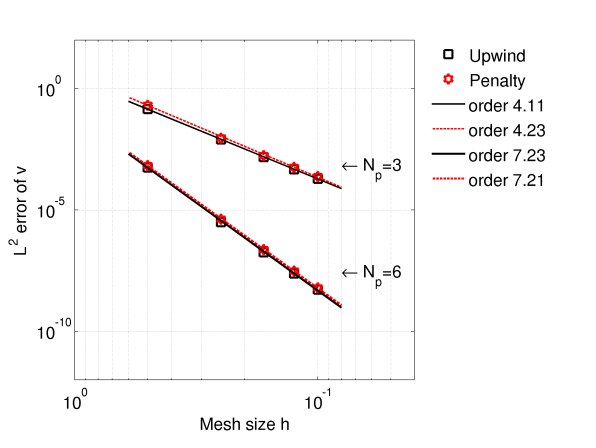
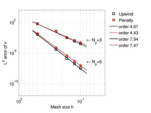
(A)	(B)
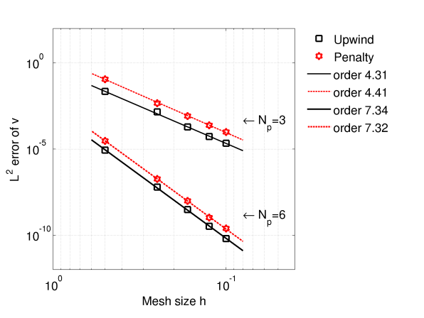
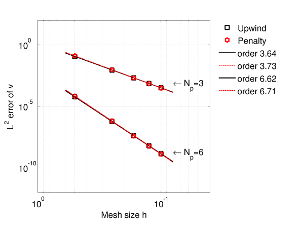
(C)	(D)

Figure 12: comparison of the accuracies and convergence rates between the penalized numerical fluxes and the upwind flux when simulating (A) a plane wave, (B) a Rayleigh wave, (C) a Stoneley wave, and (D) a Scholte wave, for different orders $N_{p}=3$ and $6$.

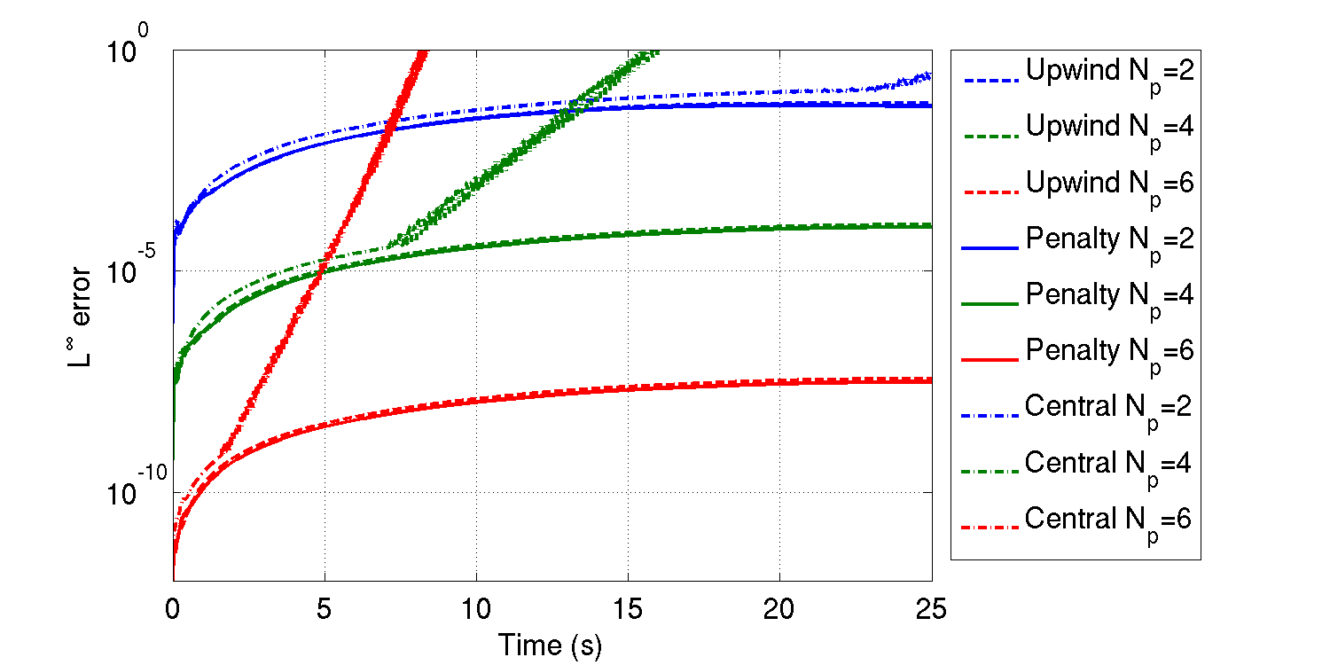
Figure 13: Accuracy as a function for propagation time of three types of numerical fluxes for the simulation of a Scholte wave. The maximum propagation time is $25$ s, which corresponds with a distance of $5.4$ wavelengths; $h=0.25$km ($0.125$ wavelengths). When the numerical method starts to blow up, the error function increases exponentially and the curve becomes jittery.

Figure 12 compares the accuracies and convergence rates of the penalized numerical fluxes with the upwind flux when simulating a plane wave (A), a Rayleigh wave (B), a Stoneley wave (C) and a Scholte wave (D), for both the lower-order case ($N_{p}=3$) and the relatively higher-order case ($N_{p}=6$). We observe that the measured errors for the penalized flux are sometimes slightly larger than those for the upwind flux, while the orders of convergence are essentially the same (and both better than $\mathcal{O}(h^{N_{p}+\frac{1}{2}})$).

Figure 13 shows the time dependent error measure for all three types of numerical fluxes. We simulate the Scholte wave for 25 seconds, with uniform mesh size $h=0.125$km and order $N_{p}=2,4,6$ for each numerical flux. The central flux turns out to be unstable with growing oscillatory numerical errors during time evolution. This instability may be caused by the inaccuracy of numerical integration, in which case the integration by parts does not necessary hold, and the energy-conserving property no longer holds. In comparison, the upwind and penalty fluxes extend the tolerance to inexact numerical integration.

References

- [Achenbach(1973)] Achenbach, J. D., 1973. Wave propagation in elastic solids, vol. 16, North-Holland Amsterdam.
- [Appelö & Petersson(2009)] Appelö, D. & Petersson, N. A., 2009. A stable finite difference method for the elastic wave equation on complex geometries with free surfaces, Communications in Computational Physics, 5(1), 84–107.
- [Ascher et al.(1997)Ascher, Ruuth, & Spiteri] Ascher, U. M., Ruuth, S. J., & Spiteri, R. J., 1997. Implicit-explicit Runge-Kutta methods for time-dependent partial differential equations, Applied Numerical Mathematics, 25(2), 151–167.
- [Bermúdez et al.(1999)Bermúdez, Hervella-Nieto, & Rodrıguez] Bermúdez, A., Hervella-Nieto, L., & Rodrıguez, R., 1999. Finite element computation of three-dimensional elastoacoustic vibrations, Journal of Sound and Vibration, 219(2), 279–306.
- [Blazek et al.(2013)Blazek, Stolk, & Symes] Blazek, K. D., Stolk, C., & Symes, W. W., 2013. A mathematical framework for inverse wave problems in heterogeneous media, Inverse Problems, 29(6), 065001.
- [Carcione(1994)] Carcione, J. M., 1994. The wave equation in generalized coordinates, Geophysics, 59(12), 1911–1919.
- [Carrington et al.(2008)Carrington, Komatitsch, Laurenzano, Tikir, Michéa, Le Goff, Snavely, & Tromp] Carrington, L., Komatitsch, D., Laurenzano, M., Tikir, M. M., Michéa, D., Le Goff, N., Snavely, A., & Tromp, J., 2008. High-frequency simulations of Global seismic wave propagation using SPECFEM3D_GLOBE on 62K processors, pp. 60:1–60:11.
- [Chaljub & Valette(2004)] Chaljub, E. & Valette, B., 2004. Spectral element modelling of three-dimensional wave propagation in a self-gravitating Earth with an arbitrarily stratified outer core, Geophysical Journal International, 158(1), 131–141.
- [Chaljub et al.(2003)Chaljub, Capdeville, & Vilotte] Chaljub, E., Capdeville, Y., & Vilotte, J.-P., 2003. Solving elastodynamics in a fluid–solid heterogeneous sphere: a parallel spectral element approximation on non-conforming grids, Journal of Computational Physics, 187(2), 457–491.
- [Chung & Engquist(2006)] Chung, E. T. & Engquist, B., 2006. Optimal discontinuous Galerkin methods for wave propagation, SIAM Journal on Numerical Analysis, 44(5), 2131–2158.
- [Cockburn & Shu(2001)] Cockburn, B. & Shu, C.-W., 2001. Runge–Kutta discontinuous Galerkin methods for convection-dominated problems, Journal of scientific computing, 16(3), 173–261.
- [De Basabe et al.(2008)De Basabe, Sen, & Wheeler] De Basabe, J. D., Sen, M. K., & Wheeler, M. F., 2008. The interior penalty discontinuous Galerkin method for elastic wave propagation: grid dispersion, Geophysical Journal International, 175(1), 83–93.
- [Dumbser & Käser(2006)] Dumbser, M. & Käser, M., 2006. An arbitrary high-order discontinuous Galerkin method for elastic waves on unstructured meshes–II. the three-dimensional isotropic case, Geophysical Journal International, 167(1), 319–336.
- [Etienne et al.(2010)Etienne, Chaljub, Virieux, & Glinsky] Etienne, V., Chaljub, E., Virieux, J., & Glinsky, N., 2010. An hp-adaptive discontinuous Galerkin finite-element method for 3-D elastic wave modelling, Geophysical Journal International, 183(2), 941–962.
- [Fehler & Keliher(2011)] Fehler, M. & Keliher, P. J., 2011. SEAM Phase 1: Challenges of Subsalt Imaging in Tertiary Basins, with Emphasis on Deepwater Gulf of Mexico, Society of Exploration Geophysicists Tulsa.
- [Graves(1996)] Graves, R. W., 1996. Simulating seismic wave propagation in 3d elastic media using staggered-grid finite differences, Bulletin of the Seismological Society of America, 86(4), 1091–1106.
- [Grote et al.(2006)Grote, Schneebeli, & Schötzau] Grote, M. J., Schneebeli, A., & Schötzau, D., 2006. Discontinuous Galerkin finite element method for the wave equation, SIAM Journal on Numerical Analysis, 44(6), 2408–2431.
- [Henderson(2007)] Henderson, A., 2007. ParaView Guide, A Parallel Visualization Application, Kitware Inc.
- [Hesthaven & Warburton(2007)] Hesthaven, J. S. & Warburton, T., 2007. Nodal discontinuous Galerkin methods: algorithms, analysis, and applications, vol. 54, Springer.
- [Igel(1999)] Igel, H., 1999. Wave propagation in three-dimensional spherical sections by the Chebyshev spectral method, Geophysical Journal International, 136(3), 559–566.
- [Kanevsky et al.(2007)Kanevsky, Carpenter, Gottlieb, & Hesthaven] Kanevsky, A., Carpenter, M. H., Gottlieb, D., & Hesthaven, J. S., 2007. Application of implicit-explicit high order Runge–Kutta methods to discontinuous-Galerkin schemes, Journal of Computational Physics, 225(2), 1753 – 1781.
- [Käser & Dumbser(2008)] Käser, M. & Dumbser, M., 2008. A highly accurate discontinuous Galerkin method for complex interfaces between solids and moving fluids, Geophysics, 73(3), T23–T35.
- [Kaufman & Levshin(2005)] Kaufman, A. A. & Levshin, A. L., 2005. Acoustic and elastic wave fields in geophysics, vol. 3, Elsevier.
- [Komatitsch & Martin(2007)] Komatitsch, D. & Martin, R., 2007. An unsplit convolutional perfectly matched layer improved at grazing incidence for the seismic wave equation, Geophysics, 72(5), SM155–SM167.
- [Komatitsch & Tromp(2002)] Komatitsch, D. & Tromp, J., 2002. Spectral-element simulations of global seismic wave propagation – I. validation, Geophysical Journal International, 149(2), 390–412.
- [Komatitsch & Vilotte(1998)] Komatitsch, D. & Vilotte, J.-P., 1998. The spectral element method: An efficient tool to simulate the seismic response of 2D and 3D geological structures, Bulletin of the seismological society of America, 88(2), 368–392.
- [Komatitsch et al.(2000)Komatitsch, Barnes, & Tromp] Komatitsch, D., Barnes, C., & Tromp, J., 2000. Wave propagation near a fluid-solid interface: A spectral-element approach, Geophysics, 65(2), 623–631.
- [Komatitsch et al.(2005)Komatitsch, Tsuboi, & Tromp] Komatitsch, D., Tsuboi, S., & Tromp, J., 2005. The spectral-element method in seismology, Geophysical Monograph Series, 157, 205–227.
- [Kozdon et al.(2013)Kozdon, Dunham, & Nordstr枚m] Kozdon, J., Dunham, E., & Nordstr枚m, J., 2013. Simulation of dynamic earthquake ruptures in complex geometries using high-order finite difference methods, Journal of Scientific Computing, 55(1), 92–124.
- [Li et al.(2009)Li, Petrovitch, & Pyrak-Nolte] Li, W., Petrovitch, C. L., & Pyrak-Nolte, L. J., 2009. The effect of fabric-controlled layering on compressional and shear wave propagation in carbonate rock, International Journal of the JCRM, 4(2), 79–85.
- [Lombard & Piraux(2004)] Lombard, B. & Piraux, J., 2004. Numerical treatment of two-dimensional interfaces for acoustic and elastic waves, Journal of Computational Physics, 195(1), 90–116.
- [Lombard et al.(2008)Lombard, Piraux, Gélis, & Virieux] Lombard, B., Piraux, J., Gélis, C., & Virieux, J., 2008. Free and smooth boundaries in 2-D finite-difference schemes for transient elastic waves, Geophysical Journal International, 172(1), 252–261.
- [Madariaga(1976)] Madariaga, R., 1976. Dynamics of an expanding circular fault, Bulletin of the Seismological Society of America, 66(3), 639–666.
- [Nurmi et al.(1990)Nurmi, Charara, Waterhouse, & Park] Nurmi, R., Charara, M., Waterhouse, M., & Park, R., 1990. Heterogeneities in carbonate reservoirs: detection and analysis using borehole electrical imagery, Geological Society, London, Special Publications, 48(1), 95–111.
- [Ohminato & Chouet(1997)] Ohminato, T. & Chouet, B. A., 1997. A free-surface boundary condition for including 3D topography in the finite-difference method, Bulletin of the Seismological Society of America, 87(2), 494–515.
- [Oristaglio(2012)] Oristaglio, M., 2012. SEAM Phase II–land seismic challenges, The Leading Edge, 31(3), 264–266.
- [Persson(2011)] Persson, P.-O., 2011. High-order LES simulations using implicit-explicit Runge–Kutta schemes, in Proceedings of the 49th AIAA Aerospace Sciences Meeting and Exhibit, AIAA, vol. 684.
- [Rivière & Wheeler(2000)] Rivière, B. & Wheeler, M. F., 2000. A discontinuous Galerkin method applied to nonlinear parabolic equations, in Discontinuous Galerkin Methods, pp. 231–244, Springer.
- [Robertsson(1996)] Robertsson, J. O., 1996. A numerical free-surface condition for elastic/viscoelastic finite-difference modeling in the presence of topography, Geophysics, 61(6), 1921–1934.
- [Si(2015)] Si, H., 2015. TetGen, a Delaunay-based quality tetrahedral mesh generator, ACM Trans. Math. Softw., 41(2), 11:1–11:36.
- [Smith et al.(2010)Smith, Collis, Ober, Overfelt, & Schwaiger] Smith, T. M., Collis, S. S., Ober, C. C., Overfelt, J. R., & Schwaiger, H. F., 2010. Elastic wave propagation in variable media using a discontinuous Galerkin method, SEG Epanded Abstracts, 29, 2982–2987.
- [Symes & Vdovina(2009)] Symes, W. & Vdovina, T., 2009. Interface error analysis for numerical wave propagation, Computational Geosciences, 13(3), 363–371.
- [Tessmer et al.(1992)Tessmer, Kessler, Kosloff, & Behle] Tessmer, E., Kessler, D., Kosloff, D., & Behle, A., 1992. Multi-domain Chebyshev-Fourier method for the solution of the equations of motion of dynamic elasticity, Journal of Computational Physics, 100(2), 355–363.
- [Virieux(1986)] Virieux, J., 1986. P-SV wave propagation in heterogeneous media: Velocity-stress finite-difference method, Geophysics, 51(4), 889–901.
- [Warburton(2006)] Warburton, T., 2006. An explicit construction of interpolation nodes on the simplex, Journal of Engineering Mathematics, 56(3), 247–262.
- [Warburton(2013)] Warburton, T., 2013. A low-storage curvilinear Discontinuous Galerkin method for wave problems, SIAM Journal on Scientific Computing, 35(4), A1987–A2012.
- [Wilcox et al.(2010)Wilcox, Stadler, Burstedde, & Ghattas] Wilcox, L. C., Stadler, G., Burstedde, C., & Ghattas, O., 2010. A high-order discontinuous Galerkin method for wave propagation through coupled elastic–acoustic media, Journal of Computational Physics, 229, 9373–9396.
- [Zienkiewicz & Bettess(1978)] Zienkiewicz, O. & Bettess, P., 1978. Fluid-structure dynamic interaction and wave forces. an introduction to numerical treatment, International Journal for Numerical Methods in Engineering, 13(1), 1–16.
- [Zingg(2000)] Zingg, D. W., 2000. Comparison of high-accuracy finite-difference methods for linear wave propagation, SIAM Journal on Scientific Computing, 22(2), 476–502.
- [Zingg et al.(1996)Zingg, Lomax, & Jurgens] Zingg, D. W., Lomax, H., & Jurgens, H., 1996. High-accuracy finite-difference schemes for linear wave propagation, SIAM Journal on Scientific Computing, 17(2), 328–346.