The Possible Orbital Decay and Transit Timing Variations of the Planet WASP-43b

Abstract

Motivated by the previously reported high orbital decay rate of the planet WASP-43b, eight newly transit light curves are obtained and presented. Together with other data in literature, we perform a self-consistent timing analysis with data covering a timescale of 1849 epochs. The results give an orbital decay rate $dP/dt$ = $-0.02890795\pm 0.00772547$ sec/year, which is one order smaller than previous values. This slow decay rate corresponds to a normally assumed theoretical value of stellar tidal dissipation factor. In addition, through the frequency analysis, the transit timing variations presented here are unlikely to be periodic, but could be signals of a slow orbital decay.

1 Introduction

The discoveries of new extra-solar planets continue to be exciting and have revealed many new implications about the formation and evolution of planetary systems. Though the majority of them was detected by the method of Doppler shift (Marcy & Butler 1998), other methods such as transit, direct imaging etc. also made impressed contributions. Because the orbital configurations of extra-solar planetary systems are generally quite different from our Solar system, many investigations on their dynamical properties and evolution have been done (see Jiang & Ip 2001, Ji et al. 2002, Jiang et al. 2003, Jiang & Yeh 2004a, Jiang & Yeh 2004b, Jiang & Yeh 2007, Mordasini et al. 2009). In addition, the further observational effort also produces new fruitful results continuously. For example, Kepler space telescope has discovered many multiple planetary systems through the transit method (Lissauer et al. 2011). Maciejewski et al. (2010) and Jiang et al. (2013) discovered possible transit timing variations (TTVs) which could imply the existence of additional bodies in these planetary systems. Lee et al. (2014) also found planetary companions around evolved stars through the method of radial velocities by Doppler shift.

Among these, those extreme systems with very short orbital period have particularly raised many interesting questions such as where they could have formed, how they would have migrated to current positions, and how stable their current orbits are etc. Their physical properties have also been seriously investigated with great effort. For example, WASP-12 planetary system, discovered by Hebb et al. (2009), was one of the well known extreme systems that attracted much attention. The planet was argued to be losing mass by exceeding its Roche lobe. Due to the falling of planetary gas towards the host star through the first Lagrange point, it is likely to form an accretion disk (Li et al. 2010). This might lead to the transfer of metals and thus enhance the stellar metallicity. Maciejewski et al. (2011) employed a high-precision photometric monitoring to study this system and greatly improved the determination of WASP-12b planetary properties.

On the other hand, the WASP-43 planetary system, first discovered by Hellier et al. (2011), is another case with an even smaller orbit. The planet is moving around a low mass K star with an orbital period only about 0.8 days. With a mass of 1.8 Jupiter Mass, it is one of the most massive exoplanets carrying an extremely short orbital period.

The existence of WASP-43 system has therefore triggered the study of thermal radiation from exoplanets. For example, Wang et al. (2013) confirmed the thermal emission from the planet WASP-43b. Chen et al.(2014) observed one transit and one occultation event in many bands simultaneously. They detected the day-side thermal emission in the $K$-band. Moreover, Kreidberg et al. (2014) determined the water abundance in the atmosphere of WASP-43b based on the observations through Hubble Space Telescope.

As discussed in Jiang et al. (2003), a system with a close-in planet would experience an orbital decay through star-planet tidal interactions. Indeed, through the XMM-Newton observations, Czesla et al. (2013) showed an X-ray detection and claimed that WASP-43 is an active K-star, which could be related with tidal interactions. In order to obtain more precise measurements of the characteristics of this system, Gillon et al. (2012) performed an intense photometric monitoring by ground-based telescopes. The physical parameters have been measured with much higher precision. Employing their data, the atmosphere of WASP-43b was modeled. However, they concluded that their transit data presented no sign of transit timing variations.

Later, through a timing analysis on the transits of WASP-43b, Blecic et al. (2014) proposed an orbital period decreasing rate about 0.095 second per year. With the data from Gran Telescopio Canarias (GTC), Murgas et al. (2014) also claimed an orbital decay with period decreasing rate about 0.15 second per year and suggested that a further timing analysis over future years would be important.

Motivated by the above interesting results, we employ two telescopes to monitor the WASP-43b transit events and obtain eight new transit light curves. Combining our own data with available published photometric transit data of WASP-43b, we investigate the possible timing variations or orbital decay here. Since these data cover more than 1800 epochs of the orbital evolution, our results shall serve as the most updated reference for this system. Our observational data are described in Section 2, the analysis of light curves is in Section 3, the results of transit timing variations are presented in Section 4, and finally the concluding remarks are provided in Section 5.

2 Observational Data

2.1 Observations and Data Reduction

In this project, two telescopes were employed to observe the transits of WASP-43b. One is the 1.25-meter telescope (AZT-11) at the Crimean Astrophysical Observatory (CrAO) in Nauchny, Crimea, and another is the 60-inch telescope (P60) at Palomar Observatory in California, USA. We successfully performed one complete transit observation with AZT-11 in 2012 and seven with P60 in 2014 and 2015. A summary of the above observations is presented in Table 1.

After some standard procedures such as flat-field corrections etc., we first use the IRAF task, $daofind$, to pick bright stars and then the task, $phot$, to measure these stars’ fluxes in each image. The light curves of these bright stars are thus determined (Jiang et al. 2013, Sun et al. 2015). In order to decide which stars could be comparison stars, we first choose those with higher brightness consistency as candidates, i.e. candidate stars. Therefore, we calculate the Pearson’s correlation coefficient between any two of these light curves and use 0.9 as the criterion. The candidate stars are a set of stars in which the correlation coefficient between any pairs of their light curves must be more than 0.9, in order to ensure the brightness consistency and that none of the candidate stars are variable objects. Finally, the flux of WASP-43 is divided by any possible combination of the fluxes from candidate stars. For example, when there are three candidate stars, the flux of WASP-43 is divided by the summation of all three candidate stars, the summation of any possible pairs from these candidate stars, and also the flux of individual candidate stars. Each of the above operations leads to one calibrated light curve, and the one with the smallest out-of-transit root-mean-square deviation becomes the light curve of WASP-43. Note that the out-of-transit root-mean-square deviation is determined after the normalization process, which would be described in Section 2.3 later. The comparison stars are those involved in the determination of the light curve of WASP-43. The number of bright stars, candidate stars, and comparison stars are listed in Table 2.

2.2 Other Observational Data from Literature

In addition to our own light curves, it will be very helpful to employ those publicly available transit data in previous work. With both our own and other transit light curves, we could therefore cover a large number of epochs for the investigation on possible transit timing variations. We review all WASP-43b papers and find that there are five papers in which the electronic files of transit light curves are provided.

Gillon et al. (2012) employed the 60cm telescope, TRAPPIST (TRAnsiting Planets and PlanetesImals Small Telescope), in the Astrodon $I+z$ filter to obtain 20 light curves and the 1.2m Euler Swiss telescope in the Gunn-$r^{\prime}$ filter to obtain three light curves. Two of the above light curves are actually for the same transit event. That is, Epoch 38 is observed by both telescopes. Note that the epochs are given an identification number following the convention that the transit observed in Hellier et al. (2011) is Epoch 0. Chen et al. (2014) observed the transit event of Epoch 499 with the GROND instrument mounted on 2.2m MPG/ESO telescope in seven bands: Sloan $g^{\prime},r^{\prime},i^{\prime},z^{\prime}$ and NIR $J,H,K$. We take the light curve in $J$ band, because only $J,H$, and $K$ bands have the information of seeing and the wavelength of $J$ band is the closest to $R$ band, the one we used for our own observations. Maciejewski et al. (2013) provided the light curves of Epoch 543 and Epoch 1032. Murgas et al. (2014) used GTC (Gran Telescopio Canarias) instrument OSIRIS to obtain long-slit spectra. We choose the white light-curve data to do the analysis in this paper. In addition, there are seven light curves available from Ricci et al.(2015).

Therefore, we take 23 light curves from Gillon et al. (2012). In addition, we get one light curve from Chen et al. (2014), two light curves from Maciejewski et al. (2013), one from Murgas et al. (2014), and seven from Ricci et al.(2015). In total, we have 34 light curves taken from published papers.

We do not simply use the mid-transit times written in these papers, but re-analyze all the photometric data with the same procedure and software to perform parameter fitting in a consistent way. Because all these data go through the same transit modeling and fitting procedure as our own data, it can ensure that the results are reliable.

2.3 The Normalization and Time Stamp of Light Curves

For all the previously mentioned light curves, including eight from our work and 34 from the published papers, we further consider the airmass and seeing effects here. As the procedure in Murgas et al. (2014), a 3rd-degree polynomial is used to model the airmass effect, and a linear function is employed to model the seeing effect. The original light curve, $F_{o}(t)$, can be expressed as:

$$F_{o}(t)=F(t)\mathcal{P}(t)\mathcal{Q}(s),$$ (1)

where $F(t)$ is the corrected light curve, $\mathcal{P}(t)=a_{0}+a_{1}t+a_{2}t^{2}+a_{3}t^{3}$, and $\mathcal{Q}(s)=1+c_{0}s$, where $s$ is the seeing of each image. (Note that, in Maciejewski et al. 2013 and Ricci et al. 2015, the seeing is not known and no seeing correction can be done. We thus set $\mathcal{Q}(s)=1$ for light curves from these two papers.) We numerically search the best values of five parameter $a_{0},a_{1},a_{2},a_{3},c_{0}$ to make out-of-transit part of $F(t)$ close to unity with smallest standard deviations, and thus normalize all the light curves. $F(t)$ would be simply called the observational light curves and used in any further analysis for the rest of this paper.

On the other hand, the time stamp we use is the Barycentric Julian Date in the Barycentric Dynamical Time ($BJD_{TDB}$). We compute the UT time of mid exposure from the recorded header and convert the time stamp to $BJD_{TDB}$ as in Eastman et al. (2010).

3 The Analysis of Light Curves

The Transit Analysis Package (TAP) presented by Gazak et al. (2012) is used to obtain transit models and corresponding parameters from all the above 42 light curves. TAP employs the light-curve models of Mandel & Agol (2002), the wavelet-based likelihood function developed by Carter & Winn (2009), and Markov Chain Monte Carlo (MCMC) technique to determine the parameters.

All 42 light curves are loaded into TAP and analyzed simultaneously. For each light curve, five MCMC chains of length 500,000 are computed. To start an MCMC chain in TAP, we need to set the initial values of the following parameters: orbital period $P$, orbital inclination $i$, semi-major axis $a$ (in the unit of stellar radius $R_{\ast}$), the planet’s radius $R_{\rm p}$ (in the unit of stellar radius), the mid-transit time $T_{\rm m}$, the linear limb darkening coefficient $u_{1}$, the quadratic limb darkening coefficient $u_{2}$, orbital eccentricity $e$ and the longitude of periastron $\omega$. Once the initial values are set, one could choose any one of the above to be: (1) completely fixed (2) completely free to vary or (3) varying following a Gaussian function, i.e., Gaussian prior, during the MCMC chain in TAP. Moreover, any of the above parameters which is not completely fixed can be linked among different light curves. The orbital period is treated as a fixed parameter $P$ = 0.81347753, which is taken from Table 5 of Gillon et al. (2012). The initial values of inclination $i$, semi-major axis, and planet’s radius are all from Gillon et al.(2012), i.e. $i$=82.33, $a/R_{\ast}$=4.918, and $R_{\rm p}/R_{\ast}$=0.15945. They are completely free to vary and linked among all light curves. We leave the mid-transit times $T_{\rm m}$ to be completely free during TAP runs and it is only linked among those light curves in the same transit events. Two light curves from Gillon et al. (2012) are for the same transit event, i.e. epoch 38, and another two from Ricci et al. (2015) are for epoch 1469.

A Gaussian prior centered on the values of quadratic limb darkening coefficients with certain $\sigma$ are set for TAP runs. The quadratic limb darkening coefficients and $\sigma$ for $I+z$ and Gunn-$r^{\prime}$ filters are set as the values in Gillon et al. (2012), and the one for white light curve follows the values used in Murgas et al. (2014).

For $i,I,J,R$, and $V$ filters, we linearly interpolate from Claret (2000, 2004) to the values effective temperature $T_{\rm eff}$ = 4400 K, log$g$ = 4.5 ${\rm cm/s^{2}}$, metallicity [Fe/H] = 0, and micro-turbulent velocity $V_{\rm t}$ = 0.5 ${\rm km/s}$ (Hellier et al. 2011). In order to consider the possible small differences mentioned in Southworth (2008), a Gaussian prior centered on the theoretical values with $\sigma$ = 0.05 is set for our limb darkening coefficients $u_{1}$ and $u_{2}$ during TAP runs. The details of parameter setting for TAP runs are listed in Table 3 and Table 4.

There are five chains in each of our TAP runs, and all of the chains are added together into the final results. The 15.9, 50.0 and 84.1 percentile levels are recorded. The 50.0 percentile, i.e., median level, is used as the best value, and the other two percentile levels give the error bar.

The mid-transit time for the corresponding epoch of each transit event is obtained. In order to examine whether there is any outlier, these mid-transit times are fitted by a linear function. It is found that the mid-transit time of epoch 1469 has the largest deviation and is more than 3$\sigma$ away from the linear function. We thus remove two light curves of epoch 1469 from our data set and re-run TAP through the same procedure. We finally obtain the mid-transit time for the corresponding epoch of each transit event, as those presented in Table 5. They will be used to establish a new ephemeris and study the transit timing variations in next section. The results of inclination, semi-major axis, and planet’s radius are listed in Table 6. These values are consistent with all those published in previous work. For example, comparing with the results in Gillon et al.(2012) or Ricci et al (2015), our results are all extremely close to theirs, if error bars are considered. Our error bars are actually smaller than theirs. This shows that our analysis with more light curves gives stronger observational constraints.

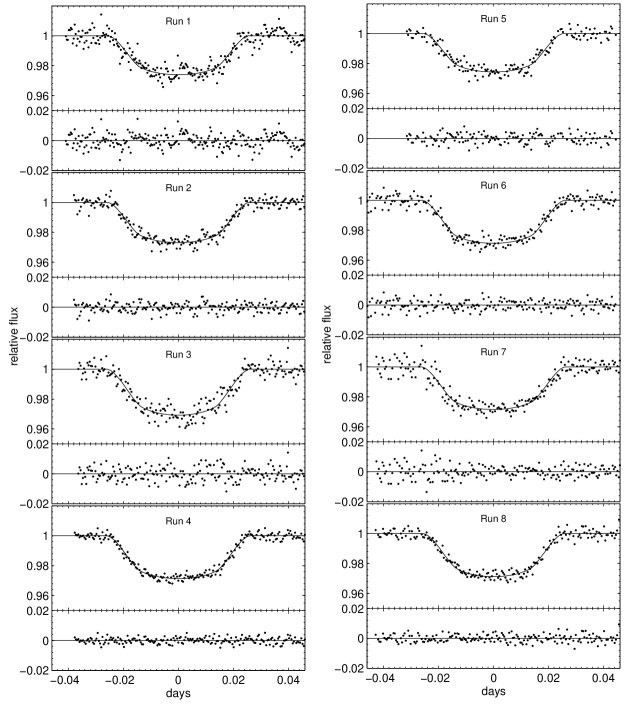
Figure 1: The normalized relative flux as a function of the time (the offset from mid-transit time and in TDB-based BJD) of eight transit light curves of this work: points are the data and curves are models. The corresponding residuals are shown at the bottom of light curves.

Moreover, the observational light curves and best fitting models of our own data are presented in Figure 1, where the points are observational data and solid curves are the best fitting models. These eight light curves of our own work are available in a machine-readable form in the electronic version of Table 7.

4 Transit Timing Variations

4.1 A New Ephemeris

When all mid-transit times of 39 epochs in Table 5 are considered, we obtain a new ephemeris by minimizing $\chi^{2}$ through fitting a linear function as

$$T^{C}_{\rm m}(E)=T_{0}+PE,$$ (2)

where $T_{0}$ is a reference time, $E$ is an epoch (The transit observed in Hellier et al. 2011 is defined to be epoch $E=0$, and other transits’ epochs are defined accordingly.), $P$ is the orbital period, and $T^{C}_{\rm m}(E)$ is the calculated mid-transit time at a given epoch $E$.

We find that $T_{0}=2455528.86860518\pm 0.00003632$ ($BJD_{TDB}$), $P=0.81347392\pm 0.00000004$ (day). The corresponding $\chi^{2}$ = 266.2076. Because the degree of freedom is 37, the reduced $\chi^{2}$, $\chi^{2}_{red}(37)$ = 7.1948. Using this new ephemeris, the $O-C$ diagram is presented as the data points in Figure 2. The large value of reduced $\chi^{2}$ of the linear fitting presented here indicates that a certain level of TTVs does exist.

4.2 A Model of Orbital Decay

Through the transit timing analysis, Blecic et al. (2014) and Murgas et al. (2014) proposed a possible orbital decay for the planet WASP-43b. However, their transit data were up to about epoch 1000 only. It would be very interesting to see whether our newly observed data gives the transit timing with a trend of orbital decay.

Assume the orbital period is $P_{q}$, and the predicted mid-transit time at epoch $E$ is $T_{S}(E)$. For convenience, the mid-transit time of epoch 0, $T_{S}(0)$, is set to be zero, so the mid-transit time of epoch 1 is $T_{S}(1)=P_{q}$, and the elapsed time $\delta t_{1}=P_{q}$. If there is a small amount of period changing $\delta P$ from time $t=T_{S}(1)$ to $t=T_{S}(2)$, the elapsed time is $\delta t_{2}=P_{q}+\delta P$. Suppose there is a further period changing with $\delta P$ from time $t=T_{S}(2)$ to $t=T_{S}(3)$, so the elapsed time $\delta t_{3}=P_{q}+2\delta P$. Following this continuous period decay, we have $\delta t_{i}=P_{q}+(i-1)\delta P$, where $i=1,2,...,(E-1),E$. Summing up all the above $\delta t_{i}$, we obtain $T_{S}(E)=EP_{q}+[E(E-1)/2]\delta P$.

Therefore, as in Blecic et al. (2014), a model of orbital decay can be obtained by minimizing $\chi^{2}$ through fitting a function as

$$T_{S}(E)=T_{q0}+P_{q}E+\delta P\frac{E(E-1)}{2}$$ (3)

where $T_{q0}$ is a reference time, $E$ is an epoch, $P_{q}$ is the orbital period, $\delta P$ is the amount of period changing between each mid-transit time starting from $t=T_{S}(1)$.

When only the data of earlier work with transits before epoch 1100, i.e. Gillon et al. (2012), Chen et al. (2014), Maciejewski et al. (2013), and Murgas et al. (2014), are considered, we have $T_{q0}=2455528.86809115\pm 0.00006471$, $P_{q}=0.81347925\pm 0.00000055$, $\delta P=-1.03181346\times 10^{-8}\pm 0.10711789\times 10^{-8}$. The corresponding $\chi^{2}$= 131.7672, and $\chi^{2}_{red}(24)=5.4903$. Using the above best-fitted parameters for $T_{S}(E)$ and the new ephemeris for $T^{C}_{\rm m}(E)$, the $T_{S}(E)-T^{C}_{\rm m}(E)$ as a function of epoch $E$ is plotted as the dashed curve in the $O-C$ diagram, together with data points as shown in Figure 2. Both the units of $P_{q}$ and $\delta P$ are days, and we obtain $dP/dt=\delta P/P_{q}$ = $-0.40027520\pm 0.04155436$ sec/year. We find that this result is consistent with the orbital decay rate stated in previous works.

When all the data in Table 5 are considered, we obtain $T_{q0}=2455528.86851783\pm 0.00004318$, $P_{q}=0.81347448\pm 0.00000016$, $\delta P=-7.45173434\times 10^{-10}\pm 1.98109164\times 10^{-10}$. The corresponding $\chi^{2}_{red}(36)=7.0057$. The larger value of reduced $\chi^{2}$ is due to the larger number of data points in this case. Using the above best-fitted parameters for $T_{S}(E)$ and the new ephemeris for $T^{C}_{\rm m}(E)$, the $T_{S}(E)-T^{C}_{\rm m}(E)$ as a function of epoch $E$ is plotted as the solid curve in the $O-C$ diagram, together with data points as shown in Figure 2. Comparing the solid curve with the dashed curve in Figure 2, it is obvious that the data points around epoch 1500 and epoch 1900 do not follow the dashed curve. That is, the newly obtained transits do not follow the predicted transit timings in previous models.

On the other hand, for the solid curve in Figure 2, the overall orbital decay rate is $dP/dt=\delta P/P_{q}$ = $-0.02890795\pm 0.00772547$ sec/year, which is one order smaller than the values in previous work. Therefore, with our newly observed transits, we obtain a very different orbital decay rate. These results indicate that, if there is any orbital decay, the decay rate shall be much smaller than those values proposed in previous works. This slower orbital decay rate leads to a new estimate of the stellar tidal dissipation factor $Q_{\ast}$. Following the equation in Blecic et al. (2014), we obtain a value of $Q_{\ast}$ about the order of $10^{5}$, which is within the range of normally assumed theoretical value from $10^{5}$ to $10^{10}$.

4.3 The Frequency Analysis

In order to search for possible periodicities of transit timing variations from the timing residuals, Lomb-Scargle normalized periodogram (Press & Rybicki 1989) is used. Figure 3 shows the resulting spectral power as a function of frequencies. The false-alarm probability of the largest power of frequencies is 0.20, which is very far from the usual thresholds 0.05 or 0.01 for a confirmed frequency. Therefore, our results show that there is no evidence for periodic TTVs.

5 Concluding Remarks

Employing telescopes at two observatories, we monitor the transits of exoplanet WASP-43b and obtain eight new transit light curves. Together with the light curves from published papers, they are all further analyzed through the same procedure. The transit timings are obtained, and a new ephemeris is established. The newly determined inclination $i=82.149^{+0.084}_{-0.086}$, semi-major axis $a/R_{\ast}=4.837^{+0.021}_{-0.022}$, and planet’s radius $R_{\rm p}/R_{\ast}=0.15929^{+0.00045}_{-0.00045}$ are all consistent with previous work.

Our results reconfirm that a certain level of TTVs does exist, which is the same as what was claimed in Blecic et al.(2014) and Murgas et al.(2014) previously. However, the results here show that the transit timings of new data do not follow the fast trend of the orbital decay suggested in Blecic et al. (2014) and Murgas et al. (2014). Our results lead to an orbital decay rate $dP/dt$ = $-0.02890795\pm 0.00772547$ sec/year, which is one order smaller than the previous values. This slower rate corresponds to a larger stellar tidal dissipation factor $Q_{\ast}$ in the range of normally assumed theoretical value.

On the other hand, the false-alarm probabilities in the frequency analysis indicate that these TTVs are unlikely to be periodic. The TTVs we present here could be signals of a slow orbital decay.

We conclude that, in order to further investigate and understand this interesting system, both realistic theoretical modeling and much more high-precision observations are desired in the future.

Table 1: The log of observations of this work

Run	UT Date	Instrument	Filter	Interval (JD-2450000)	Exposure	No. of Images
1	2012 Mar 24	AZT-11	R	6011.212 - 6011.302	30	251
2	2014 Mar 12	P60	R	6728.698 - 6728.789	10	219
3	2014 Mar 16	P60	R	6732.767 - 6732.856	10	213
4	2014 Apr 07	P60	R	6754.731 - 6754.820	12	205
5	2014 Dec 24	P60	R	7015.864 - 7015.940	12	150
6	2015 Jan 06	P60	R	7028.864 - 7028.955	12	194
7	2015 Jan 15	P60	R	7037.815 - 7037.905	12	190
8	2015 Jan 19	P60	R	7041.882 - 7041.979	12	194

Table 1: The log of observations of this work. For each run, the UT date, instrument, filter, observational interval (JD-2450000), exposure time (second), and the number of images are listed.

Table 2: The numbers of stars

Run	No. of Brighter Stars	No. of Candidates	No. of Comparisons	oot rms
1	5	3	1	0.0045
2	18	3	3	0.0028
3	12	4	2	0.0041
4	24	5	2	0.0020
5	5	2	2	0.0029
6	11	2	2	0.0035
7	16	3	3	0.0042
8	13	10	6	0.0027

Table 2: The number of stars in the process for choosing comparison stars. The out-of-transit root-mean-square of light curves are also listed.

Table 3: The parameter setting

Parameter	Initial Value	During MCMC Chains
$P$(day)	0.81347753	fixed
$i$(deg)	82.33	free, linked among all
$a$/$R_{\ast}$	4.918	free, linked among all
$R_{\rm p}$/$R_{\ast}$	0.15945	free, linked among all
$T_{\rm m}$	set-by-eye	free, only linked if same transit events
$u_{1}$	Claret (2000,2004)	a Gaussian prior, not linked
$u_{2}$	Claret (2000,2004)	a Gaussian prior, not linked
$e$	0.0	fixed
${\omega}$	0.0	fixed

Table 3: The parameter setting. The initial values of $P,i,a/R_{\ast},R_{\rm p}/R_{\ast}$ are adopted from Table 5 of Gillon et al.(2012).

Table 4: The quadratic limb darkening coefficients

filter	$u_{1}$	$u_{2}$
${}^{a}I+z$	$0.440\pm 0.035$	$0.180\pm 0.025$
aGunn-$r^{\prime}$	$0.625\pm 0.015$	$0.115\pm 0.010$
bwhite	$0.394\pm 0.087$	$0.289\pm 0.119$
${}^{c}i$	$0.4767\pm 0.05$	$0.2067\pm 0.05$
${}^{c}I$	$0.4401\pm 0.05$	$0.2200\pm 0.05$
${}^{c}J$	$0.2560\pm 0.05$	$0.2959\pm 0.05$
${}^{c}R$	$0.6012\pm 0.05$	$0.1492\pm 0.05$
${}^{c}V$	$0.7598\pm 0.05$	$0.0427\pm 0.05$
dclear	$0.6805\pm 0.05$	$0.0960\pm 0.05$

Table 4: The quadratic limb darkening coefficients.
^aset as the values in Gillon et al. (2012)
^bset as the values in Murgas et al. (2014)
^ccalculated for $T_{\rm eff}=4400$ K, log$g$ = 4.5 ${\rm cm/s^{2}}$, [Fe/H] = 0, and $V_{\rm t}$ = 0.5 ${\rm km/s}$.
^dcalculated as the average of those for $V$ and $R$ bands.

Table 5: The results of light-curve analysis for the mid-transit time

Epoch	Data Source	$T_{m}$($BJD_{TDB}-2450000$)
11	(a)	5537.81659 ${}^{+0.00045}_{-0.00048}$
22	(a)	5546.76493 ${}^{+0.00020}_{-0.00021}$
27	(a)	5550.83218 ${}^{+0.00019}_{-0.00018}$
38	(a)	5559.78048 ${}^{+0.00012}_{-0.00012}$
43	(a)	5563.84773 ${}^{+0.00021}_{-0.00020}$
49	(a)	5568.72833 ${}^{+0.00012}_{-0.00012}$
59	(a)	5576.86368 ${}^{+0.00015}_{-0.00015}$
65	(a)	5581.74392 ${}^{+0.00011}_{-0.00011}$
70	(a)	5585.81297 ${}^{+0.00029}_{-0.00029}$
76	(a)	5590.69256 ${}^{+0.00019}_{-0.00018}$
87	(a)	5599.64047 ${}^{+0.00024}_{-0.00024}$
97	(a)	5607.77505 ${}^{+0.00012}_{-0.00012}$
124	(a)	5629.73981 ${}^{+0.00011}_{-0.00010}$
140	(a)	5642.75474 ${}^{+0.00013}_{-0.00013}$
141	(a)	5643.56875 ${}^{+0.00023}_{-0.00022}$
152	(a)	5652.51574 ${}^{+0.00038}_{-0.00038}$
168	(a)	5665.53206 ${}^{+0.00026}_{-0.00026}$
173	(a)	5669.59939 ${}^{+0.00017}_{-0.00018}$
189	(a)	5682.61543 ${}^{+0.00018}_{-0.00018}$
200	(a)	5691.56374 ${}^{+0.00013}_{-0.00013}$
211	(a)	5700.51237 ${}^{+0.00018}_{-0.00018}$
243	(a)	5726.54407 ${}^{+0.00018}_{-0.00018}$
499	(b)	5934.79276 ${}^{+0.00019}_{-0.00019}$
543	(c)	5970.58598 ${}^{+0.00025}_{-0.00027}$
593	(f)	6011.25910 ${}^{+0.00056}_{-0.00054}$
950	(d)	6301.66872 ${}^{+0.00006}_{-0.00005}$
1032	(c)	6368.37476 ${}^{+0.00060}_{-0.00068}$
1442	(e)	6701.89857 ${}^{+0.00016}_{-0.00017}$
1475	(f)	6728.74255 ${}^{+0.00023}_{-0.00024}$
1480	(f)	6732.80936 ${}^{+0.00049}_{-0.00047}$
1485	(e)	6736.87743 ${}^{+0.00046}_{-0.00048}$
1486	(e)	6737.69125 ${}^{+0.00022}_{-0.00022}$
1496	(e)	6745.82472 ${}^{+0.00034}_{-0.00035}$
1507	(f)	6754.77378 ${}^{+0.00016}_{-0.00016}$
1550	(e)	6789.75311 ${}^{+0.00033}_{-0.00033}$
1828	(f)	7015.89837 ${}^{+0.00025}_{-0.00024}$
1844	(f)	7028.91466 ${}^{+0.00024}_{-0.00023}$
1855	(f)	7037.86178 ${}^{+0.00029}_{-0.00028}$
1860	(f)	7041.92985 ${}^{+0.00020}_{-0.00020}$

Table 5: The results of light-curve analysis for the mid-transit time $T_{m}$.
The epoch is the number of transit calculated from the first transit presented in Hellier et al. (2011). Data sources: (a) Gillon et al.(2012), (b) Chen et al.(2014), (c) Maciejewski et al.(2013), (d) Murgas et al.(2014), (e) Ricci et al.(2015), and (f) this work.

Table 6: The results of light-curve analysis for the inclination, semi-major axis, and planet’s radius

Parameter	Value
$i$	82.149 ${}^{+0.084}_{-0.086}$
$a$/$R_{\ast}$	4.837 ${}^{+0.021}_{-0.022}$
$R_{\rm p}$/$R_{\ast}$	0.15929 ${}^{+0.00045}_{-0.00045}$

Table 6: The results of light-curve analysis for the inclination $i$, semi-major axis $a$/$R_{\ast}$, and planet’s radius $R_{\rm p}$/$R_{\ast}$.

Table 7: The photometric light-curve data of this work

Run	Epoch	TDB-based BJD	Relative Flux
1	593	2456011.21824144	0.999658
		2456011.21859823	0.997367
		2456011.21895503	0.997222
2	1475	2456728.70459992	1.005345
		2456728.70501139	1.002147
		2456728.70542342	1.001576
3	1480	2456732.77312609	0.999979
		2456732.77353873	1.004087
		2456732.77395244	1.002193

Table 7: The photometric light-curve data of this work. This table is available in its entirety in the on-line journal. A portion is shown here for guidance.

Figure 2: The $O-C$ diagram. The filled circles are for our work. The triangles are for the data from Gillon et al. (2012), the square is for the data from Chen et al. (2014), the diamonds are for the data from Maciejewski et al. (2013), the cross is for the data from Murgas et al. (2014), and the open circles are for the data from Ricci et al. (2015). The dashed curve is the model determined by fitting with those data before epoch 1100 only. The solid curve is the model determined by fitting with all data.

Figure 3: The spectral power as a function of frequencies for the data points shown in Figure 2. The false-alarm probability of the largest power of frequencies is 0.20 and shown as the bottom dotted line. The middle dotted line shows 0.05, and the top dotted line shows 0.01 false-alarm probability.

References

- (1) Blecic, J. et al. 2014, ApJ, 781, 116
- (2) Carter, J. A. & Winn, J. N. 2009, ApJ, 704, 51
- (3) Chen, G. et al. 2014, A&A, 563, A40
- (4) Claret, A. 2000, A&A, 363, 1081
- (5) Claret, A. 2004, A&A, 428, 1001
- (6) Czesla, S., Salz, M., Schneider, P. C., Schmitt, J. H. M. M. 2013, A&A, 560, A17
- (7) Eastman, J., Siverd, R., & Gaudi, B. S. 2010, PASP, 122, 935
- (8) Gazak, J. Z. et al. 2012, Advances in Astronomy, 2012, 697967
- (9) Gillon, M. et al. 2012, A&A, 542, A4
- (10) Hebb, L. et al. 2009, ApJ, 693, 1920
- (11) Hellier, C. et al. 2011, A&A, 535, L7
- (12) Ji, J., Li, G., Liu, L. 2002, ApJ, 572, 1041
- (13) Jiang, I.-G., Ip, W.-H. 2001, A&A, 367, 943
- (14) Jiang, I.-G., Ip, W.-H., Yeh, L.-C. 2003, ApJ, 582, 449
- (15) Jiang, I.-G., Yeh, L.-C. 2004a, AJ, 128, 923
- (16) Jiang, I.-G., Yeh, L.-C. 2004b, Int. J. Bifurcation and Chaos, 14, 3153
- (17) Jiang, I.-G., Yeh, L.-C. 2007, ApJ, 656, 534
- (18) Jiang, I.-G. et al. 2013, AJ, 145, 68
- (19) Kreidberg, L. et al. 2014, ApJ, 793, L27
- (20) Lee, B.-C., Han, I., Park, M.-G., Mkrtichian, D. E., Hatzes, A. P., Kim, K.-M. 2014, A&A, 566, A67
- (21) Li, S.-L., Miller, N., Lin, D. N. C., Fortney, J. J. 2010, Nature, 463, 1054
- (22) Lissauer, J. J. et al. 2011, ApJS, 197, 8
- (23) Maciejewski, G. et al. 2010, MNRAS, 407, 2625
- (24) Maciejewski, G. et al. 2011, A&A, 528, A65
- (25) Maciejewski, G. et al. 2013, Information Bulletin on Variable Stars, 6082, 1
- (26) Marcy, G. W., Butler, R. P. 1998, ARA&A, 36, 57
- (27) Mandel, K. & Agol, E. 2002, ApJ, 580, L171
- (28) Mordasini, C., Alibert, Y., Benz, W. 2009, A&A, 501, 1139
- (29) Murgas, F. et al. 2014, A&A, 563, A41
- (30) Press, W. H. & Rybicki, G. B. 1989, ApJ, 388, 277
- (31) Ricci, D. et al. 2015, PASP, 127, 143
- (32) Sun, L.-L. et al. 2015, Research in Astronomy and Astrophysics, 15, 117
- (33) Southworth, J. 2008, MNRAS, 386, 1644
- (34) Wang, W., van Boekel, R., Madhusudhan, N., Chen, G., Zhao, G., Henning, Th. 2013, ApJ, 770, 70