Higgs boson production and decay in 5D warped models

Abstract

We calculate the production and decay rates of the Higgs boson at the LHC in the context of general 5 dimensional (5D) warped scenarios with a spacetime background modified from the usual $AdS_{5}$, with SM fields propagating in the bulk. We extend previous work by considering the full flavor structure of the SM, and thus including all possible flavor effects coming from mixings with heavy fermions. We proceed in three different ways, first by only including two complete Kaluza-Klein (KK) levels ($15\times 15$ fermion mass matrices), then including three complete KK levels ($21\times 21$ fermion mass matrices) and finally we compare with the effect of including the infinite (full) KK towers. We present numerical results for the Higgs production cross section via gluon fusion and Higgs decay branching fractions in both the modified metric scenario and in the usual Randall-Sundrum metric scenario.

I Introduction

The discovery of a light Higgs-like boson at the first run of the LHC seems to have provided an answer to the question of the origin of particle masses. While the particle discovered resembles very much the Standard Model (SM) Higgs boson, variations from the predicted coupling strengths of the SM are possible Aad:2015gba ; Chatrchyan:2012xdj .

These variations would be related to models beyond the SM, which address some of the shortcomings of the current theory such as the hierarchy problem or the flavor puzzle. Unfortunately the LHC has not yet provided an unequivocal signal for physics beyond the SM (supersymmetry, extra-dimensions) and such new physics scenarios could manifest themselves in some spectacular signal to be yet detected at Run II of the LHC. But they could also arise from a precise and careful measurement of the properties of the newly discovered boson, such as its mass, its couplings, its width or its production and decay rates.

In this work we investigate the signal strengths for gluon fusion production as well as tree-level and loop-dependent couplings for a broad class of models in which the space-time is extended to a warped geometry model with a five-dimensional background space-time metric. The initial incentive for these models was to solve the weak-Planck scale hierarchy by allowing gravity to propagate in the bulk of the extra dimension Randall:1999vf which has to be stabilized stabilization . Later it was realized that by allowing the SM fermion fields to propagate into the bulk, different geographical localization of fields along the extra dimension could help explain the observed masses and flavor mixing among quarks and leptons Davoudiasl:1999tf ; Pomarol:1999ad ; Grossman:1999ra ; Chang:1999nh ; Gherghetta:2000qt ; Davoudiasl:2000wi . Electroweak symmetry breaking can still happen via a standard Higgs mechanism in these scenarios (although the Higgs can also be implemented as as pseudo-Nambu-Goldstone boson) Contino:2003ve ; Csaki:2008zd . The Higgs boson itself must be located near the TeV boundary of the extra dimension in order to solve the hierarchy problem, and so typically it is assumed to be exactly localized on that boundary (brane Higgs scenario). Nevertheless, it is possible that it leaks out into the bulk (bulk Higgs scenario), and in doing so, indirectly it can alleviate some of the flavor bounds and precision electroweak tests plaguing these models Carena:2004zn ; Huber:2003tu ; Agashe:2004cp ; Agashe:2006at ; Csaki:2008qq . In order to satisfy the current bounds from precision flavor and electroweak processes, and still have light enough new physics to be seen at the LHC, one viable alternative is to extend the gauge group Agashe:2003zs ; Agashe:2006at . Another possibility is to modify the warping of the space-time metric, which can also alleviate some of the more stringent bounds Falkowski ; Batell ; Cabrer:2011fb ; Carmona:2011ib ; MertAybat:2009mk . In this work we focus on this last option.

In a previous work, we investigated Higgs boson production when allowed to propagate in the bulk both using the original Randall-Sundrum (RS) metric Frank:2013un , and also within a modified metric background Frank:2013qma . We analyzed the Higgs production rate via gluon fusion and showed that the results are consistent with the LHC Higgs measurements, in the same region of the parameter space where flavor and precision electroweak constraints are safe.

However, in both of these instances, our analyses employed a toy-model setup, in which the Higgs field was allowed to propagate in the bulk accompanied by a single 5D fermion field. Here, we extend our results to a realistic model with three families and include the full flavor effects. In addition to production cross section, we also analyze the Higgs couplings to quarks and leptons as well as the branching ratio for the di-photon decay. We include results from analyzing the model with a cut-off scale, and including two or three KK fermion levels only. We then compare these results with those obtained including the complete (infinite) tower of KK modes. We present the results for the model with the modified metric, $MAdS_{5}$, as well as the results within the original metric, whose effects on Higgs physics with full flavor was also studied in Archer:2014jca .

Our work is organized as follows. In Sec. II we introduce our model and discuss the limits imposed on its parameter space from precision measurements. In Sec. III we analyze the effects of the KK modes on gluon fusion production of the Higgs boson, assuming a finite number of KK modes (2 KK levels, then 3 KK levels). The same investigation for the $h\to\gamma\gamma$ coupling is presented in Sec. IV. Sec. V presents a detailed analysis of the procedure involved in calculating the inclusion of the infinite tower of KK fermions including three families of fermions. We then summarize our findings and conclude in Sec. VI.

II The $MAdS_{5}$ Model

Models with general warped extra space dimensions ($MAdS_{5}$) are characterized by the following metric Randall:1999vf

$$ds^{2}=e^{-2A(y)}\eta_{\mu\nu}dx^{\mu}dx^{\nu}+dy^{2},$$ (1)

where $\eta_{\mu\nu}=\text{diag}(-1,1,1,1)$ and $A(y)$ is a function of the extra space dimension originally (in RS models) assumed to be

$$A(y)=ky,$$ (2)

with $k$ being the inverse curvature radius of the $AdS_{5}$ space-time. In these models the extra dimension, $y$, is bounded by two branes (hard walls) located at $y=0$ and $y=y_{1}$, corresponding to the UV and IR scales respectively. In Cabrer:2011fb it has been shown that, assuming the superpotential to be

$$W_{\phi}(\phi)=6k(1+be^{\nu\phi/\sqrt{6}}),$$ (3)

with real parameters $b$ and $\nu$, modifies the background configuration for the metric warp function, $A(y)$, and the scalar field, $\phi(y)$. The dilatonic scalar field in addition to the SM scalar Higgs field emerges as

$$A(y)=ky-{1\over\nu^{2}}\text{log}\left(1-{y\over y_{s}}\right),\ \ \ \ \phi(y)=-{\sqrt{6}\over\nu}\text{log}\left[\nu^{2}bk(y_{s}-y)\right],$$ (4)

where $y=y_{s}$ is the position of the singularity of the metric, generated by the scalar field $\phi(y)$. For this geometry the curvature $kL$ and the curvature radius $R$ are modified from the $AdS_{5}$ case and are given by

$$kL(y)={k\Delta\nu^{2}\over\sqrt{1-2\nu^{2}/5+2k\Delta\nu^{2}+(k\Delta)^{2}\nu^{4}}},$$ (5)

and

$$R(y)=-20k^{2}{(1-2/5\nu^{2}+2k\Delta\nu^{2}+(k\Delta)^{2}\nu^{4}\over(k\Delta)^{2}\nu^{4}},$$ (6)

respectively, where $k\Delta=k(y_{s}-y)$ is always positive, i.e.,  the singularity is always assumed to be outside of the physical region. We refer to this scenario as the modified $AdS_{5}$ ($MAdS_{5}$) model.

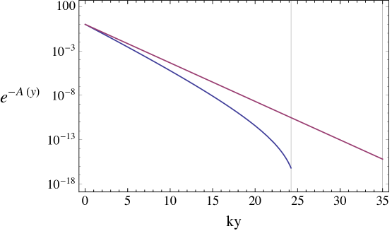
Figure 1: Value of the warp factor as a function of the length along the extra dimension (in units of $k$) for both the RS (linear plot in pink) and for the $MAdS_{5}$ (curved plot in blue) scenarios.

In Fig. 1 we show the value of the warp factor as a function of the length along the extra dimension (in units of $k$) for both the RS (in pink) and for the $MAdS_{5}$ (in blue) scenarios showing how, in the $MAdS_{5}$ case, one produces the Planck-TeV hierarchy with a shorter extra-dimensional length due to stronger warping near the TeV boundary.

The bulk Higgs mass is given by

$$M^{2}_{H}=a(a-4)k^{2}\left(1-{4\over(a-4)k\Delta\nu^{2}}\right),$$ (7)

yields the following equation of motion for the Higgs profile

$$-\partial_{y}\left(e^{-4A(y)}\partial_{y}h(y)\right)+M^{2}_{H}e^{-4A(y)}h(y)-\lambda^{2}e^{-2A(y)}h(y)=0.$$ (8)

Here $a\in\mathbb{R}$ is the bulk mass parameter of the Higgs field. This parameter determines the localization of the Higgs profile along the extra dimension. For values of $a\gtrsim 10$, the Higgs field is localized on the IR brane and it can effectively be described via a Dirac delta function (Frank:2013un ; Azatov:2010pf ). At the lower limit, $a_{min}$, the Higgs field will be as delocalized as possible while still offering a solution to the hierarchy problem, as explained below.

Introducing the boundary condition as $(\partial_{y}-M_{0})h(y)|_{UV}=0$, the solution to the equation of motion for the Higgs profile can be written as

$$h(y)=h_{0}e^{aky}\bigg{[}1+(M_{0}/k-a)\left[F(y)-F(0)\right]\bigg{]},$$ (9)

where $h_{0}$ is a normalization factor and $M_{0}$ is the brane Higgs mass term (the coefficient of the Higgs boundary potential $|H|^{2}\delta(y-y_{1})$ at the IR brane) introduced to give rise to the Higgs zero mode field with the correct physical mass. The function $F(y)$ is given by

$$F(y)=e^{-2(a-2)ky_{s}}ky_{s}\left[-2(a-2)ky_{s}\right]^{-1+4/\nu^{2}}\Gamma\left[1-\frac{4}{\nu^{2}},-2(a-2)k(y_{s}-y)\right].$$ (10)

As seen from the Higgs profile, Eq. (9), only the first term, $h=h_{0}e^{aky}$ can address the hierarchy problem of the SM. The second term, which is peaked at the UV brane, corresponding to an elementary Higgs field, must be subdominant in order to preserve localization of the Higgs field near the IR brane. One could fine tune $M_{0}/k\simeq a$, but in order to avoid this fine-tuning of the boundary mass term, demanding that

$$\delta\equiv|F(y_{1})|\sim{\cal O}(1),$$ (11)

would be sufficient, as $F(y)$ is a monotonically increasing function. In the following we set $\delta\simeq 0.1-1$ to ensure that we do not introduce a new fine-tuning to the setup.

Once the Higgs vacuum expectation value (VEV) profile is set, the lightest KK mode in the Higgs sector will be identified as the SM Higgs boson, with a mass of 125 GeV. In general terms, one expects the mass of all KK modes to be of similar order, i.e. TeV size. In order to generate a mass 10-20 times lighter one must require some $1-10\%$ tuning of parameters in the scalar sector in order to address this small hierarchy and one should also include all possible quantum corrections to the tree level KK Higgs mass. As long as $\delta\simeq 0.1-1$, this small tuning in the Higgs sector will just be a reflection of the remnant hierarchy between the TeV scale and the electroweak scale, far less worrisome than the Planck-electroweak hierarchy.

Furthermore, it is not obvious that the lightest scalar field in the model should be the Higgs boson. After all, the scenario makes use of a 5D scalar singlet, whose perturbations, mixed with the graviscalar perturbations would generate also a tower of new scalar fields. The lightest one of them, identified as the radion/dilaton could be light, although the expectation is that the strong deviation from $AdS_{5}$ should lift its mass to more generic values of KK fields, i.e. TeV range. This was addressed in Cabrer:2011fb and found dilaton masses consistently growing with the level of deviation from $AdS_{5}$. Finally, it is more than possible that the dilaton tower could mix with the Higgs tower, so that the lightest scalar field in the mixed scalar sector would be some mixture of 5D Higgs, graviscalar and 5D scalar singlet. We will work under the assumption that the graviscalar/5D-singlet tower mixes minimally with the lightest Higgs, so that this last one remains Standard-Model-like (as preferred by experimental data). The next and heavier scalar excitations can still be highly mixed states inheriting Higgs-like, radion-like or sterile couplings but any further study of this sector is beyond the scope of this work.

What makes the model presented in Eq. (4) so interesting is the fact that it substantially alleviates the bounds on the KK masses due to the electroweak precision parameters Cabrer:2011fb . The parameters that introduce the tightest bounds on the $M_{KK}$ are $T$ and $S$ parameters which are given by

$$T = {1\over\alpha}s_{W}^{2}m_{Z}^{2}y_{1}\int e^{2A(y)}(\Omega_{f}-\Omega_{h})^{2}$$ (12)

$$S = {8\over\alpha}s_{W}^{2}c_{W}^{2}m_{Z}^{2}y_{1}\int e^{2A(y)}(\Omega_{f}-y/y_{1})(\Omega_{f}-\Omega_{h}),$$ (13)

where the functions $\Omega_{s}$ for the scalar and $\Omega_{f}$ for the fermion fields are given by

$$\Omega_{h}(y)=\int_{0}^{y}e^{-2A(y)}h^{2}(y)$$ (14)

$$\Omega_{f}(y)=\int_{0}^{y}e^{-3A(y)}f^{2}(y),$$

with $h(y)$ and $f(y)$ the zero mode profiles of the scalar and fermion fields. The functions $\Omega$ have the property that $\Omega_{h}(0)=0$ and $\Omega_{f}(y_{1})=1$. For a UV localized field (i.e. light fermions and gravitons), $\Omega_{f}(y)=1$. Substituting the zero mode profiles of the fields Frank:2013qma , we get

$$\Omega_{h}(y) = {\Gamma(1+2/\nu^{2},2(a-1)ky_{s})-\Gamma(1+2/\nu^{2},2(a-1)k\Delta)\over\Gamma(1+2/\nu^{2},2(a-1)ky_{s})-\Gamma(1+2/\nu^{2},2(a-1)k\Delta_{1})}$$ (15)

$$\Omega_{f}(y) = {\Gamma(1-(1-2c)/\nu^{2},(1-2c)ky_{s})-\Gamma(1-(1-2c)/\nu^{2},(1-2c)k\Delta)\over\Gamma(1-(1-2c)/\nu^{2},(1-2c)ky_{s})-\Gamma(1-(1-2c)/\nu^{2},(1-2c)k\Delta_{1})}$$ (16)

where $k\Delta_{1}\equiv k(y_{s}-y_{1})$. Experimentally the $S$ and $T$ parameters are found Agashe:2014kda

$$S=0.00^{+0.11}_{-0.10},$$ (17)

$$T=0.02^{+0.11}_{-0.12}.$$ (18)

In Fig. 2 we show the bounds that the $S$ and $T$ ranges impose on the parameter region (expressed as KK mass scale $m_{KK}$) of the $MAdS_{5}$ model, with the curvature radius in units of $k$, at the IR brane, $kL_{1}\equiv kL(y_{1})=0.2$. We have only considered the case for UV localized fermion interactions, where $\Omega_{f}=1$. A full analysis of the parameter space of this model is available in Cabrer:2011fb . The left panel of Fig. 2 shows the dependence of the mass scales with the $\nu$ parameter. In generating each point we fixed $kL_{1}=0.2$ and (for the right panel) $\nu=0.5$, which in turn fixes the value for $k\Delta$, given by considering the positive solution to $kL(k\Delta,\nu)=kL_{1}$. With $k\Delta$ given, we obtain the bulk Higgs parameter, $a$, and the position of the IR brane, $y_{1}$ through finding the simultaneous solutions to $\delta(y_{1},\nu,k\Delta,a)=0.1$ and for either the $T(y_{1},\nu,k\Delta,a)$ or the $S(y_{1},\nu,k\Delta,a)$ parameter which satisfies the bounds given by Eq. (17).

Figure 2: Electroweak precision test bounds on the KK masses as functions of the modified metric parameter $\nu$ (left panel) and of the Higgs localization parameter $a$ (right panel), obtained by restricting $\Delta S=(-0.1,0.11),~{}\Delta T=(-0.12,0.11)$.

As it is evident from the figure, the scale of the IR brane (or $m_{KK}$) is determined by $A(y_{1})$ which in turn is related to the volume of the extra dimension. The figure also shows that the values of $kL_{1}=0.2$ and $\nu=1/2$ result in best bounds on the KK masses, which can be as low as $\sim 700$ GeV. It turns out that after considering all possible values of $kL_{1}$, and scanning the parameter space of these models, this region still provides the most relaxed constraints on the KK masses. For this reason, in our numerical analysis provided in the next sections, we use this parameter space and contrast it to the RS regime, given by taking the limits $\nu\rightarrow\infty$ and $y_{s}\rightarrow\infty$. Note that the latter corresponds to bounds on $m_{KK}$ of order 10 TeV Huber:2000fh .

It is also worth noting that the localization of the Higgs field has also an important effect on the bounds shown in Fig. 2. The lowest value of $a$ that we consider is $a_{min}$, defined as the value of the $a$-parameter such that $\delta=0.1$, and therefore such that any value of $a\geq a_{min}$ will require no fine-tuning in order to solve the gauge hierarchy problem. In the same figure, we show the relationship between the $a$ parameter and the lowest allowed KK mass, $m_{KK}$. As one can see from the figure, higher $a$ parameter values introduce tighter bounds on the KK masses from the electroweak precision test constraints.

III Fermion Yukawa Couplings and $gg\to h$ cross section

In this section we present the numerical calculations for the $hgg$ couplings considering the full flavor structure of the SM. We present our results for two cases, first for the choice $\{kL(y_{1}),\nu\}=\{0.2,0.5\}$, which corresponds to the parameter region where electroweak precision constraints are the smallest, and then in the limit $\{kL(y_{1}),\nu\}=\{0.9999,10\}$ which corresponds to the RS regime. In order to compare the two scenarios we set the value of $A(y_{1})$ in each case such that the lightest KK masses are about $2-2.5$ TeV. Having fixed $kL_{1},~{}\nu$ and $A(y_{1})$, we solve for $y_{1}$ and $y_{s}$ from Eqs. (4) and (5). We also obtain the value for $a_{min}$ (the lowest Higgs field localization mass parameter) by requiring that $\delta(y_{1},a)=0.1$, see Eq. (11). Due to the costly computational procedure, for the numerical results in this paper we only consider $a$ such that $a\in\{a_{min},a_{min}+0.5,a_{min}+1,\dots,a_{max}<6.5\}$. With the background metric parameters fixed, we then construct a fully realistic model which reproduces all  the SM masses and mixing angles. For this we scan over random anarchic fermion bulk mass parameters, (i.e., $c$-parameters) and the 5D Yukawa couplings (we consider two situations, first the case where the Yukawa couplings are of order $\sim 1$ and then when they are of order $\sim 3$).

Using these values for $Y_{5D}$’s and $c$’s, and only considering the zero mode profiles for which analytic expressions are available, we construct the $3\times 3$ Yukawa coupling matrix with the following elements

$$(y^{0}_{u})_{ij}=\frac{(Y^{5D}_{u})_{ij}}{\sqrt{k}}\int_{0}^{y_{1}}dye^{-4A(y)}h(y)q^{0,i}_{L}(y)u^{0,j}_{R}(y)\,,$$ (19)

where $(Y^{5D}_{u})_{ij}$ are the 5D dimensionless Yukawa couplings and $u\in\{u,d\}$ for up and down quarks, and $q^{0,i}_{L}(y)$ and $u^{0,j}_{R}(y)$ are the $SU(2)$ doublet and singlet zero mode quark wave functions (the SM quarks) in the gauge basis, obtained in the limit when the Higgs vacuum expectation value (VEV) $v\to 0$.

When the previous Yukawa matrix reproduces well enough the SM masses and mixings, we construct the first 2 KK (and later we repeat for 3 KK) profiles for fermions by solving numerically the differential equations for the equations of motions of the fermion profiles for all 6 flavors (in the gauge basis and in the limit $v\to 0$):

$$\partial_{y}\left(e^{(2c-1)A(y)}\partial_{y}\left(e^{-(c+2)A(y)}\right)\right)f(y)+e^{(c-1)A(y)}\lambda^{2}f(y)=0,$$ (20)

with Dirichlet boundary conditions for the “wrong” chirality fermions. Equipped with the KK profiles, we compute all Yukawa couplings in the setup with $N$ complete KK levels, and construct the Yukawa matrix of dimension $(3+6N)$, i.e. $15\times 15$ when the number of KK levels is $N=2$, and $21\times 21$ when the KK levels are $N=3$. We write, for the up sector

$${\bf Y}_{u}=\left(\begin{array}[]{ccc}(y^{0}_{u})_{3\times 3}&(0)_{3\times 3N}&(Y^{qU})_{3\times 3N}\\ (Y^{Qu})_{3N\times 3}&(0)_{3N\times 3N}&(Y_{1})_{3N\times 3N}\\ (0)_{3N\times 3}&(Y_{2})_{3N\times 3N}&(0)_{3N\times 3N}\end{array}\right),$$ (21)

with the down sector Yukawa matrix ${\bf Y}_{d}$ computed in the same way. The submatrices are obtained by the overlap integrals

$$Y^{qU}=\frac{Y^{5D}_{ij}}{\sqrt{k}}\int_{0}^{y_{1}}dye^{-4A(y)}h(y)q^{0,i}_{L}(y)U^{n,j}_{R}(y)$$ (22)

$$Y^{Qu}=\frac{Y^{5D}_{ij}}{\sqrt{k}}\int_{0}^{y_{1}}dye^{-4A(y)}h(y)Q^{m,i}_{L}(y)u^{0,j}_{R}(y)$$ (23)

$$Y_{1}=\frac{Y^{5D}_{ij}}{\sqrt{k}}\int_{0}^{y_{1}}dye^{-4A(y)}h(y)Q^{m,i}_{L}(y)U^{n,j}_{R}(y)$$ (24)

$$Y_{2}=\frac{Y^{5D}_{ij}}{\sqrt{k}}\int_{0}^{y_{1}}dye^{-4A(y)}h(y)Q^{m,i}_{R}(y)U^{n,j}_{L}(y)\,,$$ (25)

where the indices $m$ and $n$ track the KK level and $i$ and $j$ are flavor indices. The corresponding fermion mass matrix ${\bf M}_{u}$, of dimension $(3+6N)$, is given by

$${\bf M}_{u}=\left(\begin{matrix}vy^{0}_{u}&0&vY^{qU}\\ vY^{Qu}&M_{Q}&vY_{1}\\ 0&vY_{2}&M_{U}\end{matrix}\right)$$ (26)

where $M_{Q}$ and $M_{U}$ are the $3N\times 3N$ diagonal KK mass matrices and where $v=174$ GeV. We construct a similar mass matrix ${\bf M}_{d}$ for the down sector.

We now have to redefine fields to go to the mass basis by diagonalizing ${\bf M}_{u}$ through the bi-unitary transformation

$${\bf M}_{u}\rightarrow V_{L}{\bf M}_{u}V_{R}.$$ (27)

The same transformation has to be applied to the Yukawa matrix as well

$${\bf Y}_{u}\rightarrow V_{L}{\bf Y}_{u}V_{R}.$$ (28)

Note that the transformed ${\bf Y}^{phys}_{u}$ matrix by this procedure is not necessarily diagonal. Also note that at this point, due to the contribution of the tower of KK modes, the naive 0-mode masses and CKM mixings which where arrived at through our first scan, might have been significantly shifted. This amount of this shift depends on the value of the $a$-parameter, and is most significant for the top quark mass. Following a try and error method, we go back to the first step and redo the scanning and refine our screening to find the $c$-parameters and 5D Yukawa couplings such that these final masses and CKM mixing angles, which include mixing with the KK tower of fermions, are realistic.

The dominant contribution to the $hgg$ coupling is obtained at one-loop level by calculating the diagram shown in Fig. 3, with fermions running in the loop. The diagram yields a cross section equal to Gunion:1989we

$$\sigma_{gg\rightarrow h}={\alpha_{s}^{2}m_{h}^{2}\over 576\pi}(c^{S}_{ggh})^{2}\ \delta(\hat{s}-m_{h}^{2}),\ \ \ {\rm with}\ \ \ \ c^{S}_{ggh}=\sum_{f}{Y_{f}\over M_{f}}A^{S}_{1/2}(\tau_{f}),$$ (29)

where $Y_{f}$ are the diagonal entries of the fermion Yukawa matrix in the physical basis ${\bf Y}^{phys}_{u}$, and $M_{f}$ are the diagonal entries in ${\bf M}^{phys}_{u}$. In the case where we keep 2 full KK levels ($N=2$) there are $30$ fermions in the loop (15 up-type and 15 down-type), while for $N=3$, there will be $42$ fermions in the loop, including in both cases the 6 SM quarks.

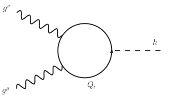
Figure 3: Feynman diagram for the production cross section $gg\to h$ in warped space models.

Here $\hat{s}$ is the invariant momentum squared of the gluons, $\tau_{f}\equiv m_{h}^{2}/4m_{f}^{2}$ and $A^{S}_{1/2}(\tau)$ is the spin-${1\over 2}$ form factor, given by

$$A^{S}_{1/2}(\tau)={3\over 2}\left[\tau+(\tau-1)f(\tau)\right]\tau^{-2},\ \ \ f(\tau)=\left\{\begin{tabular}[]{cc}$\left[\arcsin\sqrt{\tau}\right]^{2}$&$(\tau\leq 1)$\\ $-{1\over 4}\left[\ln\left({1+\sqrt{1-\tau^{-1}}\over 1-\sqrt{1-\tau^{-1}}}\right)-i\pi\right]^{2}$&$(\tau>1)$\end{tabular}\right.$$ (32)

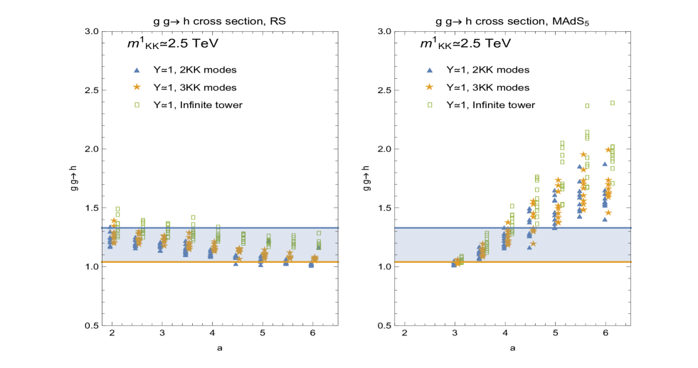
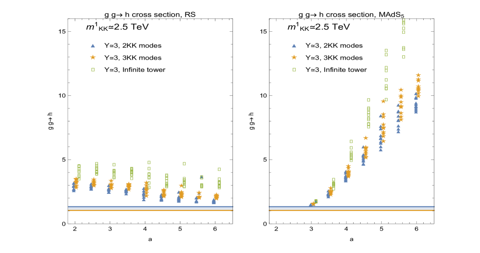
Figure 4: Higgs production rate ratio to Standard Model prediction as a function of the Higgs localization parameter, $a$. We consider an effective theory consisting of a tower of 2 (blue triangles) or 3 (orange stars) KK modes. We also include the results for an infinite tower of KK states (green squares). The KK masses are about $2.5$ TeV in both the RS metric (left panels) and $MAdS_{5}$ scenario (right panels), for which we have chosen $\nu=0.5$, $kL_{1}\simeq 0.2$. The 5D Yukawa couplings are chosen such that $Y^{5D}\sim 1$ (upper panels) and $Y^{5D}\sim 3$ (lower panels). The shaded regions show the experimental bounds from CMS and ATLAS.

In Fig. 4 we plot the Higgs production cross section through gluon fusion. We show on the right panels, the full flavor $gg\rightarrow h$ cross section in the modified $AdS_{5}$ ($MAdS_{5}$) metrics, and on the left side panels we show the results for the same cross section for the model in the RS limit. The top panels are for 5D Yukawa couplings such that $Y^{5D}\sim 1$ and the bottom ones are for $Y^{5D}\sim 3$. Note that in order to generate the top quark mass correctly, the $(Y_{u}^{5D})_{33}$ entry of $Y_{u}^{5D}$ must always be of order $\sim 3$, even when the rest of entries are taken to be $\sim 1$.

As the graphs indicate, the gluon fusion cross section is enhanced compared to the SM one for both models, whether calculated with 2 or 3 or infinite KK levels (see Sec. V for this last case). This confirms the expectation from brane and bulk Higgs production with one flavor Azatov:2010pf ; Frank:2013un and the results from summing over the infinite tower with a bulk Higgs in Archer:2014jca .

Note that in all panels of the graphs, the results obtained using a finite number of KK levels and the results obtained with the complete tower of KK levels start to deviate for larger values of $a$. This is consistent with the findings in Frank:2013un and it is linked to an increased UV sensitivity of the scenario (i.e the decoupling of heavy quark KK modes becomes harder and harder as the Higgs approaches the IR brane). Also note that when the Yukawa couplings become larger, $Y^{5D}\sim 3$, the predictions from the finite KK level calculation and from the infinite KK levels also start to differ (signaling a potential issue). This result is again not surprising since our calculation of the infinite tower relies on the smallness of a perturbative parameter $Y^{2}/M^{2}_{KK}$. As the Yukawa couplings are taken larger and larger, the perturbative calculation becomes worse, and this added to the effect of including the full flavor structure which also increases the size of the perturbations, as 3 families of quarks are now included for each KK level. Even though this might seem as just a calculation problem, we must be aware that we will be quickly approaching a non perturbative limit of the theory, as the Yukawa couplings become strong (i.e. loops including these couplings will start to become comparable to the tree level). Note that in the RS limit, the limit of low values the KK masses is in conflict with electroweak precision bounds, so that for slightly larger KK masses, one could allow for slightly higher Yukawa couplings. In the $MAdS_{5}$, strong coupling limit effects will become rapidly important as the value of the Higgs parameter $a$ grows, since all the Higgs couplings grow exponentially in that limit.

The message from these investigations is therefore that a safe region of parameter space (minimum UV sensitivity and safe from non-perturbative couplings) requires moderate Yukawa couplings $Y^{5D}\sim 1$, as well as low Higgs localization parameter values, $a\sim 2-5$. As the graphs show, in this region both RS and $MAdS_{5}$ seem to be consistent with LHC Higgs production data (except that in the RS limit scenarios are in trouble with flavor and electroweak precision data for these low KK masses).

In Figs. 5 and 6 we have plotted the deviation of the physical top Yukawa coupling with respect to its SM value, and the same for the bottom quark and the tau lepton Yukawa couplings. Again the $MAdS_{5}$ metric scenario is shown on the right side and the RS limit on the left. The consistency between the results of the different calculations (2 KK vs. 3 KK vs. full KK tower) is better here than for the loop-dominated graphs in which all families of KK quarks contributed evenly to the results (essentially as a trace), whereas for single SM quark coupling essentially only one KK tower contributes.

Although their effect to the gluon fusion cross section is not as important as that of the top quark, measurements of the $hb\bar{b}$ and $h\tau^{+}\tau^{-}$ are underway, and higher precision at the Run II of the LHC means that these could be compared to the experimental data in the near future.

Finally in Fig. 7 we show a comparison between the top Yukawa couplings and the gluon fusion cross section in $MAdS_{5}$ (right) and the corresponding RS limit (left). In the figure, the values for $a$ parameter decrease from left to right along the diagonal in both plots. The SM values, shown as black blobs are indicted in the bottom right-hand corner of the plots and appear to overlap with most of the $Y\simeq 1$ parameter points, more so for the $MAdS_{5}$ scenario. The enhancements compared to the SM come mostly from the KK loop-enhanced gluon fusion, as explained above.

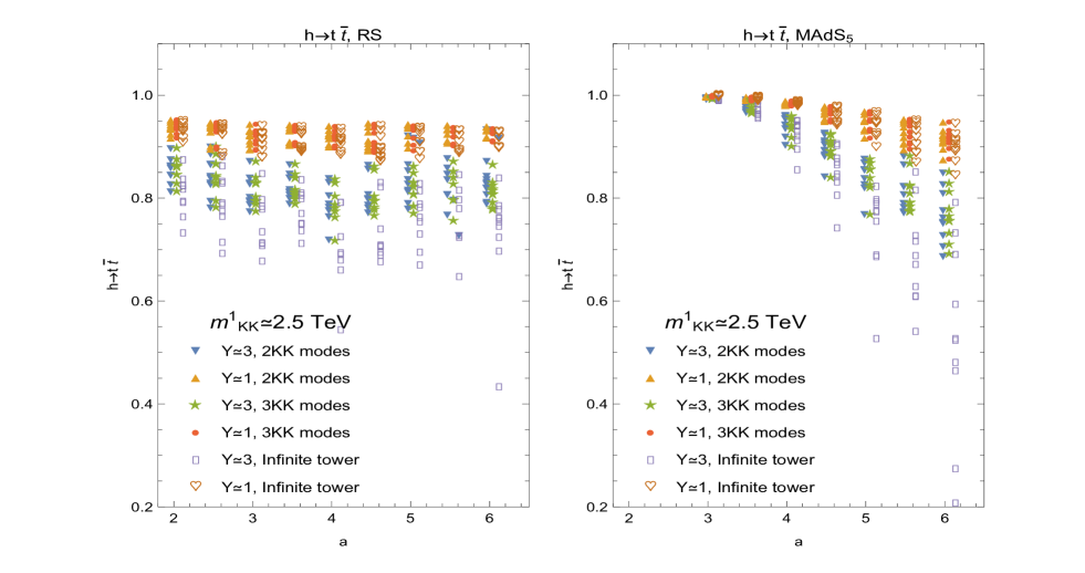
Figure 5: Top quark Yukawa couplings relative to their SM values as a function of the Higgs localization parameter, $a$, in the $MAdS_{5}$ scenario (right), and its RS limit (left). We have considered an effective field theory consisting of a tower of 2 (triangles) and 3 (stars and dots) KK levels with $Y^{5D}\sim 1$ (warm colors) and $Y^{5D}\sim 3$ (cold colors), with the lightest KK mass at about $2.5$ TeV. For both graphs we include also an infinite tower of KK states (hollow shapes). For the general metric scenario, we have chosen $\nu=0.5$, $kL_{1}\simeq 0.2$.

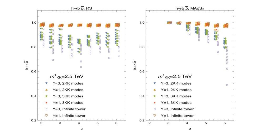
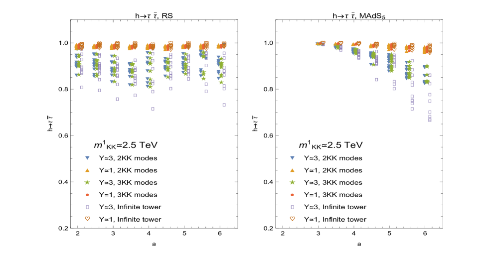
Figure 6: Bottom quark Yukawa couplings (upper panels) and tau lepton Yukawa couplings (lower panels), relative to their SM values, as functions of the Higgs localization parameter, $a$, in the $MAdS_{5}$ scenario (right), and its RS limit (left). We considered a tower of 2 (triangles), 3 (dots and stars) KK modes and an infinite KK tower (hollow shapes).

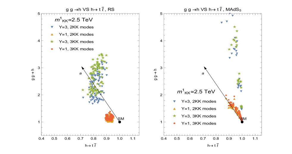
Figure 7: Comparison of the production cross section $gg\to h$ versus the Yukawa couplings for the top quark in $MAdS_{5}$ (right) and the corresponding RS limit (left) a tower of 2 (triangles), 3 (dots and stars) KK modes. The value of the $a$ parameter decreases in both plots, from left to right along the diagonal.

For the plots in Fig. 7 we have set the 5D Yukawa couplings, $Y^{5D}\sim 1$, and considered two models, the $MAdS_{5}$ model and its pure $AdS_{5}$ limit, i.e. RS. Our generic metric model has metric parameters such that $\nu=0.5$, $ky_{1}=0.2$, and KK masses $m_{KK}\sim 2.5$ TeV. For the RS limit, we have taken $\nu=10$, $ky_{1}=0.9999$ and $m_{KK}\sim 2.5$ TeV.

Our results show that the $MAdS_{5}$ models are more sensitive to the values of the $a$-parameter and, while for small values of the $a$-parameter, i.e. a delocalized Higgs field, the model is in accordance with the current experimental bounds on the Higgs production rate through gluon fusion, for larger values of $a$ the enhancement increases. The shift in the Yukawa couplings also exhibit the same $a$-parameter dependence. This result is consistent with our previous results for one generation Frank:2013qma . Note that the Yukawa couplings for both cases of a top-like fermion and an up-like fermion are suppressed, and the reason for the observed enhancement in the $gg\rightarrow h$ cross section is due to the running of KK modes in the loop of the Feynman diagram in Fig. 3 Azatov:2010pf .

Intuitively, the reason for this dependence on the localization of the Higgs field in the $MAdS_{5}$ models is due to the fact that in these models the volume of the fifth dimension is smaller, as shown in Fig. 1. The deviation from the $AdS_{5}$ near the IR brane results in a more aggressive warping of space near that brane. As a consequence all the KK modes, including KK fermions, are pushed more towards the IR brane, which results in smaller values of the overlap integrals of Eq. (22) for a delocalized Higgs field. On the other hand, for the same reason, as the Higgs field becomes more and more localized on the IR brane, deviations become more substantial for the $MAdS_{5}$ scenario compared to the RS-like limit.

IV $h\to\gamma\gamma$ decay

The diagrams responsible for the decay $h\to\gamma\gamma$ in $MAdS_{5}$ are shown in Fig. 8.

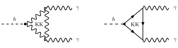
Figure 8: Feynman diagrams for $h\rightarrow\gamma\gamma$ in $MAdS_{5}$.

The decay width from the diagrams, where the KK partners to $W^{\pm}$ bosons run in loop of the left side diagram, and the KK fermions in the right side diagram, respectively, is given by HiggsReview ; Bouchart:2009vq

$$\Gamma_{h\to\gamma\gamma}={{\alpha^{2}m_{h}^{3}}\over{256\pi^{3}}}{1\over{v^{2}}}\left|\sum_{n}{{g^{\pm}_{W^{n}}}\over{m_{W^{n}}^{2}}}A^{h}_{1}(\tau_{W^{n}})+{4\over 3}\sum_{\{f\}}{{Y_{f}}\over{M_{f}}}N_{c}Q_{f}^{2}A^{h}_{1/2}(\tau_{f})\right|^{2},$$ (33)

where $n=\{0,1,2,\dots\}$ for the zero and the corresponding KK modes and $f$ runs over all the fermions and their corresponding KK partners, $N_{c}=3$ for quarks and 1 for leptons, respectively, and $Q_{f}$ is the charge of the fermion in the loop. The form factor $A_{1/2}$ is previously presented in Eq. 32 and for spin-1 bosons in the loop, $A_{1}$, is given by

$$A^{h}_{1}(\tau)=-[2\tau^{2}+3\tau+3(2\tau-1)f(\tau)]\tau^{-2}.$$ (34)

The W boson zero mode and KK masses, $m_{W^{n}}^{2}$ are given by the diagonalization of the mass terms, ${\cal M}^{2}_{\pm}$ in the Lagrangian

$${\cal L}_{\rm mass}^{\rm c}\!=\!(W^{+}_{\mu},W^{+(1)}_{\mu},W^{+(2)}_{\mu}\ \ \dots)\ {\cal M}^{2}_{\pm}\ (W^{-\mu},W^{-(1)\mu},W^{-(2)\mu}\dots)^{T},$$

where the mass matrix and all the gauge boson fields are in the gauge basis. Keeping only the first two KK modes for numerical calculations, we have, in the mass basis

$$\mathcal{M^{\prime}}^{2}_{\pm}\equiv V\ {\cal M}^{2}_{\pm}\ V^{\dagger}={\rm diag}~{}(m^{2}_{W},m^{2}_{W^{1}},m^{2}_{W^{2}}).$$ (35)

Using the transformation as in Eq. (35) to the coupling matrix of the gauge bosons in the gauge basis,

$${\cal L}_{\rm coupling}^{\rm c}\!=2h(W^{+}_{\mu},W^{+(1)}_{\mu},W^{+(2)}_{\mu}\ \dots\ )\ {\cal G}_{\pm}\ (W^{-\mu},W^{-(1)\mu},W^{-(2)\mu}\ \ \dots)^{T},$$ (36)

we obtain

$${\cal L^{\prime}}_{\rm coupling}^{\rm c}\ =\ 2\ h\ (W_{\mu}\ \ W^{1}_{\mu}\ W^{2}_{\mu}\ \ \dots)\ {\cal G^{\prime}}_{\pm}\ (W^{\mu}\ W^{1\mu}\ \ W^{2\mu}\ \ \dots)^{T},$$ (37)

with

$${\cal G^{\prime}}_{\pm}\ =\ V\ {\cal G}_{\pm}\ V^{\dagger}.$$ (38)

The gauge couplings, $g^{\pm}_{W^{n}}$ in Eq. (33) are then given by the diagonal elements of the matrix ${\cal G^{\prime}}_{\pm}$.

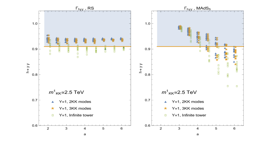
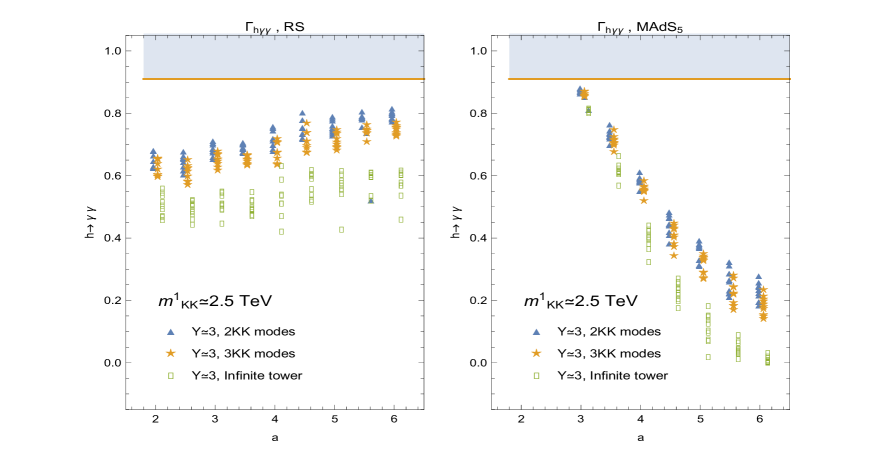
Figure 9: Plot of the decay width for $h\to\gamma\gamma$ in $MAdS_{5}$ relative to SM width, as a function of the Higgs localization parameter, $a$. In all scenarios we consider an effective field theory consisting of a tower of 2 (triangles) or 3 (stars) KK modes. We also include the calculation in which an infinite tower of KK states in included (hollow squares). For the $MAdS_{5}$ (right panels) we have chosen $\nu=0.5$, $kL_{1}\simeq 0.2$. The 5D Yukawa couplings are chosen such that $Y^{5D}\sim 1$ (top panels) and $Y^{5D}\sim 3$ (bottom panels). The left-hand side shows, for comparison, the same values for the RS limit of the model. The lightest KK mass is about $2.5$ TeV in both scenarios.

In Fig. 9 we show the decay width for $h\to\gamma\gamma$ relative to the one in the SM, as a function of the Higgs localization parameter, $a$, for the effective theory containing a tower of 2 (triangles) or 3 (stars) KK modes. We include here, as well, results of the calculation with the infinite KK tower, for the same masses, as explained in the next section, Sec. V, as hollow squares. We plot the values for the $MAdS_{5}$ scenario (right panel) and, for comparison, the same values for the RS limit of the model (left panel). The parameters have been chosen as $\nu=0.5$, $kL_{1}\simeq 0.2$ and the lightest KK mass is about $2.5$ TeV, in both RS and $MAdS_{5}$ scenarios. The 5D Yukawa couplings are chosen such that $Y^{5D}\sim 1$ for the top panels and $Y^{5D}\sim 3$ for the bottom panels. Both models show a suppression of the di-photon decay widths with respect to the SM values, consistent with the one-generation results for RS with fields on the brane in Azatov:2010pf , and for the three-generation in RS with the Higgs field in the bulk in Archer:2014jca . Again, the convergence is better for low $a$ values than for a Higgs localized more towards the brane (larger $a$ values). Note again the discrepancy of the infinite tower calculation in RS limit for $Y=3$ noted in the previous section and linked to approaching a non-perturbative limit for these low KK masses.

Fig. 10 shows the comparison between the loop-dominated production $gg\to h$ and decay $h\to\gamma\gamma$ for the $MAdS_{5}$ model (right panel) and its RS limit (left panel). The correlation function is almost linear for RS. Again the localization parameter $a$ decreases along the diagonal, from left to right and convergence is better for small $a$’s. The $MAdS_{5}$ parameter points overlap with the SM values (solid black circle) for $Y\simeq 1$ (orange region) and even for $Y\simeq 3$, low $a$, while the RS limit has a much smaller region of approximate agreement, and that is only true for $Y\simeq 1$.

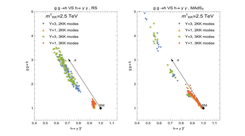
Figure 10: Comparison of the production rate through gluon fusion $gg\to h$ versus the di-photon decay rate in $MAdS_{5}$ for an effective field theory consisting of a tower of 2 (triangles) or 3 (dots and stars) KK modes. The parameters are chosen as in Fig. 9. The SM values are shown for comparison as a black dot. The right panel shows the $MAdS_{5}$ model, compared to the left hand side as RS limit of the model.

V Infinite tower with full flavor contribution

In this section we tackle the calculation of the Higgs couplings when considering the complete towers of KK fields along with the full flavor structure of the SM. The purpose of this exercise is to obtain an independent result from the previous formalism (with two full-flavored KK levels and three full-flavored KK levels) as well as a good check on the decoupling of heavy degrees of freedom in different parts of the parameter space. It is also important to note that the full tower calculation presented here is performed perturbatively (in terms of $Y^{2}v^{2}/M_{KK}^{2}$), so that for larger Yukawa couplings the convergence of the expansion should worsen. We set up the calculation for the up-quark sector, with the understanding that it can be trivially extended for both the down-quark sector and the charged lepton sector.

We introduce a set of three families of 5D $SU(2)$ quark doublets $Q^{i}(x,y)=q_{L}^{i}(x,y)+q_{R}^{i}(x,y)$ with 5D family index $i=1,2,3$, as well as three quark singlets $U^{i}(x,y)=u_{R}^{i}(x,y)+u_{L}^{i}(x,y)$, where $x$ represents the 4D spacetime variables and $y$ the extra dimension. We perform the dimensional reduction as usual, by setting the following separation of variables for the different 5D quark fields:
$\ \ \displaystyle q^{i}_{L}(x,y)=\sum_{n=0}^{3N}q_{L}^{in}(y)\,q_{L}^{n}(x)$, $\ \displaystyle q^{i}_{R}(x,y)=\sum_{n=0}^{3N}q_{R}^{in}(y)u^{n}_{R}(x)$, $\ \displaystyle u^{i}_{L}(x,y)=\sum_{n=0}^{3N}u_{L}^{in}(y)q_{L}^{n}(x)$, and $\ \displaystyle u^{i}_{R}(x,y)=\sum_{n=0}^{3N}u^{in}_{R}(y)\,u_{R}^{n}(x)$.

Note that the $n=0$ states ($q_{L}^{0}(x)$ and $u^{0}_{R}(x)$) are the SM doublet and singlet up-quark, and contain a piece of each of the three bulk families, represented by the twelve wavefunctions $q_{L}^{10}(y)$, $q_{L}^{20}(y)$, $q_{L}^{30}(y)$, $q_{R}^{10}(y)$ etc$\dots$ . Successively, $n=1$ corresponds to the SM charm quark and $n=3$ to the SM top quark, each of them carrying a mixture of twelve wavefunctions. Higher values of $n$ correspond to heavy KK quarks. Within the warped metric background of Eq. (1), the coupled equations of motion corresponding to the 12 wavefunctions for each KK level $n$ are

$$m_{n}^{*}q_{L}^{in}+e^{A+Q_{q_{i}}}\partial_{y}(q_{R}^{in}e^{-2A-Q_{q_{i}}})-e^{-A}v(y)\sum_{j=1}^{3}\frac{Y^{*}_{ij}}{\sqrt{k}}u^{jn}_{R} = 0$$ (39)

$$m_{n}q_{R}^{in}-e^{A-Q_{q_{i}}}\partial_{y}(q_{L}^{in}e^{-2A+Q_{q_{i}}})-e^{-A}v(y)\sum_{j=1}^{3}\frac{Y^{*}_{ij}}{\sqrt{k}}u^{jn}_{L} = 0$$ (40)

$$m_{n}^{*}u_{L}^{in}+e^{A+Q_{u_{i}}}\partial_{y}(u_{R}^{in}e^{-2A-Q_{u_{i}}})-e^{-A}v(y)\sum_{j=1}^{3}\frac{Y_{ji}}{\sqrt{k}}q^{jn}_{R} = 0$$ (41)

$$m_{n}u_{R}^{in}-e^{A-Q_{u_{i}}}\partial_{y}(u_{L}^{in}e^{-2A+Q_{u_{i}}})-e^{-A}v(y)\sum_{j=1}^{3}\frac{Y_{ji}}{\sqrt{k}}q^{jn}_{L} = 0$$ (42)

where we defined

$$Q_{i}(y)\equiv\int M_{i}(y)dy,$$

with $M_{i}(y)$ being the 5D bulk mass associated to each 5D fermion. For simplicity and to maintain an analogy with the usual bulk RS scenario, we take

$$Q_{i}(y)\equiv c_{i}A(y)$$ (43)

with $c_{i}$ being the bulk fermion $c$-parameters similar to the RS ones.

From the previous equations we can obtain the following exact relations for the effective 4D mass $m_{n}$ of the $n$-th KK level as well as its effective 4D diagonal Yukawa coupling $y_{nn}$

$$m_{n} = \sum_{i,j=1}^{3}\int dy\Big{(}e^{-3A}m_{n}\left(u^{in*}_{L}u_{L}^{in}+q_{R}^{in*}q_{R}^{in}\right)+e^{-4A}{v(y)}\left(q_{L}^{in}\frac{Y_{ij}}{\sqrt{k}}u_{R}^{jn*}-q_{R}^{in*}\frac{Y^{*}_{ij}}{\sqrt{k}}u_{L}^{jn}\right)\Big{)}\hskip 28.45274pt$$ (44)

$$y_{nn} = \sum_{i,j=1}^{3}\int dye^{-4A}{h(y)}\left(q_{L}^{in}\frac{Y_{ij}}{\sqrt{k}}u_{R}^{jn*}+u_{L}^{in}\frac{Y^{*}_{ji}}{\sqrt{k}}q_{R}^{jn*}\right)\Big{)}\hskip 28.45274pt\$$ (45)

where $v(y)$ and $h(y)$ are the profiles of the Higgs VEV and of the lowest Higgs KK state (i.e the profile of the SM Higgs field). The shift between the mass term and the diagonal Yukawa term is

$$\Delta_{n}\ =\ m_{n}-v_{4}y_{nn}\ =\ \sum_{i,j=1}^{3}\int dy\Big{(}e^{-3A}m_{n}\left(u^{in*}_{L}u_{L}^{in}+q_{R}^{in*}q_{R}^{in}\right)-2e^{-4A}{v(y)}q_{R}^{in*}\frac{Y^{*}_{ij}}{\sqrt{k}}u_{L}^{jn}\Big{)}$$ (46)

The off-diagonal 4D effective Yukawa coupling between the Higgs boson and two fermions of levels $n$ and $m$ is

$$y_{nm}=\sum_{i,j=1}^{3}\int dye^{-4A}{h(y)}\left(q_{L}^{in}\frac{Y_{ij}}{\sqrt{k}}u_{R}^{jm*}+u_{L}^{in*}\frac{Y^{*}_{ji}}{\sqrt{k}}q_{R}^{jm*}\right)\Big{)}\hskip 28.45274pt\$$ (47)

We can thus calculate these terms if we know the solutions for the profiles from the coupled equations (39), (40), (41) and (42).

The strategy we follow is to solve them perturbatively for the case of light (SM) modes, and therefore obtain masses and Yukawa couplings for the SM up quark, charm quark and top quark, i.e. the levels $n=0,1,2$. We obtain

$$q_{L}^{in}(y) \simeq e^{2A-Q_{q_{i}}}\left(Q_{L}^{in}+m_{n}\int q^{in}_{R}(y)e^{-A+Q_{q_{i}}}-\sum_{j}\frac{Y^{*}_{ij}}{\sqrt{k}}\int e^{-2A+Q_{q_{i}}}v(y)u^{jn}_{L}(y)\right)$$ (48)

$$u_{R}^{in}(y) \simeq e^{2A+Q_{u_{i}}}\left(U_{R}^{in}-m_{n}^{*}\int u^{in}_{L}(y)e^{-A-Q_{u_{i}}}+\sum_{j}\frac{Y_{ji}}{\sqrt{k}}\int e^{-2A-Q_{u_{i}}}v(y)q^{jn}_{R}(y)\right)$$ (49)

$$q_{R}^{in}(y) \simeq e^{2A+Q_{q_{i}}}\left(-Q_{L}^{in}m_{n}^{*}\int_{0}^{y}e^{A-2Q_{q_{i}}}+\sum_{j}\frac{Y_{ij}^{*}}{\sqrt{k}}U_{R}^{jn}\int_{0}^{y}e^{Q_{u_{j}}-Q_{q_{i}}}v(y)\right)$$ (50)

$$u_{L}^{in}(y) \simeq e^{2A-Q_{u_{i}}}\left(U_{R}^{in}m_{n}\int_{0}^{y}e^{A+2Q_{u_{i}}}-\sum_{j}\frac{Y_{ji}}{\sqrt{k}}Q_{L}^{jn}\int_{0}^{y}e^{Q_{u_{j}}-Q_{q_{i}}}v(y)\right),$$ (51)

where the 6 constants of integration $Q_{L}^{in}$ and $U_{R}^{in}$ (with $i=1,2,3$ and with the level $n$ fixed) are obtained after imposing Dirichlet boundary conditions on the appropriate wave functions.

We are now equipped to compute the couplings of the Higgs boson with the SM fermions, including this time the effects of the full tower of KK modes. Using these we can address the Higgs production calculation with full KK towers, with the caveat that it is a perturbative calculation, whose convergence should worsen for larger values of the 5D Yukawa couplings.

The radiative couplings of Higgs to gluons will depend on the physical Yukawa couplings $y_{nn}$ of all the fermions running in the loop and on their physical masses $m_{n}$. The real and imaginary parts of the couplings (scalar and pseudoscalar parts) are associated with different loop functions, $A^{S}_{1/2}$ and $A^{P}_{1/2}$, as they generate the two operators $hG_{\mu\nu}G^{\mu\nu}$ and $hG_{\mu\nu}\tilde{G}^{\mu\nu}$.

The cross section is

$$\sigma_{gg\rightarrow h}={\alpha_{s}^{2}m_{h}^{2}\over 576\pi}\left[|c^{S}_{ggh}|^{2}+|c^{P}_{ggh}|^{2}\right]\$$ (52)

where

$$c^{S}_{ggh}=\sum_{n}\hbox{Re}\left({\frac{y_{nn}}{m_{n}}}\right)A^{S}_{1/2}(\tau_{f})\hskip 17.07182pt{\rm and}\hskip 17.07182ptc^{P}_{ggh}=\sum_{n}{\rm Im}\left(\frac{y_{nn}}{m_{n}}\right)A^{P}_{1/2}(\tau_{f})$$ (53)

with $\ \tau=m^{2}_{h}/4m^{2}_{n}\$, with $A^{H}_{1/2}(\tau)$ defined as in Eq.(32) and with $\displaystyle\ \ A^{H}_{1/2}(\tau)=-f(\tau)\tau^{-2}$ Gunion:1989we .

For heavy KK quarks with masses $m_{n}$ much greater than the Higgs mass $m_{h}$ (i.e. when $\tau$ is very small) the loop functions are essentially constant, as they behave asymptotically as $\displaystyle\lim_{\tau\to 0}A^{S}_{1/2}=1\hskip 5.69046pt\mbox{and}\hskip 5.69046pt\lim_{\tau\to 0}A^{P}_{1/2}=3/2.$ On the other hand, for light quarks (all the SM quarks except top and bottom), the loop functions essentially vanish asymptotically as $\displaystyle\lim_{\tau\to\infty}A^{S}_{1/2}=\lim_{\tau\to\infty}A^{P}_{1/2}=0.$

In those two limits, the amplitudes $c^{S}_{ggh}$ and $c^{P}_{ggh}$ can be written in terms of traces involving the infinite fermion mass and Yukawa matrices of the up and down quark sectors, ${\bf M}_{i}$ and ${\bf Y}_{i}$ with $i=u,d$. Since the trace is basis invariant, we consider the infinite mass matrices in the gauge basis ${\bf M}_{u}$ and ${\bf M}_{d}$ as defined in Eq. (26), but this time for the case $N\to\infty$.

The infinite up-type Yukawa matrix can be obtained as $\displaystyle{\bf Y}_{u}=\frac{\partial{\bf M}_{u}}{\partial v}$, and so the traces we want to evaluate can be written as

$$\sum_{n}\hbox{Re}\left({\frac{y^{u}_{nn}}{m^{u}_{n}}}\right)=\mbox{Tr}(\mathbf{Y}_{u}{\bf M}_{u}^{-1})=\mbox{Tr}(\frac{\partial{\bf M}_{u}}{\partial v}{\bf M}_{u}^{-1})=\frac{1}{\det{{\bf M}_{u}}}\frac{\partial}{\partial v}\left(\det{{\bf M}_{u}}\right)$$ (54)

and for the down-type case

$$\sum_{n}\hbox{Re}\left({\frac{y^{d}_{nn}}{m^{d}_{n}}}\right)=\mbox{Tr}(\mathbf{Y_{d}{M_{d}}^{-1}})=\frac{1}{\det{\bf M_{d}}}\frac{\partial}{\partial v}\left(\det{\bf M_{d}}\right)$$ (55)

We evaluate these traces perturbatively by expanding the determinants in powers of $v^{2}/M_{KK}$ where $M_{KK}$ are the masses of the heavy KK fermion excitations. We obtain

$$c^{S}_{ggh} \simeq v\ \hbox{Re}\Big{[}2\ \mbox{Tr}(\Delta^{u}_{H}+\Delta^{d}_{H})+\mbox{Tr}({y^{0}_{d}}^{-1}\Delta^{u}_{2}+{y^{0}_{d}}^{-1}\Delta^{d}_{2})\Big{]}$$ (56)

$$\ \ +\hbox{Re}\left(\frac{y_{t}}{m_{t}}\right)A^{S}_{1/2}(\tau_{t})+\hbox{Re}\left(\frac{y_{b}}{m_{b}}\right)A^{S}_{1/2}(\tau_{b})$$

and

$$c^{P}_{ggh} \simeq v\ {\rm Im}\Big{[}\Big{(}2\ \mbox{Tr}(\Delta^{u}_{H}+\Delta^{d}_{H})+\mbox{Tr}({y^{0}_{u}}^{-1}\Delta^{u}_{2}+{y^{0}_{d}}^{-1}\Delta^{d}_{2})\Big{]}$$ (57)

$$\ \ +{\rm Im}\left(\frac{y_{t}}{m_{t}}\right)A^{P}_{1/2}(\tau_{t})+{\rm Im}\left(\frac{y_{b}}{m_{b}}\right)A^{P}_{1/2}(\tau_{b})$$

where the top and bottom quarks have been treated separately so as to to compute numerically their associated loop functions $A^{S/P}_{1/2}(\tau_{t})$ and $A^{S/P}_{1/2}(\tau_{b})$, without assuming any limiting value for them. We now have to evaluate numerically all the terms in the previous expressions.

• The terms depending on $\displaystyle\frac{y_{t}}{m_{t}}$ and on $\displaystyle\frac{y_{b}}{m_{b}}$ (the ratio of the physical top Yukawa to its mass, and similarly for the bottom) are obtained numerically using Eq. (45), and the perturbative numerical solutions from Eqs. (48), (49), (50) and (51).

• The terms $\mbox{Tr}({y^{0}_{u}}^{-1}\Delta^{u}_{2}+{y^{0}_{d}}^{-1}\Delta^{d}_{2})$ represent the “kinetic” shift in Yukawa couplings and are highly suppressed, except for the top and bottom quarks, so we rewrite them as

  $$\mbox{Tr}({y^{0}_{u}}^{-1}\Delta^{u}_{2}+{y^{0}_{d}}^{-1}\Delta^{d}_{2})\ =\ \frac{\Delta^{t}_{2}}{y^{t}}+\frac{\Delta^{b}_{2}}{y^{b}}\ =\ \frac{1}{v^{2}}\left(\frac{v^{3}\Delta^{t}_{2}}{m_{t}}+\frac{v^{3}\Delta^{b}_{2}}{m_{b}}\right)$$ (58)

  $$= \frac{1}{v^{2}}\sum_{i=1}^{3}\int dza(z)^{4}\Big{(}u^{i\,t*}_{L}u_{L}^{i\,t}+q_{R}^{i\,t*}q_{R}^{i\,t}+d^{i\,b*}_{L}d_{L}^{i\,b}+q_{R}^{i\,b*}q_{R}^{i\,b}\Big{)}$$

  These terms can be also be obtained using the perturbative numerical solutions from Eqs. (48), (49), (50) and (48).

• Finally, the terms with $\Delta^{u}_{H}$ and $\Delta^{d}_{H}$, can be calculated as

  $$\mbox{Tr}(\Delta^{u}_{H})=\mbox{Tr}(M_{Q}^{-1}Y_{1}M_{U}^{-1}Y_{2})$$

  $$=\sum_{i,j=1}^{3}\frac{Y^{5D}_{ij}}{\sqrt{k}}\frac{Y^{5D^{*}}_{ij}}{\sqrt{k}}\int dydy^{\prime}e^{-4[A(y)+A(y^{\prime})]}h(y)h(y^{\prime})\left(\sum_{n_{i}\geq 1}^{\infty}\frac{Q^{n_{i}}_{L}(y)Q^{n_{i}}_{R}(y^{\prime})}{M_{Q_{n_{i}}}}\right)\!\!\!\left(\sum_{m_{i}\geq 1}^{\infty}\frac{U^{m_{j}}_{R}(y)U^{m_{j}}_{L}(y^{\prime})}{M_{U_{m_{j}}}}\right)\ \ \ \ \$$ (59)

  with the submatrices $M_{U}$, $Y_{2}$, $M_{Q}$ and $Y_{1}$ as defined in (26), and with the down-type term obtained similarly. Here, the wave functions in capital letters $Q^{n_{i}}_{L}(y)$, $Q^{n_{i}}_{R}(y)$, $U^{n_{i}}_{R}(y)$ and $U^{n_{i}}_{L}(y)$ correspond to the KK quarks in the the gauge basis, when $v=0$ (i.e. before electroweak symmetry breaking). The masses $M_{Q_{n_{i}}}$ and $M_{U_{n_{i}}}$ are their corresponding masses (again, before electroweak symmetry breaking). These terms with infinite sums can be calculated numerically after using the closure relations (see for example Frank:2013qma )

  $$\sum_{n=1}^{\infty}{{Q}_{L}^{(n)}(y){Q}_{R}^{(n)}(y^{\prime})\over M_{Q_{n}}}=-e^{Q_{q}(y^{\prime})-Q_{q}(y)}\left[\theta(y^{\prime}-y)-{\int_{0}^{y^{\prime}}e^{A-2Q_{q}}\over\int_{0}^{y_{1}}e^{A-2Q_{q}}}\right],$$ (60)

  $$\sum_{n=1}^{\infty}{{U}_{R}^{(n)}(y){U}_{L}^{(n)}(y^{\prime})\over m_{n}}=e^{Q_{u}(y)-Q_{u}(y^{\prime})}\left[\theta(y^{\prime}-y)-{\int_{0}^{y^{\prime}}e^{A+2Q_{u}}\over\int_{0}^{y_{1}}e^{A+2Q_{u}}}\right].$$ (61)

In the case of the coupling of Higgs to photons, one proceeds in a similar way in order to compute the fermion loops taking care to also add the contribution from charged leptons and appropriately account for the different gauge charges and coupling constant.

VI Conclusions

In this work we analyzed the production and decay rates of a bulk-localized Higgs boson in the context of a general 5-dimensional warped spacetime. Our analysis is concentrated on models with metrics modified from the usual RS model, which can account for low energy electroweak and flavor precision measurements. These models generically predict an enhancement in the Higgs production cross section and a suppression in the fermion Yukawa couplings. Nevertheless these predictions can remain in agreement with the LHC data, while still allowing for a low KK scale, within the LHC Run II reach. In a previous work, we presented an analysis of the Higgs boson production which employed a toy model based on one fermion field propagating in the bulk. We expand our considerations to present a more realistic analysis, which exhibits several new features.

First, our investigations include a careful analysis to account for all three families of quarks and leptons, together with their KK towers. In particular, we start with fermion profiles which satisfy masses and mixing constraints (as given by the CKM and PMNS matrices, respectively). We proceed to perform the calculation for production and decay rates, first by considering the theory an effective theory with a cut-off of 2 KK, then 3 KK modes, to test the convergence properties. Second, we then compare the results with those obtained by including a full tower of KK modes for all fermion families. Careful inclusion of the infinite KK tower, without neglecting the flavor mixing, entails some technicalities, described here in some detail. Third, we include also the di-photon decay, which was not evaluated in our previous toy model, and is calculated in the same way: first by taking into account 2 KK and 3 KK modes, then including the full KK tower. And finally, we compare the results for our model with modified metric to the RS limit (meaning that we assume the same parameters for the RS limit, for a fair comparison, while a realistic evaluation of RS models would have to take into account the fact that the KK scale must be much higher).

Our results are showcased as a function of the Higgs localization parameter. For de-localized Higgs bosons (small localization parameter, indicating a bulk Higgs), results obtained using 2 or 3 KK modes agree with each other and with the infinite sum. Localizing the Higgs closer to the brane enhances the gluon fusion cross section and worsens the agreement, meaning that more KK modes are required for agreement. We have chosen two ranges of values for the 5-dimensional Yukawa coupling: $Y^{5D}\sim 1$ and $Y^{5D}\sim 3$. The later illustrates the disagreement between including finite KK levels and including the full towers, as one quickly reaches the non-perturbativity limit for our chosen (low) KK masses. The behavior of $h\to\gamma\gamma$ has similar features to the gluon fusion production: note that, as expected, the gluon fusion cross section is enhanced, while the di-photon decay is suppressed throughout the parameter space, confirming previous results from the one fermion analysis.

Our analysis is presented with the expectation that the Run II of the LHC will measure Higgs boson properties with a high degree of precision, and as such can put further limits on the parameters of this model, or in fact rule it out. To compare with expected measurements, we have included the top, bottom and tau lepton Yukawa couplings compared with the SM ones. We have chosen the warped model with modified metric as the most promising model of extra dimensions with consequences at low (within LHC reach) scales, preferring it over competing models which include extra custodial symmetries with additional fermions, gauge bosons and Higgs representations. A careful and comprehensive analysis, such as this one, is timely and can serve as a map towards revealing physics beyond the Standard Model.

VII Acknowledgements

We thank NSERC and FRQNT for partial financial support under grant numbers SAP105354 and PRCC-191578.

References

- (1) G. Aad et al. [ATLAS Collaboration], Phys. Lett. B 716, 1 (2012) [arXiv:1207.7214 [hep-ex]].
- (2) S. Chatrchyan et al. [CMS Collaboration], Phys. Lett. B 716, 30 (2012) [arXiv:1207.7235 [hep-ex]].
- (3) L. Randall and R. Sundrum, Phys. Rev. Lett. 83, 4690 (1999) [hep-th/9906064]. L. Randall and R. Sundrum, Phys. Rev. Lett. 83, 3370 (1999) [hep-ph/9905221].
- (4) W. D. Goldberger and M. B. Wise, Phys. Rev. Lett. 83, 4922 (1999); W. D. Goldberger and M. B. Wise, Phys. Lett. B 475, 275 (2000); C. Csaki, J. Erlich, T. J. Hollowood and Y. Shirman, Nucl. Phys. B 581, 309 (2000); C. Csaki, M. Graesser, L. Randall and J. Terning, Phys. Rev. D 62, 045015 (2000); O. DeWolfe, D. Z. Freedman, S. S. Gubser and A. Karch, Phys. Rev. D 62, 046008 (2000); N. Arkani-Hamed, S. Dimopoulos and J. March-Russell, Phys. Rev. D 63, 064020 (2001). Also see: M. Geller, S. Bar-Shalom and A. Soni, Phys. Rev. D 89, no. 9, 095015 (2014).
- (5) H. Davoudiasl, J. L. Hewett and T. G. Rizzo, Phys. Lett. B 473, 43 (2000); S. Chang, J. Hisano, H. Nakano, N. Okada and M. Yamaguchi, Phys. Rev. D 62, 084025 (2000); T. Gherghetta and A. Pomarol, Nucl. Phys. B 586, 141 (2000).
- (6) A. Pomarol, Phys. Lett. B 486, 153 (2000).
- (7) Y. Grossman and M. Neubert, Phys. Lett. B 474, 361 (2000).
- (8) S. Chang, J. Hisano, H. Nakano, N. Okada and M. Yamaguchi, Phys. Rev. D 62, 084025 (2000).
- (9) T. Gherghetta and A. Pomarol, Nucl. Phys. B 586, 141 (2000).
- (10) H. Davoudiasl, J. L. Hewett and T. G. Rizzo, Phys. Rev. D 63, 075004 (2001).
- (11) R. Contino, Y. Nomura and A. Pomarol, Nucl. Phys. B 671, 148 (2003) [hep-ph/0306259].
- (12) C. Csaki, A. Falkowski and A. Weiler, JHEP 0809, 008 (2008) [arXiv:0804.1954 [hep-ph]].
- (13) M. S. Carena, A. Delgado, E. Ponton, T. M. P. Tait and C. E. M. Wagner, Phys. Rev. D 71, 015010 (2005); M. S. Carena, A. Delgado, E. Ponton, T. M. P. Tait and C. E. M. Wagner, Phys. Rev. D 68, 035010 (2003); A. Delgado and A. Falkowski, JHEP 0705, 097 (2007).
- (14) C. Csaki, C. Delaunay, C. Grojean and Y. Grossman, JHEP 0810, 055 (2008).
- (15) K. Agashe, R. Contino, L. Da Rold and A. Pomarol, Phys. Lett. B 641, 62 (2006).
- (16) S. J. Huber, Nucl. Phys. B 666, 269 (2003).
- (17) K. Agashe, G. Perez and A. Soni, Phys. Rev. D 71, 016002 (2005); K. Agashe, A. Delgado, M. J. May and R. Sundrum
- (18) K. Agashe, A. Delgado, M. J. May and R. Sundrum, JHEP 0308 (2003) 050. Also see: B. M. Dillon and S. J. Huber, JHEP 1506, 066 (2015)
- (19) A. Falkowski and M. Perez-Victoria, JHEP 0812, 107 (2008).
- (20) B. Batell, T. Gherghetta and D. Sword, Phys. Rev. D 78, 116011 (2008); T. Gherghetta and D. Sword, Phys. Rev. D 80, 065015 (2009); T. Gherghetta and N. Setzer, Phys. Rev. D 82, 075009 (2010).
- (21) J. A. Cabrer, G. von Gersdorff and M. Quiros, JHEP 1105, 083 (2011); J. A. Cabrer, G. von Gersdorff and M. Quiros, Phys. Lett. B 697, 208 (2011); J. A. Cabrer, G. von Gersdorff and M. Quiros, New J. Phys. 12, 075012 (2010); J. A. Cabrer, G. von Gersdorff and M. Quiros, Phys. Rev. D 84, 035024 (2011); J. A. Cabrer, G. von Gersdorff and M. Quiros, JHEP 1201, 033 (2012).
- (22) A. Carmona, E. Ponton and J. Santiago, JHEP 1110, 137 (2011).
- (23) S. Mert Aybat and J. Santiago, Phys. Rev. D 80, 035005 (2009); A. Delgado and D. Diego, Phys. Rev. D 80, 024030 (2009).
- (24) M. Frank, N. Pourtolami and M. Toharia, Phys. Rev. D 87, 096003 (2013).
- (25) M. Frank, N. Pourtolami and M. Toharia, Phys. Rev. D 89, no. 1, 016012 (2014).
- (26) P. R. Archer, M. Carena, A. Carmona and M. Neubert, JHEP 1501, 060 (2015). Also see: U. K. Dey and T. S. Ray, Phys. Rev. D 93, no. 1, 011901 (2016)
- (27) A. Azatov, M. Toharia and L. Zhu, Phys. Rev. D 82, 056004 (2010); A. Azatov, M. Toharia and L. Zhu, Phys. Rev. D 80, 035016 (2009).
- (28) K. A. Olive et al. [Particle Data Group Collaboration], Chin. Phys. C 38, 090001 (2014).
- (29) S. J. Huber and Q. Shafi, Phys. Rev. D 63 (2001) 045010; S. J. Huber, C. A. Lee and Q. Shafi, Phys. Lett. B 531, 112 (2002); C. Csaki, J. Erlich and J. Terning, Phys. Rev. D 66, 064021 (2002); J. L. Hewett, F. J. Petriello and T. G. Rizzo, JHEP 0209, 030 (2002); G. Burdman, Phys. Rev. D 66, 076003 (2002).
- (30) J. F. Gunion, H. E. Haber, G. L. Kane and S. Dawson, Front. Phys. 80, 1 (2000).
- (31) A. Djouadi, Phys. Rept. 457 (2008) 1, A. Djouadi, Phys. Rept. 459 (2008) 1, J. Gunion, H. Haber, G. Kane, and S. Dawson, The Higgs Hunter’s Guide (Westview press, Boulder, CO, 2000).
- (32) C. Bouchart and G. Moreau, Phys. Rev. D 80, 095022 (2009) [arXiv:0909.4812 [hep-ph]].