Magneto-phonon resonance in photoluminescence excitation spectra of magneto-excitons in GaAs/AlGaAs Superlattices

Abstract

Strong increase in the intensity of the peaks of excited magneto-exciton (ME) states in the photoluminescence excitation (PLE) spectra recorded for the ground heavy-hole magneto-excitons (of the 1sHH type) has been found in a GaAs/AlGaAs superlattice in strong magnetic field B applied normal to the sample layers. While varying B the intensities of the PLE peaks have been measured as functions of energy separation $\Delta E$ between excited ME peaks and the ground state of the system. The resonance profiles have been found to have maxima at $\Delta E_{\mbox{\scriptsize max}}$ close to the energy of the GaAs LO-phonon. However, the value of $\Delta E_{\mbox{\scriptsize max}}$ depends on quantum numbers of the excited ME state. The revealed very low quantum efficiency of the investigated sample allows us to ascribe the observed resonance to the enhancement of the non-radiative magneto-exciton relaxation rate arising due to LO-phonon emission. The presented theoretical model, being in a good agreement with experimental observations, provides a method to extract 1sHH magneto-exciton “in-plane” dispersion from the dependence of $\Delta E_{\mbox{\scriptsize max}}$ on the excited ME state quantum numbers.

PACS numbers: 78.66.Fd, 78.55.Cr, 73.61.Ey

I Introduction

Optical transitions in semiconductor superlattices (SLs) have received great attention recently. In contrast to the quasi two-dimensional (2D) case of quantum wells (QWs), quasi-particles in SLs are not fully confined in the growth direction $\hat{z}$. Moreover, periodicity in the distribution of the materials with different band gaps and elastic constants leads to the formation of minibands in the case of free carriers and excitons ba88 ; iv95 , and the appearance of additional optical and acoustic phonon modes iv95 ; ju84 ; so85 ; ts89 ; me89 ; sap95 ; pu95 . Numerous investigations concerning optical observation of excitons and magnetoexcitons (MEs) in QWs (e.g. see Refs. ba82, ; gr84, ; vi90, ; ba98, ) and in Sls fu94 ; mi97 ; ta97 usually leave aside the questions related to the non-radiative excitonic relaxation. At the same time, non-radiative excitonic transitions such as phonon emission or absorption allow one to probe indirectly the exciton-energy dispersion ${\cal E}(\mbox{\boldmath$k$})$ ($k$ is the exciton wave vector). Furthermore, studies of these processes may provide the only way of the experimental measurement of the excitonic dispersion. Indeed, such a powerful method as the hot-luminescence technique (reported for the first time in Ref. mirl81, ), which was widely used for measurements of the hole band-structure in bulk GaAs  ruf ; kash93 and in GaAs/AlGaAs QWs ruf ; kashzach , is inefficient for the study of the excitonic dispersion. Although excited ME states were observed in hot magneto-luminescence measurements mes90 , such experiments can hardly reveal any information on the function ${\cal E}(\mbox{\boldmath$k$})$. This is because hot-luminescence measurements can only probe excitons in their radiative states, i.e. when $k$ is very small, so that ${\cal E}(\mbox{\boldmath$k$})\approx{\cal E}(0)$.

The theoretical investigations of excitonic dispersion have attracted large efforts ever since Gor’kov and Dzyaloshinskii’s work devoted to three-dimensional ME go68 . Later, 2D ME was studied in the paper by Lerner and Lozovik le80 and also in the works concerning 2D excitons without magnetic field ba82 ; gr84 ; br85 . Exciton dispersion relations in SLs presenting the dependencies ${\cal E}(\mbox{\boldmath$k$})$ where $\mbox{\boldmath$k$}\parallel\hat{z}$ (i. e. minibands) were calculated in Ref. di90, . In parallel, the excitonic binding energy in SLs were studied theoretically and experimentally in Ref. ch87, (see also Refs. chu89, ; ch89, ), and later the binding energies of ground and excited states in SLs were calculated in magnetic and electric fields wh90 ; di91 . It is worth noting that two-dimensionality and strong magnetic fields are the features which usually allow the separation of transverse variables $x$ and $y$ from the longitudinal one $z$ ($\mbox{\boldmath$B$}\parallel\hat{z}$) and in addition permit a simplification of the model for valence band due to the removal of degeneracy ba88 ; iv95 .

The present paper is the result of experimental and theoretical studies on the observation of a resonant behaviour in relaxation of MEs in type-I GaAs/Al_0.3Ga_0.7As SLs in a high magnetic field perpendicular to the SL layers. In our experiments we detected only photoluminescence (PL) signal from the ground heavy hole exciton state 1sHH (we employ the usual notation for 2D exciton states ba98 ; ta97 ) while the energy of the laser excitation was continuously varied in a range of  80 meV above the 1sHH PL peak. At particular magnitudes of magnetic field we have observed very strong resonant increase of intensity of peaks corresponding to the excited ME states in PLE spectra. We interpret this effect as a manifestation of the magneto-phonon resonance when strong relaxation of the excited ME state takes place via longitudinal-optic-(LO-) phonon emission. This occurs when frequency $\omega_{\mbox{\scriptsize LO}}$ is equal to an approximate multiple of the excitonic cyclotron frequency $\omega_{c}$ (a similar effect for free electrons in heterojunctions is reported in Refs.ha89, ; ba91, ; va96, ):

$$\hbar\omega_{\mbox{\scriptsize LO}}=N\hbar\omega_{c},\quad N=1,2,3,...$$

Here $\omega_{c}=eB/\mu c$, where $\mu$ is the reduced excitonic mass for transverse motion in the layer plane. To our best knowledge this is the first observation of the magneto-phonon resonance for excitons.

The effect has been found only in one SL sample of the investigated series of SL structures. According to our measurements, the quantum efficiency of this sample is about two orders of magnitude less than that for the other investigated structures. This fact allows us to treat the considered phenomenon as a feature of the enhanced relaxation of the excited ME states rather than the peculiarity of light absorption.

The observed resonance profiles (i.e. integrated intensity of enhanced PLE peaks as a function of their energy separation $\Delta E$ from the ground state) were found to be rather broad (with half-widths above $5\,$meV) and have strong maxima at $\Delta E_{\mbox{\scriptsize max}}$ dependent on the quantum numbers of excited ME states. These facts indicate that transitions to the ground ME state occur via intermediate non-radiative states of the ground excitonic 1sHH band. The theoretical treatment developed in our report allows us to extract certain information about the exciton energy dependence on “in-plane” wave-vector component $q$ from the experimental data.

After the description of the experimental results in Section II we present the theoretical study of the phenomenon in Section III. Finally, in the discussion of Section IV we demonstrate the comparison of the PLE data with the theoretical results and present dispersion curves for the “transverse” 1sHH band $\epsilon(q)\equiv{\cal E}(\mbox{\boldmath$q$},k_{z}=0)$ extracted from our experiment.

II Experiment

Samples used in our investigations are molecular beam epitaxy grown type-I GaAs/AlGaAs SLs. The structures are not intentionally doped and the flat band regime is realized. All the samples have $L_{w}=8\,$nm wide GaAs QWs, while the width of AlGaAs barrier is varied from sample to sample as $L_{b}=2,3,5,10,20\,$nm. All the SLs consist of 20 periods $d=L_{b}+L_{w}$.

The PLE experiments were performed in a He cryostat with a superconducting magnet providing a magnetic field up to 23 T normal to the SL layers. A technique based on employing optical fibers was used for the sample excitation and collection of the PLE signal. In the geometry of our experiment the incident laser light propagates in the direction close to the normal to the SLs layers. In order to measure the PLE spectra we tuned a double 1 m monochromator slightly lower or directly to the ground heavy-hole exciton photoluminescence (PL) peak and scanned the excitation energy of the Ar⁺-pumped Ti-Sapphire laser. The main features of the PLE spectra remained unchanged when the detection position was moved in the limits of the linewidth around the 1sHH PL peak. PLE of two different polarizations, $\sigma^{+}$ and $\sigma^{-}$, was detected by a cooled GaAs detector in the photon counting regime.

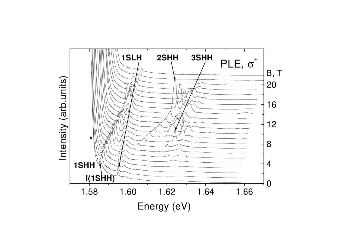
Figure 1: $\sigma^{+}$ PLE spectra recorded for ground magneto-exciton state for various magnetic fields. The excited magneto-exciton peaks are indicated by arrows.

Fig. 1 displays typical heavy-hole exciton PLE spectra for the SL with $L_{w}=8\,$nm and $L_{b}=3\,$nm (referred to as sample 8/3 below) recorded in magnetic field applied normal to the SL layers. We present here the data for $\sigma^{+}$ polarization only, since the observed behaviour is very similar to that for $\sigma^{-}$ polarization. At $B=0$ the most pronounced peaks in the spectrum are the direct heavy hole 1sHH-exciton (its position is not clearly resolved in the shown series of spectra because the laser wavelength was scanned from the high energy side of the 1sHH line), the indirect heavy hole $I$(1sHH)-exciton at $1.586\,$eV  ta97 and the light hole 1sLH-exciton at $1.5955\,$eV  1sHH . When $B$ is increased to 6 T, new features become clearly resolved in the spectra above the 1sLH peak. Energies of these excited states rapidly increase with $B$. The origin of the new peaks can be revealed with the help of an elaborate theoretical analysis of the magneto-exciton band structure. However, this task lies beyond the scope of our investigation. In order to understand the nature of the strongest PLE peaks we carried out a simplified analysis of PLE spectra recorded at high magnetic fields. As a result it has been found that the peaks plotted in Fig. 1 by thick lines correspond to MEs formed by electrons and heavy holes from Landau levels with equal $N=2,3$  (2sHH, 3sHH) ta97 . In what follows we restrict our investigation to the study of the resonant behaviour of these ME states.

As it is seen in Fig. 1, already starting from $B$ of several Teslas the energies of 2sHH and 3sHH ME peaks increase quasi-linearly with $B$. At $B<6\,$T the intensity of the 2sHH ME peak is weak. Then starting from $B=12\,$T the intensity of the 2sHH peak grows rapidly, reaching its maximum at $B=14\,$T and then decreases more slowly. A similar resonant behaviour is clearly observed for the 3sHH ME at $B\approx 9\,$T. Similar resonances have been also observed in $\sigma^{-}$ polarization, however they occur at slightly larger $B$: at $B=17\,$T for 2sHH and at $B=9.5\,$T for 3sHH.

To summarize the PLE data of Fig. 1 (and of the similar series for $\sigma^{-}$) the integrated intensities of the 2sHH and 3sHH MEs are plotted in Figs. 2a,b (black and open squares, respectively) for both polarizations versus the energy separation $\Delta E$ between their positions and the location of the 1sHH peak. The energy of 1sHH peak is extracted from another series of PLE measurements. The variation of $\Delta E$ with increasing magnetic field occurs due to the stronger diamagnetic shifts of the excited ME peaks with respect to that of the 1sHH line (see insets of Figs. 2a,b, where it is seen that $\Delta E$ changes almost linearly with the magnetic field both for 2sHH and 3sHH MEs). Figs. 2a,b show that a very strong increase (by a factor of $10\,-\,20$) of ME peak intensities arises when $\Delta E\approx 35\,$ and $\approx 40\,$ meV for the 2sHH and 3sHH peaks, respectively. These values are very close to the energy of optical phonons in GaAs/AlGaAs  ts89 . Note however that the resonance for the 2sHH peak appears at smaller $\Delta E$ than that for the 3sHH peak. At the same time the resonant enhancement for the 2s$\to$1s transition naturally occurs in stronger magnetic field than the resonance for the 3s$\to$1s one.

The following features of the resonances should be noted as well: (i) their decay as a function of $\Delta E$ is slower than their build-up; (ii) a structure is observed at $\Delta E\approx 37\,$meV for 2sHH ME and at $\Delta E\approx 45\,$meV for 3sHH state.

As it is mentioned above, the precise comparative experiments showed that sample 8/3 had quantum efficiency $\eta$ about two orders of magnitude lower than those of all other SL samples investigated. Meanwhile, other features characterising the quality of the samples such as PL linewidths and Stokes shifts in PLE spectra are very similar for all samples (1.5-2 meV and 1-1.5 meV, respectively). Moreover, the heavy-hole exciton binding energy was found to decrease continuously from the sample with $L_{b}=20\,$nm to the sample with $L_{b}=2\,$nm without any peculiarity for the structure with $L_{b}=3\,$nm  ta97 . These two facts imply that the band structure of sample 8/3 in the energy range close to the energy of the superlattice ground state is as yet unperturbed. We can suppose that strong non-radiative recombination channels are most likely due to deep trapping centers, which originate from native lattice defects defects . However, the nature of non-radiative centers which is caused by growth procedure details of a particular sample plays no significant role in our study.

Closing this Section we would like to note that the intensity of PLE peaks would reflect the absorption efficiency only in the case of $\eta=1$. This condition together with the condition of carriers radiative lifetime being long compared with their relaxation time would permit the excited MEs to relax into the ME ground state without scattering into other states which relax later non-radiatively. On the other hand, in our case of $\eta\ll 1$ the intensity of some peaks can be resonantly enhanced by the mechanism which strongly reduces the relaxation time of the ME transition from the excited state to the radiative ground state and hence decreases to some extent the probability of non-radiative ME escape.

III Theory

III.1 Qualitative consideration of the transition and formulation of the problem

First note that both states, namely initial $|i\rangle$, which is 2sHH or 3sHH, and final $|f_{0}\rangle=$1sHH have very small exciton wave-vectors, since $|i\rangle$ arises by virtue of direct light absorption, whereas $f_{0}$-relaxation directly provides the optical PLE signal. More accurately if $\mbox{\boldmath$q$}=(k_{x},k_{y})$ and $k_{z}$ are the transverse and longitudinal components, then for these states we find for the used experimental geometry that

$$q\lesssim 10^{4}\,\mbox{cm}^{-1},\quad k_{z}\lesssim 10^{5}\,\mbox{cm}^{-1}.$$

Here the right sides are determined by the homogeneity breakdown due to impurities or by momenta of absorbed and emitted photons. Meanwhile the actual extent of the exciton wave functions is of the order of $10\,$nm, since, it is determined by three values: the magnetic length $l_{B}=(c\hbar/eB)^{1/2}$, the effective exciton Bohr radius $a_{B}=\hbar^{2}\varepsilon_{0}/\mu e^{2}$, and the period $d$. In the scale of inverse lengths this reads

$$k_{0}\sim 2\pi/l_{B},2\pi/a_{B},2\pi/d\sim 10^{6}\,-\,10^{7}\,\mbox{cm}^{-1}.$$

The significant difference between the values (3.1) and (3.2) allows one to conclude that the considered resonant transition $i\to f_{0}$ is indirect one. Indeed, due to momentum conservation, in a direct transition the emitted optical phonon would have a negligibly small wave-vector (3.1). As a result the macroscopic LO polarization field applied to ME may be considered to be homogeneous, and in the limit $k/k_{0}\to 0$ the corresponding transition matrix element would be simply proportional to $|\langle i|\mbox{\boldmath$r$}|f_{0}\rangle|$ (with $\mbox{\boldmath$r$}=\mbox{\boldmath$r$}_{2}-\mbox{\boldmath$r$}_{1}$ being the difference between electron and hole positions), which turns out to be equal to zero because of the identical symmetry of the initial and final states with respect to inversion. Thus we consider the LO transition not right into $|f_{0}\rangle$ but initially into $|f\rangle$ which is a 1sHH exciton state with the wave vector $k\sim k_{0}$. Finally, the transition $f\to f_{0}$ is a non-radiative process, e.g. provided by acoustic phonon emission.

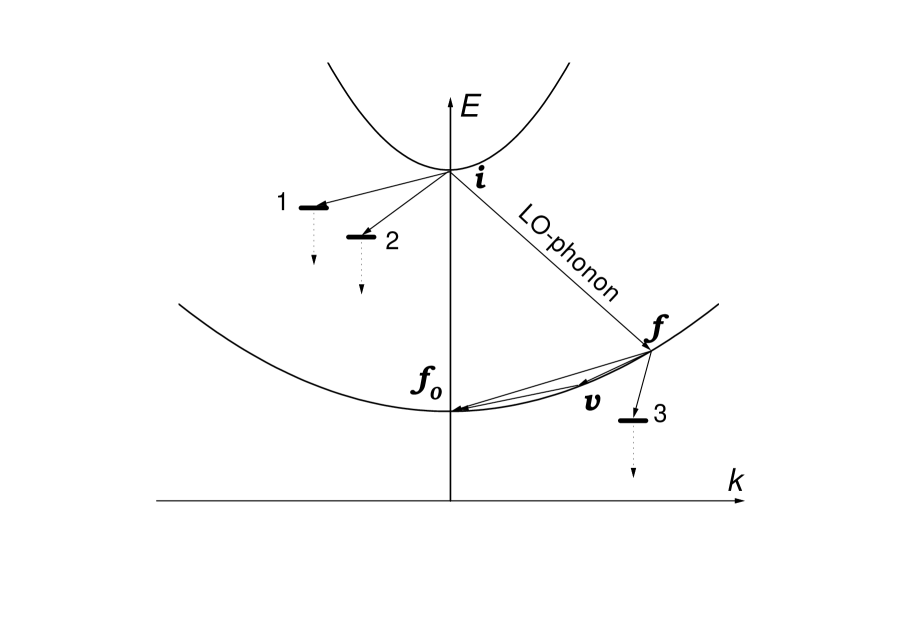
Figure 3: Diagram of possible transitions. LO-phonon-emission $i\to f$ gives rise to the studied effect. Transitions $i\to 1$, $i\to 2$, and $f\to 3$, lead to nonradiative exciton annihilation. Transitions $i\to f\to f_{0}$ and $i\to f\to v\to f_{0}$ are the examples of nonradiative 2(or 3)sHH$\to$1sHH relaxation yielding the measured luminescence signal.

The assumed transitions are schematically demonstrated in Fig. 3. The transitions resulting in non-radiative exciton relaxation are also shown in this diagram. One can see that in the assumed scheme the PLE signal is proportional to the rate of the allowed LO phonon emission.

Among the others the diagram reflects one essential simplification used in our calculations presented below: we ignore the broadening of the exciton peaks, which naturally occurs due to crystal and SL imperfections (the curves in Fig. 3 have zero widths). The diagram implies that $\Delta E=E_{i}-E_{f_{0}}$ should be larger than $\hbar\omega_{\mbox{\scriptsize LO}}$. However, in the experiment the beginning of the enhanced relaxation for 2s-exciton occurs even at $\Delta E\approx 33\,$meV (see Fig. 2), which is lower than the LO phonon energy in a bulk GaAs crystal $\approx 36\,$meV. Here we should note that the value of $\Delta E$ (extracted from PLE spectra) corresponds to the separation of the excited and ground state exciton absorption maxima. Meanwhile the density of states in the vicinity of the ground state is presented by a rather wide band, and at low temperatures the emission comes mostly from the lower states. This fact provides an effective Stokes shift; so that the resonant enhancement of the ground-state luminescence due to LO-phonon mediated relaxation may start at $\Delta E\approx\hbar\omega_{\mbox{\scriptsize LO}}-\Delta_{\mbox{\scriptsize PL}}-\Delta_{\mbox{\scriptsize St}}$, where the PL linewidth $\Delta_{\mbox{\scriptsize PL}}\approx 2\,$meV and the Stokes shift $\Delta_{\mbox{\scriptsize LO}}\approx 1\,$meV. Both values $\Delta_{\mbox{\scriptsize PL}}$ and $\Delta_{\mbox{\scriptsize St}}$ are determined by disorder effects.

In order to describe the data presented in Fig. 2 in the approximation of zero exciton-level width we have to employ an effective energy of LO-phonon which is lower than the tabulated bulk value. As it was described above this disagreement can be easily eliminated by the consideration of the finite exciton peak widths. However, for the simplicity of the model this procedure is omitted in our calculations. The deviation of the LO-phonon energy from the bulk value can also be related to an inevitable effective averaging of the SL multi-mode phonon spectrum in the single-mode approach employed in our model. Later in Sec. IV we will briefly discuss the role of the multi-mode spectrum in the context of the phenomenon studied.

Thus our approach should be considered as a theoretical model, which simplifies the analytical calculation of the relaxation rate as follows:

i) results are obtained in the strong magnetic field approximation, which enables to separate the transverse and longitudinal variables.

ii) we consider only the heavy-hole band ignoring its non-parabolicity and the difference in the effective hole masses in GaAs and Al_0.3Ga_0.7As layers, though we take into account the anisotropy of effective hole mass.

iii) we also ignore the difference of the effective electron masses in GaAs and Al_0.3Ga_0.7As layers.

iv) we consider only one LO-phonon mode with the effective energy $\hbar\omega_{0}=33\,$meV independent of phonon wave-vector direction (to avoid the possible misunderstandings we replace everywhere below $\omega_{\mbox{\scriptsize LO}}$ by $\omega_{0}$). Besides, as in the case of bulk GaAs  gale87 we use only the Fröhlich-type Hamiltonian for electron-LO-phonon as well as for hole-LO-phonon interactions (c.f. Refs. iv95, and na89, ).

v) we ignore possible momentum conservation breakdown and finite widths of the excitonic peaks which occur due to random impurity potential or quantum well and interface roughness.

vi) finally, any spin-orbit terms in the used Hamiltonians are disregarded, therefore the presented theory does not take into consideration the effects of “fine structure” in the PLE signal dependent on light polarization (such effects can be rather peculiar, see e.g. Ref. ba98, ).

In spite of these essential assumptions we believe that such a simplified approach accounts for the most important aspects of the transition shown in Fig. 3 and yields reliable information about the ME relaxation rate.

According to Fig. 3 a considerable enhancement takes place when the intermediate state $|f\rangle$ is a real (not virtual) state of the lowest excitonic band. The general formula for the total probability of the LO phonon emission is

$$W_{\mbox{\scriptsize LO}}=\sum_{f}W_{if}\,,$$

where $W_{if}$ is the probability of the transition into the state $|f\rangle$. Meanwhile subsequent processes of relaxation $f\to f_{0}$ are not the matter of our interest here.

Evidently the energy conservation leads to the equations

$$E_{i}(B)-E_{0}(B)=\hbar\omega_{0}+{\cal E}(\mbox{\boldmath$k$})\,,\qquad E_{f}-E_{0}={\cal E}(\mbox{\boldmath$k$})\,.$$

Here the intermediate exciton state energy is written as $E_{f}=E_{0}+{\cal E}(\mbox{\boldmath$k$})$ where $E_{0}=E_{f_{0}}$ is the ground state energy and ${\cal E}(\mbox{\boldmath$k$})$ is the excitonic kinetic energy. The left side in the first Eq. (3.4) depends quasi-linearly on $B$ (c.f. the insets in Figs. 2a,b) because $E_{i}-E_{0}\equiv N\hbar\omega_{c}+\delta U(B)$, where $\delta U$, being much less than $\hbar\omega_{c}$, is the difference of binding energies in $|i\rangle$ and $|f_{0}\rangle$ states.

At the same time we will see that in strong magnetic field the matrix element for the $i\to f$ transition has a rather sharp maximum in the vicinity of $q=q_{m}\sim l_{B}^{-1}$, which provides really the resonant dependence of PLE signal on the magnetic field.

Let us employ the same material parameters as in Refs. di91, ; di90, , i.e. for the transverse (in the layer of the well) and for the longitudinal hole masses we get $m^{*}_{h\perp}=0.18m_{e}$ and $m^{*}_{h\parallel}=0.34m_{e}$, respectively. The electron mass is $m^{*}_{e\perp}=m^{*}_{e\parallel}=0.067m_{e}$, and the dielectric constant $\varepsilon_{0}$ is equal to 12.5. Then the “transverse” excitonic Bohr radius $a_{0}=\hbar^{2}\varepsilon_{0}/\mu e^{2}$ is $14\,$nm, and for the actual magnetic fields we obtain $l_{B}\leq L_{w}<a_{0}$. This fact justifies the employment of the strong magnetic field approximation: $l_{B}\ll a=\mathop{\rm min}\nolimits{(a_{0},\>L_{w})}$ ($a$ is the characteristic distance between an electron and a hole in ${\hat{z}}$-direction).

The specific dependence ${\cal E}(\mbox{\boldmath$k$})$ is unknown. Nevertheless, the calculations for “free” excitongo68 in a strong magnetic field and for the exciton in SL with $L_{w}=L_{b}$ and $B=0$  di90 make it possible to estimate this value and to find that $\mbox{\footnotesize$\partial$}{\cal E}/{\mbox{\footnotesize$\partial$}q}\sim\mu e^{4}l_{B}^{2}q/\varepsilon_{0}^{2}\hbar^{2}\gg\mbox{\footnotesize$\partial$}{\cal E}/{\mbox{\footnotesize$\partial$}k_{z}}$ Indeed according to Ref. di90, the miniband width for a SL with $L_{w}=L_{b}=3\,$nm is approximately $6\,$meV. Consequently for our SL with the same $L_{b}$ and with $L_{w}=8\,$nm the miniband width should be smaller than $1\,$meV  foot2 . In a strong perpendicular magnetic field this value is to be even more strongly reduced and thus it becomes negligible in comparison with the expected characteristic energy of dependence $\epsilon(q)$.

Further, the summation in Eq. (3.3) leads to the result which contains the density of allowed states $|f\rangle$. This value is inversely proportional to the Jacobian of the change from variables of integration over phase space to the integration over $f$-exciton energy and over $k_{z}$ wave-vector component:

$$\frac{\mbox{\footnotesize$\partial$}({\cal E},\>k_{z})}{\mbox{\footnotesize$\partial$}(q,\>k_{z})}\approx d\epsilon/dq\,.$$

The transition probabilities in Eq. (3.3) are expressed in terms of the relevant matrix element ${\cal M}_{i\to f}$,

$$W_{if}=\frac{2\pi}{\hbar}|{\cal M}_{i\to f}|^{2}\delta(E_{i}-E_{f}-\hbar\omega_{0})\,,$$

which in their turn is calculated using the wave functions of the excitonic states.

III.2 Excitonic wave functions

We can write the excitonic wave functions in the following manner (c.f. Refs. go68, ; le80, ):

$$\Psi(\mbox{\boldmath$r$}_{1},\mbox{\boldmath$r$}_{2},z_{1},z_{2})={\cal L}^{-1}\cdot\exp{\left(i\mbox{\boldmath$R$}\mbox{\boldmath$q$}+\frac{i}{2l_{B}^{2}}[\mbox{\boldmath$r$}_{1}\times\mbox{\boldmath$r$}_{2}]\mbox{\boldmath$B$}/B\right)}\Phi(\mbox{\boldmath$r$}-\mbox{\boldmath$r$}_{0})F(z_{1},z_{2}).$$

Here $j=1,\>2$ denotes electron and hole; $\mbox{\boldmath$r$}_{j}=(x_{j},y_{j})$ is the 2D vector; $\mbox{\boldmath$r$}=\mbox{\boldmath$r$}_{1}-\mbox{\boldmath$r$}_{2},\quad$ $\mbox{\boldmath$R$}=(\mbox{\boldmath$r$}_{1}+\mbox{\boldmath$r$}_{2})/2,\quad$ $\mbox{\boldmath$r$}_{0}=\mbox{\boldmath$B$}\times\mbox{\boldmath$q$}l_{B}^{2}/B;\quad$ ${\cal L}$ is the sample size in the plane $({\hat{x}},\hat{y})$. $\Phi(\mbox{\boldmath$r$})$ obeys two dimensional Srödinger equation in the main approximation of which the Coulomb interaction can be neglected go68 ; le80 . In this case $\Phi(\mbox{\boldmath$r$})\approx|N,m,\mbox{\boldmath$r$}\rangle$ ($N$ is the Landau level number, $m$ is the magnetic quantum number), where

$$|N,m,\mbox{\boldmath$r$}\rangle=\left[\frac{N!}{2^{|m|+1}(N+|m|)!\pi}\right]^{1/2}r^{|m|}l_{B}^{-|m|-1}L_{N}^{|m|}(r^{2}/2l_{B}^{2})e^{im\varphi-r^{2}/4l_{B}^{2}}$$

($L_{N}^{m}$ are Laguerre polynomials). The energies corresponding to these functions are

$$E^{(0)}_{Nm}=\hbar\omega_{c}[N+1/2(|m|+\gamma m+1)],$$

where $\gamma=(m_{h\perp}^{*}-m_{e}^{*})/(m_{h\perp}^{*}+m_{e}^{*})$.

In the next approximation Coulomb interaction can be taken into account with the use of the operator

$${\cal H}_{\mbox{\scriptsize int}}=e^{2}\left/\varepsilon_{0}\sqrt{(\mbox{\boldmath$r$}+\mbox{\boldmath$r$}_{0})^{2}+w^{2}}\right.,\quad\mbox{where}\qquad w=z_{1}-z_{2}\,,$$

in perturbation theorygo68 ; le80 . Coulomb interaction in function $F(z_{1},\,z_{2})$ should be included from the very first step. The Bloch theorem for this function takes place if one changes the variables; namely if

$${\cal F}_{k_{z}}(Z,w)=F(Z+\gamma_{1}w,\;Z-\gamma_{2}w)\,,\quad\mbox{where}\quad\gamma_{1}=m_{h\parallel}^{*}/M,\quad\gamma_{2}=m_{e}^{*}/M\,,$$

then

$${\cal F}_{k_{z}}(Z,w)={\cal L}_{z}^{-1/2}e^{ik_{z}Z}v_{k_{z}}(Z,w)\,,\qquad\mbox{where}\quad v_{k_{z}}(Z+d,w)=v_{k_{z}}(Z,w).$$

(${\cal L}_{z}$ is the sample size along ${\hat{z}}$). We restrict ourselves to the one-band approximation assuming for all $i$ and $f$ states that $v_{k_{z}}(Z,w)$ presents the ground state function of the two-particle motion in $\hat{z}$ direction. This function can evidently be normalized so that $\int_{-\infty}^{+\infty}\int_{Z_{0}}^{Z_{0}+d}|v_{k_{z}}(Z,w)|^{2}dZdw=d$

III.3 Matrix element calculation and inverse transition time

Optical phonons in SLs have considerable energy dependence on their wave-vector direction. Moreover, for arbitrary direction the classification of the optical phonon branches as longitudinal and transverse is impossible due to the inhomogeneity of the superlattice medium along the $z$-axis. We choose the simplified model and calculate ${\cal M}_{i\to f}$ employing the Hamiltonian of exciton-LO-phonon interaction in the following formna89 :

$${\cal H}_{\mbox{\scriptsize opt}}=\frac{1}{{\cal L}}\left(\frac{\hbar}{{\cal L}_{z}}\right)^{1/2}e^{-i\omega_{\mbox{\tiny 0}}t}\sum_{\mbox{\footnotesize{{\boldmath$k$}}}}U_{\mbox{\scriptsize opt}}(\mbox{\boldmath$k$})\left(e^{i{\mbox{\footnotesize{{\boldmath$qr$}${}_{1}$}}}+ik_{z}z_{1}}-e^{i{\mbox{\footnotesize{{\boldmath$qr$}${}_{2}$}}}+ik_{z}z_{2}}\right)+\mbox{H.c.}\,.$$

Final results include only the squared modulus of the vertex, which is

$$|U_{\mbox{\scriptsize opt}}|^{2}=\frac{2\pi e^{2}\omega_{0}}{\overline{\varepsilon}k^{2}}\,.$$

Here ${\overline{\varepsilon}}^{-1}=\varepsilon^{-1}_{\infty}-\varepsilon^{-1}_{0}$ (the standard notationsgale87 are used).

Note that the calculation of $\langle i|{\cal H}_{\mbox{\scriptsize opt}}|f\rangle$ with the functions (3.8) without Coulomb interaction gives exactly zero in the result. Indeed the factorization in the form of the product of one-particle $N$-Landau-level functions is always possible for these functions. Therefore if we are interested in the transition between the different levels $N_{1}$ and $N_{2}$, then the matrix element of a one-particle operator always includes the convolution over the transverse variables $\mbox{\boldmath$r$}_{j}$ of one of the particles $\langle N_{1},m|m,N_{2}\rangle$ which is zero because $N_{1}\not=N_{2}$. Thus ${\cal M}_{i\to f}$ is defined by Coulomb corrections to $\Phi(\mbox{\boldmath$r$})$, which were discussed above. Taking into account this comment, the final expression for the matrix element is

$${\cal M}_{i\to f}=\sum_{v}\frac{\langle v,\mbox{\boldmath$k$}|{}_{\perp}\!\langle f,\mbox{\boldmath$k$}|{\cal H}_{\mbox{\scriptsize int}}|v,\mbox{\boldmath$k$}\rangle\!{}_{\perp}|{\cal H}_{\mbox{\scriptsize opt}}|i,0\rangle}{E_{i}^{(0)}-E_{v}^{(0)}-\hbar\omega_{0}}+\sum_{v}\frac{\langle f,\mbox{\boldmath$k$}|{\cal H}_{\mbox{\scriptsize opt}}|{}_{\perp}\!\langle v,0|{\cal H}_{\mbox{\scriptsize int}}|i,0\rangle\!{}_{\perp}|v,0\rangle}{E_{f}^{(0)}-E_{v}^{(0)}+\hbar\omega_{0}}\,.$$

Here to calculate the expectations one should use the following rules: Brackets ${}_{\perp}\!\langle...,\mbox{\boldmath$k$}|...|...,\mbox{\boldmath$k$}\rangle\!{}_{\perp}$ mean the integration over the transverse variables of Coulomb energy with the functions (3.7); if $\mbox{\boldmath$q$}=0$ then in Eq. (3.9) $\mbox{\boldmath$r$}{}_{0}=0$. Usual brackets $\langle...\rangle$ mean full expectation (the integration over $\mbox{\boldmath$r$}{}_{1},z_{1},\mbox{\boldmath$r$}{}_{2},z_{2}$). Denominators in (3.14) contain the energy values in zero-order approximation in the interaction and hence one should assume that $E_{i}^{(0)}-E_{f}^{(0)}=N\hbar\omega_{c}\approx\hbar\omega_{0}$. Indexes $i$, $v$ $f$ are two-dimensional (each of them is a pair $N,m$). In our case $i=(N,0)$, $f=(0,0)$. The allowed $v$ in the first sum are $(N,\pm m)$ or $[s,\pm(N-s)]$ with $s=0,\,1,...N-1$; and in the second sum $v=(0,0)$. Note also that for $\mbox{\boldmath$q$}=0$ the value (3.14) becomes zero.

After all the integrals are calculated, the matrix element to the first order in $l_{B}/a$ takes the form:

$${\cal M}_{i\to f}=\left(\frac{\hbar}{V}\right)^{1/2}\frac{e^{2}}{\hbar\omega_{c}\varepsilon_{0}}U_{\mbox{\scriptsize opt}}T(k_{z}){\cal G}_{N}(ql_{B})\,,$$

where $V={\cal L}^{2}{\cal L}_{z}$,

$$T(k_{z})=\langle{\cal F}_{k_{z}}(Z,0)|e^{ik_{z}Z}|{\cal F}_{0}(Z,0)\rangle=d^{-1}\int_{Z_{0}}^{Z_{0}+d}v^{*}_{k_{z}}(Z,0)v_{0}(Z,0)\,dZ\;\sim\;\frac{1}{a}\,,$$

$${\cal G}_{1}(p)=-\frac{4\gamma}{1-\gamma^{2}}e^{-p^{2}/4}(1-e^{-p^{2}/2})+\sum_{m=1}^{\infty}\frac{\gamma e^{-3p^{2}/4}mp^{2m}(m+1-p^{2})}{2^{m}(m+1)![(1+m/2)^{2}-m^{2}\gamma^{2}/4]}\,,$$

$${\cal G}_{2}(p)=\frac{-\gamma(1-p^{2})}{1-\gamma^{2}}e^{-p^{2}/4}\left[1-e^{-p^{2}/2}(1+p^{2}/2)\right]-\frac{2\gamma}{9-\gamma^{2}}p^{2}(1+p^{2}/4)e^{-3p^{2}/4}$$

$$+\sum_{m=1}^{\infty}\frac{\gamma me^{-3p^{2}/4}(p^{2}/2)^{m}(m+1-p^{2}/2)\left[m^{2}+3(1-p^{2}/2)(m-p^{2})+2\right]}{2(m+2)!\left[(2+m/2)^{2}-m^{2}\gamma^{2}/4\right]}\,.$$

Now we have to substitute the expression (3.15) into Eq. (3.6). Then in Eq. (3.3) with the help of Eq. (3.5) we change from the summation over states $f$ to the integration over phase space and further to the integration over $\epsilon$ and $k_{z}$. We find then that the $\delta$-function in Eq. (3.6) removes the integration over $\epsilon$. Finally, the result for the total probability of the transition from the excited ME state to some state of the ground ME band is

$$W_{\mbox{\scriptsize LO}}(B)=\frac{e^{6}\omega_{0}\Lambda(q)G_{N}(ql_{B})}{(\hbar\omega_{c})^{2}\varepsilon_{0}^{2}\overline{\varepsilon}d\epsilon/dq}\,,$$

where

$$\Lambda(q)=\frac{q}{\pi}\int_{-\infty}^{-\infty}\frac{|T|^{2}dk_{z}}{q^{2}+k_{z}^{2}}\,,$$

and the functions

$$G_{N}(p)=\pi{\cal G}_{N}^{2}(p)$$

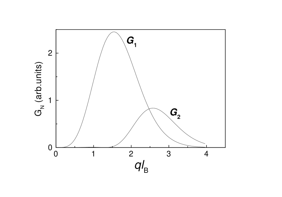
Figure 4: Functions $G_{N}$ versus the dimensionless “in plane” wave-vector component. Landau level numbers $N=1,\,2$ correspond to 2s$\to$1s and 3s$\to$1s transitions respectively.

are plotted in Fig. 4. One should bear in mind that $q$ in Eq. (3.19) is not independent value but $q=q(B)$ is the root of first Eq. (3.4) with ${\cal E}(\mbox{\boldmath$k$})\approx\epsilon(q)$ Therefore $W_{\mbox{\scriptsize LO}}$ is the function of magnetic field which may be converted to the function of $(N+1)$sHH-exciton peak position (see insets in Figs. 2a,b).

Note also that the maximum of function $G_{2}$ is shifted substantially to higher $q$ than that of function $G_{1}$. This fact accounts for the smaller experimentally observed $\Delta E_{\mbox{\scriptsize max}}$ for the 2s$\to$1s transition with respect to that of the 3s$\to$1s one.

Finally one can estimate with the help of Eq. (3.19) the inverse time of relaxation $i\to f$ in the vicinity of the resonance when $q\simeq q_{Nm}$. If $B\simeq 10\,$T, $d\epsilon/dq\sim 10^{-5}\,$meV$\cdot$cm and $|T|\sim 10^{6}\,$cm^-1, then this time is

$$\tau_{N}^{\pm}\sim W_{\mbox{\scriptsize LO}}^{-1}\sim 0.01\,\mbox{ns}\,,$$

where superscript $+$ or $-$ labels exciton spin quantum numbers $S_{z}=\pm 1$ which associated with $\sigma^{\pm}$ luminescence polarizations. Generally, the considerable spin-orbit coupling manifests itself in the experimental data, and accordingly we should label by “$+$” or “$-$” all the quantities $T$, $\Lambda$, $\epsilon$, $q$ (considered in their turn as the functions of either $B$ or the peak position $\Delta E=E_{i}-E_{0})$.

IV Discussion

The intensity of the PLE signal under the resonant conditions should be proportional to the inverse time (3.22). Nevertheless an immediate comparison with experimental data of Figs. 2a,b is impossible as long as the functions $\epsilon_{\pm}(q)$ are unknown. The alternative approach is to find these functions being guided by this comparison. Note that the following results for $\epsilon_{\pm}$ obtained below are rather qualitative and should be considered as an estimate of the energy dependence on the component $q$.

Let us specify the form of energy dispersion phenomenologically as

$$\epsilon_{\pm}(q)={\cal E}_{b}\frac{(g^{\pm}_{1}+g^{\pm}_{2}B^{1/2})(ql_{B})^{2}}{1+g^{\pm}_{3}(ql_{B})^{2}}\,,$$

where ${\cal E}_{b}$ is a parameter of the order of the exciton binding energych87 ; wh90 and $B$ is measured in Teslas. Naturally the parameters $g^{\pm}_{i}$ should be the same for the both resonant peaks (that is they are independent of excited exciton quantum number $N$), but the set of these parameters varies with the spin quantum number.

The functions (4.1) with ${\cal E}_{b}=5\,$meV are presented in Fig. 5 for the specific sets of $g^{\pm}_{i}$ (indicated in the caption) and for various magnetic fields. Now we can find the values $q_{\pm}$ from Eqs. (3.4) as functions of $\Delta E$ (see Figs. 6a,b). Meanwhile the dependence $B(\Delta E)$ for magnetic field entering Eq. (4.1) (and also indirectly through $l_{B}$) is extracted from the experiment. Therefore Eqs. (3.4), (3.19) and (4.1) lead to the formula of relevant PLE intensities $I^{\pm}_{N}\propto W_{\mbox{\scriptsize LO}}$, namely, in arbitrary units (a.u.) of Figs. 2a,b:

$$I^{\pm}_{N}(\Delta E)=\frac{C_{\pm}{\cal E}_{b}\Lambda_{\pm}(q_{\pm})}{B^{3/2}(\Delta E-\hbar\omega_{0})}\left[q_{\pm}l_{B}+g_{3}^{\pm}(q_{\pm}l_{B})^{3}\right]G_{N}(q_{\pm}l_{B})\,.$$

Here the additional parameters $C_{\pm}$ arise, which are required for fitting the experimental data presented in arbitrary units. Besides, one should specify the functions $\Lambda_{\pm}$. We do it with the help of Eq. (3.20) and two-harmonic expansion for the periodic functions $T_{\pm}(k_{z})$,

$$T_{\pm}\propto 1+h_{1}^{\pm}\cos{(k_{z}d)}+h_{2}^{\pm}\cos{(2k_{z}d)}\,.$$

The solid lines in Figs. 2a,b correspond to the dependencies (4.2) with $C_{+}=6.1\,$a.u.$\times$T^3/2 and $C_{-}=10.6\,$a.u.$\times$T^3/2. In our calculations we use $h_{1}^{+}=1.68$, $h_{2}^{+}=0.902$, $h_{1}^{-}=1.79$, $h_{2}^{-}=1.34$ and the sets of functions $g_{i}^{\pm}$ which are presented in Fig. 5. These parameters are found during the fitting of the experimental points of Figs. 2a,b. Meanwhile the picture of such a comparison remains qualitatively the same even in the case when $h_{1}^{\pm}=h_{2}^{\pm}=0$. It is also important that all the optimum parameters $C_{\pm},g_{i}^{\pm}$ and $h_{i}^{\pm}$ turn out to be of the order of $0.1\,-\,1$. This confirms the validity of the estimate (3.22) and indirectly the choice of the functions (4.1) and (4.3).

Summarizing the results of the paper we see that our theory is in satisfactory agreement with the experimental data. Comparison with experiment leads to reasonable dependencies $\epsilon(q)$ which are presented in Fig. 5. At the same time, a more detailed theory taking into account real multi-mode phonon spectrum in SL iv95 ; me89 is yet to be developed. In the real situation we can expect that with changing $\Delta E$ ME relaxation mediated by different dominant optic-phonon modes should occur. We think that this change to another type of optic phonons explains the appearance of the shoulders in resonance profiles mentioned in Sec. 2. Also one can expect a quasi-continuous increase of the frequency of emitted phonons in comparison with the employed parameter $\omega_{0}=33\,$meV with increasing $\Delta E$. This implies that the real bands $\epsilon(q)$ are more narrow than those calculated in the frame of our model. Actually only the initial portions of the Fig. 5 curves [it seems for $\epsilon(q)<10\,$meV] should reflect a real exciton dispersion.

Finally, note that there are other hypothetical ways for the excited ME states to increase their intensity in PLE spectra. First, the increase in the light absorption (not in the ME relaxation) can be caused by a resonant increase in oscillator strengths of the direct radiative transition. This can occur due to the mixing of MEs states with some other quasi-particle states in SL. Second, the increase in the relaxation rate may appear because the intermediate $f$-state overlaps ME states of the region of increased density of states, namely, at SL miniband edge. However, all these opportunities can not lead to the observed increase in the intensity by a factor of more than 20 times. Moreover, in these cases similar resonances also should be observed in the samples with $L_{b}=2$ and $5\,$nm (of course at different magnetic fields), which does not occur.

The authors thank V. D. Kulakovskii for useful discussions and R. M. Stevenson for the critical reading of the manuscript. This work is supported by Russian Foundation for Basic Research. A. I. T. and V. B. T. thank also INTAS and the Sci.-Technical Program on the Physics of Solid State Nanostructures for the support.

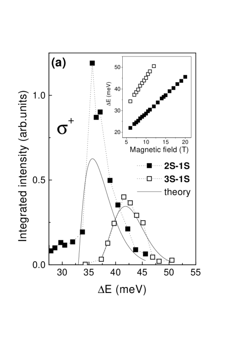
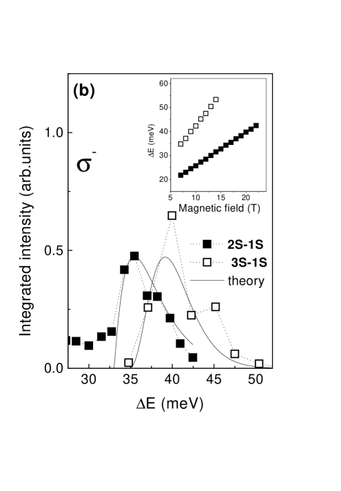
Figure 2: Integrated intensities of the 2sHH and 3sHH PLE peaks for the both polarizations (a – $\sigma^{+}$, b – $\sigma^{-}$) as a function of the peak position $\Delta E$ measured from the 1sHH peak energy. Black and open squares show the experimental data. The insets present the experimental dependences of $\Delta E(B)$ for the 2sHH and 3sHH peaks.

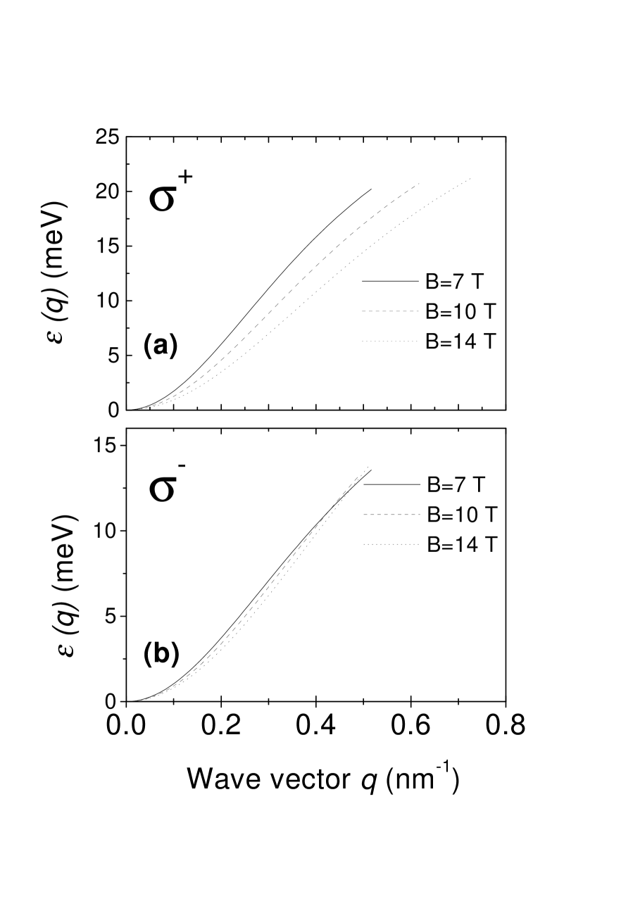
Figure 5: Transverse energy dispersion functions of Eq. (4.1) when ${\cal E}_{b}=5\,$meV; $g_{1}^{+}=0.338$, $g_{2}^{+}=0.019$, $g_{3}^{+}=0.0561$, for $\sigma^{+}$-polarization (a), and $g_{1}^{-}=-0.054$, $g_{2}^{-}=0.108$, $g_{3}^{-}=0.0459$, for $\sigma^{-}$-polarization (b).

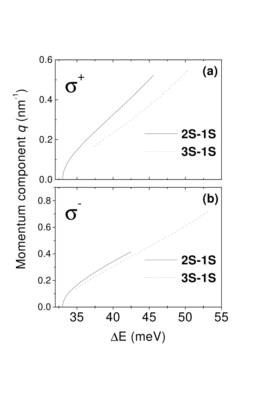
Figure 6: Values $q^{\pm}(\Delta E)$ found from the equation $\epsilon_{\pm}(q)=\Delta E-\hbar\omega_{0}$ for all transitions of $\sigma^{+}$ (a) and $\sigma^{-}$ (b) polarizations.

References

- (1) G. Bastard, Wave Mechanics Applied to Semiconductor Heterojunctions (Les éditions de physique, Les Ulis, 1988).
- (2) E. L. Ivchenko, and G. E. Pikus, Superlattices and Other Heterostructures: Symmetry a. Optical Phenomena (Springer-Verlag, Berlin, 1995).
- (3) B. Jusserand, D. Paquet, A. Regreny, Phys. Rev. B 30, 6245 (1984).
- (4) A. K. Sood, J. Menendez, M. Cardona, and K. Ploog, Phys. Rev. Lett. 54, 2111 (1985); ibid 54, 2115 (1985).
- (5) T. Tsuchiva, H. Akera, T. Ando, Phys. Rev. B 39, 6025 (1989).
- (6) J. Menéndez, J. of Lum. 44, 285 (1989).
- (7) V. F. Sapega, M. P. Chamberlain, T. Ruf, M. Cardona, D. N. Mirlin, K. Totemeyer, A. Fischer, and K. Eberl, Phys. Rev. B 52, 14144 (1995).
- (8) Yu. A. Pusep, S. W. da Silva, J. C. Galzerani, A. G. Milekhin, V. V. Preobrazhenskii, B. R. Semyagin, and I. I. Marahovka, Phys. Rev. B 52, 2610 (1995).
- (9) G. Bastard, E. E. Mendez, L. L. Chang, and L. Esaki, Phys. Rev. 26, 1974 (1982).
- (10) R. L. Greene, K. K. Bajaj, and D. E. Phelps, Phys. Rev. B 29, 1807 (1984).
- (11) L. Via , G. E. W. Bauer, M. Potemski, J. C. Maan, E. E. Mendez, and W. I. Wang, Phys. Rev. B 41, 10767 (1990).
- (12) M. Bayer, T. L. Reinecke, S. N. Walck, V. B. Timofeev, and A. Forchel, Phys. Rev. B 58, 9648 (1998).
- (13) K. Fujiwara, K. Kawashima, T. Yamamoto, N. Sano, R. Gingolani, H. T. Grahn, and K. Ploog, Phys. Rev. B 49, 1809 (1994).
- (14) V. Mizeikis, D. Birkedal, W. Langebein, V. G. Lysenko, and J. M. Hvam, Phys. Rev. B 55, 5284 (1997).
- (15) A. I. Tartakovskii, V. B. Timofeev, V. G. Lyssenko, D. Birkedal, and J. V. Hvam, JETP 85, 601 (1997).
- (16) D. N. Mirlin, I. Ja. Karlik, L. P. Nikitin, I. I. Reshina, and V. F. Sapega, Solid State Commun. 37, 757 (1981).
- (17) T. Ruf, in Phonon Raman Scattering in Semiconductors, Quantum Wells and Superlattices, Vol. 142 of Springer Tracts in Modern Physics (Springer-Verlag, Berlin, 1998) p.163.
- (18) J. A. Kash, Phys. Rev. B 47, 1221 (1993).
- (19) J. A. Kash, M. Zachau, M. A. Tischler, and U. Ekenberg, Phys. Rev. Lett. 69, 2260 (1992); M. Zachau, J. A. Kash, and W. T. Masselink, Phys. Rev. B 44, 4048 (1991).
- (20) F. Meseguer, F. Calle, C. López, J. M. Calleja, L. Via, C. Tejedor, and K. Ploog, in Proceedings of the 20th International Conference on the Physics of Semiconductors, edited by E. M. Anastassakis and J. D. Joannopoulos (World Scietific, Singapore, 1990), p. 1461.
- (21) L. P. Gor’kov and I. E. Dzyaloshinskii, Sov. Phys. JETP 26, 449 (1968).
- (22) I. V. Lerner and Yu. E. Lozovik, Sov. Phys. JETP 51, 588 (1980).
- (23) J. A. Brum and G. Bastard, J. Phys. C 18, L789 (1985).
- (24) M. M. Dignam and J. E. Sipe, Phys. Rev. B 41, 2865 (1990).
- (25) A. Chomette, B. Lambert, D. Deveaud, F. Clerot, A. Regreny, and G. Bastard, Europhys. Lett. 4, 461 (1987).
- (26) H. Chu and Y-C. Chang, Phys. Rev. B 39, 10861 (1989).
- (27) A. Chomette, B. Deveaud, F. Clérot, B. Lambert, and A. Regreny, J. of Lum. 44, 265 (1989).
- (28) D. M. Whittaker, Phys. Rev. B 41, 3238 (1990).
- (29) M. M. Dignam and J. E. Sipe, Phys. Rev. B 43, 4097 (1991).
- (30) P. Hawker, A. J. Kent, L. J. Challis, M. Henini, and O. H. Hughes, J. Phys.: Condensed Matter 1, 1153 (1989).
- (31) D. J. Barnes, R. J. Nicholas, F. M. Peeters, X-G. Wu, J. T. Devreese, J. Singleton, C. J. G. M. Langerak, J. J. Harris, and C. T. Foxon, Phys. Rev. Lett. 66, 794 (1991).
- (32) T. A. Vaughan, R. J. Nicholas, C. J. G. M. Langerak B. N. Murdin, C. R. Pidgeon, N. J. Mason, and P. J. Walker, Phys. Rev. B 53, 16481 (1996).
- (33) The energy of 1sHH which we will use in the following cannot be extracted from this set of spectra but its dependence on magnetic field was obtained from the similar experiment previously (see Ref. [14]). In particular, for this energy is meV.
- (34) For example see D. Wong, H. K. Kim, Z. Q. Fang, T. E. Schlesinger, and A. G. Milnes J. Appl. Phys. 66, 2002 (1989); C. V. Reddy, S. Fung, and C. D. Beling, Phys. Rev. B 54, 11290 (1996).
- (35) V. F. Gantmakher and Y. B. Levinson, Carrier Scattaring in Metals and Semiconductors (North-Holland, Amsterdam, 1987).
- (36) K. J. Nash and D. J. Mowbray, J. of Lum. 44, 315 (1989).
- (37) A simple estimate for the miniband width is , where the factor characterizes the wave function attenuation in the barrier which depends on the barrier height. If only is changed by factor 8/3, we arrive at the indicated estimate.