Effect of Interdots Electronic Repulsion in the Majorana Signature for a Double Dot Interferometer

Abstract

We investigate theoretically the features of the Majorana hallmark in the presence of Coulomb repulsion between two quantum dots describing a spinless double dot interferometer, where one of the dots is strongly coupled to a Kitaev wire within the topological phase. Such a system has been originally proposed without Coulomb interaction in J. of Appl. Phys. 116, 173701 (2014). Our findings reveal that for dots in resonance, the ratio between the strength of Coulomb repulsion and the dot-wire coupling changes the width of the Majorana zero-bias peak for both Fano regimes studied, indicating thus that the electronic interdots correlation influences the Majorana state lifetime in the dot hybridized with the wire. Moreover, for the off-resonance case, the swap between the energy levels of the dots also modifies the width of the Majorana peak, which does not happen for the noninteracting case. The results obtained here can guide experimentalists that pursuit a way of revealing Majorana signatures.

1 Introduction

Recently, the pursuit for Majorana quasiparticles in condensed matter systems has attracted a lot of attention, since they are one of the most promising candidate to build a quantum bit, the fundamental structure of quantum computation [1, 2]. In this sense, topological superconductors have been broadly studied, once they can host zero-energy modes of Majorana bound states (MBSs) in their edges [3-5]. The Kitaev wire within the topological phase is an example [3], since in such a proposal a 1D topological p-wave superconductor gives rise to MBSs attached to its edges. Experimentally, this setup can be implemented by putting a semiconductor nanowire, with strong spin-orbit coupling, close to an s-wave superconductor and under an external magnetic field. In this situation, p-wave topological superconductivity is induced in the nanowire by the so-called proximity effect [6-9].

The MBSs can be detected in electronic transport measurements by attaching quantum objects to them, as for instance quantum dots (QDs) [10-21]. In the case of a single QD coupled to a MBS, a zero-bias anomaly (ZBA) is theoretically predicted to appear in the conductance, with amplitude $0.5G_{0}$, where $G_{0}=e^{2}/h$ is the quantum of conductance [13]. The emergence of the ZBA is due to the leaking of the MBS zero-mode into the QD [14]. Such an anomaly was first detected experimentally by Mourik et al. [19], where the MBSs are supposed to exist once the ZBA in the conductance persists even at high gate voltages and magnetic fields. However, another physical phenomena can lead to the ZBA, as for instance the Kondo effect. Within this perspective, the detection of Majorana excitations becomes inconclusive.

Alternatives have been proposed in order to obtain the MBSs, involving ferromagnetic chains on top of s-wave superconductors with strong spin-orbit parameter [23-27]. Such a setup allows the emulation of the Kitaev wire, once the p-wave topological superconductivity is induced in the ferromagnetic atoms, yielding MBSs at the chain boundaries. Recently, this proposal has been accomplished experimentally, by using Fe atoms on a Pb superconductor surface [26]. The electronic conductance features have been measured by using an STM tip, in which the ZBA was verified at the ends of the Fe chain, thus suggesting the presence of MBSs. However, the ZBA obtained cannot be associated exclusively to the presence of MBSs [28] and, therefore the issue of Majorana detection has not been solved completely yet.

In this scenario, in order to detect MBSs new proposals become necessary. In our previous work [16], we proposed theoretically a helpful tool to detect MBSs in a system composed by a spinless double dot interferometer, with two noninteracting QDs, where one of them is coupled to one edge of the Kitaev wire within the topological phase. Such a spinless system can be achieved experimentally by applying a magnetic field strong enough to provide a Zeeman splitting in the energy levels of the QDs and metallic leads as well. Thus, just one spin orientation prevails. We found that the ZBA is robust and independent on the Fano regime of interference [29]. Additionally, we developed a novel manner to verify the presence of MBSs, which looks beyond the ZBA signature: through simulations of transmittance as a function of the detuning for the energy levels of the QDs and Fermi energy for the metallic leads, we found that a MBS has a particular way of breaking the symmetry of such transmittance profiles, which can be experimentally accessed by conductance measurements. Here we explore the same device studied in the previous work (Fig. 1), but now we consider the Coulomb repulsion between the QDs employing the Hubbard I approximation [30] in order to close the system of Green functions. Such a mean field approach is valid for $T\gg T_{K}$, where $T_{K}$ is the Kondo temperature [31]. Interestingly enough, it is possible to observe a Kondo peak even in absence of the spin degree of freedom in our double dot system, i.e, in the spinless regime. Such a specific condition is requested to ensure the topological superconductivity in the framework of the Kitaev wire. According to Ref.[31], the spinless Hamiltonian for a double dot setup can be mapped into an effective one describing a single dot, in which the spin degree of freedom is restored, thus allowing the possibility of the Kondo effect when $T\ll T_{K}.$ In this case, the pseudo localized moment of the dot is screened by those from the effective conduction band of the model via an antiferromagnetic exchange interaction, as in the standard Kondo effect. Such a phenomenon can be prevented for $T\gg T_{K},$ which is the range wherein this work focus on, thus ensuring the employment of the Hubbard I approach. Such a method is a well-established procedure in the literature that allows to catch the key features concerning the Physics away from the Kondo limit. Otherwise, the ZBA would be the outcome of a competition between the Majorana and Kondo phenomena [32].

Our findings reveal that the ZBA $0.5$ characteristic amplitude of the MBS remains even in the presence of Coulomb repulsion between the QDs, with slight fluctuations around such a value. However, for the case of QDs in resonance, the ratio between the Coulomb repulsion and the QD-wire coupling modifies the ZBA width, revealing thus that the electronic interdots repulsion affects the Majorana state lifetime in the QD. Moreover, in the interacting system the width of the Majorana signature also is influenced by swapping the energy levels of the QDs, which does not occur without Coulomb repulsion.

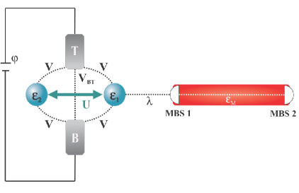
Figure 1: (Color online) Sketch of the system proposed: a Kitaev wire hosting Majorana bound states (MBSs) in its edges (white half-spheres) side-coupled to a spinless double dot interferometer. This device is composed by metallic leads (Bottom(B) and Top(T)) and two quantum dots, with energy levels $\varepsilon_{1}$ and $\varepsilon_{2}$, respectively. $U$ represents the intensity of the interdots Coulomb repulsion, $V$ is the tunneling amplitude between the QDs and leads. The coupling lead-lead is given by $V_{BT}.$ The wire is coupled to the QD 1 by the strength $\lambda.$ The overlap between the wave functions of the MBS 1 and MBS 2 is denoted by $\varepsilon_{M}$ and $\varphi$ is the bias-voltage of the setup.

2 Theoretical Model

To describe the system presented in Fig. 1 we use the Hamiltonian inspired on the original proposal from Liu and Baranger [13],

$$\mathcal{H} =\sum_{\alpha k}\tilde{\varepsilon}_{\alpha k}c_{\alpha k}^{\dagger}c_{\alpha k}+\sum_{j}\varepsilon_{j}d_{j}^{\dagger}d_{j}+Ud_{1}^{\dagger}d_{1}d_{2}^{\dagger}d_{2}$$

$$+\mathcal{H}_{\text{{lead-dot}}}+\mathcal{H}_{\text{{lead-lead}}}+\mathcal{H}_{\text{{MBSs}}},$$ (1)

where the operator $c_{\alpha k}^{\dagger}$ ($c_{\alpha k}$) creates (annihilates) an electron in the lead $\alpha$= B/T (Bottom/Top), with energy $\tilde{\varepsilon}_{\alpha k}=\varepsilon_{k}-\mu_{\alpha}$, wherein $\mu_{\alpha}$ as the chemical potential and $k$ is the wave number. We consider $\mu_{B}-\mu_{T}=2\Delta\mu=e\varphi$ as the bias between the leads, where $e>0$ is the electron charge and $\varphi$ is the bias-voltage. $d_{j}^{\dagger}$ ($d_{j}$) creates (annihilates) an electron in the state $\varepsilon_{j}$ in the QDs and $U$ is the interdots Coulomb repulsion, with $j=1,2.$ $\mathcal{H}_{\text{{lead-dot}}}=V\sum_{\alpha kj}(c_{\alpha k}^{\dagger}d_{j}+\text{{H.c.}}),$ where $V$ is the coupling amplitude between the leads and the QDs, and $\mathcal{H}_{\text{{lead-lead}}}=V_{BT}\sum_{kp}(c_{Bk}^{\dagger}c_{Tp}+\text{{H.c.}})$, with $V_{BT}$ the direct lead-lead hybridization. Furthermore,

$$\mathcal{H}_{\text{{MBSs}}}=i\varepsilon_{M}\Psi_{1}\Psi_{2}+\lambda(d_{1}-d_{1}^{\dagger})\Psi_{1}$$ (2)

describes an effective model for the Kitaev wire within the topological phase, where $\Psi_{l}=\Psi_{l}^{\dagger}$ is the Majorana operator, with $l=1,2.$ The MBS 1 $\Psi_{1}$ and MBS 2 $\Psi_{2}$ are connected via $\varepsilon_{M}\sim e^{-L/\xi}$, where $L$ is the distance between them and $\xi$ is the superconductor coherence length. The coupling strength between the MBS 1 and QD 1 is $\lambda.$ According to the Landauer-Büttiker formula [33] for the zero-bias regime, the conductance depends on the transmittance $\mathcal{T}(\varepsilon)$ as follows:

$$G=G_{0}\int d\varepsilon\left(-\frac{\partial f_{F}}{\partial\varepsilon}\right)\mathcal{T}(\varepsilon),$$ (3)

where $f_{F}$ is the Fermi-Dirac distribution.

In order to obtain the transmittance, within the wide band limit, we perform the transformations $c_{Bk}=\frac{1}{\sqrt{2}}(c_{ek}+c_{ok})$ and $c_{Tk}=\frac{1}{\sqrt{2}}(c_{ek}-c_{ok})$ in the Hamiltonian of Eq. (1), which depends on the even and odd conduction operators $c_{ek}$ and $c_{ok}$, respectively. Thus, Eq. (1) becomes $\mathcal{H}=\mathcal{H}_{e}+\mathcal{H}_{o}+\mathcal{\tilde{H}}_{\text{{tun}}}=\mathcal{H}_{\varphi=0}+\mathcal{\tilde{H}}_{\text{{tun}}},$ where

$$\mathcal{H}_{e}=\sum_{k}\varepsilon_{k}c_{ek}^{\dagger}c_{ek}+\sum_{j}\varepsilon_{j}d_{j}^{\dagger}d_{j}+ Ud_{1}^{\dagger}d_{1}d_{2}^{\dagger}d_{2}$$

$$+\sqrt{2}V\sum_{jk}(c_{ek}^{\dagger}d_{j}+\text{{H.c.}})+V_{BT}\sum_{kp}c_{ek}^{\dagger}c_{ep} +\mathcal{H}_{\text{{MBSs}}}$$

describes effectively the couplings between leads and QDs via the strength $\sqrt{2}V$ and $\mathcal{H}_{o}=\sum_{k}\varepsilon_{k}c_{ok}^{\dagger}c_{ok}-V_{BT}\sum_{kp}c_{ok}^{\dagger}c_{op}$ is for the part of the system decoupled from the QDs. $\mathcal{H}_{e}$ is connected to $\mathcal{H}_{o}$ by the tunneling Hamiltonian $\mathcal{\tilde{H}}_{\text{{tun}}}=-\Delta\mu\sum_{k}(c_{ek}^{\dagger}c_{ok}+c_{ok}^{\dagger}c_{ek}),$ which in the zero-bias regime is perturbative, since $\Delta\mu\rightarrow 0$ due $\varphi\rightarrow 0.$ Thus, according to the linear response theory and by applying the equation of motion method (EOM) [33], the transmittance [16] is given by

$$\frac{\mathcal{T}\left(\varepsilon\right)}{\mathcal{T}_{b}} =1+(1-q_{b}^{2})\tilde{\Gamma}\sum_{j\tilde{j}}\text{{Im}}(\tilde{\mathcal{G}}_{d_{j},d_{\tilde{j}}})$$

$$+2q_{b}\tilde{\Gamma}\sum_{j\tilde{j}}\text{{Re}}(\tilde{\mathcal{G}}_{d_{j},d_{\tilde{j}}}),$$ (5)

where $\mathcal{T}_{b}=\frac{4x}{\left(1+x\right)^{2}}$ represents the background transmittance with $x=(\pi\rho_{0}V_{BT})^{2}$, $\rho_{0}$ is the leads density of states, $\tilde{\Gamma}=\frac{\Gamma}{1+x}$ is an effective QD-leads coupling, with $\Gamma=2V^{2}\pi\rho_{0}$, and $q_{b}=\sqrt{\frac{\mathcal{R}_{b}}{\mathcal{T}_{b}}}=\frac{\left(1-x\right)}{2\sqrt{x}}$ is the Fano parameter [29, 34], where $\mathcal{R}_{b}$ represents the corresponding background reflectance.

With the aim to get the retarded Green functions of the system, we first express the Majorana operators $\Psi_{1}$ and $\Psi_{2}$ in terms of a nonlocal regular fermion state $f$, according to the following relations: $\Psi_{1}=\frac{1}{\sqrt{2}}(f^{\dagger}+f)$ and $\Psi_{2}=i\frac{1}{\sqrt{2}}(f^{\dagger}-f),$ with $f\neq f^{\dagger}$ and $[f,f^{\dagger}]_{+}=1.$ Then, Eq. (2) becomes $\mathcal{H}_{\text{{MBSs}}}=\varepsilon_{M}(f^{\dagger}f-\frac{1}{2})+\frac{\lambda}{\sqrt{2}}(d_{1}f^{\dagger}+fd_{1}^{\dagger})+\frac{\lambda}{\sqrt{2}}(d_{1}f-d_{1}^{\dagger}f^{\dagger}).$

The EOM procedure [33] can be summarized as

$$(\varepsilon+i0^{+})\tilde{\mathcal{G}}_{\mathcal{AB}}=[\mathcal{A},\mathcal{B^{\dagger}}]_{+}+\tilde{\mathcal{G}}_{\left[\mathcal{A},\mathcal{\mathcal{H}}_{i}\right]\mathcal{B}}$$ (6)

where $\tilde{\mathcal{G}}_{\mathcal{AB}}$ represents the retarded Green function in the energy domain $\varepsilon$, with $\mathcal{A}$ and $\mathcal{B}$ as fermionic operators belonging to the Hamiltonian $\mathcal{\mathcal{H}}_{i}$. The Green function for the QD in the time domain $t$ is definite by

$$\mathcal{G}_{d_{j}d_{l}}(t)=-\frac{i}{\hbar}\theta\left(t\right){\tt Tr}\{\varrho_{\text{{e}}}[d_{j}\left(t\right),d_{l}^{\dagger}\left(0\right)]_{+}\},$$ (7)

wherein $\theta\left(t\right)$ is the Heaviside step function and $\varrho_{\text{e}}$ is the density-matrix for Eq. (LABEL:eq:even). By applying the EOM procedure in Eq. (7), we obtain

$$(\varepsilon-\varepsilon_{j}-\Sigma-\delta_{j1}\Sigma_{\text{{MBS1}}})\tilde{\mathcal{G}}_{d_{j}d_{l}}=\delta_{jl}+ \Sigma[\underset{\tilde{l}\neq j}{\sum}\tilde{\mathcal{G}}_{d_{j}d_{\tilde{l}}}]$$

$$+U[\tilde{\mathcal{G}}_{d_{j}n_{\bar{j}},d_{l}}+\lambda^{2}\tilde{K}\delta_{j1}\tilde{\mathcal{G}}_{d_{j}^{\dagger}n_{\bar{j}},d_{l}}]$$ (8)

where the index $\bar{j}$ represents the opposite of $j$, i.e, $j\leftrightarrow\bar{j}\equiv 1\leftrightarrow 2$, with $\Sigma=-\frac{(\sqrt{x}+i)}{1+x}\Gamma$ and $\Sigma_{\text{{MBS1}}}=\lambda^{2}K(1+\lambda^{2}\tilde{K})$ as the self-energies that appear in the noninteracting case [16], where $K=\frac{1}{2}\left(\frac{1}{\varepsilon-\varepsilon_{M}+i0^{+}}+\frac{1}{\varepsilon+\varepsilon_{M}+i0^{+}}\right)$, $\tilde{K}=\frac{K}{\varepsilon+\varepsilon_{1}+\tilde{\Sigma}-\lambda^{2}K}$ and $\tilde{\Sigma}$ is the complex conjugate of $\Sigma.$ We point out that making $U=0$ in Eq. (8), we obtain the same expression of the noninteracting system [Eq.(17) of Ref. [16]]. By applying the EOM approach in the same way we have performed above, we obtain the retarded Green functions of four operators $\tilde{\mathcal{G}}_{d_{j}n_{\bar{j}},d_{l}}$ and $\tilde{\mathcal{G}}_{d_{j}^{\dagger}n_{\bar{j}},d_{l}}$, given by

$$(\varepsilon-\varepsilon_{j}-U+i0^{+})\tilde{\mathcal{G}}_{d_{j}n_{\bar{j}},d_{l}} =\delta_{jl}\bigl{\langle}n_{\bar{j}}\bigr{\rangle}$$

$$+\sqrt{2}V\sum_{k}[\tilde{\mathcal{G}}_{n_{\bar{j}}c_{ek},d_{l}}+\tilde{\mathcal{G}}_{d_{\bar{j}}^{\dagger}c_{ek}d_{j},d_{l}} -\tilde{\mathcal{G}}_{c_{ek}^{\dagger}d_{\bar{j}}d_{j},d_{l}}]$$

$$+\frac{\lambda}{\sqrt{2}}[\delta_{\bar{j}1}\tilde{\mathcal{G}}_{f^{\dagger}d_{\bar{j}}d_{j},d_{l}}-\delta_{\bar{j}1}\tilde{\mathcal{G}}_{d_{\bar{j}}^{\dagger}fd_{j},d_{l}} -\delta_{j1}\tilde{\mathcal{G}}_{n_{\bar{j}}f,d_{l}}]$$

$$+\frac{\lambda}{\sqrt{2}}[\delta_{\bar{j}1}\tilde{\mathcal{G}}_{\eta d_{\bar{j}}d_{j},d_{l}}-\delta_{\bar{j}1}\tilde{\mathcal{G}}_{d_{\bar{j}}^{\dagger}\eta^{\dagger}d_{j},d_{l}} -\delta_{j1}\tilde{\mathcal{G}}_{n_{\bar{j}}\eta^{\dagger},d_{l}}]$$

and

$$(\varepsilon+\varepsilon_{j}+U+i0^{+})\tilde{\mathcal{G}}_{d_{j}^{\dagger}n_{\bar{j}},d_{l}}= \delta_{\bar{j}l}\bigl{\langle}d_{j}^{\dagger}d_{\bar{j}}^{\dagger}\bigr{\rangle}$$

$$+\sqrt{2}V\sum_{k}[\tilde{\mathcal{G}}_{d_{\bar{j}}^{\dagger}c_{ek}d_{j}^{\dagger},d_{l}}-\tilde{\mathcal{G}}_{c_{ek}^{\dagger}d_{\bar{j}}d_{j}^{\dagger},d_{l}} -\tilde{\mathcal{G}}_{n_{\bar{j}}c_{ek}^{\dagger},d_{l}}]$$

$$+\frac{\lambda}{\sqrt{2}}[\delta_{j1}\tilde{\mathcal{G}}_{n_{\bar{j}}f^{\dagger},d_{l}}-\delta_{\bar{j}1}\tilde{\mathcal{G}}_{d_{\bar{j}}f^{\dagger}d_{j}^{\dagger},d_{l}}+ \delta_{\bar{j}1}\tilde{\mathcal{G}}_{fd_{\bar{j}}^{\dagger}d_{j}^{\dagger},d_{l}}]$$

$$+\frac{\lambda}{\sqrt{2}}[\delta_{j1}\tilde{\mathcal{G}}_{n_{\bar{j}}f,d_{l}}-\delta_{\bar{j}1}\tilde{\mathcal{G}}_{d_{\bar{j}}fd_{j}^{\dagger},d_{l}}+ \delta_{\bar{j}1}\tilde{\mathcal{G}}_{f^{\dagger}d_{\bar{j}}^{\dagger}d_{j}^{\dagger},d_{l}}].$$

with expectation values

$$\bigl{\langle}n_{\bar{j}}\bigr{\rangle}=\bigl{\langle}d_{\bar{j}}^{\dagger}d_{\bar{j}}\bigr{\rangle}=(-\frac{1}{\pi})\int_{-\infty}^{\infty}\text{{d$\varepsilon$}}f_{F}(\varepsilon)\text{{Im}}\{\tilde{\mathcal{G}}_{d_{\bar{j}}d_{\bar{j}}}\}$$ (11)

and

$$\bigl{\langle}d_{j}^{\dagger}d_{\bar{j}}^{\dagger}\bigr{\rangle}=(-\frac{1}{\pi})\int_{-\infty}^{\infty}\text{{d$\varepsilon$}}f_{F}(\varepsilon)\text{{Im}}\{\tilde{\mathcal{G}}_{d_{j}^{\dagger}d_{\bar{j}}}\}.$$ (12)

As one can see in Eqs. (11) and (12), a self-consistent calculation is required to obtain the electronic occupation number for the QDs $\bigl{\langle}n_{\bar{j}}\bigr{\rangle}=\bigl{\langle}d_{\bar{j}}^{\dagger}d_{\bar{j}}\bigr{\rangle}$ and the expectation value of the delocalized Cooper paring $\bigl{\langle}d_{j}^{\dagger}d_{\bar{j}}^{\dagger}\bigr{\rangle}$. As the latter amount is induced in the QDs due to the presence of the Kitaev wire, such a quantity is expected to be smaller compared to the usual occupation number [32]. We have confirmed this feature in the self-consistent process.

In order to close the system of Green functions, we apply an approximation method motivated by the Hubbard I decoupling [30], which can be summarized as $\tilde{\mathcal{G}}_{\mathcal{ABCD}}=\left\langle\mathcal{AB}\right\rangle\tilde{\mathcal{G}}_{\mathcal{CD}}$, with the property $\left\langle\mathcal{AB}\right\rangle=\left\langle\mathcal{B}^{\dagger}\mathcal{A}^{\dagger}\right\rangle$. After this procedure, we obtain:

$$(\varepsilon-\varepsilon_{j}-\Sigma^{(j)}-\delta_{j1}\Sigma_{\text{{MBS1}}}^{\text{{full}}})\tilde{\mathcal{G}}_{d_{j}d_{j}}= 1$$

$$+\frac{U\bigl{\langle}n_{\bar{j}}\bigr{\rangle}}{(\varepsilon-\varepsilon_{j}-U+i0^{+})}+\Sigma^{(j)}\tilde{\mathcal{G}}_{d_{j}d_{\bar{j}}}$$ (13)

and

$$(\varepsilon-\varepsilon_{j}-\Sigma^{(j)}-\delta_{j1}\Sigma_{\text{{MBS1}}}^{\text{{full}}})\tilde{\mathcal{G}}_{d_{j}d_{\bar{j}}}=$$

$$\delta_{j1}U\lambda^{2}\tilde{K}_{U}\bigl{\langle}d_{j}^{\dagger}d_{\bar{j}}^{\dagger}\bigr{\rangle}(\frac{U\bigl{\langle}n_{\bar{j}}\bigr{\rangle}}{\varepsilon-\varepsilon_{j}-U+i0^{+}}+1)$$

$$+\Sigma^{(j)}\tilde{\mathcal{G}}_{d_{\bar{j}}d_{\bar{j}}},$$ (14)

where $\tilde{K}_{U}=\frac{\tilde{K}}{(\varepsilon+\varepsilon_{j}+U-\sigma+\delta_{j1}\bigl{\langle}n_{\bar{j}}\bigr{\rangle}U\lambda^{2}\tilde{K})}$ and $\sigma=\frac{\tilde{\Sigma}\bigl{\langle}n_{\bar{j}}\bigr{\rangle}U}{\varepsilon+\varepsilon_{j}+\tilde{\Sigma}-\delta_{j1}\lambda^{2}K}$. Notice that we find

$$\Sigma^{(j)}=\Sigma(1+\frac{U\bigl{\langle}n_{\bar{j}}\bigr{\rangle}}{\varepsilon-\varepsilon_{j}-U+i0^{+}})$$ (15)

and

$$\Sigma_{\text{{MBS1}}}^{\text{{full}}}=\Sigma_{\text{{MBS1}}}+\frac{U\bigl{\langle}n_{2}\bigr{\rangle}\Sigma_{\text{{MBS1}}}}{(\varepsilon-\varepsilon_{1}-U+i0^{+})}$$

$$-U\bigl{\langle}n_{2}\bigr{\rangle}\lambda^{2}\tilde{K}_{U}(\frac{U\bigl{\langle}n_{2}\bigr{\rangle}}{\varepsilon-\varepsilon_{1}-U+i0^{+}}+1)\times$$

$$(\Sigma_{\text{{MBS1}}}-\tilde{\Sigma}\lambda^{2}\tilde{K})$$ (16)

as the self-energies dressed by the interdots Coulomb repulsion. We highlight that these expressions recover the well know results for the noninteracting case $U=0$, as we found in Ref. [16].

3 Results and Discussion

In what follows we discuss the effect of the Coulomb interdots correlation in the Majorana signature. The entire analysis performed here is for the case of a long wire, in such a way that the overlap between the wave functions of the MBSs can be neglected $(\varepsilon_{M}=0)$. Additionally, we adopt in our simulations the model parameters of the system Hamiltonian, in units of $\Gamma=2V^{2}\pi\rho_{0}$. The transmittance profiles [Eq. (5)] as a function of the Fermi energy for metallic leads are presented in Fig. 2, in particular for the case of QDs in resonance $(\varepsilon_{1}=\varepsilon_{2}=-8\Gamma)$. The left panels [Figs. 2(a), (b) and (c)] are for the Fano regime $q_{b}\rightarrow\infty$ $(x=0),$ where the electronic path is completely through the QDs, while the right panels [Figs. 2(d), (e) and (f)] show the opposite case, where the electrons travel preferentially via leads ($q_{b}=0$, $x=1$). In Fig. 2(a), the Kitaev wire is decoupled from the noninteracting QDs $(U=0$, $\lambda=0)$, and leads to a resonance pinned at the energy levels of these QDs. For the interacting case $(U=16\Gamma)$ [Fig. 2(b)], but still without wire, the transmittance profile displays the Hubbard bands, represented by two peaks pinned at $\varepsilon_{j}$ and $\varepsilon_{j}+U$, respectively, where we consider the particle-hole symmetric point $(2\varepsilon_{j}+U=0)$ of the system Hamiltonian. Fig. 2(c) displays the case where the wire is strongly coupled to interferometer with interacting QDs $(\lambda=80\Gamma$ and $U=16\Gamma)$. As one can see, a zero-bias peak with 0.5 amplitude emerges making explicit that the MBS 1 at the wire edge leaked into the QD 1. Such a panel also exhibits two peaks fixed at $\varepsilon_{j}$ and $\varepsilon_{j}+U$ as in the upper case, but slightly narrower, which is an effect due to the presence of the wire. The opposite Fano regime (right panels) presents the same behavior showed in Figs. 2(a), (b) and (c), but the peaks are replaced by dips, in agreement with the standard Fano theory of interference [29].

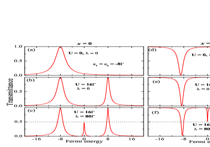
Figure 2: (Color online) Transmittance of Eq. (5) as a function of the leads Fermi energy for two distinct Fano regimes. The left panels [(a), (b) and (c)] show the case wherein the electronic tunneling occurs via QDs $(x=0$, $q_{b}\rightarrow\infty),$while the right panels [(d), (e) and (f)] exhibit the opposite Fano regime, where the electronic path is preferentially through the metallic leads $(x=1$, $q_{b}=0).$

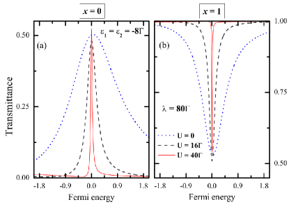
Figure 3: (Color online) Transmittance profiles of Eq. (5) as a function of leads Fermi energy display the effect of Coulomb interaction in the Majorana hallmark for distinct Fano regimes: (a)$x=0$, $q_{b}\rightarrow\infty$ and (b)$x=1$, $q_{b}=0$.

In Fig. 3 we analyze the effect of the Coulomb repulsion in the Majorana signature, namely the ZBA, for both Fano regimes. The QDs are still in resonance and the wire is strongly coupled to QD 1. The dotted-blue line shows the noninteracting case $(U=0)$, where we can verify a ZBA characterized by a broad width in the two Fano cases $(x=0$ and $x=1)$. Notice that there is a small difference between the amplitudes: for the case where $x=0$ [Fig. 3(a)] the amplitude is exactly 0.5, while in $x=1$ [Fig. 3(b)] it is $<0.5$. Such a feature is due to the presence of the QD 2 and a more detailed discussion can be found in Ref. [15]. As we increase the Coulomb interaction (dashed-black line for $U=16\Gamma$ and red line for $U=40\Gamma$), the ZBA becomes narrower and shows a slight fluctuation around the 0.5 amplitude, verified in both Fano regimes. This change in the ZBA width suggests that the Majorana state lifetime within the QD 1 increases due to the electronic correlation effects between the QDs, since this lifetime is inversely proportional to such a width [35].

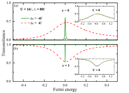
Figure 4: (Color online) Transmittance of Eq. (5) as a function of leads Fermi energy, in the situation where the energy levels of QDs are off-resonance, leading to a finite detuning $\Delta\varepsilon=\varepsilon_{2}-\varepsilon_{1}.$ The green line represents the case where $\varepsilon_{1}=-4\Gamma$ and $\varepsilon_{2}=-8\Gamma$, while the dashed-red line depicts for $\varepsilon_{1}=-8\Gamma$ and $\varepsilon_{2}=-4\Gamma$. The panels (a) and (b) represents the Fano regime $x=0$ $(q_{b}\rightarrow\infty)$ and $x=1$ $(q_{b}=0)$, where the corresponding insets describe the noninteracting scenario.

Fig. 4 shows transmittance profiles [Eq. (5)] as a function of leads Fermi energy for the interacting case, in the situation where the energy levels of the QDs are off-resonance, leading to a finite detuning $\Delta\varepsilon=\varepsilon_{2}-\varepsilon_{1}.$ The upper panel [Fig. 4(a)] shows the behavior of the transmittance for the Fano regime $x=0$. The Majorana peak is narrow and has an amplitude slightly higher than 0.5 when $\varepsilon_{1}=-4\Gamma$ and $\varepsilon_{2}=-8\Gamma$ (green line). By making a swap in the energy levels of the QDs, i.e. $\varepsilon_{1}=-8\Gamma$ and $\varepsilon_{2}=-4\Gamma,$ the width of the Majorana peak increases significantly and exhibits a 0.5 amplitude (dashed-red line). A similar behavior is observed for the opposite Fano regime [Fig. 4(b)], but as in Figs. 2 and 3, the peaks are replaced by dips. Such fluctuations observed in the width and amplitude for the ZBA arising from the MBS do not occur for the noninteracting case, as can be seen in the insets of both panels. Thus, the tuning of the energy levels for the QDs also plays an important role in the Majorana state lifetime. This particular behavior suggests that experimentally, the Majorana signature depends on the relative positions of the energy levels for the QDs.

4 Conclusions

We have studied theoretically the effects of the Coulomb repulsion in the Majorana signature in a system composed of a spinless double dot interferometer with two interacting QDs, where one of them is strongly coupled to the MBS hosted at one edge of a Kitaev wire within the topological phase. We have found that the ZBA in the transmittance, due to the MBS, appears even in the presence of interdots Coulomb interaction. For QDs in resonance, the width of this Majorana hallmark decreases as we increase the ratio between the strength of the Coulomb repulsion and the dot-wire coupling $(U/\lambda)$, together with a slight fluctuation around the $0.5$ amplitude. This narrowing of the Majorana signature also occurs when a swap between the energy levels for the QDs is performed. Such a narrowing is not verified in the noninteracting case. These features then point out that the ratio $U/\lambda$ and the relative position of the energy levels (detuning) for the QDs, constitute the key ingredients ruling the Majorana state lifetime in the QD next to the Kitaev wire. Our findings shed new light into the ZBA of MBSs in the presence of Coulomb correlations and can be helpful in the quest for Majorana signatures in condensed matter systems.

References

- [1] J. Alicea, Rep. Prog. Phys. 75, 076501 (2012).
- [2] S. R. Elliott and M. Franz, Rev. Mod. Phys. 87, 137 (2015).
- [3] A. Y. Kitaev, Phys.-Usp. 44, 131 (2001).
- [4] R. M. Lutchyn, J. D. Sau, and S. Das Sarma, Phys. Rev. Lett. 105, 077001 (2010).
- [5] Y. Oreg, G. Refael, and F. von Oppen, Phys. Rev. Lett. 105, 177002 (2010).
- [6] A. A. Zyuzin, D. Rainis, J. Klinovaja, and D. Loss, Phys. Rev. Lett. 111, 056802 (2013).
- [7] D. Rainis, J. Klinovaja, L. Trifunovic, and D. Loss, Phys. Rev. B 87, 024515 (2013).
- [8] A. Zazunov, P. Sodano, and R. Egger, New J. Phys 15, 035033 (2013).
- [9] D. Roy, C. J. Bolech, and N. Shah, Phys. Rev. B 86, 094503 (2012).
- [10] Y. Cao, P. Wang, G. Xiong, M. Gong, and X.-Q. Li, Phys. Rev. B 86, 115311 (2012).
- [11] Y.-X. Li and Z. M. Bai, J. Appl. Phys. 114, 033703 (2013).
- [12] N. Wang, S. Lv, and Y. Li, J. Appl. Phys. 115, 083706 (2014).
- [13] D. E. Liu and H. U. Baranger, Phys. Rev. B 84, 201308(R) (2011).
- [14] E. Vernek, P. H. Penteado, A. C. Seridonio, and J. C. Egues, Phys. Rev. B 89, 165314 (2014).
- [15] A. C. Seridonio, E. C. Siqueira, F. A. Dessotti, R. S. Machado, and M. Yoshida, J. Appl. Phys. 115, 063706 (2014).
- [16] F.A. Dessotti, L.S. Ricco, M.de Souza, F.M. Souza, and A.C. Seridonio, J. of Appl. Phys.116, 173701 (2014).
- [17] A. Ueda and T. Yokoyama, Phys. Rev. B 90, 081405(R) (2014).
- [18] C.-H. Lin, J. D. Sau, and S. Das Sarma, Phys. Rev. B 86, 224511 (2012).
- [19] V. Mourik, K. Zuo, S. M. Frolov, S. R. Plissard, E. P. A. M. Bakkers, and L. P. Kouwenhoven, Science 336, 1003 (2012).
- [20] A. Das, Y. Ronen, Y. Most, Y. Oreg, M. Heiblum, and H. Shtrikman, Nat. Phys. 8, 887 (2012).
- [21] E. J. H. Lee, X. Jiang, M. Houzet, R. Aguado, C. M. Lieber, and S. De Franceschi, Nat. Nanotechnol. 9, 79 (2014).
- [22] E. J. H. Lee, X. Jiang, R. Aguado, G. Katsaros, C. M. Lieber, and S. De Franceschi, Phys. Rev. Lett. 109, 186802 (2012).
- [23] S. N.-Perge, I. K. Drozdov, B. A. Bernevig, and Ali Yazdani, Phys. Rev. B 88, 020407(R) (2013).
- [24] A. Heimes, P. Kotetes, and G. Schön, Phys. Rev. B 90, 060507(R) (2014).
- [25] J. Li, H. Chen, I.K. Drozdov, A. Yazdani, B.A. Bernevig, and A.H. MacDonald, Phys. Rev. B 90, 235433 (2014).
- [26] S.N.-Perge, I.K. Drozdov, J. Li, H. Chen, S. Jeon, J. Seo, A.H. MacDonald, B.A. Bernevig, and A. Yazdani, Science 346, 602 (2014).
- [27] Y. Peng, F. Pientka, L.I. Glazman, and F. von Oppen, Phys. Rev. Lett. 114 106801 (2015).
- [28] E. Dumitrescu, B. Roberts, S. Tewari, J. D. Sau, and S. Das Sarma, Phys. Rev. B 91, 094505 (2015).
- [29] U. Fano, Phys. Rev. 124, 1866 (1961).
- [30] J. Hubbard, Proc. R. Soc. London A 276, 238 (1963).
- [31] Q.-f. Sun and H. Guo, Phys. Rev. B 66, 155308 (2002).
- [32] D. A. Ruiz-Tijerina, E. Vernek, L. G. G. V. Dias da Silva and J. C. Egues, Phys. Rev. B, 91, 115435 (2015).
- [33] H. Haug and A.P. Jauho, Quantum Kinetics in Transport and Optics of Semiconductors, Springer Series in Solid-State Sciences 123 (Springer, New York, 1996).
- [34] W. Hofstetter, J. König, and H. Schoeller, Phys. Rev. Lett. 87, 156803 (2001).
- [35] P. Phillips, Advanced Solid State Physics, 2nd Edition (Cambridge University Press, 2012).