Efficient Photo-heating Algorithms in Time-dependent Photo-ionization Simulations

Abstract

We present an extension to the time-dependent photo-ionization code C²-Ray to calculate photo-heating in an efficient and accurate way. In C²-Ray, the thermal calculation demands relatively small time-steps for accurate results. We describe two novel methods to reduce the computational cost associated with small time-steps, namely, an adaptive time-step algorithm and an asynchronous evolution approach. The adaptive time-step algorithm determines an optimal time-step for the next computational step. It uses a fast ray-tracing scheme to quickly locate the relevant cells for this determination and only use these cells for the calculation of the time-step. Asynchronous evolution allows different cells to evolve with different time-steps. The asynchronized clocks of the cells are synchronized at the times where outputs are produced. By only evolving cells which may require short time-steps with these short time-steps instead of imposing them to the whole grid, the computational cost of the calculation can be substantially reduced. We show that our methods work well for several cosmologically relevant test problems and validate our results by comparing to the results of another time-dependent photo-ionization code.

1 Introduction

Photo-ionization is a process of fundamental importance in astrophysics as it is one of the most efficient ways to convert radiation energy into thermal energy of a gas. In the photo-ionization process the excess energy of the ionizing photons is transferred to the liberated electrons which through collisions can then increase the temperature of the gas. The main sources of ionizing photons in the Universe are either young, massive stars or accretion disks around compact objects. This transfer of energy thus often constitutes a feedback process in which the formation of sources of ionizing photons change their environment. For example in star formation regions the photo-ionization of the parent molecular cloud can regulate further star formation in that region. On cosmological scales, the reionization of intergalactic medium (IGM) by radiation from stars in the first generations of galaxies can likewise be considered to be a radiative feedback process.

The temperature acquired by the photo-ionized gas depends on the one hand on the energy distribution of ionizing photons from the source and on the other hand on the effects of radiative cooling. The ionization and the increase in temperature trigger radiative cooling processes (often dominated by collisional excitation cooling) so that within a cooling time, the temperature of the gas will achieve an equilibrium value set by the balance of the photo-ionization heating rate (henceforth photo-heating rate) and the cooling rate. In typical interstellar medium (ISM) conditions, the cooling time is short compared to the growth of an ionized region and the temperature inside the HII region is close to this equilibrium value. For this reason photo-ionization codes historically focused on solving for the equilibrium case, as for example the well-known Cloudy code (Ferland et al., 2013).

However, for the low density and low, or even zero, metallicity conditions found in the IGM during cosmic reionization, the cooling time can greatly exceed the time in which the ionized region doubles its size and the temperature structure will reflect the initial photo-heating efficiency, thus carrying important information about the source properties and gas density (Theuns et al., 2002; Hui & Haiman, 2003; Cen et al., 2009). In this case, the calculation of the time-dependent photo-heating should be performed carefully to achieve a correct answer.

The impact of photo-heating onto the IGM temperature during cosmic reionization can be probed by two methods, either by analysis of IGM absorption lines in quasar spectra, at the highest redshifts dominated by Lyman-$\alpha$ absorption, or by observations of the redshifted 21cm signal from HI.

Quasar spectra display absorption blueward of the Lyman-$\alpha$ (Ly$\alpha$) line center due to the presence of HI in the IGM. The line width (or Doppler width) of these absorption features can be used to measure the temperature of the IGM. Close to the end of reionization the mean density of neutral hydrogen in the IGM is high enough to scatter all of the Ly$\alpha$ radiation out of the line-of-sight (the so-called Gunn-Peterson trough). However, through their high luminosity quasars are capable of creating more highly ionized regions of typical sizes $\sim 10$ proper Mpc around themselves, the so-called quasar near zone, in which it is possible to identify Ly$\alpha$ absorption lines. From the properties of these lines constraints on the IGM ionization state and quasar properties can be derived (Fan et al., 2006; Bolton & Haehnelt, 2007; Willott et al., 2007; Mesinger & Haiman, 2007; Bolton et al., 2011; Schroeder et al., 2013), as well as constraints on the IGM temperature in these regions (Bolton & Haehnelt, 2007; Bolton et al., 2010, 2012). The values of these temperatures can then be used to put constraints on the redshift when the reionization was complete (Raskutti et al., 2012).

The 21cm line is a weak, low energy transition of neutral hydrogen, which during the epoch of reionization is expected to produce an observable signal below frequencies of $\sim 200$ MHz (Furlanetto et al., 2006). The detection of signal is the major goal of a range of new low frequency radio telescopes: GMRT (Paciga et al., 2013), LOFAR (van Haarlem et al., 2013), MWA (Tingay et al., 2013), PAPER (Parsons et al., 2010) and 21CMA. This signal maps out the distribution of neutral hydrogen on the largest scales in the IGM and its detection will reveal the progress of reionization in great detail. The intensity of the signal is measured against the cosmic microwave background signal and described by the differential brightness temperature which depends on the neutral hydrogen density and the excitation or spin temperature, $T_{\mathrm{s}}$, of the neutral gas (Furlanetto et al., 2006). For most of the epoch of reionization the spin temperature is expected to be close to the kinetic temperature of the gas. An early generation of x-ray sources can mildly heat the gas through low level photo-ionization and thus leave an imprint of their presence (see e.g. Pritchard & Furlanetto, 2007).

Therefore, understanding cosmic reionization not only requires following the photo-ionization of the neutral hydrogen but also the photo-heating of the gas. Modelling this process is best accomplished with cosmological reionization simulations which follow both the evolution of the dark matter and baryonic density distribution and the transfer of ionizing photons emanating from the developing (proto-)galaxies (for a review see Trac & Gnedin, 2011).

In such simulations, the radiative transfer part, in principle requiring three spatial coordinates, two angles and a range of frequencies, dominates the total computational cost. Therefore it is important to develop and use efficient numerical methods for including radiative transfer in cosmological simulations. Over the past 15 years a range of time-dependent, three dimensional photo-ionization methods for use in cosmological simulations have been developed. Many of these have been benchmarked against each other in Iliev et al. (2006a) and Iliev et al. (2009). As can be seen in these comparisons, the focus of these codes has been on accurately calculating the ionization fractions of hydrogen for which there is good agreement among the different methods. Much less attention has been paid to the accuracy of thermal evolution as also illustrated by the much larger spread in the temperature results between the different codes. The reason for this is partly that the ionized fraction is the more important quantity in reionization studies but in addition accurate photo-heating calculations require multi-frequency radiative transfer and the inclusion of helium as a photon absorbing species.

Recently, several methods have been published in which the photo-heating is treated more carefully, e.g. CRASH (Graziani et al., 2013), TRAPHIC (Pawlik & Schaye, 2011) and RADAMESH (Cantalupo & Porciani, 2011). Although these codes all claim accuracy, there has to date not been a comparison between their results. In addition, the level of accuracy is expected to depend on the choice of the computational time-step as shown in detail in the study of Mackey (2012). Computational efficiency prefers longer time-steps but the impact of the choice of time-step on the temperature results has not been investigated.

C²-Ray (Mellema et al., 2006) is a time-dependent photo-ionization code which has been used extensively for reionization simulations (see for example Iliev et al., 2006c, 2011; Datta et al., 2012; Iliev et al., 2014). Its efficiency is based partly on the use of an implicit method which allows the use of relatively large time-steps while retaining accuracy. The updated version of C²-Ray (Friedrich et al., 2012) includes an improved treatment of multi-frequency radiative transfer as well as the inclusion of helium. However, as shown in Friedrich et al. (2012), accurate results for the photo-heating calculation impose much stricter limits on the choice of the computational time-step which impacts on the performance of the code.

In this paper we present a new, efficient method to obtain accurate temperature results using the C²-Ray code although the general strategy can also be applied to other time-dependent photo-ionization codes. The method relies on an efficient method to determine the optimal time-step as well as the use of different time-steps for different regions of the computational grid.

The lay out of the paper is as follows. In Section 2, we review the essential algorithm of the radiative transfer code C²-Ray and the impact of the choice of time-step on the photo-heating rate calculation. In Section 3, we introduce a new method for determining an optimal time-step employing a fast ray-tracing method. In Section 4, we explain how we allocate computational resources to different cells in the grid. We proceed in Section 5 with the details of the parallelization strategy. Section 6 summarizes the overall algorithm of C²-Ray. We examine our new method using several tests in Section 7. Lastly, we summarize our conclusions and suggest possible further developments in Section 8.

2 C²-Ray

The C²-Ray algorithm consists of two major parts - (1) radiative transfer of ionizing photons using a short characteristics ray-tracing method and (2) solution of the coupled photo-equations (photo-ionization and photo-heating equations) using a combination of iterative and Runge-Kutta methods. The first version of C²-Ray (Mellema et al., 2006) assumes hydrogen to be the only photon-absorbing element and only implements soft photon sources. The second version of C²-Ray (Friedrich et al., 2012) was developed to handle a medium consisting of both hydrogen and helium and implements both soft and hard photon sources. In this section, we summarize the basis of the numerical algorithm of this latter version and its limitations when calculating photo-heating effects. Although C²-Ray is a general time-dependent photo-ionization code, we focus here on the cosmological IGM case.

2.1 Numerical radiative transfer

C²-Ray works on a three-dimensional structured grid. Each cell in the grid stores the number density of gas particles $n$, ionization fractions $x_{\mbox{\scriptsize{H{\sc I}}}},x_{\mbox{\scriptsize{H{\sc II}}}},x_{\mbox{\scriptsize{He{\sc I}}}},x_{\mbox{\scriptsize{He{\sc II}}}},x_{\mbox{\scriptsize{He{\sc III}}}}$ and the gas temperature $T$. The ionizing sources are assumed to radiate isotropically.

Theoretically, the cosmological radiative transfer equation (in comoving coordinates) considers the finite speed of light and cosmological redshifting due to Hubble expansion (Norman et al., 1998).

$$\frac{1}{c}\frac{\partial I_{\nu}}{\partial t}+\frac{\hat{n}\cdot\nabla I_{\nu}}{\bar{a}}-\frac{H(t)}{c}\biggl{(}\nu\frac{dI_{\nu}}{d\nu}-3I_{\nu}\biggr{)}=j_{\nu}-\kappa^{\mbox{\scriptsize{abs}}}_{\nu}I_{\nu}\,,$$ (1)

where $c$ is the speed of light, $I_{\nu}$ is the specific light intensity at frequency $\nu$, $\hat{n}$ is the unit vector along the propagation direction, $H(t)\equiv\dot{a}/a$ is the Hubble constant with $a$ the scale factor, $\bar{a}\equiv\frac{1+z_{\mbox{\scriptsize{em}}}}{1+z}$ is the ratio of scale factors between photon emission time (at redshift $z_{\mbox{\scriptsize{em}}}$) and current time (at redshift $z$), $j_{\nu}(\textbf{x},\hat{n})$ is the emission coefficient and $\kappa^{\mbox{\scriptsize{abs}}}_{\nu}(\textbf{x},\hat{n})$ is the absorption coefficient at position x.

In order to deal efficiently with Equation 1 it is simplified to the following form

$$\hat{n}\cdot\nabla I_{\nu}=-\kappa^{\mbox{\scriptsize{abs}}}_{\nu}I_{\nu}\,.$$ (2)

The solution of Equation 2 along a propagation direction is

$$I_{\nu}=I_{0,\nu}e^{-\int\kappa^{\mbox{\scriptsize{abs}}}_{\nu}(s)\;ds}=I_{0,\nu}e^{-\tau_{\nu}}\,,$$ (3)

where $I_{0,\nu}$ is the initial specific intensity, $\tau_{\nu}$ is the IGM optical depth and $s$ is the distance variable along the propagation direction. The numerical problem is reduced to calculating the optical depths of the species HI, HeI and HeII from the sources to the position where we want to know the intensity.

The use of Equation 2 implies assuming that the mean free path of ionizing photons is smaller than $c\Delta t$, the light travel distance within one time step. This allows us to neglect light travel and cosmological evolutionary effects. Additionally Equation 2 assumes that there are no photon sources other than the source at the origin. The latter assumption implies neglecting the effect of recombination radiation which can be justified by either assuming these photons to escape or assuming them to be absorbed locally and incorporating them through the on-the-spot (OTS) approximation. For a discussion of the treatment of diffuse radiation, we refer the interested reader to Raičević et al. (2014).

To calculate the optical depths, C²-Ray uses a short characteristics ray-tracing method (Kunasz & Auer, 1988). The detailed implementation of this method is described in detail in Mellema et al. (2006).

2.2 Photo-ionization and photo-heating rate calculation

The absorption coefficient $\kappa^{\mbox{\scriptsize{abs}}}_{\nu}$ due to a species of number density $n$ can also be written as $n\sigma_{\nu}$, where $\sigma_{\nu}$ is the frequency-dependent photo-ionization cross-section of the species. If we define $N$ to be the column density along a ray, we can also write the optical depth as $\tau(\nu)=\sigma_{\nu}N$.

In a given computational cell the number of photons arriving depends on the optical depth between the source and the cell. The number of photons absorbed depends on the optical depth of the cell itself. The photo-ionization rates $\Gamma$ and photo-heating rate $\mathcal{H}$ thus depend on the values of these two optical depths. When we consider HI, HeI and HeII to be the photon-absorbing species, we need to calculate the photo-ionization rates $\Gamma^{\mbox{\scriptsize{H{\sc I}}}}$, $\Gamma^{\mbox{\scriptsize{He{\sc I}}}}$, $\Gamma^{\mbox{\scriptsize{He{\sc II}}}}$ and the photo-heating rate $\mathcal{H}$. These thus depend on the individual and time- and frequency-dependent optical depths $\tau^{\mbox{\scriptsize{H{\sc I}}}}(\nu)$, $\tau^{\mbox{\scriptsize{H{e\sc I}}}}(\nu)$, $\tau^{\mbox{\scriptsize{He{\sc II}}}}(\nu)$. In the treatment of estimating photo-rates (henceforth the collective term for the photo-ionization rates and photo-heating rate), we partition the frequency domain into 47 frequency bins. Details of this frequency partition are described in Friedrich et al. (2012).

2.2.1 Photo-ionization rates

We next describe how $\Gamma^{\mbox{\scriptsize{H{\sc I}}}}$, $\Gamma^{\mbox{\scriptsize{He{\sc I}}}}$ and $\Gamma^{\mbox{\scriptsize{He{\sc II}}}}$ are obtained for the case of a single source. Since the photo-ionization rates behave additively, the total photo-ionization rates contributed by all the sources to a particular cell is simply the sum of the photo-ionization rates contributed by each source. If we define the function $\mathcal{G}^{\mbox{\scriptsize{total}}}_{j}$ as the total ionization event rate per volume induced by the photons in frequency bin $j$, then

$$\mathcal{G}^{\mbox{\scriptsize{total}}}_{j}=\frac{G_{j}(\tau^{\mbox{\scriptsize{total}}}_{\mbox{\scriptsize{in}}})-G_{j}(\tau^{\mbox{\scriptsize{total}}}_{\mbox{\scriptsize{out}}})}{V_{\mbox{\scriptsize{shell}}}}\,,$$ (4)

where $V_{\mbox{\scriptsize{shell}}}$ is the volume of the spherical shell whose inner radius and outer radius correspond to the ray-traversed position of the cell. The function $G_{j}(\tau^{\mbox{\scriptsize{total}}})$ is given by

$$G_{j}(\tau^{\mbox{\scriptsize{total}}})=\int^{\nu_{j+1}}_{\nu_{j}}\frac{L_{\nu}}{h\nu}e^{-\tau^{\mbox{\scriptsize{total}}}(\nu)}\;d\nu\,,$$ (5)

where $\tau^{\mbox{\scriptsize{total}}}(\nu)=\tau^{\mbox{\scriptsize{H{\sc I}}}}(\nu)+\tau^{\mbox{\scriptsize{He{\sc I}}}}(\nu)+\tau^{\mbox{\scriptsize{He{\sc II}}}}(\nu)$ is the combined optical depth of all absorbing species at frequency $\nu$, $L_{\nu}$ is the source luminosity and $h$ is the Planck constant. We approximate this expression by

$$G_{j}(\tau^{\mbox{\scriptsize{total}}})=\int^{\nu_{j+1}}_{\nu_{j}}\frac{L_{\nu}}{h\nu}e^{-\tau^{\mbox{\scriptsize{total}}}_{j}(\nu/\nu_{j})^{-\eta_{j}}}\;d\nu\,,$$ (6)

by imposing that $\tau^{\mbox{\scriptsize{H{\sc I}}}}(\nu)$, $\tau^{\mbox{\scriptsize{H{\sc I}}}}(\nu)$ and $\tau^{\mbox{\scriptsize{H{\sc I}}}}(\nu)$ share the same power law index $\eta_{j}$ in frequency bin $j$ (Friedrich et al., 2012). This way the value of $G_{j}$ is controlled by just one parameter $\tau^{\mbox{\scriptsize{total}}}_{j}\equiv\tau^{\mbox{\scriptsize{total}}}(\nu_{j})$. This has the advantage that we can pre-calculate $G_{j}$ for a large range of $\tau^{\mbox{\scriptsize{total}}}_{j}$’s allowing the rates to be derived through interpolation in this table. This way the repeated evaluation of the full photo-ionization integrals can be avoided.

In each frequency bin $j$, the photo-ionization rate $\Gamma^{i}_{j}$ of species $i$ can be calculated from $\mathcal{G}^{\mbox{\scriptsize{total}}}_{j}$ through

$$\Gamma^{i}_{j}=\frac{\tau^{i}_{j}}{\tau^{\mbox{\scriptsize{total}}}_{j}}\frac{\mathcal{G}^{\mbox{\scriptsize{total}}}_{j}}{n_{i}}\,.$$ (7)

The number density $n_{i}$ is present here to change the dimension of photo-ionization rates from per volume to per particle. The ratio $\tau^{i}_{j}/\tau^{\mbox{\scriptsize{total}}}_{j}$ correctly distributes the photo-ionization rates over the different species (see appendix D in Friedrich et al., 2012).

Finally, the photo-ionization rate $\Gamma^{i}$ of species $i$ is the sum over the relevant frequency bins,

$$\Gamma^{i}=\sum_{j}\Gamma^{i}_{j}\,.$$ (8)

2.2.2 Photo-heating rate

The photo-heating rate $\mathcal{H}$ for a single source case is calculated in a similar fashion. Also the photo-heating rate behaves additively when one considers multiple sources. The function $\mathcal{H}^{i}_{j}$ is defined as the rate of energy injected from photons $j$ to species $i$, per unit volume

$$\mathcal{H}^{i}_{j}=\frac{H^{i}_{j}(\tau^{\mbox{\scriptsize{total}}}_{\mbox{\scriptsize{in}}})-H^{i}_{j}(\tau^{\mbox{\scriptsize{total}}}_{\mbox{\scriptsize{out}}})}{V_{\mbox{\scriptsize{shell}}}}.$$ (9)

The function $H^{i}_{j}(\tau^{\mbox{\scriptsize{total}}})$ is given by

$$H^{i}_{j}(\tau^{\mbox{\scriptsize{total}}}) =\begin{dcases}\int^{\nu_{j+1}}_{\nu_{j}}h(\nu-\nu_{i})\frac{L_{\nu}}{h\nu}e^{-\tau^{\mbox{\scriptsize{total}}}(\nu)}\;d\nu\,&\text{if }\nu_{j}\geq\nu_{i}\\ 0&\text{if }\nu_{j}<\nu_{i}\,,\end{dcases}$$ (10)

where $\nu_{i}$ is the ionization threshold frequency of species $i$. Note that because of the appearance of the $h(\nu-\nu_{i})$ term, we cannot work with one function as in the photo-ionization rate case. Similar to the photo-ionization rates, we pre-calculate $\mathcal{H}^{i}_{j}$ tables for each species $i$ for a large range of $\tau^{\mbox{\scriptsize{total}}}_{j}$’s. The photo-heating rate $\mathcal{H}_{j}$ in $j$th bin is the weighted sum of $\mathcal{H}^{i}_{j}$’s,

$$\mathcal{H}_{j}=\sum_{i=1}^{3}\frac{\tau^{i}_{j}}{\tau^{\mbox{\scriptsize{total}}}_{j}}\mathcal{H}^{i}_{j}\,.$$ (11)

Here we use the same weighting factors as in Equation 7 to find the contribution of each of the three photon-absorbing species. The total photo-heating rate $\mathcal{H}$ is then given by

$$\mathcal{H}=\sum_{j}\mathcal{H}_{j}.$$ (12)

As in Friedrich et al. (2012) we employ the widely used approximation from Ricotti et al. (2002) to correct the heating rates for the effect of secondary ionizations and excitations associated with high energy electrons.

2.3 Effect of the time-step

As described above, the photo-ionization rates $\Gamma^{\mbox{\scriptsize{i}}}$’s and photo-heating rate $\mathcal{H}$ through the optical depths depend on $x_{\mbox{\scriptsize{HI}}}$, $x_{\mbox{\scriptsize{HeI}}}$ and $x_{\mbox{\scriptsize{HeII}}}$ which are both position- and time-dependent. As a result the photo-rates also are time-dependent. This means that the accuracy of the results for the ionization and thermal evolution depend on the choice for the time-step. In principle one would have to choose the shortest timescale in the photo-ionization process to determine the time-step. However, as first shown in Mellema et al. (2006) for the hydrogen-only case and in Friedrich et al. (2012) for the case of H+He, it is possible to use a much longer time-step if one approximates the time-averaged photo-rates $\bigl{\langle}\Gamma^{\mbox{\scriptsize{HI}}}(x_{\mbox{\scriptsize{HI}}},x_{\mbox{\scriptsize{HeI}}},x_{\mbox{\scriptsize{HeII}}})\bigr{\rangle}$, $\bigl{\langle}\Gamma^{\mbox{\scriptsize{HeI}}}(x_{\mbox{\scriptsize{HI}}},x_{\mbox{\scriptsize{HeI}}},x_{\mbox{\scriptsize{HeII}}})\bigr{\rangle}$, $\bigl{\langle}\Gamma^{\mbox{\scriptsize{HeII}}}(x_{\mbox{\scriptsize{HI}}},x_{\mbox{\scriptsize{HeI}}},x_{\mbox{\scriptsize{HeII}}})\bigr{\rangle}$ and $\bigl{\langle}\mathcal{H}(x_{\mbox{\scriptsize{HI}}},x_{\mbox{\scriptsize{HeI}}},x_{\mbox{\scriptsize{HeII}}})\bigr{\rangle}$ by $\Gamma^{\mbox{\scriptsize{HI}}}\bigl{(}\langle x_{\mbox{\scriptsize{HI}}}\rangle,\langle x_{\mbox{\scriptsize{HeI}}}\rangle,\langle x_{\mbox{\scriptsize{HeII}}}\rangle\bigr{)}$, $\Gamma^{\mbox{\scriptsize{HeI}}}\bigl{(}\langle x_{\mbox{\scriptsize{HI}}}\rangle,\langle x_{\mbox{\scriptsize{HeI}}}\rangle,\langle x_{\mbox{\scriptsize{HeII}}}\rangle\bigr{)}$, $\Gamma^{\mbox{\scriptsize{HeII}}}\bigl{(}\langle x_{\mbox{\scriptsize{HI}}}\rangle,\langle x_{\mbox{\scriptsize{HeI}}}\rangle,\langle x_{\mbox{\scriptsize{HeII}}}\rangle\bigr{)}$ and $\mathcal{H}\bigl{(}\langle x_{\mbox{\scriptsize{HI}}}\rangle,\langle x_{\mbox{\scriptsize{HeI}}}\rangle,\langle x_{\mbox{\scriptsize{HeII}}}\rangle\bigr{)}$. In this $\langle x_{\mbox{\scriptsize{HI}}}\rangle$, $\langle x_{\mbox{\scriptsize{HeI}}}\rangle$ and $\langle x_{\mbox{\scriptsize{HeII}}}\rangle$ are time-averaged values, evaluated from an ansatz for how $x_{\mbox{\scriptsize{HI}}}$, $x_{\mbox{\scriptsize{HeI}}}$ and $x_{\mbox{\scriptsize{HeII}}}$ evolve over time.

The tests in Mellema et al. (2006) and Friedrich et al. (2012) show that this approach works as long as the time-step is shorter than the recombination time, $\mathbin{t_{\mbox{\scriptsize{rec}}}\approx 1/(n_{e}\alpha_{\mbox{\scriptsize{H}}})}$, where $\mathbin{n_{e}}$ is the electron number density and $\mathbin{\alpha_{\mbox{\scriptsize{H}}}}$ is the hydrogen recombination coefficient. In our forthcoming work (Lee, in preparation) we show analytically that if the time-step is less than the recombination time and the medium contains a sufficient amount of photon-absorbers, the following relations hold

$$\bigl{\langle}\Gamma^{\mbox{\scriptsize{HI}}}(x_{\mbox{\scriptsize{HI}}},x_{\mbox{\scriptsize{HeI}}},x_{\mbox{\scriptsize{HeII}}})\bigr{\rangle}\approx\Gamma^{\mbox{\scriptsize{HI}}}\bigl{(}\langle x_{\mbox{\scriptsize{HI}}}\rangle,\langle x_{\mbox{\scriptsize{HeI}}}\rangle,\langle x_{\mbox{\scriptsize{HeII}}}\rangle\bigr{)},$$ (13)

$$\bigl{\langle}\Gamma^{\mbox{\scriptsize{HeI}}}(x_{\mbox{\scriptsize{HI}}},x_{\mbox{\scriptsize{HeI}}},x_{\mbox{\scriptsize{HeII}}})\bigr{\rangle}\approx\Gamma^{\mbox{\scriptsize{HeI}}}\bigl{(}\langle x_{\mbox{\scriptsize{HI}}}\rangle,\langle x_{\mbox{\scriptsize{HeI}}}\rangle,\langle x_{\mbox{\scriptsize{HeII}}}\rangle\bigr{)},$$ (14)

$$\bigl{\langle}\Gamma^{\mbox{\scriptsize{HeII}}}(x_{\mbox{\scriptsize{HI}}},x_{\mbox{\scriptsize{HeI}}},x_{\mbox{\scriptsize{HeII}}})\bigr{\rangle}\approx\Gamma^{\mbox{\scriptsize{HeII}}}\bigl{(}\langle x_{\mbox{\scriptsize{HI}}}\rangle,\langle x_{\mbox{\scriptsize{HeI}}}\rangle,\langle x_{\mbox{\scriptsize{HeII}}}\rangle\bigr{)}\,.$$ (15)

However, the same analysis also shows that under the same conditions

$$\bigl{\langle}\mathcal{H}(x_{\mbox{\scriptsize{HI}}},x_{\mbox{\scriptsize{HeI}}},x_{\mbox{\scriptsize{HeII}}})\bigr{\rangle}\gg\mathcal{H}\bigl{(}\langle x_{\mbox{\scriptsize{HI}}}\rangle,\langle x_{\mbox{\scriptsize{HeI}}}\rangle,\langle x_{\mbox{\scriptsize{HeII}}}\rangle\bigr{)}\,.$$ (16)

As a result, the use of time-averaged ionization fractions allows us to calculate the ionization evolution correctly but can lead to serious errors in the thermal evolution.

This effect can be understood intuitively in the following way. The C²-Ray formalism uses the time-averaged optical depths of HI, HeI and HeII. While the photo-ionization rates depend only weakly on the optical depth values, the photo-heating rate depends quite sensitively on them. Consider the two extremes – the optically thick limit and the optically thin limit. In the optically thick limit, all photons are absorbed with equal probability. Therefore the average energy added per photo-ionization is large since it is dominated by the higher energy photons. In the optically thin limit, due to the rather steep frequency dependence of the ionization cross-section, low energy photons have a higher probability of being absorbed and thus the average energy added per photo-ionization is lower.

A computational cell which becomes photo-ionized initially has a high optical depth towards the source and therefore is initially heated with a large value of the energy per photo-ionization. As it evolves to a lower optical depth state, the average energy transferred per photo-ionization drops. As a consequence most of the heating occurs in the initial, optically thick phase, see for example Figure 5 in Iliev et al. (2006a)

If one chooses a long time-step compared to the ionization time of the cell, e.g. 100 times the duration of the optically thick phase, the time-averaged optical depth over the time-step will be close to value of the optically thin phase. As a result the C²-Ray formalism will apply the optically thin heating rate for the duration of the whole time-step. As this rate has a lower energy per photo-ionization, the total heating during the time-step will be underestimated.

This can be further illustrated through a numerical experiment. Figure 1 shows the thermal and ionization state at $\mathbin{10^{7}}$ years for two 3D hydrostatic photo-ionization simulations with the same initial conditions. The volume is 4.2 Mpc in size with $60^{3}$ cells. This size corresponds to 30 $h^{-1}$ comoving Mpc at $z=9$ for a Hubble parameter of $h=H_{0}/100$ km s^-1 Mpc${}^{-1}=0.7$. A black body source with an ionizing photon rate $5\times 10^{56}$ s^-1 and effective temperature $T_{\mathrm{eff}}=10^{5}$ K is located at the centre of the volume. The density field is homogeneous and constant in time at a value of $1.94\times~{}10^{-4}$ cm^-3. Initially the temperature is 100 K and both hydrogen and helium are fully neutral.

The blue dashed curve in Fig. 1 shows the result for a single long time-step ($10^{7}$ years, a non-trivial fraction of recombination timescale) and the red solid curve shows the result when using $10^{13}$ short time-steps ($10^{-6}$ years, a non-trivial fraction of heating timescale). The effect described in the previous paragraph is clearly present. When using a long time-step, the inner parts do not get heated sufficiently. The comparison also shows that the heating near the ionization front is overestimated for the long time-step. Very close to the source the hardest photons are not fully absorbed by the gas and therefore the short time-step result shows a little valley in the temperature profile near the source position. Note that the two simulations do agree on the ionization fractions (HII in the top right panel, HeII in the bottom left panel and HeIII in the bottom right panel). The results of this test are thus consistent with what we described above: the choice of the time-step in C²-Ray affects the thermal evolution but hardly impacts the ionization evolution.

We conclude therefore that a reliable temperature result requires a more careful choice of the numerical time-step. Such an optimal time-step should ensure that

$$\bigl{\langle}\mathcal{H}(x_{\mbox{\scriptsize{HI}}},x_{\mbox{\scriptsize{HeI}}},x_{\mbox{\scriptsize{HeII}}})\bigr{\rangle}\approx\mathcal{H}\bigl{(}\langle x_{\mbox{\scriptsize{HI}}}\rangle,\langle x_{\mbox{\scriptsize{HeI}}}\rangle,\langle x_{\mbox{\scriptsize{HeII}}}\rangle\bigr{)}\,,$$ (17)

without impacting the performance of the code unnecessarily. The rest of this paper outlines our method to achieve this.

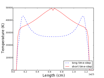
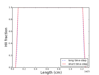
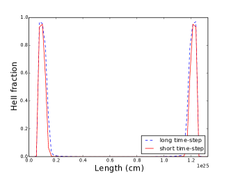
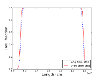
Figure 1: Temperature and ionization fraction results at $10^{7}$ years for two simulations using different (constant) time-steps. Blue dashed lines: long time-step ($10^{7}$ years); red solid lines: short time-step ($10^{-6}$ years). Top left panel: Temperature profile. Top right panel: HII fraction profile. Bottom left panel: HeII fraction profile. Bottom right panel: HeIII fraction profile. The cubic volume is 4.2 Mpc across and is divided into $60^{3}$ cells. A black body source with an ionizing photon rate $5\times 10^{56}$ s^-1 and temperature 100,000 K is located at the centre of the volume. The initial temperature is 100 K and both hydrogen and helium are fully neutral. The plots show the values along a line containing the source location. The simulation using a long time-step severely underestimates the temperature in the centre of the HII region and overestimates the temperature at the location of the ionization front. The small dip near the source in the temperature result for the short time-step case is caused by the same effect.

3 Adaptive time-step algorithm

3.1 Time-step criteria

The optimal size of the time-step will depend on the state of simulation at the start of the simulation step. It can thus not be set at the start of the simulation but needs to be calculated on the fly. This actually requires performing part of the calculation to obtain the rates of change of the quantities at hand (in our case ionization fraction and temperature) and use these to establish the optimal time-step for each cell. The smallest among these values should then be selected to be the time-step of the next simulation step.

Since the cause of the inaccurate temperature results lies in the fact that cells change their ionization state too much over the time-step, the obvious solution is to force ionization fronts not to proceed more than one cell within a time-step. This way all cells which become ionized in this time-step will experience the optically thick heating phase.

To implement this we introduce a free parameter $f$ so that the change in $x_{\mbox{\scriptsize{HII}}}$, $\Delta x_{\mbox{\scriptsize{HII}}}$, is at most $1/f$ in each time-step. Note that this is an absolute condition, not a relative one. A relative condition would limit the quantity $\Delta x_{\mbox{\scriptsize{HII}}}/x_{\mbox{\scriptsize{HII}}}$. Mackey (2012) investigated the merits of absolute and relative constraints on the change in ionized fractions when setting the time-step and concluded that absolute constraints are more efficient.

We find the required time-step $\Delta t$ by solving the ionization equation (see equation (12) in Mellema et al. (2006))

$$\Delta t=\frac{1}{\Gamma^{\mbox{\scriptsize{HI}}}}\ln\frac{x_{\mbox{\scriptsize{HII}}}^{\mbox{\scriptsize{begin}}}-1}{x_{\mbox{\scriptsize{HII}}}^{\mbox{\scriptsize{final}}}-1}\,,$$ (18)

imposing the result

$$x^{\mbox{\scriptsize{final}}}_{\mbox{\scriptsize{H{\sc II}}}}=\min\{x^{\mbox{\scriptsize{begin}}}_{\mbox{\scriptsize{H{\sc II}}}}+1/f,1-\epsilon\}\,,$$ (19)

where $\mathbin{x^{\mbox{\scriptsize{begin}}}_{\mbox{\scriptsize{H{\sc II}}}}}$ and $\mathbin{x^{\mbox{\scriptsize{final}}}_{\mbox{\scriptsize{H{\sc II}}}}}$ are the ionized hydrogen fractions at the beginning and the end of the simulation step. In this $\epsilon$ is an arbitrarily small number introduced to stop the time-step from diverging when $x^{\mbox{\scriptsize{final}}}_{\mbox{\scriptsize{H{\sc II}}}}\rightarrow 1$. We then adopt the minimum of all the $\Delta t$’s as the time-step for the current simulation step.

The complication we face is that the $\Gamma$ and $\mathcal{H}$ values depend on the choice for the time-step. In order to determine the optimal time-step we thus need to first choose a time-step, determine the $\Gamma$ and $\mathcal{H}$ values and then find the optimal time-step for these values. In principle one would need to iterate this process. However, as we saw above, although the value for $\mathcal{H}$ depends sensitively on the time-step, the values for the $\Gamma$ do not. We therefore do not use the $\mathcal{H}$ values for estimating the optimal time-step, but only the $\Gamma$ values. The helium photo-ionization rates $\Gamma^{\mbox{\scriptsize{HeI}}}$ and $\Gamma^{\mbox{\scriptsize{HeII}}}$ are not considered since we found that time-steps estimated from $\Gamma^{\mbox{\scriptsize{HI}}}$ alone suffice to get an accurate temperature evolution. We experimented with different time-steps and found that a reasonable optically thick $\langle\mathcal{H}\rangle$ is estimated if $x_{\mbox{\scriptsize{H{\sc I}}}}$ does not change substantially during the time-step. The appropriate value of $f$ depends somewhat on the problem and the required accuracy. However, for typical IGM gas densities values we recommend values in the range $2\leq f\leq 5$. Reasonable values for the optically thin $\langle\mathcal{H}\rangle$ can be obtained regardless of the time-step.

Since only ionization front cells require a more strict time-step in order to obtain accurate heating rates, we do not need to evaluate the photo-ionization rate $\Gamma^{\mbox{\scriptsize{HI}}}$ for all cells. It suffices to calculate them for the cells which are currently being photo-ionized or in other words the ionization front cells (ICs). Furthermore, since a simulation volume can contain several sources of ionizing photons, when evaluating the effect of a single source we should not consider all ICs but only the ones which are nearest to this source. These we will designate as nearest ionization front cells (NICs).

Finding the values of $\Gamma^{\mbox{\scriptsize{HI}}}$ at the locations of the NICs in principle requires ray-tracing from the source to those locations in order to find the optical depths. However, we do not need such accuracy for the optical depths if we only want to derive a time-step. Instead, we find the locations of the NICs and assume that the optical depths at the NIC are dominated by the NICs themselves, i.e. if $\tau_{\mathrm{NIC}}$ is the optical depth from the source to the NIC and $\Delta\tau_{\mathrm{NIC}}$ is the optical depth of the NIC itself, we assume that $\Delta\tau_{\mathrm{NIC}}\gg\tau_{\mathrm{NIC}}$. In this case, the only thing required is to find the location of the NICs. Note that our time-step estimate also works well in high resolution simulations when $\Delta\tau_{\mathrm{NIC}}\sim\tau_{\mathrm{NIC}}\ll 1$. This is because the $\Gamma^{\mbox{\scriptsize{HI}}}$ estimate always works well in the optically thin regime $(\tau_{\mathrm{NIC}}\ll 1)$ and for optically thin cells $(\Delta\tau_{\mathrm{NIC}}\ll 1)$. The next sections explain how we find the locations of the NICs for the case of a single source.

3.2 Pyramidal ray tracing framework

Identifying the NICs for a given source is not trivial. The obvious choice for this task is a ray-tracing method. However, the short characteristics ray tracing method used by C²-Ray is not useful for this purpose as it efficiently integrates quantities in all directions but does not record ‘events’ along a particular direction. For such a task, a long characteristics method is the more natural choice.

Consider a volume of $\mathbin{P^{3}}$ cells. In its simplest form long characteristics ray tracing would require tracing $\mathbin{6P^{2}}$ rays to cover all cells in the volume. Along each ray one would need to identify the ICs, calculate their distances to the source and compare these in order to identify the NIC for that ray. Since the density of rays close to the source will be high, the same NICs could be traversed by several rays, leading to redundant work. Such a brute force approach would be highly inefficient.

Here we introduce a new long characteristics ray-tracing method for identifying the NICs for a source. Our method relies on two key ideas. First, we trace the lowest possible number of rays from a source to identify all NICs. Second, we avoid calculation and comparison of distances by storing the ICs in a sorted list such that for a given ray the IC with the smallest index is the NIC. The combination of these two ideas leads to a very efficient method. Below we describe the algorithm in detail for the case of one source. The repeated use of the method works well for the case of multiple sources.

First, we identify all the ICs in the simulation box. We define neutral as $x_{\mbox{\scriptsize{HI}}}\geq 1/(1+f)$ and ionized otherwise. Note that $f$ is the same parameter as defined in Section 3.1. We then define the set of all the ionized cells to be $\mathbb{I}$. We define another set of cells $\mathbb{IB}$ which contains the union of all the $3\times 3\times 3$ cubes of cells in which the centres of the cubes are ionized cells. The $\mathbb{IB}$ cells which do not belong to $\mathbb{I}$ are the ICs. That is to say, the set $\mathbb{B}\equiv\mathbb{IB}\backslash\mathbb{I}$ is the set of ICs.

Next we need to establish a coordinate centre for the ray tracing. We define the source cell to be the origin of this coordinate system. If periodic boundary conditions are assumed, we translate the coordinate system so that the source is located in the centre of the simulation volume. Since we do not trace radiation which leaves the volume, these are not periodic boundary conditions in a formal sense. However, since this procedure makes the horizon for the radiation different for each source, it does create a pseudo-periodic character for the simulation. For transmissive boundary conditions we do not change the relative position of sources within the simulation volume.

In this coordinate system, the coordinates $(i,j,k)$ of the simulation box for both cases thus follow the constraints $-M_{x}^{-}\leq i\leq M_{x}^{+}$, $-M_{y}^{-}\leq j\leq M_{y}^{+}$ and $-M_{z}^{-}\leq k\leq M_{z}^{+}$, where for example $M_{x}^{-}$ is the distance in terms of cell width from the source to edge of the simulation volume along the negative $x$-axis. Note that our current ray-tracing scheme works only on a fixed, regularly spaced grid. Further improvements are required to use it with an adaptive mesh refinement grid.

Using this coordinate system we then construct 24 pyramidal components by first dividing the simulation volume into 8 octants (see Figure 2 for the case of a source in the centre of the simulation volume) and next dividing each octant into 3 pyramidal components (see Figure 3 and 4, also for a centrally located source). A pyramidal component consists of a rectangular base and a vertex where the source lies. All the pyramidal components have the source at their vertices.

There are two reasons for setting up such a pyramidal decomposition of the grid. First, a pyramidal component is the smallest repeated sub-domain unit in our ray-tracing scheme. The problem is thus reduced to identifying NICs in one pyramidal component. Simply stated, if the NICs all lie at the tip of the pyramid, there is no need to trace the rest of the pyramid. Second, the pyramidal ray-tracing process is highly parallelizable as the ray-tracing in one pyramidal component is independent of the ray-tracing in the other ones.

To distinguish the different components we introduce a nomenclature for the pyramidal components. This takes the form $[A,B,C]$, where $A$ indicates the direction of the primary axis, $B$ indicates the direction of the secondary axis and $C$ indicates the direction of the tertiary axis. For example for the octant of positive $x$, $y$ and $z$ coordinates, there are three pyramidal components, one with the primary axis along the $x$ axis, $[+x,+y,+z]$, one with the primary axis along the $y$ axis, $[+y,+x,+z]$ and one with the primary axis along the $z$ axis, $[+z,+y,+x]$. If in Fig. 4 $x$, $y$ and $z$ axes run along the blue, green and red sides of the cube, these three pyramidal components correspond to the blue, green and red pyramids, respectively. This nomenclature not only defines the pyramidal components but is also useful to describe the ray-tracing within each component in a coordinate independent way.

Table 1 defines the full set of pyramidal components. The first column shows the names of the 24 pyramidal components. Each component consists of a set of cells $(i,j,k)$’s. The parameters $i$, $j$ and $k$ of a pyramidal component satisfy the following bounds, $l_{i}\leq i\leq u_{i}$, $l_{j}\leq j\leq u_{j}$ and $l_{k}\leq k\leq u_{k}$. The functional values of $l_{i},u_{i},l_{j},u_{j},l_{k},u_{k}$ need not to be constants. They are defined according to the second to the seventh columns of Table 1. We note that with this definition of the pyramidal components, they do not necessarily form a complete pyramid. That is, some part of the volume may be cropped so that the base is not necessarily a square.

component	$l_{i}$	$u_{i}$	$l_{j}$	$u_{j}$	$l_{k}$	$u_{k}$
$[+x,+z,+y]$	0	$M_{x}^{+}$	0	$\min\{i,M_{y}^{+}\}$	0	$\min\{i,M_{z}^{+}\}$
$[+y,+x,+z]$	0	$\min\{j,M_{x}^{+}\}$	0	$M_{y}^{+}$	0	$\min\{j,M_{z}^{+}\}$
$[+z,+y,+x]$	0	$\min\{k,M_{x}^{+}\}$	0	$\min\{k,M_{y}^{+}\}$	0	$M_{z}^{+}$
$[-x,+z,+y]$	$-M_{x}^{-}$	0	0	$\min\{-i,M_{y}^{+}\}$	0	$\min\{-i,M_{z}^{+}\}$
$[+y,-x,+z]$	$\max\{-j,-M_{x}^{-}\}$	0	0	$M_{y}^{+}$	0	$\min\{j,M_{z}^{+}\}$
$[+z,+y,-x]$	$\max\{-k,-M_{x}^{-}\}$	0	0	$\min\{k,M_{y}^{+}\}$	0	$M_{z}^{+}$
$[+x,+z,-y]$	0	$M_{x}^{+}$	$\max\{-i,-M_{y}^{-}\}$	0	0	$\min\{i,M_{z}^{+}\}$
$[-y,+x,+z]$	0	$\min\{-j,M_{x}^{+}\}$	$-M_{y}^{-}$	0	0	$\min\{-j,M_{z}^{+}\}$
$[+z,-y,+x]$	0	$\min\{k,M_{x}^{+}\}$	$\max\{-k,-M_{y}^{-}\}$	0	0	$M_{z}^{+}$
$[-x,+z,-y]$	$-M_{x}^{-}$	0	$\max\{i,-M_{y}^{-}\}$	0	0	$\min\{-i,M_{z}^{+}\}$
$[-y,-x,+z]$	$\max\{j,-M_{x}^{-}\}$	0	$-M_{y}^{-}$	0	0	$\min\{-j,M_{z}^{+}\}$
$[+z,-y,-x]$	$\max\{-k,-M_{x}^{-}\}$	0	$\max\{-k,-M_{y}^{-}\}$	0	0	$M_{z}^{+}$
$[+x,-z,+y]$	0	$M_{x}^{+}$	0	$\min\{i,M_{y}^{+}\}$	$\max\{-i,-M_{z}^{-}\}$	0
$[+y,+x,-z]$	0	$\min\{j,M_{x}^{+}\}$	0	$M_{y}^{+}$	$\max\{-j,-M_{z}^{-}\}$	0
$[-z,+y,+x]$	0	$\min\{-k,M_{x}^{+}\}$	0	$\min\{-k,M_{y}^{+}\}$	$-M_{z}^{-}$	0
$[-x,-z,+y]$	$-M_{x}^{-}$	0	0	$\min\{-i,M_{y}^{+}\}$	$\max\{i,-M_{z}^{-}\}$	0
$[+y,-x,-z]$	$\max\{-j,-M_{x}^{-}\}$	0	0	$M_{y}^{+}$	$\max\{-j,-M_{z}^{-}\}$	0
$[-z,+y,-x]$	$\max\{k,-M_{x}^{-}\}$	0	0	$\min\{-k,M_{y}^{+}\}$	$-M_{z}^{-}$	0
$[+x,-z,-y]$	0	$M_{x}^{+}$	$\max\{-i,-M_{y}^{-}\}$	0	$\max\{-i,-M_{z}^{-}\}$	0
$[-y,+x,-z]$	0	$\min\{-j,M_{x}^{+}\}$	$-M_{y}^{-}$	0	$\max\{j,-M_{z}^{-}\}$	0
$[-z,-y,+x]$	0	$\min\{-k,M_{x}^{+}\}$	$\max\{k,-M_{y}^{-}\}$	0	$-M_{z}^{-}$	0
$[-x,-z,-y]$	$-M_{x}^{-}$	0	$\max\{i,-M_{y}^{-}\}$	0	$\max\{i,-M_{z}^{-}\}$	0
$[-y,-x,-z]$	$\max\{j,-M_{x}^{-}\}$	0	$-M_{y}^{-}$	0	$\max\{j,-M_{z}^{-}\}$	0
$[-z,-y,-x]$	$\max\{k,-M_{x}^{-}\}$	0	$\max\{k,-M_{y}^{-}\}$	0	$-M_{z}^{-}$	0

Table 1: Definitions of the 24 pyramidal components. The first column contains the names of the pyramidal components. Each set of three constitutes one of the eight octants, see Fig. 2. The three pyramidal components for one octant are illustrated in Fig. 3. Columns 2 through 7 list the coordinates defining each pyramidal component: lower bound of $\mathbin{x}$, upper bound of $\mathbin{x}$, lower bound of $\mathbin{y}$, upper bound of $\mathbin{y}$, lower bound of $\mathbin{z}$, upper bound of $\mathbin{z}$, respectively. To see if a point $(i,j,k)$ is part of a given pyramidal component, check whether the values of $i$, $j$ and $k$ fall within the listed bounds.

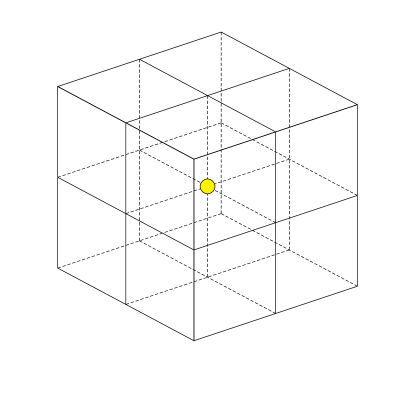
Figure 2: The simulation volume is decomposed into 8 octants. The yellow spot indicates the position of the source. Note that for simplicity this graphical illustration only shows the case of the source being located in the centre of the volume. The domain decomposition for the case when the source does not lie in the centre of the volume follows the same principle.

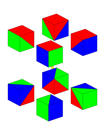
Figure 3: Each octant is further decomposed into 3 pyramidal components. Here we use red, green and blue for the different pyramidal components to easily distinguish them. Note that the source is located at the vertex of each of the 24 pyramidal components.

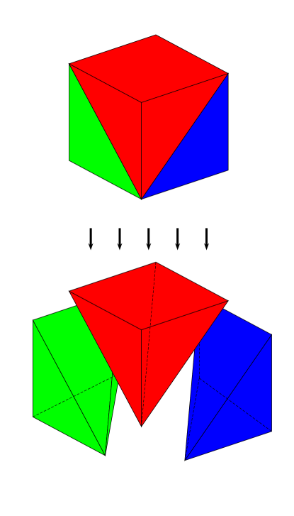
Figure 4: Detailed decomposition into pyramidal components.

Using the pyramidal decomposition of the volume, we construct the list of ICs as follows. Let the pyramidal component $[A,B,C]=[\pm a,\pm b,\pm c]$ have $\mathbin{N_{t}}$ ICs. The IC list has therefore size $N_{t}$. ’ We scan through the whole component cell by cell in a specific order. Starting from the source, we proceed to the next cell along the primary axis ($A$ direction). If an IC is encountered, we store its coordinates in the list of ICs using an ascending order of indices. After we have scanned the whole row, we move to the neighbouring row, which is parallel to the previous row but displaced in the direction of the secondary axis ($B$ direction). We perform the scanning of this row from the cell closest to the source, and then proceed to the next cell in the $A$ direction until we finish the whole row. We repeat this procedure until the first plane of cells has been scanned, after which we proceed to the next plane which is parallel to the first plane but displaced along the tertiary axis ($C$) direction. This second plane is scanned in the same way as the first one. We scan subsequent planes until all the cells of the pyramidal component have been scanned. After this the IC list stores the coordinates of the $N_{t}$ ICs in an order beneficial for the NIC identification method we describe in Section 3.3.

3.3 NIC identification

To find the NICs from the list of ICs for a given pyramidal component, we use the following algorithm. Let $M_{b}=\min\{M^{\pm}_{a},M^{\pm}_{b}\}$ and $M_{c}=\min\{M^{\pm}_{a},M^{\pm}_{c}\}$, where the $M^{\pm}_{a}$, $M^{\pm}_{b}$ and $M^{\pm}_{c}$ follow the signs of the pyramidal component $[A,B,C]=[\pm a,\pm b,\pm c]$. The base of the pyramidal component is a plane of $(M_{b}+1)\times(M_{c}+1)$ cells. We define the coordinates of these base cells as $(i_{\mbox{\scriptsize{secondary}}},i_{\mbox{\scriptsize{tertiary}}})$. The base cell closest to the source has coordinate $(0,0)$ and the base cell furthest from the source has coordinate $(\pm M_{\mbox{\scriptsize{b}}},\pm M_{\mbox{\scriptsize{c}}})$. In this $\pm M_{b}$ and $\pm M_{c}$ have the same signs as $B=\pm b$ and $C=\pm c$, respectively.

In our method, we send rays into a pyramidal component following the algorithm given in Section 3.4. The rays start from the source cell and pass through the planes that lie parallel to the base. We choose to indicate the direction of a ray with the coordinates of its crossing point with the base plane $(i_{\mbox{\scriptsize{secondary}}},i_{\mbox{\scriptsize{tertiary}}})$ which is not necessarily a 2-tuple of integers. In addition, the directions of rays are not constrained by the base plane of $(M_{b}+1)\times(M_{c}+1)$ cells, but by a slightly larger plane of $(M^{\pm}_{a}+1)\times(M^{\pm}_{a}+1)$ cells. One can imagine that this larger plane and the position of the source form a complete pyramid which includes the pyramidal component $[A,B,C]$. Both the complete pyramid and the pyramidal component $[A,B,C]$ span the same solid angle from their vertices.

We check for each ray if it passes through the ICs stored in the IC list in an ascending order. That is, we start from the first element of the IC array, and then the second, and so on. Due to the order in which the ICs are stored, the first IC to pass this test is the NIC.

For a ray to pass through a cell, it has to pass through a cell face parallel to the base plane, either the plane facing the source or the plane facing away from the source, or both. For an IC with centre coordinates $(i_{x},i_{y},i_{z})$ located in the pyramidal component $[A,B,C]$ these two faces are defined by $j_{a}=i_{a}+\mbox{sgn}(A)/2$ (i.e. $a^{+}$ plane) and $j_{a}=i_{a}-\mbox{sgn}(A)/2$ (i.e. $a^{-}$ plane). We remind the reader that the variables $a\in\{x,y,z\}$ and $A=\pm a$ follow from the primary axis and its sign of the pyramidal component, so for example in pyramidal component $[-y,x,z]$, $a=y$ and therefore the $a^{+}$ plane is defined by $j_{y}=i_{y}-1/2$.

Given the location of these two planes, the ray equation for a ray $(i_{\mbox{\scriptsize{secondary}}},i_{\mbox{\scriptsize{tertiary}}})$, provides us with the other two coordinates of the location where the ray crosses these planes, denoted as $j_{b}$’s and $j_{c}$’s (in the example given above these would be $j_{x}$ and $j_{z}$). Figure 5 and 6 illustrate how a ray crosses an IC at the $a^{-}$ and $a^{+}$ planes and also show the geometrical meaning of the different coordinates. To establish whether the ray crosses the IC we just need to compare these to the coordinates of the IC. If the ray passes through this IC, at least one of the following two conditions has to be satisfied.

1. The ray traverses into the IC at the $a^{-}$ plane if and only if $|i_{b}-j_{b}(\mbox{$a^{-}$})|\leq 1/2$ and $|i_{c}-j_{c}(\mbox{$a^{-}$})|\leq 1/2$.

2. The ray traverses into the IC at the $a^{+}$ plane if and only if $|i_{b}-j_{b}(\mbox{$a^{+}$})|\leq 1/2$ and $|i_{c}-j_{c}(\mbox{$a^{+}$})|\leq 1/2$.

Since the first IC to pass the test is the NIC, we then stop the NIC identification procedure for this ray and proceed to the next ray. We explain the selection of this next ray in Section 3.4.

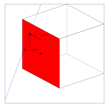
Figure 5: A ray traverses an IC with centre coordinates $(i_{x},i_{y},i_{z})$ at the $a^{-}$ plane (the red area). The entry point $(j_{a},j_{b},j_{c})$ is indicated by a dot. The center of the IC’s $a^{-}$ face $(j_{a},i_{b},i_{c})$ is indicated by a crosshatched circle. The distances between the entry point and the cell centre, projected along the $b$ and $c$ directions, are shown by the black arrows and the quantities next to the black arrows.

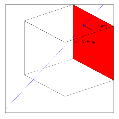
Figure 6: Same as Figure 5 but for the $a^{+}$ plane.

3.4 Ray updating algorithm

The first ray considered is $(i_{\mbox{\scriptsize{secondary}}},i_{\mbox{\scriptsize{tertiary}}})=(0,0)$. However, in order to minimize the number of rays to check we do not step through all possible values $(i_{\mbox{\scriptsize{secondary}}},i_{\mbox{\scriptsize{tertiary}}})$ but instead select the next ray depending on whether the previous one traversed a NIC or not. If the previous ray $(i_{\mbox{\scriptsize{secondary}}},i_{\mbox{\scriptsize{tertiary}}})$ did not cross an IC, the next ray $(i^{\prime}_{\mbox{\scriptsize{secondary}}},i_{\mbox{\scriptsize{tertiary}}})$ will simply have $i^{\prime}_{\mbox{\scriptsize{secondary}}}=i_{\mbox{\scriptsize{secondary}}}+\mbox{sgn}(B)$. If it did, the selection of the next ray depends on the location of the entry point into the IC. This entry point lies on one of the faces of the NIC facing the source, either the front, the side, or the bottom face, as shown in Figure 7. The bottom face is divided into two parts (labelled 1 and 2) to aid the ray-updating algorithm. From the ray equation of the ray $(i_{\mbox{\scriptsize{secondary}}},i_{\mbox{\scriptsize{tertiary}}})$ we can check which face the previous ray passed through.

1. If the previous ray entered through the front face, then the intersection $(j_{x},j_{y},j_{z})$ of the ray to the plane $j_{a}=i_{a}-\mbox{sgn}(A)/2$ satisfied $|i_{b}-j_{b}|\leq 1/2$ and $|i_{c}-j_{c}|\leq 1/2$.

2. If the previous ray entered through the side face, then the intersection $(j_{x},j_{y},j_{z})$ of the ray to the plane $c=i_{c}-\mbox{sgn}(C)/2$ satisfied $|i_{a}-j_{a}|\leq 1/2$ and $|i_{b}-j_{b}|\leq 1/2$.

3. If the previous ray entered through the bottom face, then the intersection $(j_{x},j_{y},j_{z})$ of the ray to the plane $b=i_{b}-\mbox{sgn}(B)/2$ satisfied $|i_{a}-j_{a}|\leq 1/2$ and $|i_{c}-j_{c}|\leq 1/2$.

   1. For the same ray, if its intersection $(k_{x},k_{y},k_{z})$ to the plane $a=i_{a}-\mbox{sgn}(A)/2$ satisfied $|i_{c}-k_{c}|\leq 1/2$, it entered through bottom face 1.

   2. Otherwise, it entered through bottom face 2.

We then choose the next ray such that it will touch on the verge (green line in Figure 7) of the traversed IC $(i_{x},i_{y},i_{z})$. This is achieved by setting the value of $i^{\prime}_{\mbox{\scriptsize{secondary}}}$ according to the following rules:

1. If the previous ray passed through the front face or the bottom face 1, the new ray is selected to touch the line $\frac{a}{i_{a}-\mbox{\scriptsize{sgn}}(A)/2}=\frac{b}{i_{b}+\mbox{\scriptsize{sgn}}(B)/2}$. This implies $i^{\prime}_{\mbox{\scriptsize{secondary}}}=\pm M^{\pm}_{a}\frac{i_{b}+\mbox{\scriptsize{sgn}}(B)/2}{i_{a}-\mbox{\scriptsize{sgn}}(A)/2}$. Both $\pm$ follow the sign of $A=\pm a$.

2. If the previous ray passed through the side face or the bottom face 2, the new ray is selected to touch the line $\frac{b}{i_{b}+\mbox{\scriptsize{sgn}}(B)/2}=\frac{c}{i_{c}-\mbox{\scriptsize{sgn}}(C)/2}$. This implies $i^{\prime}_{\mbox{\scriptsize{secondary}}}=i_{\mbox{\scriptsize{tertiary}}}\frac{i_{b}+\mbox{\scriptsize{sgn}}(B)/2}{i_{c}-\mbox{\scriptsize{sgn}}(C)/2}$.

If the new ray $(i^{\prime}_{\mbox{\scriptsize{secondary}}},i_{\mbox{\scriptsize{tertiary}}})$ falls outside the angular range of the pyramidal component, i.e. if $|i^{\prime}_{\mbox{\scriptsize{secondary}}}|>M^{\pm}_{a}+1$, we skip NIC identification for this ray and proceed to the ray $(0,i_{\mbox{\scriptsize{tertiary}}}+\mbox{sgn}(C))$, the first ray of the next slice. The ray updating terminates once the ray coordinates reach $(i^{\prime\prime}_{\mbox{\scriptsize{secondary}}},i^{\prime\prime}_{\mbox{\scriptsize{tertiary}}})$ where $|i^{\prime\prime}_{\mbox{\scriptsize{tertiary}}}|>M^{\pm}_{a}+1$. This ray updating algorithm ensures that we use the minimum number of rays required to trace all the NICs.

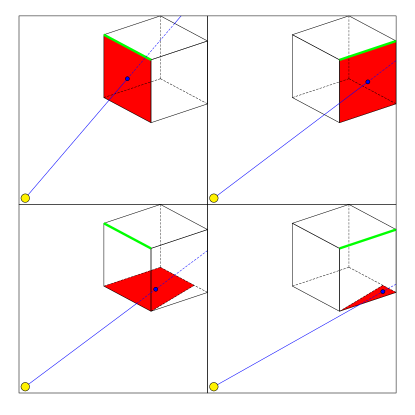
Figure 7: A ray enters into a cell through one of the four faces. Top-left: the ray passes through front face. Top-right: the ray passes through side face. Bottom-left: the ray passes through bottom face 1. Bottom-right: the ray passes through bottom face 2. The thick green line in each subplot indicates the verge of the cell through which the next ray will pass.

3.5 IC removal in the array

The ray-tracing proceeds slice by slice in a pyramidal component, i.e. the unity increment of $|i_{\mbox{\scriptsize{tertiary}}}|$ described in the last paragraph of the previous section implies proceeding to the neighbouring slice. After a slice has been scanned, the list of ICs can contain ICs from this slice which are not NICs. Since these ICs will never become NICs for other slices, it is best to remove them from the list of ICs so that they no longer need to be considered.

Figure 8 shows an illustration of NIC identification and the removal of the other ICs in one pyramidal component. In the top left panel of Figure 8, a pyramidal component contains a number of ICs (pink cells). We consider the case of multiple sources of ionization so that there are ionized regions away from the source being considered. The source is located at the vertex position. The ICs are stored in the IC list in the order explained in Section 3.2. The top right panel of Figure 8 shows how the first few rays are sent through the first slice of cells. The NIC identification procedure (Section 3.3) identifies the NICs, indicated by the green cells. The bottom left panel of Figure 8 shows how the ICs which are not NICs from the first slice are removed from the list of ICs to avoid their use in the NIC identification procedure for the subsequent slices. The bottom right panel of Figure 8 shows the end stage of the ray-tracing method: the IC list only stores NICs which are then used to estimate the adaptive time-step for the next evolution cycle. The total number of rays used in this example is 53 and the number of base cells is 100, illustrating the efficiency of our ray selection algorithm.

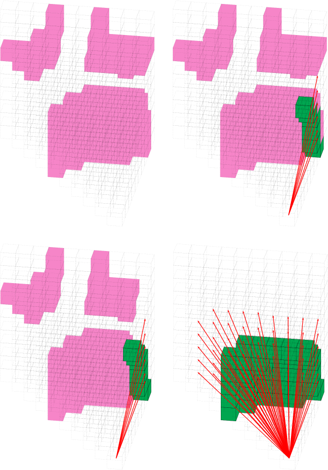
Figure 8: Top left panel: A graphical example of a pyramidal component which contains a number of ICs (pink cells). The source is located at the vertex position. Top right panel: a series of rays (red arrows) are sent through the first slice following the procedure specified in Section 3.4. The NICs are shown in green and the other ICs in the first slice remain pink. Bottom left panel: The other ICs (pink cells) of the first slice are removed as described in Section 3.5. Bottom right panel: At the end of the procedure, all the slices in the pyramidal components have been scanned by rays. All NICs (green cells) have been identified and all other ICs (pink cells) have been removed.

3.6 Multiple-source treatment

The previous sections (3.2 – 3.5) have explained in detail the adaptive time-step algorithm for the single-source case. In the multiple-source case, we repeat the same procedure to obtain photo-ionization rates of NICs for each source. The sum of the photo-ionization rates contributed by all sources is then used to calculate the time-step $\Delta t_{k}$ for each NIC $k$. The adaptive time-step $\Delta t$ is the minimum of all $\Delta t_{k}$’s.

4 Asynchronized evolution

4.1 Introduction

In most types of simulations all computational cells use the same time-step, be it a constant time-step or an adaptive time-step. Section 3 outlined how the photo-heating rates $\mathcal{H}$’s of all cells can be calculated accurately using an adaptive time-step. The main problem with this approach is that the adaptive time-step is almost always much smaller than the recombination timescale, thus making the simulation more expensive. However, the photo-heating events occur only in particular cells in the simulation volume, so not all the cells necessarily need to use this relatively small time-step for an accurate photo-heating calculation. Consider for example an ionized cell which is close to thermal and ionization equilibrium. In this cell the evolution of the ionization and temperature will be slow and the optical depths across this cell will essentially be constant. Using a relatively short time-step on these ionized cells is a waste of computational resources.

Asynchronous evolution is the application of different time-steps to different cells. The general idea is that cells which are close to equilibrium use relatively long time-steps while the rest use relatively short time-steps. This approach will dedicate most of the computational resources to the cells that require it thus saving a substantial amount of computational time.

For an expanding HII region, there are three types of cells. Inside the HII region there are the ionized cells which are close to equilibrium. Next there are the ionization front cells which are far from equilibrium. Beyond the ionization front lie the neutral cells which may or may not be in equilibrium and thus require careful consideration. For a long time-step, the ionization front may advance substantially into the neutral region and thus the cells that were neutral and in equilibrium at the start of the time-step may not remain so during the time-step. Furthermore, if the source contains sufficiently energetic photons these will penetrate far beyond the ionization front and start to heat and ionize the neutral material, in some cases establishing an ionization front which is as broad as the entire computational domain.

For these reasons we decide to only consider the ionized cells to be in equilibrium and to group the neutral cells together with the ionization front cells as non-equilibrium cells. This means that when the ionized regions cover only a small fraction of the computational domain, the gain from using asynchronous evolution will be small. Large gains are only achieved once the ionized regions have grown substantially.

Both reasons for including the neutral cells in the set of non-equilibrium cells can in principle be dealt with, for example by forecasting the extent by which the ionized regions will grow during a time-step and measuring the photo-rates in the neutral cells. However, we postpone an exploration of this to future work.

4.2 Asynchronous evolution algorithm

Let us assume that we start our simulation at $t=0$ and want to know the state of our computational domain at a time $\Delta t$. We categorize the cells into three sets.

• $\mathcal{L}$ is the set of ionized cells which are in thermal equilibrium and their clocks are $t<\Delta t$ (i.e. ionized cells).

• $\mathcal{S}$ is the set of non-$\mathcal{L}$ cells and their clocks clocks are $t<\Delta t$ (i.e. ionization front and neutral cells).

• $\mathcal{E}$ is the set of cells whose clocks are $t=\Delta t$ (i.e. all cells at the end of the simulation step).

The criterion for thermal equilibrium of the ionized cells is discussed in Section 4.3.

At the start of the simulation, all the cells’ clocks are synchronized at $t=0$. We identify which cells belong to sets $\mathcal{L}$ or $\mathcal{S}$. The $\mathcal{L}$ cells are assigned a time-step $\Delta t$ while the $\mathcal{S}$ cells are assigned a time-step $\Delta t_{1}$ where $\Delta t_{1}$ is the adaptive time-step of the first evolution stage. In the first evolution stage, only $\mathcal{S}$ cells are updated and their clocks are set to $t=\Delta t_{1}$. The $\mathcal{L}$ cells are not updated and so their clocks remain $t=0$.

Next, we identify the new sets of $\mathcal{L}$ cells and $\mathcal{S}$ cells. The new $\mathcal{L}$ cells are assigned a time-step $\Delta t-\Delta t_{1}$ while $\mathcal{S}$ cells are assigned a time-step $\Delta t_{2}$ where $\Delta t_{2}$ is the adaptive time-step of the second evolution stage. Also in the second evolution stage, only $\mathcal{S}$ cells are updated and their clocks reach $t=\Delta t_{1}+\Delta t_{2}$. The $\mathcal{L}$ cells keep their clocks at $t=0$. Note that the $\mathcal{L}$ cells from the first stage are assigned a time-step $\Delta t$ while the those identified in the second stage are assigned a time-step $\Delta t-\Delta t_{1}$.

This procedure is repeated until all the clocks of the $\mathcal{S}$ cells from the previous stage reach $t=\Delta t$. In the other words, the procedure is repeated until the first $\mathcal{E}$ cells appear. Only after this we apply the different assigned time-steps to the ${\mathcal{L}}$ cells. This final stage is performed simultaneously for all ${\mathcal{L}}$ cells. With this all cells have become $\mathcal{E}$ cells with their clocks synchronized at $t=\Delta t$.

For the evolution of $\mathcal{S}$ cells, we calculate the photo-rates only for the $\mathcal{S}$ cells contributed by each source. The standard iterative method is used to get converged results for the multiple sources (see Friedrich et al., 2012). For the evolution of the $\mathcal{L}$ cells, we calculate the photo-rates only for the $\mathcal{L}$ cells and perform just one iteration on them and ignore the convergence issue. This is acceptable since for cells in both ionization and thermal equilibrium, further evolution does not produce fluctuating evolution results during several iterations.

Figure 9 shows an example of applying asynchronous evolution on a simulation volume. All the neutral cells are shown as white and they are all classified as $\mathcal{S}$ cells. Ionized cells are shown as pink or purple, depending on if they are newly identified $\mathcal{L}$ cells or previously identified $\mathcal{L}$ cells. As the ionized bubbles grow, more and more cells become $\mathcal{L}$ cells, which consume less computational resources. When the simulation volume is close to fully ionized, the computational costs to evolve it further are substantially reduced.

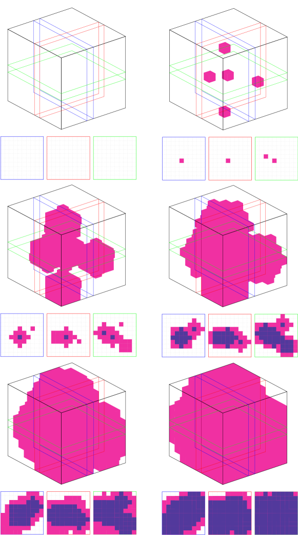
Figure 9: An example of asynchronous evolution. White: neutral $\mathcal{S}$ cells. Pink: newly identified $\mathcal{L}$ cells. Purple: previously identified $\mathcal{L}$ cells. Three slices through the source are shown separately. From top to bottom, from left to right shows the asynchronous evolution during five time-steps.

4.3 Criteria for thermal equilibrium

We need to define a good criterion of thermal equilibrium to assign cells to set $\mathcal{L}$. The best criterion would be one that is based on the values of the rates, as equilibrium is a state in which all rates are balanced. However, since it is the rates which we are trying to determine, we do not have access to them. Furthermore, their values may change over the period of a time-step.

As explained in Section 4.1 we only consider the ionized cells to be in equilibrium and hence a criterion based on the neutral fraction in a cell may be useful. Experiments show that this is indeed the case although the precise criterion is found to depend on the nature of the sources. Hard photons, for example, are able to change the thermal state of cells containing only trace amounts of photon absorbers. To define appropriate criteria, we have experimented with a range of different sources. For example, we have found that if the sources have black body spectra with a temperature of $T=50000K$ (an approximation of star-forming galaxies), letting cells which have $x_{\mbox{\scriptsize{HI}}}\leq 1\times 10^{-4}$ belong to set $\mathcal{L}$ and otherwise belong to set $\mathcal{S}$, gives satisfactory results. If the sources have power-law spectra with a spectral index of $1.5$ (an approximation of quasars where the emission is dominated by an accreting black-hole), letting cells which have $x_{\mbox{\scriptsize{HI}}}\leq 1\times 10^{-4}$ and $x_{\mbox{\scriptsize{HeII}}}\leq 1\times 10^{-4}$ belong to set $\mathcal{L}$ and otherwise belong to set $\mathcal{S}$, gives reasonable results.

These criteria based on the ionization fractions are only approximate and other options, such as using rates from previous time-steps, may be worth exploring in future work.

We would like to point out that our asynchronous evolution strategy works even when some of the ionized cells start recombining, for example in a radiation hydrodynamic simulation or one where sources can turn off. The reason is that the recombining cells evolve on a timescale set by the recombination time and can therefore be evolved with a long time-step as recombination times are typically much longer than ionization times.

5 Parallelization strategy

The performance of C²-Ray benefits from a high degree of parallelization. Its computational efficiency scales linearly with the number of cores used as long as the number of sources is larger than the number of cores. This is particularly important for large scale reionization simulations as they require substantial amounts of computing time and a large amount of memory.

C²-Ray uses a hybrid parallelization scheme that makes use of both distributed memory parallelization (employing the Message Passing Interface (MPI) library) and shared memory parallelization (based on the application programming interface OpenMP). An example of the scalability of the hydrogen-only version can be found in figure 1 of Iliev et al. (2014). Also the new version presented here has several procedures in which the contribution from one source is calculated independently of the existence of other sources. These procedures are the optical depth calculation by short characteristics ray-tracing, the photo-rates calculation, the NIC identification and the adaptive time-step calculation. Therefore it is advantageous to parallelize these procedures over the sources where one MPI process deals with one source at a time.

After having looped through all the sources, the MPI processes communicate with each other to exchange information. Examples of this are the summation of the photo-rates from all the sources and obtaining the adaptive time-step $\Delta t$ by extracting the minimum one among the $\Delta t_{s}$’s where $s$ is the index of the sources.

Since most of the procedures in C²-Ray can be parallelized over the sources, it possesses a high scaling efficiency when there are many sources. Furthermore, because sources emit radially, the radiative properties of the cells depend only on their neighbouring cells which are closer to the source in the radial directions. Examples of this are the optical depth calculation and the NIC identification. For this reason, we can further parallelize the procedures by domain decomposition and assign the decomposed domains to different OpenMP threads.

Of the procedures which are suitable for OpenMP parallelization the domain decomposition of short-characteristics ray-tracing is eight-fold (the eight octants), the photo-rates calculation can be $\mathbin{P^{3}}$-fold where $\mathbin{P^{3}}$ is the number of cells in the simulation box, the NIC identification is twenty four-fold (the 24 pyramidal components) and the adaptive time-step calculation is $m$-fold where $m$ is the number of NICs. The asynchronous evolution of $\mathcal{L}$ and $\mathcal{S}$ cells are independent of other cells, which makes the evolution procedure parallelizable. If $\mathbin{r}$ cells evolve with the same time-step, we distribute these cells into $\mathbin{r\approx p\times q}$ equal parts where $p$ is the number of MPI processes and $q$ is the number of OpenMP threads of each process. The evolution procedure of each part is assigned to each thread and the results from the different MPI processes are exchanged afterwards.

We end this section by concluding that C²-Ray is a highly parallelized radiative transfer code. It can run on many different types of parallel machines with different distributed memory (any number of distributed memory cores) and shared memory (2, 4, 8, 16, 24 threads per core) configurations. For example, a configuration which contains any number of distributed memory processors less than the number of sources and $2^{i}$ or $24\times 2^{j}$ threads per processor will fully utilize the computational resources. This high scaling efficiency is one of the important advantages of C²-Ray.

6 C²-Ray algorithm

We summarize the updated C²-Ray algorithm in Figures 10 – 13. These show how C²-Ray deals with a given time step $\Delta t$ which is too large for a correct photo-heating rate calculation. Figure 10 shows the overall algorithm and Figures 11 to 13 show in more detail the stages of the adaptive time-step calculation, evolution of the $\mathcal{S}$ cells and evolution of the $\mathcal{L}$ cells.

In the entire algorithm, the clocks of the cells are important. At time $t$ the clocks in all cells are synchronized. At the end they are synchronized again, at time $t+\Delta t$. The adaptive time-step algorithm goes through a series of $n$ stages, each with its own optimal time-step $\Delta t_{i}$, $\Delta t=\sum_{i=1}^{n}\Delta t_{i}$ and the evolution during these stages is performed asynchronously. At stage $i$, the set of $\mathcal{S}$ cells is evolved with a time-step $\Delta t_{i}$. Accurate photo-heating rates are obtained using this time-step and the clocks of $\mathcal{S}$ cells are increased by $\Delta t_{i}$. The convergence criteria stated in Figure 12 is that the relative change of $x_{\mbox{\scriptsize{HI}}}$, $x_{\mbox{\scriptsize{HeI}}}$ and $x_{\mbox{\scriptsize{HeIII}}}$ compared to the previous evolution cycle have to be smaller than a specified tolerance. For all the work in this paper the value used is 0.01.

This process is repeated until the clocks of the last set of $\mathcal{S}$ cells reaches $t+\Delta t$. After this the set of $\mathcal{L}$ cells are evolved with longer time-steps $\Delta t-\sum_{i=1}^{m-1}\Delta t_{i}$, where $m$ is the number of the stage after which they were identified as $\mathcal{L}$ cells. At the end of the simulation step the clocks of all cells are synchronized again at $t+\Delta t$.

Figure 10: Overall algorithm of C²-Ray.

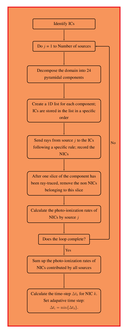
Figure 11: Adaptive time-step algorithm.

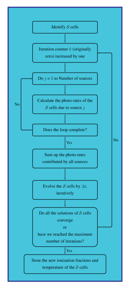
Figure 12: Asynchronous evolution algorithm of of $\mathcal{S}$ cells.

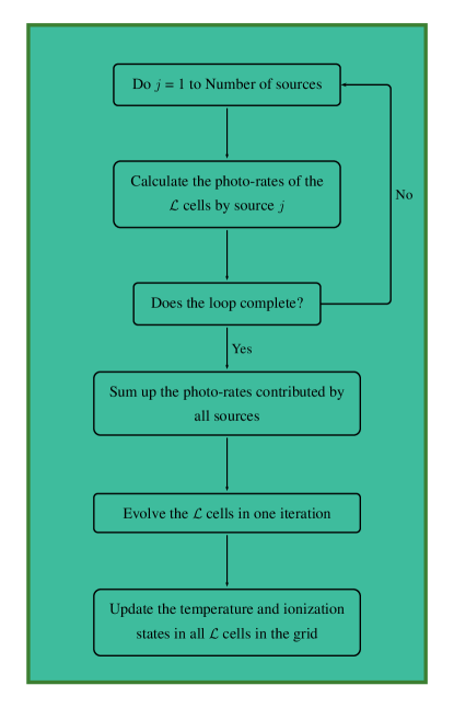
Figure 13: Asynchronous evolution algorithm of of $\mathcal{L}$ cells.

7 Tests

We perform four tests to evaluate and validate our new efficient photo-heating algorithm. In Tests 1 and 2, we consider a single source in a homogeneous density environment. In Test 3, we simulate multiple sources in a cosmological density field, using the standard set-up introduced by Iliev et al. (2006b). For these three tests we use both a constant time-step and our adaptive and asynchronous time-stepping approach. In Test 4, we compare C²-Ray results to those of another time-dependent photo-ionization code developed for supernova applications. The codes use different ionization and thermal solvers and this comparison thus serves to validate the results of C²-Ray.

7.1 Test 1 - Single source in a homogeneous environment

We start with a simple test to show the difference between the constant time-step and the adaptive time-step approach. The set-up is as follows. We assume a homogeneous density field of $n_{\mathrm{H}}=1.92\times 10^{-4}$ cm^-3 (the mean density at $z=9$ in a $\Omega_{\mathrm{b}}=0.043$, $H_{0}=70$ km s^-1 universe), temperature $T=100$ K and neutral fractions $x_{\mbox{\scriptsize{HI}}}=1$ and $x_{\mbox{\scriptsize{HeI}}}=1$. We put a single source at the center of a three-dimensional volume of size 4.2 Mpc. The resolution used is $30^{3}$. One model (1A) uses a black body source ($50000$ K) representing a Pop II galaxy and one model (1B) uses a power-law source $L_{\nu}\propto\nu^{-1.5}$ representing quasar emission. Both models assume an ionizing photon emission rate of $5\times 10^{55}$ s^-1. The constant time-step approach uses a time-step of $\Delta t=10$ Myr and the adaptive time-step approach uses $f=4$, meaning that the hydrogen ionized fraction can change by $\sim$25% in a time-step. The choice of $f=4$ is discussed below. This test does not use asynchronous evolution.

Figures 14 and 15 illustrate the evolution of the temperature along a line going through the source location. The different curves show the temperature profiles at 10 Myr (blue thin line), 40 Myr (red thicker line) and 80 Myr (green thickest line). The constant time-step approach (dashed lines) shows temperature spikes at several positions. These positions correspond to the positions of the ionization front after each time-step (10 Myr). These temperature spikes are the result of incorrect photo-heating rates, as explained in Section 2.3. The adaptive time-step approach (solid lines) shows smoother temperature profiles. These profiles peak at the source and decrease outward. The small wave-like structures are the result of slight deviations of photo-heating rate estimates from the correct photo-heating rate.

To determine which $f$ values produce accurate results, we explore a range of $f$ values (1 - 20) as well as a constant time-step simulation with a time-step of $5\times 10^{-4}$ Myr. We use the absolute value of the relative difference $p$ between the temperature fields of the $\Delta t=5\times 10^{-4}$ Myr and the adaptive time-step simulations as a measure of the accuracy of the latter. This quantity $p$ is calculated from

$$p=\frac{\sum_{x,y,z}|T_{a}(x,y,z)-T_{c}(x,y,z)|}{\sum_{x,y,z}T_{c}(x,y,z)},$$ (20)

where $T_{a}$ and $T_{c}$ are the temperature fields of adaptive and constant time-step approaches respectively. The results for $p$ of model (1A) and (1B) for output time 80 Myr and $1\leq f\leq 20$ are displayed in Figure 16. For $f=1$, the $p$ value is the highest for both models (7.12% for model (1A) and 8.24% for model (1B)). The $p$ value declines when $f$ increases. $p$ becomes less than $\sim$2% when $f>4$ and after that only slowly declines for larger $f$. We choose $f=4$ which corresponds to $p\sim 2\%$ to be the modest choice and the results for $f=4$ are shown in Figure 14 and 15.

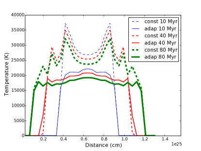
Figure 14: Test 1A: Thermal evolution of constant density with a black body source of 50000 K. Blue, red and green lines (of increasing thickness) are the results for $t=10$ Myr, $t=40$ Myr, $t=80$ Myr, respectively. Solid lines show the results from a simulation using the adaptive time-step approach and dashed lines from a simulation using a constant time-step of $\Delta t=10$ Myr. Note the wavy temperature profiles for the constant time-step model.

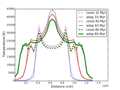
Figure 15: Same as Figure 14, but for test 1B: a power-law source with index 1.5.

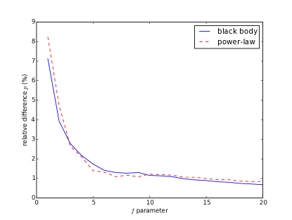
Figure 16: Absolute value of the relative difference $p$ between the results of Test 1 at time 80 Myr for the constant time-step approach (with time-step $5\times 10^{-4}$ Myr) and the adaptive time-step approach ($1\leq f\leq 20$). The absolute value of the relative difference is calculated relative to the constant time-step simulation result. The $p$ values of model (1A) (blue solid line) and model (1B) (red dashed line) are shown.

7.2 Test 2 - Efficiency test

The next test serves to illustrate the efficiency of our new method. In a homogeneous density field with the same parameters, size and resolution as in Test 1, we place 27 power-law sources. The sources are placed in a regular grid of $3\times 3\times 3$ with one source in the centre and the others located on the faces and corners of the volume. This configuration ensures that after $80$ Myr the grid has just achieved a fully ionized state, mimicking the end of reionization. We use the same thermal equilibrium criteria as stated in Section 4.3 for the power-law source. We compare the computational time required to run the test with and without asynchronous evolution. A range of $f$ parameters are used in the test to show its influence.

Figure 17 shows the computational time as a function of $f$ for both cases. The mostly positive slope of both curves is expected because higher $f$ values imply shorter time-steps and therefore more computational time. The model not using asynchronous evolution clearly requires more computational time than the model using using asynchronous evolution, as expected. The gain is between 33% and 40%, with slightly higher values corresponding to larger values of $f$.

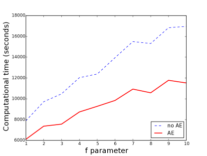
Figure 17: Test 2: Comparison of the computational time between a simulation with and without asynchronous evolution. The blue dashed line shows the results for the case without asynchronous evolution and the red solid line the same for the case with asynchronous evolution. For this test, the gain is between 33% and 40%.

7.3 Test 3 - Multiple sources in a cosmological field

This test is the standard cosmological density field test from the Cosmological Radiative Transfer Code Comparison Project (Iliev et al., 2006b). The simulation volume contains a cosmological density field of size €$0.5\,h^{-1}$ comoving Mpc. The resolution is $128^{3}$ cells. The initial temperature of the gas is $T=100$ K. Sixteen ionizing sources are placed at the location of the 16 most massive haloes in the simulation volume. Each source produces $f_{\gamma}=250$ ionizing photons per atom over a time interval $t_{s}=3$ Myr. The ionizing photon production rate of each source is calculated from

$$\dot{N}_{\gamma}=f_{\gamma}\frac{M\Omega_{\mathrm{b}}}{\Omega_{\mathrm{m}}m_{\mathrm{p}}t_{\mathrm{s}}}\,,$$ (21)

with $M$ the halo mass and $m_{\mathrm{p}}$ the mass of a proton. All sources have a black body spectrum with $T_{\mathrm{eff}}=10^{5}$ K. The cosmological parameters used are $\Omega_{\Lambda}=0.73$, $\Omega_{\mathrm{m}}=0.27$, $\Omega_{\mathrm{b}}=0.043$, $h=0.7$. The total evolution time is 0.40 Myr. For our asynchronous evolution approach we use $x_{\mbox{\scriptsize{HI}}}\leq 1\times 10^{-4}$ and $x_{\mbox{\scriptsize{HeII}}}\leq 3\times 10^{-4}$ as the criteria for equilibrium of the ionized cells.

First, we compare the thermal results between a constant time-step approach and the adaptive time-step approach. For the constant time-step case we use a time-step of $0.05$ Myr. For the adaptive time-step approach we use $f=2$. Figures 18 and 19 show our temperature results of a central slice at $t=0.05$ Myr and $0.2$ Myr, respectively.

Figure 18 shows the typical butterfly shape of the temperature distribution associated with this test. The left plot displays the result of a single time-step evolution (constant time-step approach). We see that the temperature has its local maximum at the ionization front similar to what we saw in the results for Test 1 above. The right plot shows the result of adaptive time-step approach. Here there is no pronounced thermal maximum at the ionization front and no abrupt change in the thermal structure in the ionized regions.

Figure 19 shows the late time results ($t=0.2$ Myr). The left plot shows the temperature distribution after 4 constant time-steps. We can discern multiple sharp layers corresponding to the different ionization front positions at those four time-steps. The right plot shows the result for the adaptive time-step approach. We see some thermal structures in the large ionized bubble. However, these structures do not trace previous ionization front positions. Instead, they correlate with the gas distribution in the sense that higher density regions attain higher temperatures than lower density regions.

We have also used this test problem to evaluate the performance of the adaptive time-step approach compared to the constant time-step approach. We find that converged results require a value of $\Delta t=2.5\times 10^{-4}$ Myr in case of the constant time-step approach and a value of $f=2$ in case of the adaptive time-step approach. The dots in Figure 20 show the computational time consumed by adopting different constant time-steps. The converged simulation which uses a constant time-step of $2.5\times 10^{-4}$ Myr consumed 431056 seconds (CPU time) and is indicated by a larger dot and a dashed line. The value for the simulation with an adaptive time-step ($f=2$), 97636 seconds, is indicated by the lower horizontal dashed line. Therefore we conclude that for this problem the adaptive time-step approach is a factor 4.4 more efficient than the constant time-step approach. From the figure it can also be seen that the computational time consumed by the adaptive time-step approach is equivalent to the case of a constant time-step $2.1\times 10^{-3}$ Myr.

Lastly, we compare the temperature results of three constant time-step simulations ($\Delta t=0.05,2.5\times 10^{-3}$ and $2.5\times 10^{-4}$ Myr) with those from the adaptive time-step simulation. Figure 21 shows the temperature profiles along the three different coordinate directions traversing one of the sources. The long constant time-step case ($\Delta t=0.05$ Myr, blue dotted line) produces a large scale uneven thermal distribution unrelated to the gas density. The converged case ($\Delta t=2.5\times 10^{-4}$ Myr, red dashed line) and the adaptive time-step simulation (black solid line) produce essentially the same thermal profiles. The constant time-step case with an equivalent computational time to the adaptive time-step simulation ($\Delta t=2.5\times 10^{-3}$ Myr, green dot-dashed line) produces better results than the long time-step case but still does not produce a correct thermal profile in a region approximately one-fifth of the box size centered around the source. This shows the advantage of the adaptive time-step approach over the constant time-step approach.

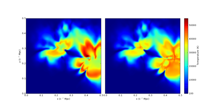
Figure 18: Test 3: Temperature structure cross section at $t=0.05$ Myr. Left panel: constant time-step ($\Delta t=5.0\times 10^{-2}$ Myr). Right panel: adaptive time-step ($f=2$).

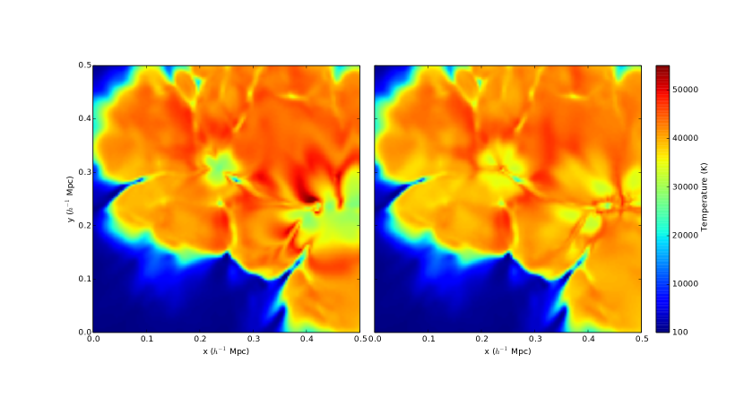
Figure 19: Test 3: Temperature structure cross section at $t=0.20$ Myr. Left panel: constant time-step ($\Delta t=5.0\times 10^{-2}$ Myr). Right panel: adaptive time-step ($f=2$).

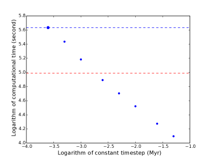
Figure 20: Test 3: A plot of computational time against different choices of constant time-steps. The 8 blue dots correspond to the $\Delta t$ values (from left to right) {$2.5\times 10^{-4}$, $5.0\times 10^{-4}$, $1.0\times 10^{-3}$, $2.5\times 10^{-3}$, $5.0\times 10^{-3}$, $1.0\times 10^{-2}$, $2.5\times 10^{-2}$, $5.0\times 10^{-2}$} Myr. The red dashed and blue dashed lines (crossing the big blue dot) show the computational time required to run the adaptive time-step model and a converged constant time-step model, respectively.

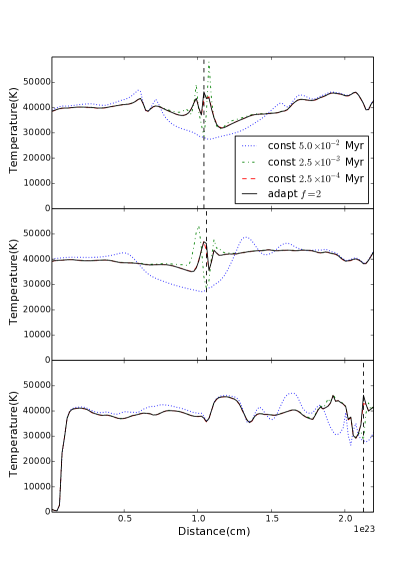
Figure 21: Test 3: Temperature structures along three perpendicular directions through one of the sixteen sources at $t=0.40$ Myr. Blue dotted line: $\Delta t=0.05$ Myr, green dot-dashed line: $\Delta t=2.5\times 10^{-3}$ Myr, red dashed line: $\Delta t=2.5\times 10^{-4}$ Myr, black solid line: adaptive time-step with $f=2$.

7.4 Test 4 - C²-Ray versus SNC

Lastly, we compare the C²-Ray results with those obtained with a different photo-ionization code, namely SNC. The base of this code is briefly described in Lundqvist & Fransson (1988), while updates were given in Lundqvist & Fransson (1991, 1996) and Mattila et al. (2010). SNC is a time-dependent photo-ionization code which includes elements from hydrogen to iron, with several of the ions being treated with multi-level atoms. It has been mainly used to calculate the time-dependent ionization and temperature of gas around supernovae and in supernova remnants, but has also been recently used in a cosmological application to study time-dependent effects of ionization by Population III stars (Rydberg et al., 2013). The code generally deals with spherically symmetric nebulae.

Time-steps in SNC are calculated for each radial shell, based on the accepted fastest changes in degrees of ionization/recombination and temperature. Normally, an accepted change is a few per cent per time-step for the ionization and about a factor of ten smaller change in temperature. A time-step also cannot be longer than the light-crossing time of a shell. Just as the new version of C²-Ray the conditions in each shell are not calculated every time-step. However, even if the selected time-step for a particular shell could formally be substantially longer than at the ionization front, the largest time step allowed for all shells is $k$ times the shortest time step; here we use $k=7$.

In terms of the atomic physics, both C²-Ray and SNC calculate all ions time-dependently. However, SNC also treats all included levels of HI, HeI and HeII time-dependently. This is however, of minor importance for cosmological applications. Of greater importance is the treatment of the diffuse emission. For this SNC uses a modified on-the-spot approximation in which recombination photons which can escape from the local environment are allowed to do so. If they can not, they are absorbed locally. However, escaping recombination photons are assumed to escape from the entire system and cannot be absorbed elsewhere.

The SNC code treats photon escape in spectral lines using escape probabilities. For spectral lines capable of ionizing HI or HeI, the probability of the photon being trapped by the continuum is also calculated. The fractions absorbed by the continuum are included in the ionization balance, and the ones scattered by lines are fed into the calculations of the level populations of the multi-level atoms of H and He. For the results discussed below, no velocity field is assumed, so the only broadening mechanisms are thermal broadening and natural line broadening.

To calculate the collisional excitation rates of H and He, SNC has since Lundqvist & Fransson (1996) been updated with the effective collision strengths of Anderson et al. (2000) and Kisielius et al. (1995) for HI and HeII, respectively. SNC also includes heating, excitation and further ionization due to fast photo-electrons, just as C²-Ray does. SNC does this by using interpolation between the calculated Spencer-Fano results of Kozma & Fransson (1998), where the inputs are the local number densities of electrons, HI and HeI.

To compare the results of C²-Ray and SNC, we have performed a 1D simulation of a spherical nebula with a particle density of $7\times 10^{-5}$ cm^-3 and consisting of He and H with a number density ratio of 0.08. The domain size is 3 Mpc, divided into 1000 cells. The value of $f$ used is 2 and for SNC the time steps are calculated according to the criteria outlined above. The initial temperature is 100 K. For the ionizing spectrum we use a power-law source with energy index 1.5. The total rate of ionizing photons is $10^{56}$ s^-1. We evolve the nebula for $10$ Myrs.

Figure 22 shows our results for the thermal and ionization evolution at $0.1,0.3,1.0,3.0,10.0$ Myr. Concentrating first on the temperature results, we see that the general shapes of the thermal profiles are similar. The temperature climbs to its maximum in the region between the source and the HeIII ionization front. The value of the peak temperature in the SNC results is some 4% higher than in C²-Ray, which is the largest difference seen between the two results.

The lower temperatures close to the source are caused by the lower column densities there. Due to these the gas close to the source encounters a larger number of low energy photons. As these are preferentially absorbed due to their higher ionization cross section, this leads to lower temperatures in the innermost parts of the ionized region. This is seen in both simulations. Outward from the peak, the temperature decreases because of the presence of substantial amounts of helium gas that have not been fully ionized and heated yet. Both sets of results show this feature. The temperature decreases rapidly at the HII region boundary and exhibits a smoothly decreasing tail. This gas outside the HII region is not ionized but heated by the high energy photons which have a high mean free path in the neutral gas. Both experiments capture the transfer of high energy photons in the neutral gas and the thermal response when these photons are gradually absorbed by the gas.

The lower two panels of Figure 22 show the evolution of $x_{\mbox{\scriptsize{HI}}}$ and $x_{\mbox{\scriptsize{HeIII}}}$ respectively. The $x_{\mbox{\scriptsize{HI}}}$ evolution of both experiments agree. Although SNC gives a slightly smaller HII region than C²-Ray, their profiles at $x_{\mbox{\scriptsize{HI}}}\geq 0.99$ coincide with each other. The agreement on the $x_{\mbox{\scriptsize{HeIII}}}$ evolution is excellent and the profiles are almost indistinguishable.

Overall, both sets of results show a high level of consistency with each other. We therefore conclude that the results of both codes agree with each other. Given the different algorithms used in the two codes, as well as their different origins, this increases the likelihood that the results are correct.

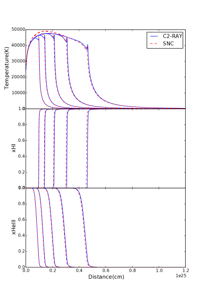
Figure 22: Test 4: Comparison of the C²-Ray and the SNC results for the temperature, $x_{\mbox{\scriptsize{HI}}}$ and $x_{\mbox{\scriptsize{HeIII}}}$ evolution. Five time instances are shown in the plots. They correspond to quasar ages of $0.1,0.3,1.0,3.0,10.0$ Myr.

8 Conclusions

Especially for photo-ionization calculations of the low density IGM, an accurate determination of the photo-heating rate is important. Since the photo-heating rate depends sensitively on the energy of the photons responsible for the photo-ionization, an accurate calculation of the photo-heating rate is more challenging than an accurate calculation of the photo-ionization rate. Specifically, the large time-step approach used by previous versions of C²-Ray provides an accurate determination of the photo-ionization rates but does not yield accurate photo-heating rates. The latter requires time-steps which temporally resolve the ionization of each cell.

We present a new version of C²-Ray which calculates the required time-step on the fly and at the same time implements two methods to reduce the computational costs associated with this. Our adaptive time-step algorithm calculates an optimal time-step by only considering the relevant cells for this calculation. These cells are identified by a fast and parallelizable ray-tracing method based on a pyramidal decomposition of the volume. To further reduce the computational cost, the code also uses asynchronous evolution which means that different cells are evolved with different time-steps. Specifically, cells which have already been ionized are evolved with much longer time-steps than the cells which still need to be ionized. The clocks of the different cells are synchronized at the end of each simulation step.

These techniques ensure that most of the computational resources are allocated to cells that potentially undergo substantial thermal evolution. The updated version of the code retains the efficient parallelization of the previous versions, using a combination of distributed and shared memory parallelization.

We have tested the new version of C²-Ray against the older version and showed that it achieves the same accuracy at a much lower computational cost. We also compare the results to another time-dependent photo-ionization code (SNC) and show that the two codes show good agreement both on the ionization fractions and the temperature.

The new version constitutes a major improvement over the previous versions. However, it is important to point out that this improvement only affects calculations of the temperature evolution. To date, all C²-Ray simulations of reionization did not consider the thermal evolution and therefore those results remain valid (e.g. Iliev et al., 2012; Datta et al., 2012; Iliev et al., 2014). Since the recombination rates only weakly depend on the temperature, the thermal state of the gas does not influence the reionization process much. Also, under the assumption of a spin temperature well above the CMB temperature, the redshifted 21cm signal does not actually depend on the gas temperature (Furlanetto et al., 2006). Thermal calculations are therefore not necessary for the later stages of reionization. The new version of C²-Ray is useful to explore the earlier phases of reionization when hard photons from x-ray sources had not yet fully raised the temperature of the IGM above the CMB temperature as well as other problems in which the temperature of the IGM is important, for example the structure of near zones around high redshift quasars.

We note that the pyramidal ray tracing scheme may have applications beyond the one presented here. It is a very efficient method of finding cells nearest to a given position which have a certain property. For example, it could be employed to find the probability distribution function of distances to edges of ionized regions, one of the methods to characterize the size distribution of ionized regions in reionization simulations (Mesinger & Furlanetto, 2007)

This paper contains a comparison of the new version of C²-Ray with the time-dependent photo-ionization code SNC. However, it would be very useful to compare a wider range of codes developed for photo-ionization calculations of the IGM in the context of a code comparison. As the hydrogen-only results of the Cosmological Radiative Transfer Comparison Project show (Iliev et al., 2006b), there can be considerable spread in the temperature results. A more detailed evaluation, including not only the temperature, but for example also the photo-heating rates, would be useful, both for the existing codes as well as for the development of new codes.

References

- Anderson et al. (2000) Anderson H., Ballance C. P., Badnell N. R., Summers H. P., 2000, J. Phys. B, 33, 1255
- Bolton et al. (2012) Bolton J. S., Becker G. D., Raskutti S., Wyithe J. S. B., Haehnelt M. G., Sargent W. L. W., 2012, MNRAS, 419, 2880
- Bolton et al. (2010) Bolton J. S., Becker G. D., Wyithe J. S. B., Haehnelt M. G., Sargent W. L. W., 2010, MNRAS, 406, 612
- Bolton & Haehnelt (2007) Bolton J. S., Haehnelt M. G., 2007, MNRAS, 374, 493
- Bolton et al. (2011) Bolton J. S., Haehnelt M. G., Warren S. J., Hewett P. C., Mortlock D. J., Venemans B. P., McMahon R. G., Simpson C., 2011, MNRAS, 416, L70
- Cantalupo & Porciani (2011) Cantalupo S., Porciani C., 2011, MNRAS, 411, 1678
- Cen et al. (2009) Cen R., McDonald P., Trac H., Loeb A., 2009, ApJ, 706, L164
- Datta et al. (2012) Datta K. K., Friedrich M. M., Mellema G., Iliev I. T., Shapiro P. R., 2012, MNRAS, 424, 762
- Fan et al. (2006) Fan X. et al., 2006, AJ, 132, 117
- Ferland et al. (2013) Ferland G. J. et al., 2013, Rev. Mexicana Astron. Astrofis., 49, 137
- Friedrich et al. (2012) Friedrich M. M., Mellema G., Iliev I. T., Shapiro P. R., 2012, MNRAS, 421, 2232
- Furlanetto et al. (2006) Furlanetto S. R., Oh S. P., Briggs F. H., 2006, Phys. Rep., 433, 181
- Graziani et al. (2013) Graziani L., Maselli A., Ciardi B., 2013, MNRAS, 431, 722
- Hui & Haiman (2003) Hui L., Haiman Z., 2003, ApJ, 596, 9
- Iliev et al. (2006a) Iliev I. T. et al., 2006a, MNRAS, 371, 1057
- Iliev et al. (2006b) Iliev I. T. et al., 2006b, MNRAS, 371, 1057
- Iliev et al. (2014) Iliev I. T., Mellema G., Ahn K., Shapiro P. R., Mao Y., Pen U.-L., 2014, MNRAS, 439, 725
- Iliev et al. (2006c) Iliev I. T., Mellema G., Pen U.-L., Merz H., Shapiro P. R., Alvarez M. A., 2006c, MNRAS, 369, 1625
- Iliev et al. (2012) Iliev I. T., Mellema G., Shapiro P. R., Pen U.-L., Mao Y., Koda J., Ahn K., 2012, MNRAS, 423, 2222
- Iliev et al. (2011) Iliev I. T., Moore B., Gottlöber S., Yepes G., Hoffman Y., Mellema G., 2011, MNRAS, 413, 2093
- Iliev et al. (2009) Iliev I. T. et al., 2009, MNRAS, 400, 1283
- Kisielius et al. (1995) Kisielius R., Berrington K. A., Norrington P. H., 1995, J. Phys. B, 28, 2459
- Kozma & Fransson (1998) Kozma C., Fransson C., 1998, ApJ, 496, 946
- Kunasz & Auer (1988) Kunasz P., Auer L. H., 1988, J. Quant. Spec. Radiat. Transf., 39, 67
- Lundqvist & Fransson (1988) Lundqvist P., Fransson C., 1988, A&A, 192, 221
- Lundqvist & Fransson (1991) Lundqvist P., Fransson C., 1991, ApJ, 380, 575
- Lundqvist & Fransson (1996) Lundqvist P., Fransson C., 1996, ApJ, 464, 924
- Mackey (2012) Mackey J., 2012, A&A, 539, A147
- Mattila et al. (2010) Mattila S., Lundqvist P., Gröningsson P., Meikle P., Stathakis R., Fransson C., Cannon R., 2010, ApJ, 717, 1140
- Mellema et al. (2006) Mellema G., Iliev I. T., Alvarez M. A., Shapiro P. R., 2006, New A, 11, 374
- Mesinger & Furlanetto (2007) Mesinger A., Furlanetto S., 2007, ApJ, 669, 663
- Mesinger & Haiman (2007) Mesinger A., Haiman Z., 2007, ApJ, 660, 923
- Norman et al. (1998) Norman M. L., Paschos P., Abel T., 1998, Mem. Soc. Astron. Italiana, 69, 455
- Paciga et al. (2013) Paciga G. et al., 2013, MNRAS, 433, 639
- Parsons et al. (2010) Parsons A. R. et al., 2010, AJ, 139, 1468
- Pawlik & Schaye (2011) Pawlik A. H., Schaye J., 2011, MNRAS, 412, 1943
- Pritchard & Furlanetto (2007) Pritchard J. R., Furlanetto S. R., 2007, MNRAS, 376, 1680
- Raičević et al. (2014) Raičević M., Pawlik A. H., Schaye J., Rahmati A., 2014, MNRAS, 437, 2816
- Raskutti et al. (2012) Raskutti S., Bolton J. S., Wyithe J. S. B., Becker G. D., 2012, MNRAS, 421, 1969
- Ricotti et al. (2002) Ricotti M., Gnedin N. Y., Shull J. M., 2002, ApJ, 575, 33
- Rydberg et al. (2013) Rydberg C.-E., Zackrisson E., Lundqvist P., Scott P., 2013, MNRAS, 429, 3658
- Schroeder et al. (2013) Schroeder J., Mesinger A., Haiman Z., 2013, MNRAS, 428, 3058
- Theuns et al. (2002) Theuns T., Schaye J., Zaroubi S., Kim T.-S., Tzanavaris P., Carswell B., 2002, ApJ, 567, L103
- Tingay et al. (2013) Tingay S. J. et al., 2013, PASA, 30, 7
- Trac & Gnedin (2011) Trac H. Y., Gnedin N. Y., 2011, Advanced Science Letters, 4, 228
- van Haarlem et al. (2013) van Haarlem M. P. et al., 2013, A&A, 556, A2
- Willott et al. (2007) Willott C. J. et al., 2007, AJ, 134, 2435