Error estimates of numerical methods for
the nonlinear Dirac equation
in the nonrelativistic limit regime

Abstract

We present several numerical methods and establish their error estimates for the discretization of the nonlinear Dirac equation in the nonrelativistic limit regime, involving a small dimensionless parameter $0<\varepsilon\ll 1$ which is inversely proportional to the speed of light. In this limit regime, the solution is highly oscillatory in time, i.e. there are propagating waves with wavelength $O(\varepsilon^{2})$ and $O(1)$ in time and space, respectively. We begin with the conservative Crank-Nicolson finite difference (CNFD) method and establish rigorously its error estimate which depends explicitly on the mesh size $h$ and time step $\tau$ as well as the small parameter $0<\varepsilon\leq 1$. Based on the error bound, in order to obtain ‘correct’ numerical solutions in the nonrelativistic limit regime, i.e. $0<\varepsilon\ll 1$, the CNFD method requests the $\varepsilon$-scalability: $\tau=O(\varepsilon^{3})$ and $h=O(\sqrt{\varepsilon})$. Then we propose and analyze two numerical methods for the discretization of the nonlinear Dirac equation by using the Fourier spectral discretization for spatial derivatives combined with the exponential wave integrator and time-splitting technique for temporal derivatives, respectively. Rigorous error bounds for the two numerical methods show that their $\varepsilon$-scalability is improved to $\tau=O(\varepsilon^{2})$ and $h=O(1)$ when $0<\varepsilon\ll 1$ compared with the CNFD method. Extensive numerical results are reported to confirm our error estimates.

35Q55, 65M70, 65N12, 65N15, 81Q05

Citation:​​​​

Bao W, Cai Y, Jia X, Yin J. . Sci China Math, 2016, 59, doi:

1 Introduction

In particle physics and/or relativistic quantum mechanics, the Dirac equation, which was derived by the British physicist Paul Dirac in 1928 [27, 28], is a relativistic wave equation for describing all spin-$1/2$ massive particles, such as electrons and positrons. It is consistent with both the principle of quantum mechanics and the theory of special relativity, and was the first theory to fully account for relativity in the context of quantum mechanics. It accounted for the fine details of the hydrogen spectrum in a completely rigorous way and provided the entailed explanation of spin as a consequence of the union of quantum mechanics and relativity – and the eventual discovery of the positron – represent one of the greatest triumphs of theoretical physics. Since the graphene was first produced in the lab in 2003 [1, 62], the Dirac equation has been extensively adopted to study theoretically the structures and/or dynamical properties of graphene and graphite as well as other two dimensional (2D) materials [1, 32, 62]. Recently, the Dirac equation has also been adopted to study the relativistic effects in molecules in super intense lasers, e.g. attosecond lasers [34, 35] and the motion of nucleons in the covariant density function theory in the relativistic framework [65, 55].

The nonlinear Dirac equation (NLDE), which was proposed in 1938 [47], is a model of self-interacting Dirac fermions in quantum field theory [36, 38, 69, 73] and is widely considered as a toy model of self-interacting spinor fields in quantum physics [69, 73]. In fact, it also appears in the Einstein-Cartan-Sciama-Kibble theory of gravity, which extends general relativity to matter with intrinsic angular momentum (spin) [46]. In the resulting field equations, the minimal coupling between the homogeneous torsion tensor and Dirac spinors generates an axial-axial, spin-spin interaction in fermionic matter, which becomes nonlinear (cubic) in the spinor field and significant only at extremely high densities. Recently, the NLDE has been adapted as a mean field model for Bose-Einstein condensates (BECs) [23, 41, 42] and/or cosmology [66]. In fact, the experimental advances in BECs and/or graphene as well as 2D materials have renewed extensively the research interests on the mathematical analysis and numerical simulations of the Dirac equation and/or the NLDE without/with electromagnetic potentials, especially the honeycomb lattice potential [2, 32, 33].

Consider the NLDE in three dimensions (3D) for describing the dynamics of spin-$1/2$ self-interacting massive Dirac fermions within external time-dependent electromagnetic potentials [27, 36, 38, 69, 73, 41, 42]

$$i\hbar\partial_{t}\Psi=\Bigl{[}-ic\hbar\sum_{j=1}^{3}\alpha_{j}\partial_{j}+mc^{2}\beta\Bigr{]}\Psi+e\Bigl{[}V(t,\mathbb{x})I_{4}-\sum_{j=1}^{3}A_{j}(t,\mathbf{x})\alpha_{j}\Bigr{]}\Psi+{\bf F}(\Psi)\Psi,\quad{\bf x}\in{\mathbb{R}}^{3},$$ (1.1)

where $i=\sqrt{-1}$, $t$ is time, ${\bf x}=(x_{1},x_{2},x_{3})^{T}\in{\mathbb{R}}^{3}$ (equivalently written as ${\bf x}=(x,y,z)^{T}$) is the spatial coordinate vector, $\partial_{k}=\frac{\partial}{\partial x_{k}}$ ($k=1,2,3$), $\Psi:=\Psi(t,{\bf x})=(\psi_{1}(t,{\bf x}),\psi_{2}(t,{\bf x}),\psi_{3}(t,{\bf x}),\psi_{4}(t,{\bf x}))^{T}\in\mathbb{C}^{4}$ is the complex-valued vector wave function of the “spinorfield”. $I_{n}$ is the $n\times n$ identity matrix for $n\in{\mathbb{N}}$, $V:=V(t,{\bf x})$ is the real-valued electrical potential and ${\bf A}:={\bf A}(t,{\bf x})=(A_{1}(t,{\bf x}),A_{2}(t,{\bf x}),A_{3}(t,{\bf x}))^{T}$ is the real-valued magnetic potential vector, and hence the electric field is given by ${\bf E}(t,{\bf x})=-\nabla V-\partial_{t}{\bf A}$ and the magnetic field is given by ${\bf B}(t,{\bf x})={\rm curl}\,{\bf A}=\nabla\times{\bf A}$. Different cubic nonlinearities have been proposed and studied for the NLDE (1.1) from different applications [36, 38, 69, 73, 41, 42]. For the simplicity of notations, here we take ${\bf F}(\Psi)=g_{1}\left(\Psi^{*}\beta\Psi\right)\beta+g_{2}|\Psi|^{2}I_{4}$ with $g_{1},g_{2}\in{\mathbb{R}}$ two constants and $\Psi^{*}=\overline{\Psi}^{T}$, while $\overline{f}$ denotes the complex conjugate of $f$, which is motivated from the so-called Soler model, e.g. $g_{2}=0$ and $g_{1}\neq 0$, in quantum field theory [36, 38, 69, 73] and BECs with a chiral confinement and/or spin-orbit coupling, e.g. $g_{1}=0$ and $g_{2}\neq 0$ [23, 41, 42]. We remark here that our numerical methods and their error estimates can be easily extended to the NLDE with other nonlinearities [73, 66, 67]. The physical constants are: $c$ for the speed of light, $m$ for the particle’s rest mass, $\hbar$ for the Planck constant and $e$ for the unit charge. In addition, the $4\times 4$ matrices $\alpha_{1}$, $\alpha_{2}$, $\alpha_{3}$ and $\beta$ are defined as

$$\alpha_{1}=\left(\begin{array}[]{cc}\mathbf{0}&\sigma_{1}\\ \sigma_{1}&\mathbf{0}\\ \end{array}\right),\qquad\alpha_{2}=\left(\begin{array}[]{cc}\mathbf{0}&\sigma_{2}\\ \sigma_{2}&\mathbf{0}\\ \end{array}\right),\qquad\alpha_{3}=\left(\begin{array}[]{cc}\mathbf{0}&\sigma_{3}\\ \sigma_{3}&\mathbf{0}\\ \end{array}\right),\qquad\beta=\left(\begin{array}[]{cc}I_{2}&\mathbf{0}\\ \mathbf{0}&-I_{2}\\ \end{array}\right),$$ (1.2)

with $\sigma_{1}$, $\sigma_{2}$, $\sigma_{3}$ (equivalently written $\sigma_{x}$, $\sigma_{y}$, $\sigma_{z}$) being the Pauli matrices defined as

$$\sigma_{1}=\left(\begin{array}[]{cc}0&1\\ 1&0\\ \end{array}\right),\qquad\sigma_{2}=\left(\begin{array}[]{cc}0&-i\\ i&0\\ \end{array}\right),\qquad\sigma_{3}=\left(\begin{array}[]{cc}1&0\\ 0&-1\\ \end{array}\right).$$ (1.3)

Similar to the Dirac equation [11], by a proper nondimensionalization (with the choice of $x_{s}$, $t_{s}=\frac{mx_{s}^{2}}{\hbar}$, $A_{s}=\frac{mv^{2}}{e}$ and $\psi_{s}=x_{s}^{-3/2}$ as the dimensionless length unit, time unit, potential unit and spinor field unit, respectively) and dimension reduction [11], we can obtain the dimensionless NLDE in $d$-dimensions ($d=3,2,1$)

$$i\partial_{t}\Psi=\Bigl{[}-\frac{i}{\varepsilon}\sum_{j=1}^{d}\alpha_{j}\partial_{j}+\frac{1}{\varepsilon^{2}}\beta\Bigr{]}\Psi+\Bigl{[}V(t,{\bf x})I_{4}-\sum_{j=1}^{d}A_{j}(t,{\bf x})\alpha_{j}\Bigr{]}\Psi+{\bf F}(\Psi)\Psi,\quad{\bf x}\in{\mathbb{R}}^{d},$$ (1.4)

where $\varepsilon$ is a dimensionless parameter inversely proportional to the speed of light given by

$$0<\varepsilon:=\frac{x_{s}}{t_{s}\,c}=\frac{v}{c}\leq 1,$$ (1.5)

with $v=\frac{x_{s}}{t_{s}}$ the wave speed, and

$${\bf F}(\Psi)=\lambda_{1}\left(\Psi^{*}\beta\Psi\right)\beta+\lambda_{2}|\Psi|^{2}I_{4},\qquad\Psi\in{\mathbb{C}}^{4},$$ (1.6)

with $\lambda_{1}=\frac{g_{1}}{mv^{2}x_{s}^{3}}\in{\mathbb{R}}$ and $\lambda_{2}=\frac{g_{2}}{mv^{2}x_{s}^{3}}\in{\mathbb{R}}$ two dimensionless constants for the interaction strength.

For the dynamics, the initial condition is given as

$$\Psi(t=0,{\bf x})=\Psi_{0}({\bf x}),\qquad{\bf x}\in\mathbb{R}^{d}.$$

The NLDE (1.4) is dispersive and time symmetric [79]. Introducing the position density $\rho_{j}$ for the $j$-component ($j=1,2,3,4$), the total density $\rho$ as well as the current density ${\bf J}(t,{\bf x})=(J_{1}(t,{\bf x}),J_{2}(t,{\bf x})$, $J_{3}(t,{\bf x}))^{T}$

$$\rho(t,{\bf x})=\sum_{j=1}^{4}\rho_{j}(t,{\bf x})=\Psi^{*}\Psi,\ \ \rho_{j}(t,{\bf x})=|\psi_{j}(t,{\bf x})|^{2},\quad 1\leq j\leq 4;\ \ J_{l}(t,{\bf x})=\frac{1}{\varepsilon}\Psi^{*}\alpha_{l}\Psi,\quad l=1,2,3,$$ (1.7)

then the following conservation law can be obtained from the NLDE (1.4)

$$\partial_{t}\rho(t,{\bf x})+\nabla\cdot{\bf J}(t,{\bf x})=0,\qquad{\bf x}\in{\mathbb{R}}^{d},\quad t>0.$$ (1.8)

Thus the NLDE (1.4) conserves the total mass as

$$\|\Psi(t,\cdot)\|^{2}:=\int_{{\mathbb{R}}^{d}}|\Psi(t,{\bf x})|^{2}\,d{\bf x}=\int_{{\mathbb{R}}^{d}}\sum_{j=1}^{4}|\psi_{j}(t,{\bf x})|^{2}\,d{\bf x}\equiv\|\Psi(0,\cdot)\|^{2}=\|\Psi_{0}\|^{2},\qquad t\geq 0.$$ (1.9)

If the electric potential $V$ is perturbed by a constant, e.g. $V(t,{\bf x})\to V(t,{\bf x})+V^{0}$ with $V^{0}$ being a real constant, then the solution $\Psi(t,{\bf x})\to e^{-iV^{0}t}\Psi(t,{\bf x})$ which implies the density of each component $\rho_{j}$ ($j=1,2,3,4$) and the total density $\rho$ unchanged. When $d=1$, if the magnetic potential $A_{1}$ is perturbed by a constant, e.g. $A_{1}(t,{\bf x})\to A_{1}(t,{\bf x})+A_{1}^{0}$ with $A_{1}^{0}$ being a real constant, then the solution $\Psi(t,{\bf x})\to e^{iA_{1}^{0}t\alpha_{1}}\Psi(t,{\bf x})$ which implies the total density $\rho$ unchanged; but this property is not valid when $d=2,3$. These properties are usually called as time transverse invariant. In addition, when the electromagnetic potentials are time-independent, i.e. $V(t,{\bf x})=V({\bf x})$ and $A_{j}(t,{\bf x})=A_{j}({\bf x})$ for $j=1,2,3$, the following energy functional is also conserved

$$E(t) := \int_{\mathbb{R}^{d}}\left[-\frac{i}{\varepsilon}\sum_{j=1}^{d}\Psi^{*}\alpha_{j}\partial_{j}\Psi+\frac{1}{\varepsilon^{2}}\Psi^{*}\beta\Psi+V({\bf x})|\Psi|^{2}+G(\Psi)-\sum_{j=1}^{d}A_{j}({\bf x})\Psi^{*}\alpha_{j}\Psi\right]d{\bf x}$$ (1.10)

$$\equiv E(0),\qquad t\geq 0,$$

where

$$G(\Psi)=\frac{\lambda_{1}}{2}\left(\Psi^{*}\beta\Psi\right)^{2}+\frac{\lambda_{2}}{2}|\Psi|^{4},\qquad\Psi\in{\mathbb{C}}^{4}.$$ (1.11)

Furthermore, if the external electromagnetic potentials are constants, i.e. $V(t,{\bf x})\equiv V^{0}$ and $A_{j}(t,{\bf x})\equiv A_{j}^{0}$ for $j=1,2,3$, the NLDE (1.4) admits the plane wave solution as $\Psi(t,{\bf x})={\bf B}\,e^{i({\bf k}\cdot{\bf x}-\omega t)}$, where the time frequency $\omega$, amplitude vector ${\bf B}\in{\mathbb{R}}^{4}$ and spatial wave number ${\bf k}=(k_{1},\ldots,k_{d})^{T}\in{\mathbb{R}}^{d}$ satisfy

$$\omega{\bf B}=\left[\sum_{j=1}^{d}\left(\frac{k_{j}}{\varepsilon}-A_{j}^{0}\right)\alpha_{j}+\frac{1}{\varepsilon^{2}}\beta+V^{0}I_{4}+\lambda_{1}\left({\bf B}^{*}\beta{\bf B}\right)\beta+\lambda_{2}|{\bf B}|^{2}I_{4}\right]{\bf B},$$ (1.12)

which immediately implies the dispersion relation of the NLDE (1.4) as

$$\omega:=\omega({\bf k},{\bf B})=V^{0}+\lambda_{2}|{\bf B}|^{2}\pm\frac{1}{\varepsilon^{2}}\sqrt{\left[1+\varepsilon^{2}\lambda_{1}\left({\bf B}^{*}\beta{\bf B}\right)\right]^{2}+\varepsilon^{2}\left|{\bf k}-\varepsilon{\bf A}^{0}\right|^{2}}=O\left(\frac{1}{\varepsilon^{2}}\right),\quad{\bf k}\in{\mathbb{R}}^{d}.$$ (1.13)

Again, similar to the Dirac equation [11], in several applications in one dimension (1D) and two dimensions (2D), the NLDE (1.4) can be simplified to the following NLDE in $d$-dimensions ($d=1,2$) with $\Phi:=\Phi(t,{\bf x})=(\phi_{1}(t,{\bf x}),\phi_{2}(t,{\bf x}))^{T}\in{\mathbb{C}}^{2}$ [36, 38, 69]

$$i\partial_{t}\Phi=\Bigl{[}-\frac{i}{\varepsilon}\sum_{j=1}^{d}\sigma_{j}\partial_{j}+\frac{1}{\varepsilon^{2}}\sigma_{3}\Bigr{]}\Phi+\Bigl{[}V(t,{\bf x})I_{2}-\sum_{j=1}^{d}A_{j}(t,{\bf x})\sigma_{j}\Bigr{]}\Phi+{\bf F}(\Phi)\Phi,\quad{\bf x}\in{\mathbb{R}}^{d},$$ (1.14)

where

$${\bf F}(\Phi)=\lambda_{1}\left(\Phi^{*}\sigma_{3}\Phi\right)\sigma_{3}+\lambda_{2}|\Phi|^{2}I_{2},\qquad\Phi\in{\mathbb{C}}^{2},$$ (1.15)

with $\lambda_{1}\in{\mathbb{R}}$ and $\lambda_{2}\in{\mathbb{R}}$ two dimensionless constants for the interaction strength. Again, the initial condition for dynamics is given as

$$\Phi(t=0,{\bf x})=\Phi_{0}({\bf x}),\qquad{\bf x}\in{\mathbb{R}}^{d}.$$ (1.16)

The NLDE (1.14) is dispersive and time symmetric. By introducing the position density $\rho_{j}$ for the $j$-th component ($j=1,2$), the total density $\rho$ as well as the current density ${\bf J}(t,{\bf x})=(J_{1}(t,{\bf x}),J_{2}(t,{\bf x}))^{T}$

$$\rho(t,{\bf x})=\sum_{j=1}^{2}\rho_{j}(t,{\bf x})=\Phi^{\ast}\Phi,\quad\rho_{j}(t,{\bf x})=|\phi_{j}(t,{\bf x})|^{2},\quad J_{j}(t,{\bf x})=\frac{1}{\varepsilon}\Phi^{*}\sigma_{j}\Phi,\quad j=1,2,$$ (1.17)

the conservation law (1.8) is also satisfied [21]. In addition, the NLDE (1.14) conserves the total mass as

$$\|\Phi(t,\cdot)\|^{2}:=\int_{{\mathbb{R}}^{d}}|\Phi(t,{\bf x})|^{2}\,d{\bf x}=\int_{{\mathbb{R}}^{d}}\sum_{j=1}^{2}|\phi_{j}(t,{\bf x})|^{2}\,d{\bf x}\equiv\|\Phi(0,\cdot)\|^{2}=\|\Phi_{0}\|^{2},\qquad t\geq 0.$$ (1.18)

Again, if the electric potential $V$ is perturbed by a constant, e.g. $V(t,{\bf x})\to V(t,{\bf x})+V^{0}$ with $V^{0}$ being a real constant, the solution $\Phi(t,{\bf x})\to e^{-iV^{0}t}\Phi(t,{\bf x})$ which implies the density of each component $\rho_{j}$ ($j=1,2$) and the total density $\rho$ unchanged. When $d=1$, if the magnetic potential $A_{1}$ is perturbed by a constant, e.g. $A_{1}(t,{\bf x})\to A_{1}(t,{\bf x})+A_{1}^{0}$ with $A_{1}^{0}$ being a real constant, the solution $\Phi(t,{\bf x})\to e^{iA_{1}^{0}t\sigma_{1}}\Phi(t,{\bf x})$ implying the total density $\rho$ unchanged; but this property is not valid when $d=2$. When the electromagnetic potentials are time-independent, i.e. $V(t,{\bf x})=V({\bf x})$ and $A_{j}(t,{\bf x})=A_{j}({\bf x})$ for $j=1,2$, the following energy functional is also conserved

$$E(t) := \int_{\mathbb{R}^{d}}\left(-\frac{i}{\varepsilon}\sum_{j=1}^{d}\Phi^{*}\sigma_{j}\partial_{j}\Phi+\frac{1}{\varepsilon^{2}}\Phi^{*}\sigma_{3}\Phi+V({\bf x})|\Phi|^{2}-\sum_{j=1}^{d}A_{j}({\bf x})\Phi^{*}\sigma_{j}\Phi+G(\Phi)\right)d{\bf x}$$ (1.19)

$$\equiv E(0),\qquad t\geq 0,$$

where

$$G(\Phi)=\frac{\lambda_{1}}{2}\left(\Phi^{*}\sigma_{3}\Phi\right)^{2}+\frac{\lambda_{2}}{2}|\Phi|^{4},\qquad\Phi\in{\mathbb{C}}^{2}.$$ (1.20)

Furthermore, if the external electromagnetic potentials are constants, i.e. $V(t,{\bf x})\equiv V^{0}$ and $A_{j}(t,{\bf x})\equiv A_{j}^{0}$ for $j=1,2$, the NLDE (1.14) admits the plane wave solution as $\Phi(t,{\bf x})={\bf B}\,e^{i({\bf k}\cdot{\bf x}-\omega t)}$, where the time frequency $\omega$, amplitude vector ${\bf B}\in{\mathbb{R}}^{2}$ and spatial wave number ${\bf k}=(k_{1},\ldots,k_{d})^{T}\in{\mathbb{R}}^{d}$ satisfy

$$\omega{\bf B}=\Bigl{[}\ \sum_{j=1}^{d}\left(\frac{k_{j}}{\varepsilon}-A_{j}^{0}\right)\sigma_{j}+\frac{1}{\varepsilon^{2}}\sigma_{3}+V^{0}I_{2}+\lambda_{1}\left({\bf B}^{*}\sigma_{3}{\bf B}\right)\sigma_{3}+\lambda_{2}|{\bf B}|^{2}I_{2}\Bigr{]}{\bf B},$$ (1.21)

which immediately implies the dispersion relation of the NLDE (1.14) as

$$\omega:=\omega({\bf k},{\bf B})=V^{0}+\lambda_{2}|{\bf B}|^{2}\pm\frac{1}{\varepsilon^{2}}\sqrt{\left[1+\varepsilon^{2}\lambda_{1}\left({\bf B}^{*}\sigma_{3}{\bf B}\right)\right]^{2}+\varepsilon^{2}\left|{\bf k}-\varepsilon{\bf A}^{0}\right|^{2}}=O\left(\frac{1}{\varepsilon^{2}}\right),\quad{\bf k}\in{\mathbb{R}}^{d}.$$ (1.22)

For the NLDE (1.4) (or (1.14)) with $\varepsilon=1$, i.e. $O(1)$-speed of light regime, there are extensive analytical and numerical results in the literatures. For the existence and multiplicity of bound states and/or standing wave solutions, we refer to [6, 7, 18, 22, 29, 30, 31, 52] and references therein. Particularly, when $d=1$, $\varepsilon=1$, $V(t,x)\equiv 0$ and $A_{1}(t,x)\equiv 0$ in (1.14) and $\lambda_{1}=-1$ and $\lambda_{2}=0$ in (1.15), the NLDE (1.14) admits soliton solutions which was given explicitly in [25, 38, 43, 53, 58, 64, 71, 72]. For the numerical methods and comparison such as the finite difference time domain (FDTD) methods [21, 45, 63], time-splitting Fourier spectral (TSFP) methods [17, 20, 26, 49] and Runge-Kutta discontinuous Galerkin methods [76, 79], we refer to [17, 20, 21, 26, 45, 48, 49, 63] and references therein. However, for the NLDE (1.4) (or (1.14)) with $0<\varepsilon\ll 1$, i.e. nonrelativistic limit regime (or the scaled speed of light goes to infinity), the analysis and efficient computation of the NLDE (1.4) (or (1.14)) are mathematically rather complicated issues. The main difficulty is due to that the solution is highly oscillatory in time and the corresponding energy functionals (1.10) and (1.19) are indefinite [19, 31] and become unbounded when $\varepsilon\to 0$. For the Dirac equation, i.e. ${\bf F}(\Psi)\equiv 0$ in (1.6) (or ${\bf F}(\Phi)\equiv 0$ in (1.15)), there are extensive mathematical analysis of the (semi)-nonrelativistic limits [50, 19, 40, 57, 78]. For the NLDE (1.4) (or (1.14)), similar analysis of the nonrelativistic limits has been done in [37, 61]. These rigorous analytical results show that the solution propagates waves with wavelength $O(\varepsilon^{2})$ and $O(1)$ in time and space, respectively, when $0<\varepsilon\ll 1$. In fact, the oscillatory structure of the solution of the NLDE (1.4) (or (1.14)) when $0<\varepsilon\ll 1$ can be formally observed from its dispersion relation (1.13) (or (1.22)). To illustrate this further, Figure 1 shows the solution of the NLDE (1.14) with $d=1$, $V(t,x)=\frac{1-x}{1+x^{2}}$, $A_{1}(t,x)=\frac{(1+x)^{2}}{1+x^{2}}$, $\lambda_{1}=-1$, $\lambda_{2}=0$ and $\Phi_{0}(x)=\left(\exp(-x^{2}/2),\exp(-(x-1)^{2}/2)\right)^{T}$ for different $\varepsilon$.

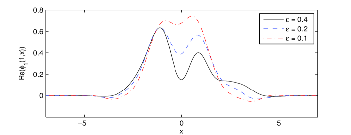
Figure 1: The solution $\phi_{1}(t=1,x)$ and $\phi_{1}(t,x=0)$ of the NLDE (1.14) with $d=1$ for different $\varepsilon$. ${\rm Re}(f)$ denotes the real part of $f$.

The highly oscillatory nature of the solution of the NLDE (1.4) (or (1.14)) causes severe numerical burdens in practical computation, making the numerical approximation of the NLDE (1.4) (or (1.14)) extremely challenging and costly in the nonrelativistic regime $0<\varepsilon\ll 1$. Recently, we compared the spatial/temporal resolution in term of $\varepsilon$ and established rigorous error estimates of the FDTD methods, TSFP methods for the Dirac equation in the nonrelativistic limit regime [11], and proposed a new uniformly accurate multiscale time integrator pseudospectral method [12]. To our knowledge, so far there are few results on the numerics of the NLDE in the nonrelativistic limit regime. The aim of this paper is to study the efficiency of the Crank-Nicolson finite difference (CNFD) and TSFP methods applied to the NLDE in the nonrelativistic limit regime, to propose the exponential wave integrator Fourier pseudospectral (EWI-FP) method and to compare their resolution capacities in this regime. We start with the detailed analysis on the convergence of the CNFD method by paying particular attention to how the error bound depends explicitly on the small parameter $\varepsilon$ in addition to the mesh size $h$ and time step $\tau$. Based on the estimate, in order to obtain ‘correct’ numerical approximations when $0<\varepsilon\ll 1$, the meshing strategy requirement ($\varepsilon$-scalability) for the CNFD (and FDTD) is: $h=O(\sqrt{\varepsilon})$ and $\tau=O(\varepsilon^{3})$, which suggests that the CNFD (and FDTD) is computationally expensive for the NLDE (1.4) (or (1.14)) as $0<\varepsilon\ll 1$. To relax the $\varepsilon$-scalability, we then propose the EWI-FP method and compare it with the TSFP method, whose $\varepsilon$-scalability are optimal for both time and space in view of the inherent oscillatory nature. The key ideas of the EWI-FP are: (i) to apply the Fourier pseudospectral discretization for spatial derivatives; and (ii) to adopt the exponential wave integrator (EWI), which was well demonstrated in the literatures that it has favorable properties compared to standard time integrators for oscillatory differential equations [39, 44], for integrating the ordinary differential equations (ODEs) in phase space [39, 44]. Rigorous error estimates show that the $\varepsilon$-scalability of the EWI-FP method is $h=O(1)$, and $\tau=O(\varepsilon^{2})$ for the NLDE with external electromagnetic potentials, meanwhile, the $\varepsilon$-scalability of the TSFP method is $h=O(1)$ and $\tau=O(\varepsilon^{2})$. Thus, the EWI-FP and TSFP offer compelling advantages over CNFD (and FDTD) for the NLDE in temporal and spatial resolution when $0<\varepsilon\ll 1$. In particular, under suitable choices of the time step, the error estimates of TSFP are much better than EWI-FP, which suggests that TSFP performs best in the nonrelativistic limit regime.

The rest of this paper is organized as follows. In Section 2, the CNFD method is reviewed and its convergence is analyzed in the nonrelativistic limit regime. In Section 3, an EWI-FP method is proposed and analyzed rigorously. In Section 4, a TSFP method is reviewed and analyzed rigorously. In Section 5, numerical comparison results are reported. Finally, some concluding remarks are drawn in Section 6. The mathematical proofs of the error estimates are given in the Appendices. Throughout the paper, we adopt the standard notations of Sobolev spaces, use the notation $p\lesssim q$ to represent that there exists a generic constant $C>0$ which is independent of $h$, $\tau$ and $\varepsilon$ such that $|p|\leq C\,q$.

2 The Crank-Nicolson finite difference (CNFD) method

In this section, we apply the CNFD method to the NLDE (1.14) (or (1.4)) with external electromagnetic field and analyze its conservation law and convergence in the nonrelativistic limit regime. For simplicity of notations, we shall only present the numerical method and its analysis for (1.14) in 1D. Generalization to (1.4) and/or higher dimensions is straightforward and results remain valid without modifications. Similar to most works in the literatures for the analysis and computation of the NLDE (cf. [3, 5, 38, 48, 76, 79] and references therein), in practical computation, we truncate the whole space problem onto an interval $\Omega=(a,b)$ with periodic boundary conditions, which is large enough such that the truncation error is negligible. In 1D, the NLDE (1.14) with periodic boundary conditions collapses to

$$i\partial_{t}\Phi=\left[-\frac{i}{\varepsilon}\sigma_{1}\partial_{x}+\frac{1}{\varepsilon^{2}}\sigma_{3}\right]\Phi+\left[V(t,x)I_{2}-A_{1}(t,x)\sigma_{1}+{\bf F}(\Phi)\right]\Phi,\qquad x\in\Omega,\quad t>0,$$ (2.1)

$$\Phi(t,a)=\Phi(t,b),\quad\partial_{x}\Phi(t,a)=\partial_{x}\Phi(t,b),\quad t\geq 0,\qquad\Phi(0,x)=\Phi_{0}(x),\quad x\in\overline{\Omega},$$ (2.2)

where $\Phi:=\Phi(t,x)\in{\mathbb{C}}^{2}$, $\Phi_{0}(a)=\Phi_{0}(b)$, $\Phi_{0}^{\prime}(a)=\Phi_{0}^{\prime}(b)$ and ${\bf F}(\Phi)$ is given in (1.15).

2.1 The CNFD method

Choose mesh size $h:=\Delta x=\frac{b-a}{M}$ with $M$ being a positive integer, time step $\tau:=\Delta t>0$ and denote the grid points and time steps as:

$$x_{j}:=a+jh,\quad j=0,1,\ldots,M;\qquad t_{n}:=n\tau,\quad n=0,1,2,\ldots.$$

Denote $X_{M}=\{{U}=(U_{0},U_{1},...,U_{M})^{T}\ |\ U_{j}\in{\mathbb{C}}^{2},j=0,1,\ldots,M,\ U_{0}=U_{M}\}$ and we always use $U_{-1}=U_{M-1}$ if it is involved. The standard $l^{2}$-norm in $X_{M}$ is given as

$$\|{U}\|^{2}_{l^{2}}=h\sum^{M-1}_{j=0}|U_{j}|^{2},\qquad{U}\in X_{M}.$$ (2.3)

Let $\Phi_{j}^{n}$ be the numerical approximation of $\Phi(t_{n},x_{j})$ and $V_{j}^{n}=V(t_{n},x_{j})$, $V_{j}^{n+1/2}=V(t_{n}+\tau/2,x_{j})$, $A_{1,j}^{n}=A_{1}(t_{n},x_{j})$, $A_{1,j}^{n+1/2}=A_{1}(t_{n}+\tau/2,x_{j})$, ${\bf F}_{j}^{n}={\bf F}(\Phi_{j}^{n})$ and ${\bf F}_{j}^{n+1/2}=\frac{1}{2}\left[{\bf F}(\Phi_{j}^{n})+{\bf F}(\Phi_{j}^{n+1})\right]$ for $0\leq j\leq M$ and $n\geq 0$. Denote $\Phi^{n}=\left(\Phi_{0}^{n},\Phi_{1}^{n},\ldots,\Phi_{M}^{n}\right)^{T}\in X_{M}$ as the solution vector at $t=t_{n}$. Introduce the finite difference discretization operators for $j=0,1,\ldots,M-1$ and $n\geq 0$ as:

$$\delta_{t}^{+}\Phi_{j}^{n}=\frac{\Phi_{j}^{n+1}-\Phi_{j}^{n}}{\tau},\qquad\delta_{t}\Phi_{j}^{n}=\frac{\Phi_{j}^{n+1}-\Phi_{j}^{n-1}}{2\tau},\qquad\delta_{x}\Phi_{j}^{n}=\frac{\Phi_{j+1}^{n}-\Phi_{j-1}^{n}}{2h},\qquad\Phi_{j}^{n+\frac{1}{2}}=\frac{\Phi_{j}^{n+1}+\Phi_{j}^{n}}{2}.$$

Here we consider the CNFD method to discretize the NLDE (2.1):

$$i\delta_{t}^{+}\Phi_{j}^{n}=\left[-\frac{i}{\varepsilon}\sigma_{1}\delta_{x}+\frac{1}{\varepsilon^{2}}\sigma_{3}+V_{j}^{n+1/2}I_{2}-A_{1,j}^{n+1/2}\sigma_{1}+{\bf F}^{n+1/2}_{j}\right]\Phi_{j}^{n+1/2},\quad 0\leq j\leq M-1,\quad n\geq 0.$$ (2.4)

The initial and boundary conditions in (2.2) are discretized as:

$$\Phi_{M}^{n+1}=\Phi_{0}^{n+1},\quad\Phi_{-1}^{n+1}=\Phi_{M-1}^{n+1},\quad n\geq 0,\qquad\Phi_{j}^{0}=\Phi_{0}(x_{j}),\quad j=0,1,...,M.$$ (2.5)

2.2 Conservation law and error estimates

Let $0<T<T^{*}$ with $T^{*}$ being the maximal existence time of the solution, and denote $\Omega_{T}=[0,T]\times\Omega$. We assume the electromagnetic potentials $V\in C(\overline{\Omega}_{T})$ and $A_{1}\in C(\overline{\Omega}_{T})$ and denote

$$(A)\hskip 113.81102ptV_{\rm max}:=\max_{(t,x)\in\overline{\Omega}_{T}}|V(t,x)|,\qquad A_{1,\rm max}:=\max_{(t,x)\in\overline{\Omega}_{T}}|A_{1}(t,x)|.\hskip 142.26378pt$$

For the CNFD method (2.4), similar to the mass and energy conservation of the Dirac equation [11], we have the following conservative properties, of which the proof is omitted here for brevity.

Lemma 2.1.

The CNFD method (2.4) conserves the mass in the discretized level, i.e.

$$\|\Phi^{n}\|_{l^{2}}^{2}:=h\sum_{j=0}^{M-1}|\Phi_{j}^{n}|^{2}\equiv h\sum_{j=0}^{M-1}|\Phi_{j}^{0}|^{2}=\|\Phi^{0}\|_{l^{2}}^{2}=h\sum_{j=0}^{M-1}|\Phi_{0}(x_{j})|^{2},\qquad n\geq 0.$$ (2.6)

Furthermore, if $V(t,x)=V(x)$ and $A_{1}(t,x)=A_{1}(x)$ are time independent, the CNFD method (2.4) conserves the energy as well

$$E_{h}^{n} = h\sum\limits_{j=0}^{M-1}\left[-\frac{i}{\varepsilon}(\Phi_{j}^{n})^{*}\sigma_{1}\delta_{x}\Phi_{j}^{n}+\frac{1}{\varepsilon^{2}}(\Phi_{j}^{n})^{*}\sigma_{3}\Phi_{j}^{n}+V(x_{j})|\Phi_{j}^{n}|^{2}-A_{1}(x_{j})(\Phi_{j}^{n})^{*}\sigma_{1}\Phi_{j}^{n}+G(\Phi_{j}^{n})\right]$$ (2.7)

$$\equiv E_{h}^{0},\qquad n\geq 0,$$

where $G(\Phi)$ is given in (1.20).

Next, we consider the error analysis of the CNFD (2.4). Motivated by the analytical results of the NLDE, we assume that the exact solution of (2.1) satisfies $\Phi\in C^{3}([0,T];(L^{\infty}(\Omega))^{2})\cap C^{2}([0,T];(W_{p}^{1,\infty}(\Omega))^{2})\cap C^{1}([0,T];(W_{p}^{2,\infty}(\Omega))^{2})\cap C([0,T];(W_{p}^{3,\infty}(\Omega))^{2})$ and

$$(B)\hskip 85.35826pt\left\|\frac{\partial^{r+s}}{\partial t^{r}\partial x^{s}}\Phi\right\|_{L^{\infty}([0,T];(L^{\infty}(\Omega))^{2})}\lesssim\frac{1}{\varepsilon^{2r}},\quad 0\leq r\leq 3,\ 0\leq r+s\leq 3,\quad 0<\varepsilon\leq 1,\hskip 113.81102pt$$

where $W_{p}^{m,\infty}(\Omega)=\{u\ |\ u\in W^{m,\infty}(\Omega),\ \partial_{x}^{l}u(a)=\partial_{x}^{l}u(b),\ l=0,\ldots,m-1\}$ for $m\geq 1$ and here the boundary values are understood in the trace sense. In the subsequent discussion, we will omit $\Omega$ when referring to the space norm taken on $\Omega$. We denote

$$M_{0}:=\max_{0\leq t\leq T}\|\Phi(t,x)\|_{L^{\infty}}\lesssim 1.$$ (2.8)

Define the grid error function ${\bf e}^{n}=({\bf e}_{0}^{n},{\bf e}_{1}^{n},\ldots,{\bf e}_{M}^{n})^{T}\in X_{M}$ as:

$${\bf e}_{j}^{n}=\Phi(t_{n},x_{j})-\Phi_{j}^{n},\qquad j=0,1,\ldots,M,\quad n\geq 0,$$ (2.9)

with $\Phi_{j}^{n}$ being the approximations obtained from the CNFD method.

For the CNFD (2.4), we can establish the error bound (see its proof in Appendix A).

Theorem 2.2.

Assume $0<\tau\lesssim\varepsilon^{3}h^{\frac{1}{4}}$, under the assumptions $(A)$ and $(B)$, there exist constants $h_{0}>0$ and $\tau_{0}>0$ sufficiently small and independent of $\varepsilon$, such that for any $0<\varepsilon\leq 1$, when $0<h\leq h_{0}$ and $0<\tau\leq\tau_{0}$ satisfying $0<h\lesssim\varepsilon^{\frac{2}{3}}$, we have the following error estimate for the CNFD method (2.4) with (2.5)

$$\|{\bf e}^{n}\|_{l^{2}}\lesssim\frac{h^{2}}{\varepsilon}+\frac{\tau^{2}}{\varepsilon^{6}},\qquad\|\Phi^{n}\|_{l^{\infty}}\leq 1+M_{0},\qquad 0\leq n\leq\frac{T}{\tau}.$$ (2.10)

Remark 2.3.

The above Theorem is still valid in higher dimensions provided that the conditions $0<\tau\lesssim\varepsilon^{3}h^{\frac{1}{4}}$ and $0<h\lesssim\varepsilon^{\frac{2}{3}}$ are replaced by $0<\tau\lesssim\varepsilon^{3}h^{C_{d}}$ and $0<h\lesssim\varepsilon^{\frac{1}{2(1-C_{d})}}$, respectively, with $C_{d}=\frac{d}{4}$ for $d=1,2,3$.

Remark 2.4.

Similar to the Dirac equation, we can easily extend other finite difference time domain (FDTD) methods including the leap-frop finite difference (LFFD) and semi-implicit finite difference (SIFD) [11, 51] to the NLDE, and the error bounds are the same as those in Theorem 2.2.

Based on Theorem 2.2 and Remark 2.4, the CNFD method (and FDTD methods) has the following temporal/spatial resolution capacity for the NLDE in the nonrelativistic limit regime. In fact, given an accuracy bound $\delta_{0}>0$, the $\varepsilon$-scalability of the CNFD method is:

$$\tau=O\left(\varepsilon^{3}\sqrt{\delta_{0}}\right)=O(\varepsilon^{3}),\qquad h=O\left(\sqrt{\delta_{0}\varepsilon}\right)=O\left(\sqrt{\varepsilon}\right),\qquad 0<\varepsilon\ll 1.$$

3 An EWI-FP method and its analysis

In this section, we propose an EWI-FP method to solve the NLDE (2.1) and establish its error bound.

3.1 The EWI-FP method

Denote $\mu_{l}=\frac{2l\pi}{b-a}$ for $l\in{\mathbb{Z}}$ and

$$Y_{M}=Z_{M}\times Z_{M},\quad Z_{M}={\rm span}\left\{\phi_{l}(x)=e^{i\mu_{l}(x-a)},\ l=-\frac{M}{2},-\frac{M}{2}+1,\ldots,\frac{M}{2}-1\right\}.$$

Let $[C_{p}(\overline{\Omega})]^{2}$ be the function space consisting of all periodic vector function $U(x):\ \overline{\Omega}=[a,b]\to{\mathbb{C}}^{2}$. For any $U(x)\in[C_{p}(\overline{\Omega})]^{2}$ and $U\in X_{M}$, define $P_{M}:\ [L^{2}(\Omega)]^{2}\rightarrow Y_{M}$ as the standard projection operator [68], $I_{M}:\ [C_{p}(\overline{\Omega})]^{2}\rightarrow Y_{M}$ and $I_{M}:X_{M}\rightarrow Y_{M}$ as the standard interpolation operator, i.e.

$$(P_{M}U)(x)=\sum_{l=-M/2}^{M/2-1}\widehat{U}_{l}\,e^{i\mu_{l}(x-a)},\quad(I_{M}U)(x)=\sum_{l=-M/2}^{M/2-1}\widetilde{U}_{l}\,e^{i\mu_{l}(x-a)},\qquad a\leq x\leq b,$$

with

$$\widehat{U}_{l}=\frac{1}{b-a}\int_{a}^{b}U(x)\,e^{-i\mu_{l}(x-a)}\,dx,\quad\widetilde{U}_{l}=\frac{1}{M}\sum_{j=0}^{M-1}U_{j}\,e^{-2ijl\pi/M},\quad l=-\frac{M}{2},\ldots,\frac{M}{2}-1,$$ (3.1)

where $U_{j}=U(x_{j})$ when $U$ is a function.

The Fourier spectral discretization for the NLDE (2.1) is as follows:

Find $\Phi_{M}:=\Phi_{M}(t,x)\in Y_{M}$, i.e.

$$\Phi_{M}(t,x)=\sum^{M/2-1}_{l=-M/2}\widehat{(\Phi_{M})}_{l}(t)\,e^{i\mu_{l}(x-a)},\qquad a\leq x\leq b,\qquad t\geq 0,$$ (3.2)

such that

$$i\partial_{t}\Phi_{M}=\left[-\frac{i}{\varepsilon}\sigma_{1}\partial_{x}+\frac{1}{\varepsilon^{2}}\sigma_{3}\right]\Phi_{M}+P_{M}\left[\left(V(t,x)I_{2}-A_{1}(t,x)\sigma_{1}+{\bf F}(\Phi_{M})\right)\Phi_{M}\right],\ \ a<x<b,\ \ t>0.\$$ (3.3)

Substituting (3.2) into (3.3), noticing the orthogonality of $\phi_{l}(x)$, we get

$$i\,\frac{d}{dt}\widehat{(\Phi_{M})}_{l}(t)=\left[\frac{\mu_{l}}{\varepsilon}\sigma_{1}+\frac{1}{\varepsilon^{2}}\sigma_{3}\right]\widehat{(\Phi_{M})}_{l}(t)+\widehat{{\bf G}(\Phi_{M})}_{l}(t),\quad t>0,\quad l=-\frac{M}{2},-\frac{M}{2}+1,\ldots,\frac{M}{2}-1,$$ (3.4)

where

$${\bf G}(\Phi_{M})=\left(V(t,x)I_{2}-A_{1}(t,x)\sigma_{1}+{\bf F}(\Phi_{M})\right)\Phi_{M},\qquad x\in\Omega,\quad t\geq 0.$$ (3.5)

For $t\geq 0$ and when it is near $t=t_{n}$ $(n\geq 0)$, we rewrite the above ODEs as

$$i\,\frac{d}{ds}\widehat{(\Phi_{M})}_{l}(t_{n}+s)=\frac{1}{\varepsilon^{2}}\Gamma_{l}\,\widehat{(\Phi_{M})}_{l}(t_{n}+s)+\widehat{{\bf G}(\Phi_{M})_{l}^{n}}(s),\quad s>0,\quad l=-\frac{M}{2},-\frac{M}{2}+1,\ldots,\frac{M}{2}-1,$$ (3.6)

where $\Gamma_{l}=\mu_{l}\varepsilon\sigma_{1}+\sigma_{3}=Q_{l}\,D_{l}\,(Q_{l})^{*}$ with $\delta_{l}=\sqrt{1+\varepsilon^{2}\mu_{l}^{2}}$ and

$$\Gamma_{l}=\begin{pmatrix}1&\mu_{l}\varepsilon\\ \mu_{l}\varepsilon&-1\end{pmatrix},\quad Q_{l}=\begin{pmatrix}\frac{1+\delta_{l}}{\sqrt{2\delta_{l}(1+\delta_{l})}}&-\frac{\varepsilon\mu_{l}}{\sqrt{2\delta_{l}(1+\delta_{l})}}\\ \frac{\varepsilon\mu_{l}}{\sqrt{2\delta_{l}(1+\delta_{l})}}&\frac{1+\delta_{l}}{\sqrt{2\delta_{l}(1+\delta_{l})}}\end{pmatrix},\quad D_{l}=\begin{pmatrix}\delta_{l}&0\\ 0&-\delta_{l}\\ \end{pmatrix},$$ (3.7)

and

$$\widehat{{\bf G}(\Phi_{M})_{l}^{n}}(s)=\widehat{{\bf G}(\Phi_{M})}_{l}(t_{n}+s),\qquad s\geq 0,\quad n\geq 0.$$ (3.8)

Solving the above ODE (3.6) via the integration factor method, we obtain

$$\widehat{(\Phi_{M})}_{l}(t_{n}+s)=e^{-is\Gamma_{l}/\varepsilon^{2}}\widehat{(\Phi_{M})}_{l}(t_{n})-i\int_{0}^{s}e^{i(w-s)\Gamma_{l}/\varepsilon^{2}}\widehat{{\bf G}(\Phi_{M})_{l}^{n}}(w)\,dw,\qquad s\geq 0.$$ (3.9)

Taking $s=\tau$ in (3.9) we have

$$\widehat{(\Phi_{M})}_{l}(t_{n+1})=e^{-i\tau\Gamma_{l}/\varepsilon^{2}}\widehat{(\Phi_{M})}_{l}(t_{n})-i\int_{0}^{\tau}e^{\frac{i(w-\tau)}{\varepsilon^{2}}\Gamma_{l}}\widehat{{\bf G}(\Phi_{M})_{l}^{n}}(w)dw.$$ (3.10)

To obtain a numerical method with second order accuracy in time, we approximate the integral in (3.10) via the Gautschi-type rule which has been widely used for integrating highly oscillatory ODEs [14, 39, 44]:

$$\int_{0}^{\tau}e^{\frac{i(w-\tau)}{\varepsilon^{2}}\Gamma_{l}}\widehat{{\bf G}(\Phi_{M})_{l}^{0}}(w)\,dw\approx\int_{0}^{\tau}e^{\frac{i(w-\tau)}{\varepsilon^{2}}\Gamma_{l}}\,dw\,\widehat{{\bf G}(\Phi_{M})_{l}^{0}}(0)=-i\varepsilon^{2}\Gamma_{l}^{-1}\left[I_{2}-e^{-\frac{i\tau}{\varepsilon^{2}}\Gamma_{l}}\right]\widehat{{\bf G}(\Phi_{M})_{l}^{0}}(0),\quad$$ (3.11)

and for $n\geq 1$

$$\int_{0}^{\tau}e^{\frac{i(w-\tau)}{\varepsilon^{2}}\Gamma_{l}}\widehat{{\bf G}(\Phi_{M})_{l}^{n}}(w)\approx\int_{0}^{\tau}e^{\frac{i(w-\tau)}{\varepsilon^{2}}\Gamma_{l}}\left(\widehat{{\bf G}(\Phi_{M})_{l}^{n}}(0)+w\,\delta_{t}^{-}\widehat{{\bf G}(\Phi_{M})_{l}^{n}}(0)\right)dw$$

$$\quad=-i\varepsilon^{2}\Gamma_{l}^{-1}\left[I_{2}-e^{-\frac{i\tau}{\varepsilon^{2}}\Gamma_{l}}\right]\widehat{{\bf G}(\Phi_{M})_{l}^{n}}(0)+\left[-i\varepsilon^{2}\tau\Gamma_{l}^{-1}+\varepsilon^{4}\Gamma_{l}^{-2}\left(I_{2}-e^{-\frac{i\tau}{\varepsilon^{2}}\Gamma_{l}}\right)\right]\delta_{t}^{-}\widehat{{\bf G}(\Phi_{M})_{l}^{n}}(0),$$ (3.12)

where we have approximated the time derivative $\partial_{t}\widehat{{\bf G}(\Phi_{M})_{l}^{n}}(s)$ at $s=0$ by finite difference as

$$\partial_{t}\widehat{{\bf G}(\Phi_{M})_{l}^{n}}(0)\approx\delta_{t}^{-}\widehat{{\bf G}(\Phi_{M})_{l}^{n}}(0)=\frac{1}{\tau}\left[\widehat{{\bf G}(\Phi_{M})_{l}^{n}}(0)-\widehat{{\bf G}(\Phi_{M})_{l}^{n-1}}(0)\right].$$ (3.13)

Now, we are ready to describe our scheme. Let $\Phi_{M}^{n}(x)$ be the approximation of $\Phi_{M}(t_{n},x)$ ($n\geq 0$). Choosing $\Phi_{M}^{0}(x)=(P_{M}\Phi_{0})(x)$, an exponential wave integrator Fourier spectral (EWI-FS) discretization for the NLDE (2.1) is to update the numerical approximation $\Phi^{n+1}_{M}(x)\in Y_{M}$ ($n=0,1,\ldots$) as

$$\Phi_{M}^{n+1}(x)=\sum_{l=-M/2}^{M/2-1}\widehat{(\Phi_{M}^{n+1})}_{l}\,e^{i\mu_{l}(x-a)},\qquad a\leq x\leq b,\qquad n\geq 0,$$ (3.14)

where for $l=-\frac{M}{2},..,\frac{M}{2}-1$,

$$\widehat{(\Phi_{M}^{n+1})}_{l}=\left\{\begin{array}[]{ll}e^{-i\tau\Gamma_{l}/\varepsilon^{2}}\widehat{(\Phi_{M}^{0})}_{l}-\varepsilon^{2}\Gamma_{l}^{-1}\left[I_{2}-e^{-\frac{i\tau}{\varepsilon^{2}}\Gamma_{l}}\right]\widehat{{\bf G}(\Phi^{0}_{M})}_{l},&n=0,\\ e^{-i\tau\Gamma_{l}/\varepsilon^{2}}\widehat{(\Phi_{M}^{n})}_{l}-iQ_{l}^{(1)}(\tau)\,\widehat{{\bf G}(\Phi^{n}_{M})}_{l}-iQ_{l}^{(2)}(\tau)\delta_{t}^{-}\widehat{{\bf G}(\Phi^{n}_{M})}_{l},&n\geq 1,\\ \end{array}\right.$$ (3.15)

with the matrices $Q_{l}^{(1)}(\tau)$ and $Q_{l}^{(2)}(\tau)$ given as

$$Q_{l}^{(1)}(\tau)=-i\varepsilon^{2}\Gamma_{l}^{-1}\left[I_{2}-e^{-\frac{i\tau}{\varepsilon^{2}}\Gamma_{l}}\right],\quad Q_{l}^{(2)}(\tau)=-i\varepsilon^{2}\tau\Gamma_{l}^{-1}+\varepsilon^{4}\Gamma_{l}^{-2}\left(I_{2}-e^{-\frac{i\tau}{\varepsilon^{2}}\Gamma_{l}}\right),$$ (3.16)

and

$${\bf G}(\Phi^{n}_{M})=\left(V(t_{n},x)I_{2}-A_{1}(t_{n},x)\sigma_{1}+{\bf F}(\Phi_{M}^{n})\right)\Phi_{M}^{n},\qquad n\geq 0.$$ (3.17)

The above procedure is not suitable in practice due to the difficulty in computing the Fourier coefficients through integrals in (3.1). Here we present an efficient implementation by choosing $\Phi_{M}^{0}(x)$ as the interpolant of $\Phi_{0}(x)$ on the grids $\left\{x_{j},j=0,1,\ldots,M\right\}$ and approximate the integrals in (3.1) by a quadrature rule.

Let $\Phi_{j}^{n}$ be the numerical approximation of $\Phi(t_{n},x_{j})$ for $j=0,1,2,\ldots,M$ and $n\geq 0$, and denote $\Phi^{n}\in X_{M}$ as the vector with components $\Phi_{j}^{n}$. Choosing $\Phi^{0}_{j}=\Phi_{0}(x_{j})$ ($j=0,1,\ldots,M$), an EWI Fourier pseudospectral (EWI-FP) method for computing $\Phi^{n+1}$ for $n\geq 0$ reads

$$\Phi_{j}^{n+1}=\sum_{l=-M/2}^{M/2-1}\widetilde{(\Phi^{n+1})}_{l}e^{2ijl\pi/M},\quad j=0,1,...,M,$$ (3.18)

where

$$\widetilde{(\Phi^{n+1})}_{l}=\left\{\begin{array}[]{ll}e^{-i\tau\Gamma_{l}/\varepsilon^{2}}\widetilde{(\Phi^{0})}_{l}-\varepsilon^{2}\Gamma_{l}^{-1}\left[I_{2}-e^{-\frac{i\tau}{\varepsilon^{2}}\Gamma_{l}}\right]\widetilde{{\bf G}(\Phi^{0})}_{l},&n=0,\\ e^{-i\tau\Gamma_{l}/\varepsilon^{2}}\widetilde{(\Phi^{n})}_{l}-iQ_{l}^{(1)}(\tau)\,\widetilde{{\bf G}(\Phi^{n})}_{l}-iQ_{l}^{(2)}(\tau)\delta_{t}^{-}\widetilde{{\bf G}(\Phi^{n})}_{l},&n\geq 1.\\ \end{array}\right.$$ (3.19)

The EWI-FP (3.18)-(3.19) is explicit, and can be solved efficiently by the fast Fourier transform (FFT). The memory cost is $O(M)$ and the computational cost per time step is $O(M\ln M)$.

Similar to the analysis of the EWI-FP method for the Dirac equation in [11], we can obtain that the EWI-FP for the NLDE is stable under the stability condition (details are omitted here for brevity)

$$0<\tau\lesssim 1,\quad 0<\varepsilon\leq 1.$$ (3.20)

3.2 An error estimate

In order to obtain an error estimate for the EWI methods (3.14)-(3.15) and (3.18)-(3.19), motivated by the results in [37, 61], we assume that there exists an integer $m_{0}\geq 2$ such that the exact solution $\Phi(t,x)$ of the NLDE (2.1) satisfies

$$(C)\hskip 56.9055pt\|\Phi\|_{L^{\infty}([0,T];(H_{p}^{m_{0}})^{2})}\lesssim 1,\quad\|\partial_{t}\Phi\|_{L^{\infty}([0,T];(L^{2})^{2})}\lesssim\frac{1}{\varepsilon^{2}},\quad\|\partial_{tt}\Phi\|_{L^{\infty}([0,T];(L^{2})^{2})}\lesssim\frac{1}{\varepsilon^{4}},\hskip 113.81102pt$$

where $H^{k}_{p}(\Omega)=\{u\ |\ u\in H^{k}(\Omega),\ \partial_{x}^{l}u(a)=\partial_{x}^{l}u(b),\ l=0,\ldots,k-1\}$. In addition, we assume electromagnetic potentials satisfy

$$(D)\hskip 142.26378pt\|V\|_{W^{2,\infty}([0,T];L^{\infty})}+\|A_{1}\|_{W^{2,\infty}([0,T];L^{\infty})}\lesssim 1.\hskip 199.16928pt$$

We can establish the following error estimate for the EWI-FS method (see its proof in Appendix B).

Theorem 3.1.

Let $\Phi_{M}^{n}(x)$ be the approximation obtained from the EWI-FS (3.14)-(3.15). Assume $0<\tau\lesssim\varepsilon^{2}h^{1/4}$, under the assumptions $(C)$ and $(D)$, there exist $h_{0}>0$ and $\tau_{0}>0$ sufficiently small and independent of $\varepsilon$ such that, for any $0<\varepsilon\leq 1$, when $0<h\leq h_{0}$ and $0<\tau\leq\tau_{0}$, we have the error estimate

$$\|\Phi(t_{n},x)-\Phi_{M}^{n}(x)\|_{L^{2}}\lesssim\frac{\tau^{2}}{\varepsilon^{4}}+h^{m_{0}},\qquad\|\Phi_{M}^{n}(x)\|_{L^{\infty}}\leq 1+M_{0},\qquad 0\leq n\leq\frac{T}{\tau}.$$ (3.21)

Remark 3.2.

The same error estimate in Theorem 3.1 holds for the EWI-FP (3.18)-(3.19) and the proof is quite similar to that of Theorem 3.1. In addition, the above Theorem is still valid in higher dimensions provided that the condition $0<\tau\lesssim\varepsilon^{2}h^{\frac{1}{4}}$ is replaced by $0<\tau\lesssim\varepsilon^{2}h^{C_{d}}$.

From this theorem, the temporal/spatial resolution capacity of the EWI-FP method for the NLDE in the nonrelativistic limit regime is: $h=O(1)$ and $\tau=O(\varepsilon^{2})$. In fact, for a given accuracy bound $\delta_{0}>0$, the $\varepsilon$-scalability of the EWI-FP is:

$$\tau=O\left(\varepsilon^{2}\sqrt{\delta_{0}}\right)=O(\varepsilon^{2}),\qquad h=O\left(\delta_{0}^{1/m_{0}}\right)=O\left(1\right),\qquad 0<\varepsilon\ll 1.$$

Similar to the Appendix D in [11] for the Dirac equation, it is straightforward to generalize the EWI-FP to the NLDE (1.14) in 2D and (1.4) in 1D, 2D and 3D and the details are omitted here for brevity.

4 A TSFP method and its optimal error bounds

In this section, we present a time-splitting Fourier pseudospectral (TSFP) method for the NLDE (2.1).

4.1 The TSFP method

From time $t=t_{n}$ to time $t=t_{n+1}$, the NLDE (2.1) is split into two steps. One solves first

$$i\partial_{t}\Phi(t,x)=\left[-\frac{i}{\varepsilon}\sigma_{1}\partial_{x}+\frac{1}{\varepsilon^{2}}\sigma_{3}\right]\Phi(t,x),\quad x\in\Omega,$$ (4.1)

with the periodic boundary condition (2.2) for the time step of length $\tau$, followed by solving

$$i\partial_{t}\Phi(t,x)=\left[V(t,x)I_{2}-A_{1}(t,x)\sigma_{1}+{\bf F}(\Phi(t,x))\right]\Phi(t,x),\quad x\in\Omega,$$ (4.2)

for the same time step. Eq. (4.1) will be first discretized in space by the Fourier spectral method and then integrated (in phase or Fourier space) in time exactly [11, 17]. For the ODEs (4.2), multiplying $\Phi^{*}(t,x)$ from the left, we get

$$i\Phi^{*}(t,x)\partial_{t}\Phi(t,x)=\Phi^{*}(t,x)\left[V(t,x)I_{2}-A_{1}(t,x)\sigma_{1}+{\bf F}(\Phi(t,x))\right]\Phi(t,x),\quad x\in\Omega.$$ (4.3)

Taking conjugate to both sides of the above equation, noticing (1.15), we obtain

$$-i\partial_{t}\Phi^{*}(t,x)\,\Phi(t,x)=\Phi^{*}(t,x)\left[V(t,x)I_{2}-A_{1}(t,x)\sigma_{1}^{*}+{\bf F}(\Phi(t,x))\right]\Phi(t,x),\quad x\in\Omega,$$ (4.4)

where $\sigma_{1}^{*}=\overline{\sigma_{1}}^{T}$. Subtracting (4.4) from (4.3), noticing (1.15), $\sigma_{1}^{*}=\sigma_{1}$ and $\sigma_{3}^{*}=\sigma_{3}$ , we obtain for $\rho(t,x)=|\Phi(t,x)|^{2}$

$$\partial_{t}\rho(t,x)=0,\qquad t_{n}\leq t\leq t_{n+1},\qquad x\in\Omega,$$ (4.5)

which immediately implies $\rho(t,x)=\rho(t_{n},x)$.

If $A_{1}(t,x)\equiv 0$, multiplying (4.2) from left by $\Phi^{*}(t,x)\sigma_{3}$ and by a similar procedure, we get $\Phi^{*}(t,x)\sigma_{3}\Phi(t,x)=\Phi^{*}(t_{n},x)\sigma_{3}\Phi(t_{n},x)$ for $t_{n}\leq t\leq t_{n+1}$ and $x\in\Omega$. Thus if $\lambda_{1}=0$ or $A_{1}(t,x)\equiv 0$, we have

$${\bf F}(\Phi(t,x))={\bf F}(\Phi(t_{n},x)),\qquad t_{n}\leq t\leq t_{n+1},\qquad x\in\Omega.$$ (4.6)

Plugging (4.6) into (4.2), we obtain

$$i\partial_{t}\Phi(t,x)=\left[V(t,x)I_{2}-A_{1}(t,x)\sigma_{1}+{\bf F}(\Phi(t_{n},x))\right]\Phi(t,x),\quad x\in\Omega,$$ (4.7)

which can be integrated analytically in time as

$$\Phi(t,x)=e^{-i\int_{t_{n}}^{t}\left[V(s,x)I_{2}-A_{1}(s,x)\sigma_{1}+{\bf F}(\Phi(t_{n},x))\right]ds}\,\Phi(t_{n},x),\qquad a\leq x\leq b,\quad t_{n}\leq t\leq t_{n+1}.$$ (4.8)

In practical computation, if $\lambda_{1}=0$ or $A_{1}(t,x)\equiv 0$, from time $t=t_{n}$ to $t=t_{n+1}$, we often combine the splitting steps via the Strang splitting [70] – which results in a second order TSFP method as

$$\begin{split}&\Phi_{j}^{(1)}=\sum_{l=-M/2}^{M/2-1}e^{-i\tau\Gamma_{l}/2\varepsilon^{2}}\,\widetilde{(\Phi^{n})}_{l}\,e^{i\mu_{l}(x_{j}-a)}=\sum_{l=-M/2}^{M/2-1}Q_{l}\,e^{-i\tau D_{l}/2\varepsilon^{2}}\,(Q_{l})^{*}\,\widetilde{(\Phi^{n})}_{l}\,e^{\frac{2ijl\pi}{M}},\\ &\Phi_{j}^{(2)}=e^{-i\int_{t_{n}}^{t_{n+1}}{\bf W}(t,x_{j})\,dt}\,\Phi_{j}^{(1)}=P_{j}\,e^{-i\,\Lambda_{j}}\,P_{j}^{*}\,\Phi_{j}^{(1)},\qquad j=0,1,\ldots,M,\qquad n\geq 0,\\ &\Phi_{j}^{n+1}=\sum_{l=-M/2}^{M/2-1}e^{-i\tau\Gamma_{l}/2\varepsilon^{2}}\,\widetilde{(\Phi^{(2)})}_{l}\,e^{i\mu_{l}(x_{j}-a)}=\sum_{l=-M/2}^{M/2-1}Q_{l}\,e^{-i\tau D_{l}/2\varepsilon^{2}}\,(Q_{l})^{*}\,\widetilde{(\Phi^{(2)})}_{l}\,e^{\frac{2ijl\pi}{M}},\end{split}$$ (4.9)

where $\int_{t_{n}}^{t_{n+1}}{\bf W}(t,x_{j})dt=V_{j}^{(1)}\,I_{2}-A_{1,j}^{(1)}\,\sigma_{1}+\tau{\bf F}(\Phi_{j}^{(1)})=(V_{j}^{(1)}+\tau\lambda_{2}|\Phi_{j}^{(1)}|^{2})I_{2}-A_{1,j}^{(1)}\,\sigma_{1}+\tau\lambda_{1}\,(\Phi_{j}^{(1)})^{*}\sigma_{3}\Phi_{j}^{(1)}\sigma_{3}$ $=P_{j}\,\Lambda_{j}\,P_{j}^{*}$ with $V_{j}^{(1)}=\int_{t_{n}}^{t_{n+1}}V(t,x_{j})dt$, $A_{1,j}^{(1)}=\int_{t_{n}}^{t_{n+1}}A_{1}(t,x_{j})dt$, $\Lambda_{j}={\rm diag}(\Lambda_{j,+},\Lambda_{j,-})$, and $\Lambda_{j,\pm}=V_{j}^{(1)}+\tau\lambda_{2}|\Phi_{j}^{(1)}|^{2}\pm\tau\lambda_{1}(\Phi_{j}^{(1)})^{*}\sigma_{3}\Phi_{j}^{(1)}$ and $P_{j}=I_{2}$ if $A_{1,j}^{(1)}=0$, and resp., $\Lambda_{j,\pm}=V_{j}^{(1)}+\tau\lambda_{2}|\Phi_{j}^{(1)}|^{2}\pm A_{1,j}^{(1)}$ and

$$P_{j}=P^{(0)}:=\begin{pmatrix}\frac{1}{\sqrt{2}}&\frac{1}{\sqrt{2}}\\ -\frac{1}{\sqrt{2}}&\frac{1}{\sqrt{2}}\end{pmatrix},$$ (4.10)

if $A_{1,j}^{(1)}\neq 0$ and $\lambda_{1}=0$.

Of course, if $\lambda_{1}\neq 0$ and $A_{1}(t,x)\neq 0$, then $\Phi^{*}(t,x)\sigma_{3}\Phi(t,x)$ is no longer time-independent in the second step (4.2) due to the fact that $\sigma_{1}^{*}\sigma_{3}^{*}=\sigma_{1}\sigma_{3}\neq\sigma_{3}\sigma_{1}$. In this situation, we will spit (4.2) into two steps as: one first solves

$$i\partial_{t}\Phi(t,x)=\left[V(t,x)I_{2}-A_{1}(t,x)\sigma_{1}\right]\Phi(t,x),\quad x\in\Omega,$$ (4.11)

followed by solving

$$i\partial_{t}\Phi(t,x)={\bf F}(\Phi(t,x))\,\Phi(t,x),\quad x\in\Omega.$$ (4.12)

Similar to the Dirac equation [11], Eq. (4.11) can be integrated analytically in time. For Eq. (4.12), both $\rho(t,x)$ and $\Phi^{*}(t,x)\sigma_{3}\Phi(t,x)$ are invariant in time, i.e. $\rho(t,x)\equiv\rho(t_{n},x)$ and $\Phi^{*}(t,x)\sigma_{3}\Phi(t,x)\equiv\Phi^{*}(t_{n},x)\sigma_{3}\Phi(t_{n},x)$ for $t_{n}\leq t\leq t_{n+1}$ and $x\in\bar{\Omega}$. Thus it collapses to

$$i\partial_{t}\Phi(t,x)={\bf F}(\Phi(t_{n},x))\,\Phi(t,x),\quad x\in\Omega,$$ (4.13)

and it can be integrated analytically in time too. Similarly, a second-order TSFP method can be designed provided that we replace $\Phi^{(2)}$ in the third step by $\Phi^{(4)}$ and the second step in (4.9) by

$$\begin{split}&\Phi_{j}^{(2)}=e^{-\frac{i}{2}\int_{t_{n}}^{t_{n+1}}{\bf F}(\Phi(t_{n},x_{j}))\,dt}\,\Phi_{j}^{(1)}=e^{-i\,\Lambda_{j}^{(1)}}\,\Phi_{j}^{(1)},\\ &\Phi_{j}^{(3)}=e^{-i\int_{t_{n}}^{t_{n+1}}\left[V(t,x_{j})I_{2}-A_{1}(t,x_{j})\sigma_{1}\right]\,dt}\,\Phi_{j}^{(2)}=P_{j}\,e^{-i\,\Lambda_{j}^{(2)}}\,P_{j}^{*}\,\Phi_{j}^{(2)},\\ &\Phi_{j}^{(4)}=e^{-\frac{i}{2}\int_{t_{n}}^{t_{n+1}}{\bf F}(\Phi(t_{n},x_{j}))\,dt}\,\Phi_{j}^{(3)}=e^{-i\,\Lambda_{j}^{(1)}}\,\Phi_{j}^{(3)},\qquad j=0,1,\ldots,M,\qquad n\geq 0,\end{split}$$ (4.14)

where $\Lambda_{j}^{(1)}={\rm diag}(\Lambda_{j,+}^{(1)},\Lambda_{j,-}^{(1)})$ with $\Lambda_{j,\pm}^{(1)}=\frac{\tau}{2}\left[\lambda_{2}|\Phi_{j}^{(1)}|^{2}\pm\lambda_{1}(\Phi_{j}^{(1)})^{*}\sigma_{3}\Phi_{j}^{(1)}\right]$, $\Lambda_{j}^{(2)}={\rm diag}(\Lambda_{j,+}^{(2)},\Lambda_{j,-}^{(2)})$ with $\Lambda_{j,\pm}^{(2)}=V_{j}^{(1)}\pm A_{1,j}^{(1)}$, and $P_{j}=I_{2}$ if $A_{1,j}^{(1)}=0$, and resp., $P_{j}=P^{(0)}$ if $A_{1,j}^{(1)}\neq 0$ for $j=0,1,\ldots,M$.

Remark 4.1.

If the above definite integrals cannot be evaluated analytically, we can evaluate them numerically via the Simpson’s quadrature rule as

$$V_{j}^{(1)}=\int_{t_{n}}^{t_{n+1}}V(t,x_{j})\,dt\approx\frac{\tau}{6}\left[V(t_{n},x_{j})+4V\left(t_{n}+\frac{\tau}{2},x_{j}\right)+V(t_{n+1},x_{j})\right],$$

$$A_{1,j}^{(1)}=\int_{t_{n}}^{t_{n+1}}A_{1}(t,x_{j})\,dt\approx\frac{\tau}{6}\left[A_{1}(t_{n},x_{j})+4A_{1}\left(t_{n}+\frac{\tau}{2},x_{j}\right)+A_{1}(t_{n+1},x_{j})\right].$$

4.2 Mass conservation and optimal error estimates

Similar to the TSFP for the Dirac equation in [11], we can show that the TSFP (4.9) for the NLDE conserves the mass in the discretized level with the details omitted here for brevity.

Lemma 4.2.

The TSFP (4.9) conserves the mass in the discretized level, i.e.

$$\|\Phi^{n}\|_{l^{2}}^{2}:=h\sum_{j=0}^{M-1}|\Phi_{j}^{n}|^{2}\equiv h\sum_{j=0}^{M-1}|\Phi_{j}^{0}|^{2}=\|\Phi^{0}\|_{l^{2}}^{2}=h\sum_{j=0}^{M-1}|\Phi_{0}(x_{j})|^{2},\qquad n\geq 0.$$ (4.15)

From Lemma 4.2, we conclude that the TSFP (4.9) is unconditionally stable. In addition, following the error estimate of the TSFP method for the nonlinear Schrödinger equation (NLSE) via the formal Lie calculus introduced in [56, 8], it is easy to show the following error estimate of the TSFP for the NLDE (see its proof in Appendix C). For the simplicity of notations, we shall only consider the NLDE with nonlinearity ${\bf F}(\Phi)$ given in (1.15) with $\lambda_{1}=0$ and time independent potential, i.e. $V(t,x)=V(x)$ and $A_{1}(t,x)=A_{1}(x)$. In such case, the TSFP (4.9) is the numerical method under consideration.

We make the following assumptions on the time-independent electromagnetic potentials

$$(E)\hskip 113.81102pt\|V(x)\|_{W_{p}^{m_{0},\infty}}+\|A_{1}(x)\|_{W_{p}^{m_{0},\infty}}\lesssim 1,\qquad m_{0}\geq 4,\hskip 170.71652pt$$

and the exact solution $\Phi:=\Phi(t,x)$ of the NLDE (2.1)

$$(F)\quad\|\Phi\|_{L^{\infty}([0,T];(H_{p}^{m_{0}})^{2})}\lesssim 1,\qquad\|\partial_{t}\Phi\|_{L^{\infty}([0,T];(H_{p}^{m_{0}-1})^{2})}\lesssim\frac{1}{\varepsilon^{2}},\quad\|\partial_{tt}\Phi\|_{L^{\infty}([0,T];(H_{p}^{m_{0}-2})^{2})}\lesssim\frac{1}{\varepsilon^{4}}.\hskip 113.81102pt$$

Under the assumption (F), using (1.17) and (1.8), we immediately find that the density behaves better than the wave function as

$$\|\partial_{t}\rho(t,x)\|_{L^{\infty}([0,T];H_{p}^{m_{0}-1})}\lesssim\frac{1}{\varepsilon},\quad\|\partial_{tt}\rho(t,x)\|_{L^{\infty}([0,T];H_{p}^{m_{0}-2})}\lesssim\frac{1}{\varepsilon^{2}}.$$ (4.16)

The error estimates can be established as follows (see their proofs in Appendix C).

Theorem 4.3.

Let $\Phi^{n}$ be the approximation obtained from the TSFP (4.9) and $\lambda_{1}=0$ in (1.15) with time-independent potentials $V(x)$ and $A_{1}(x)$. Assume $0<\tau\lesssim\varepsilon^{2}$, under the assumptions $(E)$ and $(F)$, there exists $h_{0}>0$ and $\tau_{0}>0$ sufficiently small and independent of $\varepsilon$ such that, for any $0<\varepsilon\leq 1$, when $0<h\leq h_{0}$ and $0<\tau\leq\tau_{0}$, we have the error estimates

$$\|\Phi(t_{n},x)-(I_{M}\Phi^{n})(x)\|_{H^{s}}\lesssim\frac{\tau^{2}}{\varepsilon^{4}}+h^{m_{0}-s},\quad s=0,1;\quad\|\Phi^{n}\|_{l^{\infty}}\leq 1+M_{0},\quad 0\leq n\leq\frac{T}{\tau}.$$ (4.17)

The convergence result (4.17) can be refined if the time step is chosen such that $\tau=2\pi\varepsilon^{2}/N$ with positive integer $N$. More precisely, we have the following improved error bound.

Theorem 4.4.

Let $\Phi^{n}$ be the approximation obtained from the TSFP (4.9) and $\lambda_{1}=0$ in (1.15) with time-independent potentials $V(x)$ and $A_{1}(x)$. Assume $\tau=\frac{2\pi\varepsilon^{2}}{N}$ with positive integer $N$, under the assumptions $(E)$ and $(F)$, there exist $h_{0}>0$ and $\frac{1}{N_{0}}>0$ sufficiently small and independent of $\varepsilon$ such that, for any $0<\varepsilon\leq 1$, when $0<h\leq h_{0}$ and $N\geq N_{0}$, we have the error estimates

$$\|\Phi(t_{n},x)-(I_{M}\Phi^{n})(x)\|_{H^{s}}\lesssim\frac{\tau^{2}}{\varepsilon^{2}}+h^{m_{0}-s}+N^{-m^{*}},\quad s=0,1;\quad\|\Phi^{n}\|_{l^{\infty}}\leq 1+M_{0},\quad 0\leq n\leq\frac{T}{\tau},$$ (4.18)

where $m^{*}$ is an arbitrary positive integer.

Remark 4.5.

We remark that the $W_{p}^{m_{0},\infty}$ assumption in (E) is necessary for the exact solution $\Phi(t,x)$ belonging to $(H_{p}^{m_{0}})^{2}$. In practice, as long as the solution of the NLDE is well localized such that the periodic truncation of the potential term $(V(t,x)I_{2}-A_{1}(t,x)\sigma_{1})\Phi(t,x)$ does not introduce significant aliasing error, we still have the error estimates in the above theorem.

Remark 4.6.

For the NLDE (2.1) with general nonlinearity ${\bf F}(\Phi)$ (1.15) with $\lambda_{1}\neq 0$, the proof is similar and we omit it here for simplicity. In addition, the error estimates hold true in higher dimensions ($d=2,3$), if we choose $s=0,1,2$.

From Theorem 4.4, we can find the temporal/spatial resolution capacity of the TSFP method for the NLDE in the nonrelativistic limit regime, which is: $h=O(1)$ and $\tau=O(\varepsilon^{2})$. In fact, for a given accuracy bound $\delta_{0}>0$, the $\varepsilon$-scalability of the TSFP is:

$$\tau=O\left(\varepsilon^{2}\sqrt{\delta_{0}}\right)=O(\varepsilon^{2}),\qquad h=O\left(\delta_{0}^{1/m_{0}}\right)=O\left(1\right),\qquad 0<\varepsilon\ll 1.$$ (4.19)

Similar to the Appendix D in [11] for the Dirac equation, it is straightforward to generalize the TSFP to the NLDE (1.14) in 2D and (1.4) in 1D, 2D and 3D and the details are omitted here for brevity.

5 Numerical comparisons

In this section, we compare the accuracy of different numerical methods including the CNFD, EWI-FP and TSFP methods for solving the NLDE (1.14) in terms of the mesh size $h$, time step $\tau$ and the parameter $0<\varepsilon\leq 1$. We will pay particular attention to the $\varepsilon$-scalability of different methods in the nonrelativistic limit regime, i.e. $0<\varepsilon\ll 1$.

To test the accuracy, we take $d=1$ and choose the electromagnetic potentials in the NLDE (1.14) as

$$A_{1}(t,x)=\frac{(x+1)^{2}}{1+x^{2}},\qquad V(t,x)=\frac{1-x}{1+x^{2}},\qquad x\in{\mathbb{R}},\quad t\geq 0,$$ (5.1)

and the initial value as

$$\phi_{1}(0,x)=e^{-x^{2}/2},\quad\phi_{2}(0,x)=e^{-(x-1)^{2}/2},\qquad x\in{\mathbb{R}}.$$ (5.2)

The problem is solved numerically on an interval $\Omega=(-16,16)$, i.e. $a=-16$ and $b=16$, with periodic boundary conditions on $\partial\Omega$. The ‘exact’ solution $\Phi(t,x)=(\phi_{1}(t,x),\phi_{2}(t,x))^{T}$ is obtained numerically by using the TSFP method with a very fine mesh size and a small time step, e.g. $h_{e}=1/16$ and $\tau_{e}=10^{-7}$ for comparing with the numerical solutions obtained by EWI-FP and TSFP, and respectively $h_{e}=1/4096$ for comparing with the numerical solutions obtained by the CNFD method. Denote $\Phi^{n}_{h,\tau}$ as the numerical solution obtained by a numerical method with mesh size $h$ and time step $\tau$. In order to quantify the convergence, we introduce

$$e_{h,\tau}(t_{n})=\|\Phi_{h,\tau}^{n}-\Phi(t_{n},\cdot)\|_{l^{2}}=\sqrt{h\sum_{j=0}^{M-1}|\Phi^{n}_{j}-\Phi(t_{n},x_{j})|^{2}}.$$ (5.3)

Table 1: Spatial error analysis of the CNFD method for the NLDE (1.14).

  $e_{h,\tau_{e}}(t=2)$ $h_{0}=1/8$ $h_{0}/2$ $h_{0}/2^{2}$ $h_{0}/2^{3}$ $h_{0}/2^{4}$ $\varepsilon_{0}=1$ 8.15E-2 2.02E-2 5.00E-3 1.25E-3 3.12E-4 order - 2.01 2.01 2.00 2.00 $\varepsilon_{0}/2$ 9.29E-2 2.30E-2 5.73E-2 1.43E-3 3.58E-4 order - 2.01 2.01 2.00 2.00 $\varepsilon_{0}/2^{2}$ 9.91E-2 2.46E-2 6.12E-3 1.53E-3 3.82E-4 order - 2.01 2.01 2.00 2.00 $\varepsilon_{0}/2^{3}$ 9.89E-2 2.47E-2 6.17E-3 1.54E-3 3.85E-4 order - 2.00 2.00 2.00 2.00 $\varepsilon_{0}/2^{4}$ 9.87E-2 2.48E-2 6.18E-3 1.54E-3 3.83E-4 order - 1.99 2.00 2.00 2.01  

5.1 Spatial discretization errors

Table 1 lists spatial errors $e_{h,\tau_{e}}(t=2)$ of the CNFD method (2.4) for different $h$ and $\varepsilon$ with $\tau_{e}=10^{-6}$ such that the temporal discretization errors are negligible, and Table 2 shows similar results for the TSFP method (4.9). The spatial discretization errors of the EWI-FP method (3.18)-(3.19) are the same as those of the TSFP method (4.9) and thus they are omitted here for brevity.

Table 2: Spatial error analysis of the TSFP method for the NLDE (1.14).

  $e_{h,\tau_{e}}(t=2)$ $h_{0}$=2 $h_{0}$/2 $h_{0}/2^{2}$ $h_{0}/2^{3}$ $h_{0}/2^{4}$ $\varepsilon_{0}=1$ 1.68 4.92E-1 4.78E-2 1.40E-4 2.15E-9 $\varepsilon_{0}/2$ 1.48 3.75E-1 1.57E-2 4.24E-5 6.60E-10 $\varepsilon_{0}/2^{2}$ 1.21 2.90E-1 4.66E-3 4.91E-6 6.45E-10 $\varepsilon_{0}/2^{3}$ 1.37 2.68E-1 2.40E-3 6.00E-7 6.34E-10 $\varepsilon_{0}/2^{4}$ 1.41 2.75E-1 1.84E-3 3.06E-7 6.13E-10 $\varepsilon_{0}/2^{5}$ 1.45 2.76E-1 1.74E-3 2.37E-7 5.98E-10  

From Tables 1-2, we can draw the following conclusions on spatial discretization errors for the NLDE by using different numerical methods:

For any fixed $\varepsilon=\varepsilon_{0}>0$, the CNFD method (and FDTD methods) is second-order accurate, and resp., the EWI-FP and TSFP methods are spectrally accurate (cf. each row in Tables 1-2). For $0<\varepsilon\leq 1$, the errors are independent of $\varepsilon$ for the EWI-FP and TSFP methods (cf. each column in Table 2), and resp., are almost independent of $\varepsilon$ for the CNFD method (cf. each column in Table 1). In general, for any fixed $0<\varepsilon\leq 1$ and $h>0$, the EWI-FP and TSFP methods perform much better than the CNFD method (and FDTD methods) in spatial discretization.

Similar to the FDTD methods for the Dirac equation [11], we can observe numerically the $\varepsilon$-dependence in the spatial discretization error, i.e. $\frac{1}{\varepsilon}$ in front of $h^{2}$, which was proven in Theorems 2.2. Again, the details are omitted here for brevity.

Table 3: Temporal error analysis of the CNFD method for the NLDE (1.14).

  $e_{h_{e},\tau}(t=2)$ $\tau_{0}$=0.1 $\tau_{0}$/8 $\tau_{0}/8^{2}$ $\tau_{0}/8^{3}$ $\tau_{0}/8^{4}$ $\varepsilon_{0}=1$ 7.13E-2 9.76E-4 1.52E-5 2.38E-7 3.65E-9 order - 2.01 2.00 2.00 2.01 $\varepsilon_{0}/2$ 4.58E-1 7.75E-3 1.21E-4 1.89E-6 2.95E-8 order - 1.96 2.00 2.00 2.00 $\varepsilon_{0}/2^{2}$ 1.74 2.34E-1 3.86E-3 6.01E-5 9.42E-7 order - 0.96 1.97 2.00 2.00 $\varepsilon_{0}/2^{3}$ 3.13 5.25E-1 2.07E-1 3.49E-3 5.46E-5 order - 0.86 0.45 1.96 2.00 $\varepsilon_{0}/2^{4}$ 2.34 1.84 8.16E-1 2.04E-1 3.42E-3 order - 0.16 0.39 0.67 1.97  

Table 4: Temporal error analysis of the EWI-FP method for the NLDE (1.14).

  $e_{h_{e},\tau}(t=2)$ $\tau_{0}$=0.1 $\tau_{0}$/4 $\tau_{0}/4^{2}$ $\tau_{0}/4^{3}$ $\tau_{0}/4^{4}$ $\tau_{0}/4^{5}$ $\varepsilon_{0}=1$ 1.62E-1 8.75E-3 5.44E-4 3.40E-5 2.12E-6 1.33E-7 order - 2.11 2.00 2.00 2.00 2.00 $\varepsilon_{0}/2$ 2.02 2.58E-2 1.59E-3 9.94E-5 6.21E-6 3.88E-7 order - 3.15 2.01 2.00 2.00 2.00 $\varepsilon_{0}/2^{2}$ 2.11 2.11 1.12E-2 6.94E-4 4.33E-5 2.71E-6 order - 0.00 3.78 2.01 2.00 2.00 $\varepsilon_{0}/2^{3}$ 2.12 2.12 1.52E-1 8.88E-3 5.53E-4 3.45E-5 order - 0.00 1.90 2.05 2.00 2.00 $\varepsilon_{0}/2^{4}$ 2.06 2.06 2.06 1.40E-1 8.24E-3 5.13E-4 order - 0.00 0.00 1.94 2.04 2.00 $\varepsilon_{0}/2^{5}$ 2.09 2.03 2.03 2.03 1.36E-1 8.01E-3 order - 0.02 0.00 0.00 1.95 2.04  

5.2 Temporal discretization errors

Table 3 lists temporal errors $e_{h_{e},\tau}(t=2)$ of the CNFD method (2.4) for different $\tau$ and $\varepsilon$ with mesh size $h_{e}=1/4096$ such that spatial discretization errors are negligible. Tables 4 and 5 show similar results for the EWI-FP method (3.18)-(3.19) and the TSFP method (4.9) for different $\tau$ and $\varepsilon$ with $h_{e}=1/16$, respectively.

Table 5: Temporal error analysis of the TSFP method for the NLDE (1.14).

  $e_{h_{e},\tau}(t=2)$ $\tau_{0}$=0.4 $\tau_{0}/4$ $\tau_{0}/4^{2}$ $\tau_{0}/4^{3}$ $\tau_{0}/4^{4}$ $\tau_{0}/4^{5}$ $\varepsilon_{0}=1$ 1.60E-1 9.56E-3 5.95E-4 3.72E-5 2.32E-6 1.46E-7 order - 2.03 2.00 2.00 2.00 2.00 $\varepsilon_{0}/2$ 8.94E-1 3.91E-2 2.40E-3 1.50E-4 9.36E-6 5.87E-7 order - 2.26 2.01 2.00 2.00 2.00 $\varepsilon_{0}/2^{2}$ 2.60 2.18E-1 1.06E-2 6.56E-4 4.09E-5 2.56E-6 order - 1.79 2.18 2.01 2.00 2.00 $\varepsilon_{0}/2^{3}$ 2.28 2.33 4.84E-2 2.58E-3 1.60E-4 9.98E-6 order - -0.02 2.79 2.11 2.01 2.00 $\varepsilon_{0}/2^{4}$ 1.46 1.28 1.30 1.15E-2 6.19E-4 3.84E-5 order - 0.10 -0.01 3.41 2.11 2.01 $\varepsilon_{0}/2^{5}$ 1.53 3.27E-1 4.06E-1 4.13E-1 2.83E-3 1.53E-4 order - 1.11 -0.16 -0.01 3.59 2.10  

From Tables 3-5, we can draw the following conclusions on temporal discretization errors for the NLDE by using different numerical methods:

(i) In the $O(1)$ speed-of-light regime, i.e. $\varepsilon=O(1)$, all the numerical methods including CNFD, EWI-FP and TSFP are second-order accurate (cf. the first row in Tables 3-5). In general, the TSFP method performs much better than the CNFD (and FDTD) and EWI-FP methods in temporal discretization for a fixed time step (cf. Table 6). In the non-relativistic limit regime, i.e. $0<\varepsilon\ll 1$, for the CNFD method (and FDTD methods), the ‘correct’ $\varepsilon$-scalability is $\tau=O(\varepsilon^{3})$ which verifies our theoretical results (cf. each diagonal in Table 3); for the EWI-FP and TSFP methods, the ‘correct’ $\varepsilon$-scalability is $\tau=O(\varepsilon^{2})$ which again confirms our theoretical results (cf. each diagonal in Tables 4&5). In fact, for $0<\varepsilon\leq 1$, one can observe clearly second-order convergence in time for the CNFD method (and FDTD methods) only when $0<\tau\lesssim\varepsilon^{3}$ (cf. upper triangles in Table 3), and resp., for the EWI-FP and TSFP methods when $0<\tau\lesssim\varepsilon^{2}$ (cf. upper triangles in Tables 4&5). In general, for any fixed $0<\varepsilon\leq 1$ and $\tau>0$, the TSFP method performs the best, and the EWI-FP method performs much better than the CNFD method (and FDTD methods) in temporal discretization (cf. Tables 6&7).

(ii). From Table 5, our numerical results confirm the error bound (4.18) for the TSFP method, which is much better than (4.17) for the TSFP method in the nonrelativistic limit regime.

Table 6: Comparison of temporal errors of different methods for the NLDE (1.14) with $\varepsilon=1$.

  $\varepsilon=1$ $\tau_{0}$=0.1 $\tau_{0}/2$ $\tau_{0}/2^{2}$ $\tau_{0}/2^{3}$ $\tau_{0}/2^{4}$ $\tau_{0}/2^{5}$ CNFD 7.13E-2 1.82E-2 4.55E-3 1.14E-3 2.84E-4 7.11E-5 order - 1.97 2.00 2.00 2.01 2.00 EWI-FP 1.62E-1 3.56E-2 8.75E-3 2.18E-3 5.44E-4 1.36E-4 order - 2.19 2.02 2.00 2.00 2.00 TSFP 9.56E-3 2.40E-3 6.56E-4 1.60E-4 3.84E-5 9.47E-6 order - 1.99 1.87 2.04 2.06 2.02  

Table 7: Comparison of temporal errors of different numerical methods for the NLDE (1.14) under proper $\varepsilon$-scalability.

  $\begin{array}[]{c}\tau=O(\varepsilon^{3})\\ \end{array}$ $\begin{array}[]{c}\varepsilon_{0}=1\\ \tau_{0}=0.1\\ \end{array}$ $\begin{array}[]{c}\varepsilon_{0}/2\\ \tau_{0}/8\\ \end{array}$ $\begin{array}[]{c}\varepsilon_{0}/2^{2}\\ \tau_{0}/8^{2}\\ \end{array}$ $\begin{array}[]{c}\varepsilon_{0}/2^{3}\\ \tau_{0}/8^{3}\\ \end{array}$ $\begin{array}[]{c}\varepsilon_{0}/2^{4}\\ \tau_{0}/8^{4}\\ \end{array}$ CNFD 7.13E-2 7.75E-3 3.86E-3 3.49E-3 3.42E-3 Order in time - 1.07 0.34 0.05 0.01 $\begin{array}[]{c}\tau=O(\varepsilon^{2})\\ \end{array}$ $\begin{array}[]{c}\varepsilon_{0}=1\\ \tau_{0}=0.1\\ \end{array}$ $\begin{array}[]{c}\varepsilon_{0}/2\\ \tau_{0}/4\\ \end{array}$ $\begin{array}[]{c}\varepsilon_{0}/2^{2}\\ \tau_{0}/4^{2}\\ \end{array}$ $\begin{array}[]{c}\varepsilon_{0}/2^{3}\\ \tau_{0}/4^{3}\\ \end{array}$ $\begin{array}[]{c}\varepsilon_{0}/2^{4}\\ \tau_{0}/4^{4}\\ \end{array}$ EWI-FP 1.62E-1 2.58E-2 1.12E-2 8.88E-3 8.24E-3 Order in time - 1.33 0.60 0.17 0.05 TSFP 9.56E-3 2.40E-3 6.56E-4 1.60E-4 3.84E-5 Order in time - 1.00 0.94 1.02 1.03  

5.3 Comparison for $\varepsilon=1$ and resonance regimes

For comparison, Table 6 depicts temporal errors of different numerical methods when $\varepsilon=1$ for different $\tau$, and Table 7 shows the $\varepsilon$-scalability of different methods in the nonrelativistic limit regime.

Table 8: Comparison of properties of different numerical methods for solving the NLDE (1.14) (or (1.4)) with $M$ being the number of grid points in space.

  Method CNFD EWI-FP TSFP Time symmetric Yes No Yes Mass conservation Yes No Yes Energy conservation Yes No No Dispersion relation No No Yes Time transverse invariant No No Yes Unconditionally stable Yes No Yes Explicit scheme No Yes Yes Temporal accuracy 2nd 2nd 2nd Spatial accuracy 2nd Spectral Spectral Memory cost $O(M)$ $O(M)$ $O(M)$ Computational cost $\gg O(M)$ $O(M\ln M)$ $O(M\ln M)$ $\begin{array}[]{c}\hbox{Resolution}\\ \hbox{when}\,0<\varepsilon\ll 1\\ \end{array}$ $\begin{array}[]{c}h=O(\sqrt{\varepsilon})\\ \tau=O(\varepsilon^{3})\\ \end{array}$ $\begin{array}[]{c}h=O(1)\\ \tau=O(\varepsilon^{2})\\ \end{array}$ $\begin{array}[]{c}h=O(1)\\ \tau=O(\varepsilon^{2})\\ \end{array}$  

Based on the above comparisons, in view of both temporal and spatial accuracy and $\varepsilon$-scalability, we conclude that the TSFP and EWI-FP methods perform much better than the CNFD method (and FDTD methods) for the discretization of the NLDE (1.14) (or (1.4)), especially in the nonrelativistic limit regime. For the reader’s convenience, we summarize the properties of different numerical methods for the NLDE in Table 8.

5.4 Temporal errors on physical observables by TSFP

As observed in [15, 16], the time-splitting spectral (TSSP) method for the NLSE performs much better for the physical observables, e.g. density and current, than for the wave function, in the semiclassical limit regime with respect to the scaled Planck constant $0<\varepsilon\ll 1$. In order to see whether this is still valid for the TSFP method for the NLDE in the nonrelativistic limit regime, let $\rho^{n}=|\Phi^{n}_{h,\tau}|^{2}$, ${\bf J}^{n}=\frac{1}{\varepsilon}(\Phi^{n}_{h,\tau})^{*}\sigma_{1}\Phi^{n}_{h,\tau}$ with $\Phi^{n}_{h,\tau}$ the numerical solution obtained by the TSFP method with mesh size $h$ and time step $\tau$, and define the errors

$$e_{\rho}^{h,\tau}(t_{n}):=\|\rho^{n}-\rho(t_{n},\cdot)\|_{l^{1}}=h\sum_{j=0}^{N-1}|\rho_{j}^{n}-\rho(t_{n},x_{j})|,\quad e_{{\bf J}}^{h,\tau}(t_{n}):=\|{\bf J}^{n}-{\bf J}(t_{n},\cdot)\|_{l^{1}}=h\sum_{j=0}^{N-1}|{\bf J}_{j}^{n}-{\bf J}(t_{n},x_{j})|.$$

Table 9 lists temporal errors $e_{\rho}^{h_{e},\tau}(t=2)$ and $e_{\bf J}^{h_{e},\tau}(t=2)$ of the TSFP method (4.9) for different $\tau$ and $\varepsilon$ with $h_{e}=1/16$.

Table 9: Temporal errors for density and current of the TSFP for the NLDE (1.14).

  $e_{\rho}^{h_{e},\tau}(t=2)$ $\tau_{0}$=0.4 $\tau_{0}/4$ $\tau_{0}/4^{2}$ $\tau_{0}/4^{3}$ $\tau_{0}/4^{4}$ $\tau_{0}/4^{5}$ $\tau_{0}/4^{6}$ $\varepsilon_{0}=1$ 2.43E-1 1.51E-2 9.40E-4 5.88E-5 3.67E-6 2.29E-7 1.42E-8 order - 2.00 2.00 2.00 2.00 2.00 2.01 $\varepsilon_{0}/2$ 1.08 3.32E-2 2.04E-3 1.28E-4 7.98E-6 4.98E-7 3.09E-8 order - 2.51 2.01 2.00 2.00 2.00 2.01 $\varepsilon_{0}/2^{2}$ 1.53 1.67E-1 7.68E-2 4.72E-4 2.95E-5 1.84E-6 1.16E-7 order - 1.60 0.56 3.67 2.00 2.00 1.99 $\varepsilon_{0}/2^{3}$ 1.30 1.27 2.14E-2 9.68E-4 5.95E-5 3.72E-6 2.32E-7 order - 0.02 2.95 2.23 2.01 2.00 1.99 $\varepsilon_{0}/2^{4}$ 1.25 9.44E-1 9.40E-1 5.81E-3 2.74E-4 1.69E-5 1.06E-6 order - 0.20 0.00 3.67 2.20 2.01 2.00 $\varepsilon_{0}/2^{5}$ 1.13 3.41E-1 3.27E-1 3.27E-1 1.38E-3 6.58E-5 4.06E-6 order - 0.20 0.86 0.03 3.94 2.20 2.01   $e_{\bf J}^{h_{e},\tau}(t=2)$ $\tau_{0}$=0.4 $\tau_{0}/4$ $\tau_{0}/4^{2}$ $\tau_{0}/4^{3}$ $\tau_{0}/4^{4}$ $\tau_{0}/4^{5}$ $\tau_{0}/4^{6}$ $\varepsilon_{0}=1$ 1.23E-1 7.20E-3 4.47E-4 2.79E-5 1.74E-6 1.09E-7 6.73E-9 order - 2.05 2.00 2.00 2.00 2.00 2.01 $\varepsilon_{0}/2$ 9.64E-1 4.38E-2 2.67E-3 1.67E-4 1.04E-5 6.50E-7 4.07E-8 order - 2.23 2.02 2.00 2.00 2.00 2.00 $\varepsilon_{0}/2^{2}$ 1.91 1.81E-1 8.19E-3 5.03E-4 3.14E-5 1.96E-6 1.23E-7 order - 1.70 2.23 2.01 2.00 2.00 2.00 $\varepsilon_{0}/2^{3}$ 1.53 1.59 3.40E-2 1.65E-3 1.02E-4 6.37E-6 3.98E-7 order - -0.03 2.77 2.18 2.01 2.00 2.00 $\varepsilon_{0}/2^{4}$ 1.00 1.43 1.44 9.42E-3 5.04E-4 3.13E-5 1.95E-6 order - -0.26 -0.01 3.63 2.11 2.00 2.00 $\varepsilon_{0}/2^{5}$ 1.24 3.10E-1 3.71E-1 3.76E-1 1.59E-3 8.48E-5 5.26E-6 order - 1.00 -0.13 -0.01 3.94 2.11 2.01  

From this table, we can see that the approximations of the density and current are at the same order as for the wave function by using the TSFP method. The reason that we can speculate is that $\rho=O(1)$ and ${\bf J}=O(\varepsilon^{-1})$ (see details in (1.7) or (1.17)) in the NLDE, while in the NLSE both density and current are at $O(1)$, when $0<\varepsilon\ll 1$. Furthermore, by using the results in Theorems 4.3 and 4.4, we can immediately obtain the following error bounds for the density under the conditions in Theorem 4.3

$$\|\rho(t_{n},\cdot)-I_{M}\rho^{n}\|_{H^{s}}\lesssim\frac{\tau^{2}}{\varepsilon^{4}}+h^{m_{0}-s},\quad s=0,1,\quad 0\leq n\leq\frac{T}{\tau},$$ (5.4)

and respectively, under the conditions in Theorem 4.4

$$\|\rho(t_{n},\cdot)-I_{M}\rho^{n}\|_{H^{s}}\lesssim\frac{\tau^{2}}{\varepsilon^{2}}+h^{m_{0}-s}+N^{-m^{*}},\quad s=0,1;\quad\|\Phi^{n}\|_{l^{\infty}}\leq 1+M_{0},\quad 0\leq n\leq\frac{T}{\tau}.$$ (5.5)

6 Conclusion

Three types of numerical methods based on different space discretizations and time integrations were analyzed rigorously and compared numerically for solving the nonlinear Dirac equation (NLDE) in the nonrelativistic limit regime, i.e. $0<\varepsilon\ll 1$. The first class is the second order CNFD method (and FDTD including LFFD and SIFD methods). The error estimate of the CNFD method was rigorously analyzed, which suggests that the $\varepsilon$-scalability of the CNFD (and FDTD) is $\tau=O(\varepsilon^{3})$ and $h=O(\sqrt{\varepsilon})$. The second class applies the Fourier spectral discretization in space and Gautschi-type integration in time, resulting in the EWI-FP method. Rigorous error bounds for the EWI-FP method were derived, which show that the $\varepsilon$-scalability of the EWI-FP method is $\tau=O(\varepsilon^{2})$ and $h=O(1)$. The last class combines the Fourier spectral discretization in space and time-splitting technique in time, which leads to the TSFP method. Based on the rigorous error analysis, the $\varepsilon$-scalability of the TSFP method is $\tau=O(\varepsilon^{2})$ and $h=O(1)$, which is similar to the EWI-FP method. From the error analysis and numerical results, the TSFP and EWI-FP methods perform much better than the CNFD (and FDTD methods), especially in the nonrelativistic limit regime. Extensive numerical results indicate that the TSFP method is superior than the EWI-FP in terms of accuracy and efficiency, and thus the TSFP method is favorable for solving the NLDE directly, especially in the nonrelativistic limit regime.

Appendix A. Proof of Theorem 2.2 for the CNFD method

Proof. Compared to the proof of the CNFD method for the Dirac equation in [11], the main difficulty is to show the numerical solution $\Phi^{n}$ is uniformly bounded, i.e. $\|\Phi^{n}\|_{l^{\infty}}\lesssim 1$. In order to do so, we adapt the cut-off technique to truncate the nonlinearity ${\bf F}(\Phi)$ to a global Lipschitz function with compact support [8, 9, 10]. Choose a smooth function $\alpha(\rho)(\rho\geq 0)\in C^{\infty}([0,\infty))$ defined as

$$\alpha(\rho)=\left\{\begin{array}[]{l}1,\qquad 0\leq\rho\leq 1,\\ \in[0,1],\quad 1\leq\rho\leq 2,\\ 0,\qquad\rho\geq 2.\end{array}\right.$$ (A.1)

Denote $M_{1}=2(1+M_{0})^{2}>0$ and define

$${\bf F}_{M_{1}}(\Phi)=\alpha\left(\frac{|\Phi|^{2}}{M_{1}}\right){\bf F}(\Phi),\qquad\Phi\in{\mathbb{C}}^{2},$$ (A.2)

then ${\bf F}_{M_{1}}(\Phi)$ has compact support and is smooth and global Lipschitz, i.e.,

$$\|{\bf F}_{M_{1}}(\Phi_{1})-{\bf F}_{M_{1}}(\Phi_{2})\|\leq C_{M_{1}}\Bigl{|}\,\Phi_{1}-\Phi_{2}\,\Bigr{|}\lesssim\Bigl{|}\,\Phi_{1}-\Phi_{2}\,\Bigr{|},\qquad\Phi_{1},\Phi_{2}\in{\mathbb{C}}^{2},$$ (A.3)

where $C_{M_{1}}$ is a constant independent of $\varepsilon$, $h$ and $\tau$. Choose $\widetilde{\Phi}^{n}\in X_{M}$ ($n\geq 0$) such that $\widetilde{\Phi}^{0}=\Phi^{0}$ and $\widetilde{\Phi}^{n}$ ($n\geq 1$), with $\widetilde{\Phi}^{n}=(\widetilde{\Phi}^{n}_{0},\widetilde{\Phi}^{n}_{1},\ldots,\widetilde{\Phi}^{n}_{M})^{T}$ and $\widetilde{\Phi}^{n}_{j}=(\widetilde{\phi}_{1,j}^{n},\widetilde{\phi}_{2,j}^{n})^{T}$ for $j=0,1,...M$, be the numerical solution of the following finite difference equation

$$i\delta_{t}^{+}\tilde{\Phi}_{j}^{n}=\left[-\frac{i}{\varepsilon}\sigma_{1}\delta_{x}+\frac{1}{\varepsilon^{2}}\sigma_{3}+V_{j}^{n+1/2}I_{2}-A_{1,j}^{n+1/2}\sigma_{1}+{\bf F}^{n+1/2}_{M_{1},j}\right]\tilde{\Phi}_{j}^{n+1/2},\quad 0\leq j\leq M-1,\ n\geq 0,$$ (A.4)

where $\tilde{\Phi}_{j}^{n+1/2}=\frac{1}{2}\left[\tilde{\Phi}_{j}^{n}+\tilde{\Phi}_{j}^{n+1}\right]$ and ${\bf F}^{n+1/2}_{M_{1},j}=\frac{1}{2}\left[{\bf F}_{M_{1}}(\tilde{\Phi}_{j}^{n})+{\bf F}_{M_{1}}(\tilde{\Phi}_{j}^{n+1})\right]$ for $j=0,1,\ldots,M$. In fact, we can view $\widetilde{\Phi}^{n}$ as another approximation to $\Phi(t_{n},x)$. Define the corresponding errors:

$$\widetilde{{\bf e}}_{j}^{n}=\Phi(t_{n},x_{j})-\widetilde{\Phi}_{j}^{n},\qquad j=0,1,...,M,\qquad n\geq 0$$

Then the local truncation error $\widetilde{\xi}^{n}\in X_{M}$ of the scheme (A.4) is defined as

$$\widetilde{\xi}_{j}^{n}:= i\delta^{+}_{t}\Phi(t_{n},x_{j})-\left[-\frac{i}{\varepsilon}\sigma_{1}\delta_{x}+\frac{1}{\varepsilon^{2}}\sigma_{3}+V_{j}^{n+1/2}I_{2}-A_{1,j}^{n+1/2}\sigma_{1}+{\bf W}_{j}^{n}(\Phi)\right]\frac{\Phi(t_{n+1},x_{j})+\Phi(t_{n},x_{j})}{2},\quad$$ (A.5)

where

$${\bf W}_{j}^{n}(\Phi)=\frac{1}{2}\left[{\bf F}_{M_{1}}(\Phi(t_{n},x_{j}))+{\bf F}_{M_{1}}(\Phi(t_{n+1},x_{j}))\right],\qquad j=0,1,\ldots,M,\quad n\geq 0.$$ (A.6)

Taking the Taylor expansion in the local truncation error (A.5), noticing (2.1) and (A.2), under the assumptions $(A)$ and $(B)$, with the help of triangle inequality and Cauchy-Schwartz inequality, we have

$$|\widetilde{\xi}_{j}^{n}|\leq \frac{\tau^{2}}{24}\|\partial_{ttt}\Phi\|_{L^{\infty}(\overline{\Omega}_{T})}+\frac{h^{2}}{6\varepsilon}\|\partial_{xxx}\Phi\|_{L^{\infty}(\overline{\Omega}_{T})}+\frac{\tau^{2}}{8\varepsilon}\|\partial_{xtt}\Phi\|_{L^{\infty}(\overline{\Omega}_{T})}$$

$$+\frac{\tau^{2}}{8}\left(\frac{1}{\varepsilon^{2}}+2+2(|\lambda_{1}|+|\lambda_{2}|)M_{0}^{2}+V_{\rm max}+A_{1,\rm max}\right)\|\partial_{tt}\Phi\|_{L^{\infty}(\overline{\Omega}_{T})}$$

$$\lesssim \frac{\tau^{2}}{\varepsilon^{6}}+\frac{h^{2}}{\varepsilon}+\frac{\tau^{2}}{\varepsilon^{5}}+\frac{\tau^{2}}{\varepsilon^{6}}\lesssim\frac{\tau^{2}}{\varepsilon^{6}}+\frac{h^{2}}{\varepsilon},\qquad j=0,1,\ldots,M-1,\quad n\geq 0.$$ (A.7)

Subtracting (A.5) from (A.4), we can obtain

$$i\delta^{+}_{t}\widetilde{{\bf e}}_{j}^{n}= \left[-\frac{i}{\varepsilon}\sigma_{1}\delta_{x}+\frac{1}{\varepsilon^{2}}\sigma_{3}+V_{j}^{n+1/2}I_{2}-A_{1,j}^{n+1/2}\sigma_{1}\right]\tilde{{\bf e}}_{j}^{n+1/2}+\widetilde{\xi}_{j}^{n}+\tilde{\eta}_{j}^{n},\quad 0\leq j\leq M-1,\quad n\geq 0,$$ (A.8)

where $\tilde{{\bf e}}_{j}^{n+1/2}=\frac{1}{2}\left[\tilde{{\bf e}}_{j}^{n}+\tilde{{\bf e}}_{j}^{n+1}\right]$ and

$$\widetilde{\eta}_{j}^{n}=\frac{1}{2}{\bf W}_{j}^{n}(\Phi)\left[\Phi(t_{n+1},x_{j})+\Phi(t_{n},x_{j})\right]-{\bf F}^{n+1/2}_{M_{1},j}\tilde{\Phi}_{j}^{n+1/2},\quad 0\leq j\leq M-1,\quad n\geq 0.$$ (A.9)

Combining (A.9), (A.6) and (A.3), we get

$$\left|\tilde{\eta}_{j}^{n}\right|\lesssim|\widetilde{{\bf e}}_{j}^{n+1}|+|\widetilde{{\bf e}}_{j}^{n}|,\qquad 0\leq j\leq M-1,\quad n\geq 0.$$ (A.10)

Multiplying both sides of (A.8) by $h({\widetilde{{\bf e}}_{j}}^{n+\frac{1}{2}})^{*}$, summing them up for $j=0,1,..,M-1$, taking imaginary parts and applying the Cauchy inequality, noticing (6), we can have

$$\|\widetilde{{\bf e}}^{n+1}\|^{2}_{l^{2}}-\|\widetilde{{\bf e}}^{n}\|^{2}_{l^{2}} \lesssim \tau\left(\|\widetilde{\xi}^{n}\|_{l^{2}}^{2}+\|\widetilde{\xi}^{n}\|_{l^{2}}^{2}+\|\widetilde{{\bf e}}^{n+1}\|_{l^{2}}^{2}+\|\widetilde{{\bf e}}^{n}\|_{l^{2}}^{2}\right)$$ (A.11)

$$\lesssim \tau\left[\left(\frac{h^{2}}{\varepsilon}+\frac{\tau^{2}}{\varepsilon^{6}}\right)^{2}+\|\widetilde{{\bf e}}^{n+1}\|_{l^{2}}^{2}+\|\widetilde{{\bf e}}^{n}\|_{l^{2}}^{2}\right],\qquad n\geq 0.$$

Summing the above inequality, we obtain

$$\|\widetilde{{\bf e}}^{n}\|^{2}_{l^{2}}-\|\widetilde{{\bf e}}^{0}\|^{2}_{l^{2}}\lesssim\tau\sum_{l=0}^{n}\|\widetilde{{\bf e}}^{l}\|^{2}_{l^{2}}+\left(\frac{h^{2}}{\varepsilon}+\frac{\tau^{2}}{\varepsilon^{6}}\right)^{2},\qquad 0\leq n\leq\frac{T}{\tau}.$$ (A.12)

Using the discrete Gronwall’s inequality and noting $\widetilde{{\bf e}}^{0}={\bf 0}$, there exist $0<\tau_{1}\leq\frac{1}{2}$ and $h_{1}>0$ sufficiently small and independent of $\varepsilon$, when $0<\tau\leq\tau_{1}$ and $0<h\leq h_{1}$, we get

$$\|\widetilde{{\bf e}}^{n}\|_{l^{2}}\lesssim\frac{h^{2}}{\varepsilon}+\frac{\tau^{2}}{\varepsilon^{6}},\qquad 0\leq n\leq\frac{T}{\tau}.$$ (A.13)

Applying the inverse inequality in 1D, we have

$$\|\widetilde{{\bf e}}^{n}\|_{l^{\infty}}\lesssim\frac{1}{\sqrt{h}}\|\widetilde{{\bf e}}^{n}\|_{l^{2}}\lesssim\frac{h^{\frac{3}{2}}}{\varepsilon}+\frac{\tau^{2}}{\varepsilon^{6}\sqrt{h}},\qquad 0\leq n\leq\frac{T}{\tau}.$$ (A.14)

Under the conditions $0<\tau\lesssim\varepsilon^{3}h^{\frac{1}{4}}$ and $0<h\lesssim\varepsilon^{2/3}$, there exist $h_{2}>0$ and $\tau_{2}>0$ sufficiently small and independent of $\varepsilon$, when $0<h\leq h_{2}$ and $0<\tau\leq\tau_{2}$, we get

$$\|\widetilde{\Phi}^{n}\|_{l^{\infty}}\leq\|\Phi\|_{L^{\infty}(\Omega_{T})}+\|\widetilde{{\bf e}}^{n}\|_{l^{\infty}}\leq 1+M_{0},\qquad 0\leq n\leq\frac{T}{\tau}.$$ (A.15)

Therefore, under the conditions in Theorem 2.2, the discretization (A.4) collapses exactly to the CNFD discretization (2.4) for the NLDE if we take $\tau_{0}=\min\{1/2,\tau_{1},\,\tau_{2}\}$ and $h_{0}=\min\{h_{1},\,h_{2}\}$, i.e.

$$\widetilde{\Phi}^{n}=\Phi^{n},\qquad 0\leq n\leq\frac{T}{\tau}.$$ (A.16)

Thus the proof is completed. $\square$

Appendix B. Proof of Theorem 3.1 for the EWI-FP method

Proof. Here the main difficulty is to show that the numerical solution $\Phi^{n}_{M}(x)$ is uniformly bounded, i.e. $\|\Phi^{n}_{M}(x)\|_{L^{\infty}}\lesssim 1$, which will be established by the method of mathematical induction [8, 9, 10]. Define the error function ${\bf e}^{n}(x)\in Y_{M}$ for $n\geq 0$ as

$${\bf e}^{n}(x)=P_{M}\Phi(t_{n},x)-\Phi_{M}^{n}(x)=\sum_{l=-M/2}^{M/2-1}\widehat{{\bf e}}_{l}^{n}e^{i\mu_{l}(x-a)},\qquad a\leq x\leq b,\quad n\geq 0.$$ (B.1)

Using the triangular inequality and standard interpolation result, we get

$$\|\Phi(t_{n},x)-\Phi_{M}^{n}(x)\|_{L^{2}}\leq\|\Phi(t_{n},x)-P_{M}\Phi(t_{n},x)\|_{L^{2}}+\|{\bf e}^{n}(x)\|_{L^{2}}\leq h^{m_{0}}+\|{\bf e}^{n}(x)\|_{L^{2}},\ \ 0\leq n\leq\frac{T}{\tau}.\$$ (B.2)

Thus we only need estimate $\|{\bf e}^{n}(x)\|_{L^{2}}$. It is easy to see that (3.21) is valid when $n=0$.

Define the local truncation error $\xi^{n}(x)=\sum\limits_{l=-M/2}^{M/2-1}\widehat{\xi}_{l}^{n}e^{i\mu_{l}(x-a)}\in Y_{M}$ of the EWI-FP (3.15) for $n\geq 0$ as

$$\widehat{\xi}_{l}^{n}=\begin{cases}\widehat{(\Phi(\tau))}_{l}-e^{-i\tau\Gamma_{l}/\varepsilon^{2}}\widehat{(\Phi(0))}_{l}+i\varepsilon^{2}\Gamma_{l}^{-1}\left[I_{2}-e^{-\frac{i\tau}{\varepsilon^{2}}\Gamma_{l}}\right]\widehat{{\bf G}(\Phi)}_{l}(0),&n=0,\\ \\ \widehat{(\Phi(t_{n+1}))}_{l}-e^{-i\tau\Gamma_{l}/\varepsilon^{2}}\widehat{(\Phi(t_{n}))}_{l}+iQ_{l}^{(1)}(\tau)\widehat{{\bf G}(\Phi)}_{l}(t_{n})+iQ_{l}^{(2)}(\tau)\delta_{t}^{-}\widehat{{\bf G}(\Phi)}_{l}(t_{n}),&n\geq 1,\end{cases}$$ (B.3)

where we denote $\Phi(t)$ and ${\bf G}(\Phi)$ in short for $\Phi(t,x)$ and ${\bf G}(\Phi(t,x))$ in (3.17), respectively, for the simplicity of notations. In order to estimate the local truncation error $\xi^{n}(x)$, multiplying both sides of the NLDE (2.1) by $e^{i\mu_{l}(x-a)}$ and integrating over the interval $(a,b)$, we easily recover the equations for $\widehat{\Phi(t)}_{l}$, which are exactly the same as (3.6) with $\Phi_{M}$ being replaced by $\Phi(t,x)$. Replacing $\Phi_{M}$ with $\Phi(t,x)$, we use the same notations $\widehat{{\bf G}(\Phi)_{l}^{n}}(s)$ as in (3.8) and the time derivatives of $\widehat{{\bf G}(\Phi)_{l}^{n}}(s)$ enjoy the same properties of time derivatives of $\Phi(t,x)$. Thus, the same representation (3.10) holds for $\widehat{\Phi(t_{n})}_{l}$ for $n\geq 1$. From the derivation of the EWI-FS method, it is clear that the error $\xi^{n}(x)$ comes from the approximations for the integrals in (3.11) and (3.1). Thus we have

$$\widehat{\xi}^{0}_{l}= -i\int_{0}^{\tau}e^{\frac{i(s-\tau)}{\varepsilon^{2}}\Gamma_{l}}\left[\widehat{{\bf G}(\Phi)^{0}_{l}}(s)-\widehat{{\bf G}(\Phi)^{0}_{l}}(0)\right]ds=-i\int_{0}^{\tau}\int_{0}^{s}e^{\frac{i(s-\tau)}{\varepsilon^{2}}\Gamma_{l}}\partial_{s_{1}}\widehat{{\bf G}(\Phi)^{0}_{l}}(s_{1})\,ds_{1}ds,$$ (B.4)

and for $n\geq 1$

$$\widehat{\xi}^{n}_{l}= -i\int_{0}^{\tau}e^{\frac{i(s-\tau)}{\varepsilon^{2}}\Gamma_{l}}\left(\int_{0}^{s}\int_{0}^{s_{1}}\partial_{s_{2}s_{2}}\widehat{{\bf G}(\Phi)^{n}_{l}}(s_{2})\,ds_{2}ds_{1}+s\int_{0}^{1}\int_{\theta\tau}^{\tau}\partial_{\theta_{1}\theta_{1}}\widehat{{\bf G}(\Phi)_{l}^{n-1}}(\theta_{1})\,d\theta_{1}d\theta\right)ds.$$ (B.5)

Subtracting (3.15) from (B.3), we obtain

$$\widehat{{\bf e}}^{n+1}_{l}=e^{-i\tau\Gamma_{l}/\varepsilon^{2}}\widehat{{\bf e}}^{n}_{l}+\widehat{R}^{n}_{l}+\widehat{\xi}^{n}_{l},\qquad 1\leq n\leq\frac{T}{\tau}-1,$$ (B.6)

$$\widehat{{\bf e}}^{0}_{l}={\bf 0},\qquad\widehat{{\bf e}}^{1}_{l}=\widehat{\xi}^{0}_{l},\qquad l=-\frac{M}{2},...,\frac{M}{2}-1.$$ (B.7)

where $R^{n}(x)=\sum\limits_{l=-M/2}^{M/2-1}\widehat{R}_{l}^{n}e^{i\mu_{l}(x-a)}\in Y_{M}$ for $n\geq 1$ is given by

$$\widehat{R}^{n}_{l}=-iQ_{l}^{(1)}(\tau)\left[\widehat{{\bf G}(\Phi(t_{n}))}_{l}-\widehat{{\bf G}(\Phi^{n}_{M})}_{l}\right]-iQ_{l}^{(2)}(\tau)\left[\delta_{t}^{-}\widehat{{\bf G}(\Phi(t_{n}))}_{l}-\delta_{t}^{-}\widehat{{\bf G}(\Phi^{n}_{M})}_{l}\right].$$ (B.8)

From (B.4) and (B.7), we have

$$|\widehat{\xi}^{0}_{l}|\lesssim\int_{0}^{\tau}\int_{0}^{s}\left|\partial_{s_{1}}\widehat{{\bf G}(\Phi)^{0}_{l}}(s_{1})\right|ds_{1}ds.$$ (B.9)

By the Parseval equality and assumptions (C) and (D), we get

$$\|{\bf e}^{1}(x)\|_{L^{2}}^{2}= \|\xi^{0}(x)\|_{L^{2}}^{2}=(b-a)\sum\limits_{l=-M/2}^{M/2-1}\left|\widehat{\xi}_{l}^{0}\right|^{2}\lesssim(b-a)\tau^{2}\int_{0}^{\tau}\int_{0}^{s}\sum\limits_{l=-M/2}^{M/2-1}\left|\partial_{s_{1}}\widehat{{\bf G}(\Phi)^{0}_{l}}(s_{1})\right|^{2}\,ds_{1}ds$$

$$\lesssim \tau^{2}\int_{0}^{\tau}\int_{0}^{s}\|\partial_{s_{1}}({\bf G}(\Phi(s_{1}))\|_{L^{2}}^{2}\,ds_{1}ds\lesssim\frac{\tau^{4}}{\varepsilon^{4}}\lesssim\frac{\tau^{4}}{\varepsilon^{8}}.$$ (B.10)

Thus we have

$$\|\Phi(t_{1},x)-\Phi_{M}^{1}(x)\|_{L^{2}}\lesssim h^{m_{0}}+\|{\bf e}^{1}(x)\|_{L^{2}}\lesssim h^{m_{0}}+\frac{\tau^{2}}{\varepsilon^{4}}.$$ (B.11)

By using the inverse inequality, we get

$$\|{\bf e}^{1}(x)\|_{L^{\infty}}\leq\frac{1}{h^{1/2}}\|{\bf e}^{1}(x)\|_{L^{2}}\lesssim\frac{\tau^{2}}{\varepsilon^{4}h^{1/2}},$$ (B.12)

which immediately implies

$$\|\Phi_{M}^{1}(x)\|_{L^{\infty}} \leq \|\Phi(t_{1},x)\|_{L^{\infty}}+\|\Phi(t_{1},x)-P_{M}\Phi(t_{1},x)\|_{L^{\infty}}+\|{\bf e}^{1}(x)\|_{L^{\infty}}$$ (B.13)

$$\leq M_{0}+h^{m_{0}-1}+\frac{\tau^{2}}{\varepsilon^{4}h^{1/2}}.$$

Under the conditions in Theorem 3.1, there exist $h_{1}>0$ and $\tau_{1}>0$ sufficiently small and independent of $\varepsilon$, for $0<\varepsilon\leq 1$, when $0<h\leq h_{1}$ and $0<\tau\leq\tau_{1}$, we have

$$\|\Phi_{M}^{1}(x)\|_{L^{\infty}}\leq 1+M_{0},$$ (B.14)

thus (3.21) is valid when $n=1$.

Now we assume that (3.21) is valid for all $0\leq n\leq m\leq\frac{T}{\tau}-1$, then we need to show that it is still valid when $n=m+1$. Similar to (B.9) and (6), under the assumptions (C) and (D), we obtain

$$|\widehat{\xi}^{n}_{l}|\leq\int_{0}^{\tau}\left(\int_{0}^{s}\int_{0}^{s_{1}}\left|\partial_{s_{2}s_{2}}\widehat{{\bf G}(\Phi)^{n}_{l}}(s_{2})\right|\,ds_{2}ds_{1}+s\int_{0}^{1}\int_{\theta\tau}^{\tau}\left|\partial_{\theta_{1}\theta_{1}}\widehat{{\bf G}(\Phi)_{l}^{n-1}}(\theta_{1})\right|\,d\theta_{1}d\theta\right)ds,$$ (B.15)

$$\|\xi^{n}(x)\|_{L^{2}}^{2} = (b-a)\sum\limits_{l=-M/2}^{M/2-1}\left|\widehat{\xi}_{l}^{n}\right|^{2}\lesssim\tau^{3}\int_{0}^{\tau}\int_{0}^{s}\int_{0}^{s_{1}}\sum\limits_{l=-\frac{M}{2}}^{\frac{M}{2}-1}\left|\partial_{s_{2}s_{2}}\widehat{{\bf G}(\Phi)_{l}^{n}}(s_{2})\right|^{2}\,ds_{2}ds_{1}ds$$ (B.16)

$$+\tau^{3}\int_{0}^{\tau}\int_{0}^{1}\int_{\theta\tau}^{\tau}s\sum\limits_{l=-\frac{M}{2}}^{\frac{M}{2}-1}\left|\partial_{\theta_{1}\theta_{1}}\widehat{{\bf G}(\Phi)_{l}^{n-1}}(\theta_{1})\right|^{2}\,d\theta_{1}\,d\theta\,ds$$

$$\lesssim \tau^{6}\|\partial_{tt}(W(\Phi(t))\|_{L^{\infty}([0,T];(L^{2})^{2})}^{2}\lesssim\frac{\tau^{6}}{\varepsilon^{8}},\qquad n=0,1,\ldots,m.$$

Using the properties of the matrices $Q_{l}^{(1)}(\tau)$ and $Q_{l}^{(2)}(\tau)$, it is easy to verify that

$$\|Q_{l}^{(1)}(\tau)\|_{2}\leq\tau,\quad\|Q_{l}^{(2)}(\tau)\|_{2}\leq\frac{\tau^{2}}{2},\quad l=-\frac{M}{2},\ldots,\frac{M}{2}-1.$$ (B.17)

Combining (B.8) and (B.17), we get

$$\frac{1}{b-a}\|R^{n}(x)\|_{L^{2}}^{2}=\sum\limits_{l=-M/2}^{M/2-1}|\widehat{R}_{l}^{n}|^{2}$$

$$\lesssim\tau^{2}\sum\limits_{l=-M/2}^{M/2-1}\Biggl{[}\left|\widehat{(\Phi(t_{n}))}_{l}-(\widehat{\Phi_{M}^{n}})_{l}\right|^{2}+\left|\widehat{(\Phi(t_{n-1}))}_{l}-(\widehat{\Phi_{M}^{n-1}})_{l}\right|^{2}+\left|\widehat{{\bf G}(\Phi)}_{l}(t_{n})-\widehat{{\bf G}(\Phi_{M}^{n})}_{l}\right|^{2}$$

$$\ \ +\left|\widehat{{\bf G}(\Phi)}_{l}(t_{n-1})-\widehat{{\bf G}(\Phi_{M}^{n-1})}_{l}\right|^{2}\Biggr{]}$$

$$\lesssim\tau^{2}\left[\|\Phi(t_{n},x)-\Phi_{M}^{n}(x)\|_{L^{2}}^{2}+\|\Phi(t_{n-1},x)-\Phi_{M}^{n-1}(x)\|_{L^{2}}^{2}\right]$$

$$\lesssim\tau^{2}h^{2m_{0}}+\tau^{2}\|{\bf e}^{n}(x)\|_{L^{2}}^{2}+\tau^{2}\|{\bf e}^{n-1}(x)\|_{L^{2}}^{2},\qquad n=0,1,\ldots,m.$$ (B.18)

Multiplying both sides of (B.6) from left by $\left(\widehat{{\bf e}}^{n+1}_{l}+e^{-i\tau\Gamma_{l}/\varepsilon^{2}}\widehat{{\bf e}}^{n}_{l}\right)^{*}$, taking the real parts and using the Cauchy inequality, we obtain

$$\left|\widehat{{\bf e}}^{n+1}_{l}\right|^{2}-\left|\widehat{{\bf e}}^{n}_{l}\right|^{2}\leq\tau\left(\left|\widehat{{\bf e}}^{n+1}_{l}\right|^{2}+\left|\widehat{{\bf e}}^{n}_{l}\right|^{2}\right)+\frac{|\widehat{R}_{l}^{n}|^{2}}{\tau}+\frac{|\widehat{\xi}_{l}^{n}|^{2}}{\tau}.$$ (B.19)

Summing the above for $l=-M/2,\ldots,M/2-1$ and then multiplying it by $(b-a)$, using the Parseval equality, we obtain for $n\geq 1$

$$\left\|{\bf e}^{n+1}(x)\right\|_{L^{2}}^{2}-\left\|{\bf e}^{n}(x)\right\|_{L^{2}}^{2}\lesssim\tau\left(\left\|{\bf e}^{n+1}(x)\right\|_{L^{2}}^{2}+\left\|{\bf e}^{n}(x)\right\|_{L^{2}}^{2}\right)+\frac{1}{\tau}\left(\|R^{n}(x)\|^{2}_{L^{2}}+\|\xi^{n}(x)\|^{2}_{L^{2}}\right).$$ (B.20)

Summing (B.20) for $n=1,\ldots,m$, using (B.18), we derive

$$\left\|{\bf e}^{m+1}(x)\right\|_{L^{2}}^{2}-\left\|{\bf e}^{1}(x)\right\|_{L^{2}}^{2}\lesssim\tau\sum\limits_{k=1}^{m+1}\left\|{\bf e}^{k}(x)\right\|_{L^{2}}^{2}+\frac{m\tau^{5}}{\varepsilon^{8}}+m\tau h^{2m_{0}},\quad 1\leq m\leq\frac{T}{\tau}-1.$$ (B.21)

Noticing $\|{\bf e}^{1}(x)\|_{L^{2}}\lesssim\frac{\tau^{2}}{\varepsilon^{2}}\lesssim\frac{\tau^{2}}{\varepsilon^{4}}$ and using the discrete Gronwall’s inequality, there exist $0<\tau_{2}\leq\frac{1}{2}$ and $h_{2}>0$ sufficiently small and independent of $\varepsilon$ such that, for $0<\varepsilon\leq 1$, when $0<\tau\leq\tau_{2}$ and $0<h\leq h_{2}$, we get

$$\left\|{\bf e}^{m+1}(x)\right\|_{L^{2}}^{2}\lesssim h^{2m_{0}}+\frac{\tau^{4}}{\varepsilon^{8}},\qquad 1\leq m\leq\frac{T}{\tau}-1.$$ (B.22)

Thus we have

$$\|\Phi(t_{m+1},x)-\Phi_{M}^{m+1}(x)\|_{L^{2}}\lesssim h^{m_{0}}+\|{\bf e}^{m+1}(x)\|_{L^{2}}\lesssim h^{m_{0}}+\frac{\tau^{2}}{\varepsilon^{4}}.$$ (B.23)

By using the inverse inequality, we get

$$\|{\bf e}^{m+1}(x)\|_{L^{\infty}}\leq\frac{1}{h^{1/2}}\|{\bf e}^{m+1}(x)\|_{L^{2}}\lesssim\frac{\tau^{2}}{\varepsilon^{4}h^{1/2}},$$ (B.24)

which immediately implies

$$\|\Phi_{M}^{m+1}(x)\|_{L^{\infty}} \leq \|\Phi(t_{m+1},x)\|_{L^{\infty}}+\|\Phi(t_{m+1},x)-P_{M}\Phi(t_{m+1},x)\|_{L^{\infty}}+\|{\bf e}^{m+1}(x)\|_{L^{\infty}}$$ (B.25)

$$\leq M_{0}+h^{m_{0}-1}+\frac{\tau^{2}}{\varepsilon^{4}h^{1/2}}.$$

Under the conditions in Theorem 3.1, there exist $h_{3}>0$ and $\tau_{3}>0$ sufficiently small and independent of $\varepsilon$, for $0<\varepsilon\leq 1$, when $0<h\leq h_{3}$ and $0<\tau\leq\tau_{3}$, we have

$$\|\Phi_{M}^{m+1}(x)\|_{L^{\infty}}\leq 1+M_{0},$$ (B.26)

thus (3.21) is valid when $n=m+1$. Then the proof of (3.21) is completed by the method of mathematical induction under the choice of $h_{0}=\min\{h_{1},h_{2},h_{3}\}$ and $\tau_{0}=\min\{1/2,\tau_{1},\tau_{2},\tau_{3}\}$. $\Box$

Appendix C. Proof of Theorems 4.4 and 4.3 for the TSFP method

Proof. As the proof of Theorem 4.4 implies the conclusion of Theorem 4.3, we only present here the proof of Theorem 4.4 and omit the arguments for Theorem 4.3 for brevity.

Denote ${\mathbf{T}}=(-\varepsilon\sigma_{1}i\partial_{x}+\sigma_{3})/\varepsilon^{2}$, where $i{\mathbf{T}}$ generates a unitary group in $(H^{k}_{p}(\Omega))^{2}$ ($k\geq 0$). Let $\Phi^{[n]}:=\Phi^{[n]}(x)$ be the numerical approximation of $\Phi(t_{n},x)$ with $\Phi^{[0]}=\Phi_{0}(x)$,

$$\Phi^{<1>}=e^{-i\frac{\tau{\mathbf{T}}}{2}}\Phi^{[n]},\quad\Phi^{<2>}=e^{-i\tau\left[V(x)I_{2}-A_{1}(x)\sigma_{1}+\lambda_{2}|\Phi^{<1>}(x)|^{2}I_{2}\right]}\,\Phi^{<1>},\quad\Phi^{[n+1]}=e^{-i\frac{\tau{\mathbf{T}}}{2}}\Phi^{<2>},$$ (C.1)

where we use ${\bf F}(\Phi)=\lambda_{2}|\Phi|^{2}I_{2}$ and electro-magnetic potentials are time-independent. We can view (C.1) as a semi-discretization in time for the NLDE (2.1), and respectively, the TSFP (4.9) as a full discretization. The proof will be divided into two parts: (I) to prove the convergence for the above semi-discretization, and (II) to complete the error analysis by comparing the above semi-discretization (C.1) with the TSFP (4.9).

Part I (convergence of the semi-discretization). Under the condition that $\tau=\frac{2\pi\varepsilon^{2}}{N}$ with $N$ being a positive integer, we want to show that

$$\|\Phi^{[n]}(\cdot)-\Phi(t_{n},\cdot)\|_{H^{1}}\lesssim\frac{\tau^{2}}{\varepsilon^{2}}+N^{-m_{\ast}},\qquad 0\leq n\leq\frac{T}{\tau},$$ (C.2)

where $m_{\ast}$ is an arbitrary positive integer.

It is easy to verify that $\|\Phi^{[n]}\|_{H_{p}^{m_{0}}}\leq C_{T}\|\Phi_{0}\|_{H_{p}^{m_{0}}}$ for $m_{0}\geq 2$ under the assumption (E). We denote the flow $\Phi^{[n]}(x)\to\Phi^{[n+1]}(x)$ as

$$\Phi^{[n+1]}(x)={\cal S}_{\tau}\left(\Phi^{[n]}\right),\qquad 0\leq n\leq\frac{T}{\tau},$$ (C.3)

and the exact solution flow $\Phi(t_{n})\to\Phi(t_{n+1})$ as

$$\Phi(t_{n+1})={\cal S}_{e,\tau}\left(\Phi(t_{n})\right)\qquad 0\leq n\leq\frac{T}{\tau}.$$ (C.4)

In 1D, it is easy to establish the following stability results in view of the Sobolev inequality $\|f\|_{\infty}^{2}\leq\|f\|_{L^{2}}\|f\|_{H^{1}}$ and the fact that ${\cal S}_{\tau}$ and ${\cal S}_{e,\tau}$ preserve the $L^{2}$-norm:

$$\|{\cal S}_{\tau}(\Phi_{1})-{\cal S}_{\tau}(\Phi_{2})\|_{H^{1}}\leq e^{\tau C_{M}}\|\Phi_{1}-\Phi_{2}\|_{H^{1}},\quad\|{\cal S}_{e,\tau}(\Phi_{1})-{\cal S}_{e,\tau}(\Phi_{2})\|_{H^{1}}\leq e^{\tau C_{M}}\|\Phi_{1}-\Phi_{2}\|_{H^{1}},$$ (C.5)

where $\|\Phi_{1}\|_{H^{1}},\|\Phi_{2}\|_{H^{1}}\leq M$, and $C_{M}$ depend on $M$, $\|V(\cdot)\|_{W^{1,\infty}}$ and $\|A_{1}(\cdot)\|_{W^{1,\infty}}$.

To prove (C.2), we adopt the approach via formal Lie calculus introduced in [56] and split the proof into three steps.

Step 1 (bounds for local truncation error). We start with the local error, i.e. to examine the error generated by one time step evolution computed via (C.1). Denote

$${\bf V}_{0}=V(x)I_{2}-A_{1}(x)\sigma_{1}+\lambda_{2}|e^{-i\frac{{\mathbf{T}}\tau}{2}}\Phi_{0}|^{2}I_{2},\qquad a\leq x\leq b,$$ (C.6)

and

$${\bf V}(s)=V(x)I_{2}-A_{1}(x)\sigma_{1}+\lambda_{2}|\Phi(s,x)|^{2}I_{2},\qquad a\leq x\leq b,\quad 0\leq s\leq\tau.$$ (C.7)

It is clear that if $m_{0}\geq 3$, $\|{\bf V}_{0}\|_{W^{1,\infty}}+\|{\bf V}\|_{L^{\infty}([0,\tau];W^{1,\infty})}\lesssim 1$ by Sobolev embedding (the norms for ${\bf V}_{0}$ and ${\bf V}(s)$ are understood for the matrix functions). We claim that (C.6) is a second order approximation of ${\bf V}(\tau/2)$. By Duhamel’s principle and Taylor expansion, it is easy to check

$$\Phi(\tau/2)= e^{-i\tau{\mathbf{T}}/2}\Phi_{0}-i\int_{0}^{\frac{\tau}{2}}e^{-i(\tau/2-s){\mathrm{T}}}{\bf V}(s)\Phi(s)\,ds$$

$$= e^{-i\tau{\mathbf{T}}/2}\Phi_{0}-\frac{i\tau}{2}e^{-i\tau{\mathrm{T}}/2}{\bf V}(0)\Phi_{0}+O(\partial_{s}({\bf V}(s)\Phi(s))\tau^{2}).$$ (C.8)

By direct computation, the unitary group $e^{-is{\mathbf{T}}}$ preserves the orthogonality, i.e. $\partial_{s}\text{Re}((e^{-is{\mathbf{T}}}\Psi_{1})^{*}(e^{-is{\mathbf{T}}})\Psi_{2})=0$. Since ${\bf V}(0)$ is Hermitian, we know $\Phi_{0}$ is orthogonal to $i{\bf V}(0)\Phi_{0}$ and hence $e^{-i\tau{\mathbf{T}}/2}\Phi_{0}$ is orthogonal to $-\frac{i\tau}{2}e^{-i\tau{\mathrm{T}}/2}{\bf V}(0)\Phi_{0}$, which together with assumption (F) would imply

$$\left\||\Phi(\tau/2)|^{2}-|e^{-i\tau{\mathbf{T}}/2}\Phi_{0}|^{2}\right\|_{W^{1,\infty}}= O(\partial_{s}({\bf V}(s)\Phi(s))\tau^{2})\leq\tau^{2}\|{\bf V}(\cdot)\Phi(\cdot)\|_{W^{1,\infty}([0,\tau/2];(H^{2})^{2})}\lesssim\frac{\tau^{2}}{\varepsilon^{2}},$$ (C.9)

which gives the second order accuracy as

$$\|{\bf V}_{0}-{\bf V}(\tau/2)\|_{W^{1,\infty}}\lesssim\frac{\tau^{2}}{\varepsilon^{2}}.$$ (C.10)

Next, using Taylor expansion for $e^{-i\tau{\bf V}_{0}}$, we have

$${\cal S}_{\tau}\left(\Phi_{0}\right)=e^{-i{\mathbf{T}}\tau}\Phi_{0}-i\tau e^{-i\frac{{\mathbf{T}}\tau}{2}}{\bf V}_{0}e^{-i\frac{{\mathbf{T}}\tau}{2}}\Phi_{0}-\tau^{2}\int_{0}^{1}(1-\theta)e^{-i\frac{{\mathbf{T}}\tau}{2}}e^{-i\theta\tau{\bf V}_{0}}{\bf V}_{0}^{2}e^{-i\frac{{\mathbf{T}}\tau}{2}}\Phi_{0}\,d\theta.$$ (C.11)

On the other hand, by repeatedly using Duhamel’s principle (variation-of-constant formula), we write

$$\Phi(\tau)= e^{-i\tau{\mathbf{T}}}\Phi_{0}-i\int_{0}^{\tau}e^{-i(\tau-s){\mathbf{T}}}{\bf V}(s)e^{-is{\mathbf{T}}}\Phi_{0}\,ds-\int_{0}^{\tau}\int_{0}^{s}e^{-i(\tau-s){\mathbf{T}}}{\bf V}(s)\left(e^{-i(s-w){\mathbf{T}}}{\bf V}(w)\Phi(w)\right)\,dw\,ds.$$

Denote

$$G(s)=e^{-i(\tau-s){\mathbf{T}}}{\bf V}(s)e^{-is{\mathbf{T}}}\Phi_{0},\quad B(s,w)=e^{-i(\tau-s){\mathbf{T}}}{\bf V}(s)e^{-i(s-w){\mathbf{T}}}{\bf V}(w)e^{-iw{\mathbf{T}}}\Phi_{0},$$ (C.12)

then the local error can be written as

$${\cal S}_{\tau}\left(\Phi_{0}\right)-\Phi(\tau)= -i\tau G\left(\frac{\tau}{2}\right)+i\int_{0}^{\tau}G(s)\,ds-\frac{\tau^{2}}{2}B\left(\frac{\tau}{2},\frac{\tau}{2}\right)+\int_{0}^{\tau}\int_{0}^{s}B(s,w)\,ds\,dw+r_{1}+r_{2}+r_{3},$$

with

$$r_{1}= -\tau^{2}\int_{0}^{1}(1-\theta)e^{-i\frac{\mathbf{T}\tau}{2}}e^{-i\theta\tau{\bf V}_{0}}{\bf V}_{0}^{2}e^{-i\frac{{\mathbf{T}}\tau}{2}}\Phi_{0}\,d\theta+\frac{\tau^{2}}{2}B\left(\frac{\tau}{2},\frac{\tau}{2}\right),$$

$$r_{2}= -\int_{0}^{\tau}\int_{0}^{s}\left(e^{-i(\tau-s){\mathbf{T}}}{\bf V}(s)\left(e^{-i(s-w){\mathbf{T}}}{\bf V}(w)\Phi(w)\right)-B(s,w)\right)\,dwds,$$

$$r_{3}= -i\tau e^{-i\frac{{\mathbf{T}}\tau}{2}}\left(|e^{-i\tau{\mathbf{T}}/2}\Phi_{0}|^{2}-|\Phi(\tau/2)|^{2}\right)e^{-i\frac{{\mathbf{T}}\tau}{2}}\Phi_{0}.$$

Using (C.9), it is easy to verify that

$$\|r_{3}\|_{H^{1}}\lesssim\tau^{3}\|{\bf V}(\cdot)\Phi(\cdot)\|_{W^{1,\infty}([0,\tau/2];(H^{2})^{2})}\,\|\Phi_{0}\|_{H^{1}}\lesssim\frac{\tau^{3}}{\varepsilon^{2}}.$$ (C.13)

Similarly, we can estimate

$$\|r_{1}\|_{H^{1}}\lesssim \tau^{2}\left\|{\bf V}(\tau/2)-{\bf V}_{0}\right\|_{W^{1,\infty}}\left(\|{\bf V}(\tau/2)\|_{W^{1,\infty}}+\|{\bf V}_{0}\|_{W^{1,\infty}}\right)\,\|\Phi_{0}\|_{H^{1}}$$

$$+\tau^{2}\max_{\theta\in(0,1)}\left\{\left\|\partial_{\theta\theta}((1-\theta)e^{-i\frac{\mathbf{T}\tau}{2}}e^{-i\theta\tau{\bf V}_{0}}{\bf V}_{0}^{2}e^{-i\frac{{\mathbf{T}}\tau}{2}}\Phi_{0})\right\|_{H^{1}}\right\}$$

$$\lesssim \tau^{2}\|{\bf V}(\cdot)\Phi(\cdot)\|_{W^{1,\infty}([0,\tau/2];(H^{3})^{2})}+\tau^{3}\left(\|{\bf V}_{0}^{3}\Phi_{0}\|_{H^{1}}+\|{\bf V}_{0}^{4}\Phi_{0}\|_{H^{1}}\right)\lesssim\frac{\tau^{3}}{\varepsilon^{2}}.$$ (C.14)

The quadrature rule implies

$$\|r_{2}\|_{H^{1}} \lesssim \tau^{3}\max\limits_{s,w\in(0,\tau)}\left\{\|e^{-i(\tau-s){\mathbf{T}}}{\bf V}(s)(e^{-i(s-w){\mathbf{T}}}{\bf V}(w)\partial_{w}\Phi(w))\|_{H^{1}}\right\}$$ (C.15)

$$\lesssim \tau^{3}\|\partial_{s}\Phi(\cdot)\|_{L^{\infty}([0,\tau];(H^{1})^{2})}\lesssim\frac{\tau^{2}}{\varepsilon^{2}},$$

and

$$\left\|-\frac{\tau^{2}}{2}B\left(\frac{\tau}{2},\frac{\tau}{2}\right)+\int_{0}^{\tau}\int_{0}^{s}B(s,w)\,dw\,ds\right\|_{H^{1}}\lesssim\tau^{3}\max_{0\leq w\leq s\leq\tau}\left(\|\partial_{s}B\|_{H^{1}}+\|\partial_{w}B\|_{H^{1}}\right)\lesssim\frac{\tau^{3}}{\varepsilon^{2}},$$ (C.16)

where we use the properties of ${\mathbf{T}}$ and $B(s,w)$. We check that the above errors have the desired bounds in Theorem 4.4. Finally, we estimate the last term as (cf. [56]), which contains the major part of the local error

$$-i\tau G(\tau/2)+i\int_{0}^{\tau}G(s)\,ds=-i\tau^{3}\int_{0}^{1}\text{ker}(\theta)G^{\prime\prime}(\theta\tau)\,d\theta,$$ (C.17)

and $\text{ker}(\theta)$ is the Peano kernel for midpoint rule. In addition, we have

$$G^{\prime\prime}(s)=-e^{-i(\tau-s){\mathbf{T}}}[{\mathbf{T}},[{\mathbf{T}},{\bf V}(s)]]e^{-is{\mathbf{T}}}\Phi_{0}+2ie^{-i(\tau-s){\mathbf{T}}}[{\mathbf{T}},{\bf V}^{\prime}(s)]e^{-is{\mathbf{T}}}\Phi_{0}+e^{-i(\tau-s){\mathbf{T}}}{\bf V}^{\prime\prime}(s)e^{-is{\mathbf{T}}}\Phi_{0},\quad$$ (C.18)

and the commutators can be bounded as

$$\|[{\mathbf{T}},{\bf V}^{\prime}(s)]\Psi\|_{H^{1}}= \left\|\frac{1}{\varepsilon^{2}}[-\varepsilon\sigma_{1}i\partial_{x}+\sigma_{3},\lambda_{2}\partial_{s}|\Phi(s)|^{2}I_{2}]\Psi\right\|_{H^{1}}=\left\|\frac{1}{\varepsilon}[-\varepsilon\sigma_{1}i\partial_{x},\lambda_{2}\partial_{s}|\Phi(s)|^{2}I_{2}]\Psi\right\|_{H^{1}}$$

$$\lesssim \frac{1}{\varepsilon}\left\|\partial_{s}|\Phi(\cdot)|^{2}\right\|_{L^{\infty}([0,\tau];(W^{2,\infty})^{2})}\|\Psi\|_{H^{1}}\lesssim\frac{1}{\varepsilon^{2}}\|\Psi\|_{H^{1}},$$ (C.19)

$$\|{\bf V}^{\prime\prime}(s)]\Psi\|_{H^{1}}\lesssim \left\|\partial_{ss}|\Phi(\cdot)|^{2}\right\|_{L^{\infty}([0,\tau];(W^{2,\infty})^{2})}\|\Psi\|_{H^{1}}\lesssim\frac{1}{\varepsilon^{2}}\|\Psi\|_{H^{1}}.$$ (C.20)

Here we use the properties for the density $\rho=|\Phi|^{2}$ in (4.16). The above two estimates will yield error bounds of the type $\tau^{3}/\varepsilon^{2}$ and then we identify that the major obstacle in obtaining error bounds like (C.2) is from the double commutator $[{\mathbf{T}},[{\mathbf{T}},{\bf V}(s)]]$. Noticing that

$$[{\mathbf{T}},[{\mathbf{T}},{\bf V}(s)]]=[{\mathbf{T}},[{\mathbf{T}},-A_{1}(x)\sigma_{1}]]+[{\mathbf{T}},[{\mathbf{T}},V(x)I_{2}]]+[{\mathbf{T}},[{\mathbf{T}},\lambda_{2}|\Phi(s)|^{2}I_{2}]],$$ (C.21)

since $I_{2}$ commutes with $\sigma_{3}$, by direct computation, we have

$$\left\|[{\mathbf{T}},[{\mathbf{T}},V(x)I_{2}]]\Psi\right\|_{H^{1}}\lesssim\frac{1}{\varepsilon^{2}}\|V(\cdot)\|_{W^{3,\infty}}\|\Psi\|_{H^{1}}\lesssim\frac{1}{\varepsilon^{2}}\|\Psi\|_{H^{1}},$$ (C.22)

$$\left\|[{\mathbf{T}},[{\mathbf{T}},\lambda_{2}|\Phi(s)|^{2}I_{2}]]\Psi\right\|_{H^{1}}\lesssim\frac{1}{\varepsilon^{2}}\left\||\Phi(\cdot)|^{2}\right\|_{L^{\infty}([0,\tau];(W^{3,\infty})^{2})}\|\Psi\|_{H^{1}}\lesssim\frac{1}{\varepsilon^{2}}\|\Psi\|_{H^{1}}.$$ (C.23)

Therefore, we further reduce the major error to the commutator $[{\mathbf{T}},[{\mathbf{T}},-A_{1}(x)\sigma_{1}]]$. On the other hand, ${\mathrm{T}}$ can be expanded in phase space for each Fourier mode as

$$\left({\mathrm{T}}\Psi\right)(x)=\sum\limits_{l\in{\mathbb{Z}}}\frac{1}{\varepsilon^{2}}\Gamma_{l}\widehat{\Psi}_{l}e^{i\mu_{l}(x-a)},\quad a<x<b,$$ (C.24)

where $\Gamma_{l}=Q_{l}D_{l}Q_{l}^{*}$ is given in (3.7) and $D_{l}$ is given by

$$D_{l}=\begin{pmatrix}\delta_{l}&0\\ 0&-\delta_{l}\\ \end{pmatrix}=\sigma_{3}+\varepsilon^{2}\begin{pmatrix}\frac{\mu_{l}^{2}}{\delta_{l}+1}&0\\ 0&-\frac{\mu_{l}^{2}}{\delta_{l}+1}\end{pmatrix}.$$ (C.25)

Therefore, we have the decomposition

$${\mathrm{T}}={\mathrm{T}}_{1}+{\mathrm{T}}_{2},$$ (C.26)

where

$${\mathrm{T}}_{1}\Psi(x)=\sum\limits_{l\in{\mathbb{Z}}}\frac{1}{\varepsilon^{2}}Q_{l}\sigma_{3}Q_{l}^{*}\widehat{\Psi}_{l}e^{i\mu_{l}(x-a)},\quad a<x<b;\quad{\mathrm{T}}_{2}={\mathrm{T}}-{\mathrm{T}}_{1};$$ (C.27)

and it is then clear that

$$\|{\mathrm{T}}_{2}\Psi\|_{H^{s-2}}\lesssim\|\Psi\|_{H^{s}},\quad\forall\,\Psi\in H^{s}_{p}(\Omega),\quad s\geq 2.$$ (C.28)

Now we write the double commutator as

$$[{\mathbf{T}},[{\mathbf{T}},-A_{1}(x)\sigma_{1}]]\Psi=[{\mathbf{T}_{1}},[{\mathbf{T}_{1}},-A_{1}(x)\sigma_{1}]]\Psi+{\text{C}_{R}}\Psi,$$ (C.29)

where the residual $\text{C}_{R}$ part and the leading part satisfy

$$\|\text{C}_{R}\Psi\|_{H^{1}}\lesssim\frac{1}{\varepsilon^{2}}\|\Psi\|_{H^{5}},\quad\left\|[{\mathbf{T}_{1}},[{\mathbf{T}_{1}},-A_{1}(x)\sigma_{1}]]\Psi\right\|_{H^{1}}\lesssim\frac{1}{\varepsilon^{4}}\|\Psi\|_{H^{1}}.$$ (C.30)

Thus, we identify the leading error term is from $[{\mathbf{T}_{1}},[{\mathbf{T}_{1}},-A_{1}(x)\sigma_{1}]]$. Combing all the results above, we find the one step local error as

$${\cal S}_{\tau}\left(\Phi_{0}\right)-{\cal S}_{e,\tau}\left(\Phi_{0}\right)=\tilde{\Lambda}_{\tau}\Phi_{0}+r_{0},$$ (C.31)

where $\|r_{0}\|_{H^{1}}\lesssim\tau^{3}/\varepsilon^{2}$ and

$$\tilde{\Lambda}_{\tau}\Phi_{0}=-i\tau^{3}\int_{0}^{1}\text{ker}(\theta)e^{-i(\tau-\theta\tau){\mathbf{T}}}[{\mathbf{T}_{1}},[{\mathbf{T}_{1}},-A_{1}(x)\sigma_{1}]]e^{-i\theta\tau{\mathbf{T}}}\Phi_{0}\,d\theta.$$ (C.32)

Taking the decomposition (C.26) into account, we find

$$e^{-i(\tau-\theta\tau){\mathbf{T}}}=e^{-i(\tau-\theta\tau){\mathbf{T}_{1}}}+O(\mu_{l}^{2}\tau),\quad e^{-i\theta\tau{\mathbf{T}}}=e^{-i\theta\tau{\mathbf{T}_{1}}}+O(\mu_{l}^{2}\tau),$$ (C.33)

which can simplify the equation (C.31) in view of $\tau\lesssim\varepsilon^{2}$ and the regularity of the solution,

$${\cal S}_{\tau}\left(\Phi_{0}\right)-{\cal S}_{e,\tau}\left(\Phi_{0}\right)=\Lambda_{\tau}\Phi_{0}+\tilde{r}_{1},$$ (C.34)

with $\|\tilde{r}_{1}\|_{H^{1}}\lesssim\tau^{3}/\varepsilon^{2}$ and

$$\Lambda_{\tau}\Phi_{0}=-i\tau^{3}\int_{0}^{1}\text{ker}(\theta)e^{-i(\tau-\theta\tau){\mathrm{T_{1}}}}[{\mathbf{T}_{1}},[{\mathbf{T}_{1}},-A_{1}(x)\sigma_{1}]]e^{-i\theta\tau{\mathbf{T}_{1}}}\Phi_{0}\,d\theta.$$ (C.35)

Defining ${\cal F}_{s}(\Psi)$ for $\Psi\in H_{p}^{m_{0}}$ and $s\in\mathbb{R}$ as

$${\cal F}_{s}(\Psi)=-ie^{is{\mathbf{T}_{1}}}(-A_{1}(x)\sigma_{1})e^{-is{\mathbf{T}_{1}}}\Psi,$$ (C.36)

and it is easy to see that ${\cal F}_{s}(\Psi)$ is a $2\pi\varepsilon^{2}$ periodic function. We notice that the following also holds

$$\Lambda_{\tau}\Phi_{0}=e^{-i\tau\mathbf{T}_{1}}\left(\tau{\cal F}_{\tau/2}(\Phi_{0})-\int_{0}^{\tau}{\cal F}_{s}(\Phi_{0})\,ds\right).$$ (C.37)

Define the local error at $t_{n}$ as

$${\cal E}_{n}(x)={\cal S}_{\tau}(\Phi(t_{n-1},x))-\Phi(t_{n},x),\qquad a\leq x\leq b,\quad 1\leq n\leq\frac{T}{\tau}.$$ (C.38)

Following the above computation and (C.30), it is easy to find that

$${\cal E}_{n}(x)=\Lambda_{\tau}\Phi(t_{n-1})+\tilde{r}_{n},\qquad a\leq x\leq b,\quad 1\leq n\leq\frac{T}{\tau},$$ (C.39)

where

$$\|\Lambda_{\tau}\Phi(t_{n-1})\|_{H^{1}}\lesssim\frac{1}{\varepsilon^{4}}\|\Phi(t_{n-1})\|_{H^{1}},\quad\|\tilde{r}_{n}\|_{H^{1}}\lesssim\frac{\tau^{3}}{\varepsilon^{2}},\qquad 1\leq n\leq\frac{T}{\tau}.$$ (C.40)

Step 2 (bounds for the global error in one period). We study the global error for $1\leq n\leq N$ with $\tau=\frac{2\pi\varepsilon^{2}}{N}$. As noticed in the above local error representation (C.39), the leading term is (C.37), which comes from ${\cal F}_{s}(\Phi_{0})$ – a $2\pi\varepsilon^{2}$ periodic function. The problem is well suited in such period, which is similar to the NLSE case [24].

Under the assumptions (E) and (F), it is easy to verify that there exists a constant $M_{1}>0$ independent of $\varepsilon$ such that

$$\left\|{\cal S_{\tau}}^{n-k}\left({\cal S}_{e,\tau}^{n-k}(\Phi_{0})\right)\right\|_{H^{1}}\leq M_{1},\quad\left\|{\cal S}_{e,\tau}^{n-k}\left({\cal S}_{\tau}^{n-k}(\Phi_{0})\right)\right\|_{H^{1}}\leq M_{1},\quad\forall\,0\leq k\leq n\leq\frac{T}{\tau}.$$ (C.41)

According to the above $H^{1}$ bounds, we denote $e^{\tau C_{1}}$ as the corresponding stability constant in (C.5).

Now we want to use $e^{-in\tau{\mathbf{T}}}$ as a suitable approximation of the flow ${\cal S}_{\tau}^{n}$. To this purpose, we introduce the difference between the two flows for $\Psi\in H_{p}^{k}$ ($k\in\mathbb{N}$) as

$${\cal A}_{n}\Psi={\cal S}_{\tau}^{n}\Psi-e^{-in\tau{\mathbf{T}}}\Psi,\qquad 1\leq n\leq N.$$ (C.42)

As $e^{-i\tau{\mathbf{T}}}$ preserves the $H_{p}^{k}$ norm, it is easy to find the stability

$$\|{\cal A}_{1}\Psi-{\cal A}_{1}\Phi\|_{H^{1}}\leq\tau e^{\tau C_{1}}\|\Psi-\Phi\|_{H^{1}},\quad\forall\|\Psi\|_{H^{1}}\leq M_{1},\quad\|\Phi\|_{H^{1}}\leq M_{1},$$ (C.43)

where the constants are the same as those in (C.41).

For $n\geq 1$, we use the telescope identity to obtain

$${\cal S}_{\tau}^{n}\Phi-e^{-in\tau{\mathbf{T}}}\Phi=\sum\limits_{k=1}^{n}\left(e^{-i\tau(n-k){\mathbf{T}}}\circ({\cal S}_{\tau}-e^{-i\tau\mathbf{T}})\circ{\cal S}_{\tau}^{k-1}\right)\Phi,$$

which implies

$$\|{\cal A}_{n}\Psi-{\cal A}_{n}\Phi\|_{H^{1}}\leq \sum\limits_{k=1}^{n}\left\|{\cal A}_{1}\left({\cal S}_{\tau}^{k-1}\Psi\right)-{\cal A}_{1}\left({\cal S}_{\tau}^{k-1}\Phi\right)\right\|_{H^{1}}\leq\sum\limits_{k=1}^{n}\tau e^{\tau C_{1}}\|{\cal S}_{\tau}^{k-1}\Psi-{\cal S}_{\tau}^{k-1}\Phi\|_{H^{1}}$$

$$\leq \sum\limits_{k=1}^{n}\tau e^{k\tau C_{1}}\|\Psi-\Phi\|_{H^{1}}\leq\varepsilon^{2}e^{n\tau C_{1}}\|\Psi-\Phi\|_{H^{1}},\quad 1\leq n\leq N.$$

It is convenient to use the telescope identity to obtain the error

$${\cal S}_{\tau}^{n}\Phi_{0}-{\cal S}_{e,\tau}^{n}\Phi_{0}= \sum\limits_{k=1}^{n}\left({\cal S}_{\tau}^{k-1}\circ\left({\cal S}_{\tau}\circ{\cal S}_{e,\tau}^{n-k}\right)\Phi_{0}-{\cal S}_{\tau}^{k-1}\circ\left({\cal S}_{e,\tau}^{n-k+1}\right)\Phi_{0}\right)$$

$$= \sum\limits_{k=1}^{n}\left(e^{-i(k-1)\tau{\mathbf{T}}}\circ{\cal E}^{n-k}\right)+\tilde{R}_{n},\qquad 1\leq n\leq N,$$ (C.44)

where

$$\tilde{R}_{n}=\sum\limits_{k=1}^{n}\left({\cal A}_{k-1}\circ{\cal S}_{\tau}\Phi(t_{n-k})-{\cal A}_{k-1}\circ\Phi(t_{n-k+1})\right),\qquad 1\leq n\leq N.$$ (C.45)

Using the local error bounds (C.39), we have

$$\|\tilde{R}_{n}\|_{H^{1}}\leq \sum\limits_{k=1}^{n}\left\|{\cal A}_{k-1}\circ{\cal S}_{\tau}\Phi(t_{n-k})-{\cal A}_{k-1}\circ\Phi(t_{n-k+1})\right\|_{H^{1}}$$

$$\leq \sum\limits_{k=1}^{n}\varepsilon^{2}e^{(k-1)\tau C_{1}}\|{\cal E}^{n-k}\|_{H^{1}}\lesssim n\varepsilon^{2}e^{n\tau C_{1}}\frac{\tau^{3}}{\varepsilon^{4}}\lesssim e^{n\tau C_{1}}\tau^{2}.$$ (C.46)

Using the local error representation (C.39), we write the other term in (C.44) as

$$\sum\limits_{k=1}^{n}\left(e^{-i(k-1)\tau{\mathbf{T}}}\circ{\cal E}^{n-k}\right)=\sum\limits_{k=1}^{n}e^{-i(k-1)\tau{\mathbf{T}}}\Lambda_{\tau}\Phi(t_{n-k})+\sum\limits_{k=1}^{n}e^{-i(k-1)\tau{\mathbf{T}}}\tilde{r}_{n-k+1},$$ (C.47)

and

$$\left\|\sum\limits_{k=1}^{n}e^{-i(k-1)\tau{\mathbf{T}}}\tilde{r}_{n-k+1}\right\|_{H^{1}}\leq\sum\limits_{k=1}^{n}\|\tilde{r}_{n-k+1}\|_{H^{1}}\lesssim n\frac{\tau^{3}}{\varepsilon^{2}}\lesssim\tau^{2}.$$ (C.48)

Using Duhamel’s formula, we have

$$\Phi(t_{n-k})=e^{-it_{n-k}\mathbf{T}}\Phi_{0}(x)-i\int_{0}^{t_{n-k}}(V(x)I_{2}-A_{1}(x)\sigma_{1}+\lambda_{2}|\Phi(s)|^{2}I_{2})\Phi(s)\,ds,$$ (C.49)

where we can obtain

$$\sum\limits_{k=1}^{n}e^{-i(k-1)\tau{\mathbf{T}}}\Lambda_{\tau}\Phi(t_{n-k})=\sum\limits_{k=1}^{n}e^{-i(k-1)\tau{\mathbf{T}}}\Lambda_{\tau}e^{-it_{n-k}{\mathbf{T}}}\Phi_{0}+\sum\limits_{k=1}^{n}e^{-i(k-1)\tau{\mathbf{T}}}\Lambda_{\tau}\hat{r}_{n-k},$$ (C.50)

and

$$\left\|\sum\limits_{k=1}^{n}e^{-i(k-1)\tau{\mathbf{T}}}\Lambda_{\tau}\hat{r}_{n-k}\right\|_{H^{1}}\lesssim\sum\limits_{k=1}^{n}\frac{\tau^{3}}{\varepsilon^{4}}(n-k)\tau\|\Phi_{0}\|_{L^{\infty}([0,2\pi\varepsilon^{2}];(H^{1})^{2})}\lesssim\tau^{2}.$$ (C.51)

It remains to estimate the exponential sum term. By the decomposition of $\mathbf{T}$ in (C.26), we have

$$\sum\limits_{k=1}^{n}e^{-i(k-1)\tau{\mathbf{T}}}\Lambda_{\tau}e^{-it_{n-k}{\mathbf{T}}}\Phi_{0}=\sum\limits_{k=1}^{n}e^{-i(k-1)\tau{\mathbf{T}_{1}}}\Lambda_{\tau}e^{-it_{n-k}{\mathbf{T}_{1}}}\Phi_{0}+E_{\rm Res}\Phi_{0}.$$ (C.52)

Since $e^{-is{\mathbf{T}}}=e^{-is{\mathbf{T}_{1}}}+O(s\mathbf{T}_{2})=e^{-is{\mathbf{T}_{1}}}+O(s\varepsilon^{2})$, the residual term can be bounded as

$$\|E_{\rm Res}\Phi_{0}\|_{H^{1}}\lesssim\sum\limits_{k=1}^{n}n\tau\varepsilon^{2}\frac{\tau^{3}}{\varepsilon^{4}}\|\Phi_{0}\|_{H^{3}}\lesssim\varepsilon^{2}\tau^{2}.$$ (C.53)

Thus, we get from (C.44) that

$$\left\|{\cal S}_{\tau}^{n}\Phi_{0}-{\cal S}_{e,\tau}^{n}\Phi_{0}-\sum\limits_{k=1}^{n}e^{-i(k-1)\tau{\mathbf{T}_{1}}}\Lambda_{\tau}e^{-it_{n-k}{\mathbf{T}_{1}}}\Phi_{0}\right\|_{H^{1}}\lesssim\tau^{2},\quad 1\leq n\leq N=\frac{2\pi\varepsilon^{2}}{\tau}.$$ (C.54)

A direct application of the bounds for $\Lambda_{\tau}$ in (C.40) leads to

$$\left\|\sum\limits_{k=1}^{n}e^{-i(k-1)\tau{\mathbf{T}_{1}}}\Lambda_{\tau}e^{-it_{n-k}{\mathbf{T}_{1}}}\Phi_{0}\right\|_{H^{1}}\lesssim\sum\limits_{k=1}^{n}\frac{\tau^{3}}{\varepsilon^{4}}\lesssim\frac{\tau^{2}}{\varepsilon^{2}},$$ (C.55)

which implies that

$$\left\|{\cal S}_{\tau}^{n}\Phi_{0}-{\cal S}_{e,\tau}^{n}\Phi_{0}\right\|_{H^{1}}\lesssim\frac{\tau^{2}}{\varepsilon^{2}},\quad 1\leq n\leq N=\frac{2\pi\varepsilon^{2}}{\tau}.$$ (C.56)

This result (C.56) will lead to Theorem 4.3 and we are going to prove Theorem 4.4 for better convergence results.

Next, we want to show that for $n=N$, i.e. in one period, the error bounds above can be refined. The key is to estimate $\sum\limits_{k=1}^{N}e^{-i(k-1)\tau{\mathbf{T}_{1}}}\Lambda_{\tau}e^{-it_{n-k}{\mathbf{T}_{1}}}\Phi_{0}$ in an appropriate way. Recalling (C.37) and using $\tau=\frac{2\pi\varepsilon^{2}}{N}$, we can write

$$\sum\limits_{k=1}^{N}e^{-i(k-1)\tau{\mathbf{T}_{1}}}\Lambda_{\tau}e^{-it_{N-k}{\mathbf{T}_{1}}}\Phi_{0}=\sum\limits_{k=0}^{N-1}e^{-i(N-k-1)\tau{\mathbf{T}_{1}}}\Lambda_{\tau}e^{-it_{k}{\mathbf{T}_{1}}}\Phi_{0}$$

$$=e^{-i(N-1)\tau\mathbf{T}_{1}}\left(\tau\sum\limits_{k=0}^{N-1}{\cal F}_{(k+1/2)\tau}\left(\Phi_{0}\right)-\int_{0}^{t_{N}}{\cal F}_{s}(\Phi_{0})\,ds\right),$$ (C.57)

where the error is contained in the term $\tau\sum\limits_{k=0}^{N-1}{\cal F}_{(k+1/2)\tau}\left(\Phi_{0}\right)-\int_{0}^{t_{N}}{\cal F}_{s}(\Phi_{0})\,ds$, a midpoint rule approximation for an integral of a periodic function over one period. Analogous to the NLSE case [24], such error can be refined. For a general smooth periodic function $f(s)$ with period $P$, we have (cf. [24]),

$$\left\|\frac{P}{N}\sum\limits_{k=0}^{N-1}f\left(\frac{k+1/2}{N}P\right)-\int_{0}^{P}f(s)ds\right\|\lesssim P\left(\frac{P}{2N\pi}\right)^{m_{1}}\|\partial_{s}^{m_{1}}f\|,\quad m_{1}\geq 1.$$ (C.58)

Since ${\cal F}_{s}(\Phi_{0})$ is $2\pi\varepsilon^{2}$ periodic and smooth in $s$, recalling the regularity assumptions (E) and (F), together with the fact that $\mathbf{T}_{1}$ is bounded from $H^{m}_{p}\to H_{p}^{m}$ for any $m\in{\mathbb{N}}$, we find that

$$\left\|\sum\limits_{k=1}^{N}e^{-i(k-1)\tau{\mathbf{T}_{1}}}\Lambda_{\tau}e^{-it_{N-k}{\mathbf{T}_{1}}}\Phi_{0}\right\|_{H^{1}}\lesssim\varepsilon^{2}\tau^{m_{\ast}},\quad m_{\ast}\geq 1.$$ (C.59)

Thus we obtain the refined global error at $n=N$, i.e.

$$\left\|{\cal S}_{\tau}^{N}\Phi_{0}-{\cal S}_{e,\tau}^{N}\Phi_{0}\right\|_{H^{1}}\lesssim\tau^{2}+\varepsilon^{2}N^{-m_{\ast}},\quad m_{\ast}\geq 1.$$ (C.60)

Step 3 (bounds on the global error). We are ready to estimate the global error at arbitrary $t_{n}\leq T$, based on estimates (C.56) and (C.60). Let $t_{n}=2k\pi\varepsilon^{2}+m\tau$, where $k\geq 1$ and $0\leq m\leq N-1$. Denote the flow

$$\widetilde{\cal S}_{N}\Psi={\cal S}_{\tau}^{N}\Psi,\quad\widetilde{\cal S}_{e,N}\Psi={\cal S}_{e,\tau}^{N}\Psi,$$ (C.61)

and it is easy to verify the stability of $\widetilde{\cal S}_{N}$ analogous to (C.5). By the telescopic identity, we have

$${\cal S}_{\tau}^{n}\left(\Phi_{0}\right)-{\cal S}_{e,\tau}^{n}(\Phi_{0})= {\cal S}_{\tau}^{m}\circ\left(\widetilde{\cal S}_{N}^{k}\left(\Phi_{0}\right)-\widetilde{\cal S}_{e,N}^{k}\left(\Phi_{0}\right)\right)-({\cal S}_{\tau}^{m}-{\cal S}_{e,\tau}^{m})\circ\widetilde{\cal S}_{e,N}^{k}(\Phi_{0}).$$

Applying the regularity assumption (F) and the error estimate (C.56), we have

$$\left\|({\cal S}_{\tau}^{m}-{\cal S}_{e,\tau}^{m})\circ\widetilde{\cal S}_{e,N}^{k}(\Phi_{0})\right\|_{H^{1}}\lesssim\frac{\tau^{2}}{\varepsilon^{2}},\quad 0\leq m\leq N-1.$$ (C.62)

Using telescopic identity, the stability of ${\cal S}_{\tau}$ and estimates (C.60), we get

$$\left\|{\cal S}_{\tau}^{m}\circ\left(\widetilde{\cal S}_{N}^{k}\left(\Phi_{0}\right)-\widetilde{\cal S}_{e,N}^{k}\left(\Phi_{0}\right)\right)\right\|_{H^{1}}\leq e^{m\tau C_{1}}\sum\limits_{j=1}^{k}\left\|\widetilde{\cal S}_{N}^{j-1}\circ\left(\widetilde{\cal S}_{N}\circ\widetilde{\cal S}_{e,N}^{k-j}\right)\Phi_{0}-\widetilde{\cal S}_{N}^{j-1}\circ\left(\widetilde{\cal S}_{e,N}^{k-j+1}\right)\Phi_{0}\right\|_{H^{1}}$$

$$\lesssim \sum_{j=1}^{k}(\tau^{2}+\varepsilon^{2}h^{m_{\ast}})\lesssim\frac{T}{2\pi\varepsilon^{2}}(\tau^{2}+\varepsilon^{2}N^{-m_{\ast}})\lesssim\frac{\tau^{2}}{\varepsilon^{2}}+N^{-m_{\ast}}.$$

Thus we have proved the error estimates (C.2) for the semi-discretization (C.1).

Part 2 (convergence of the full discretization). Noticing that

$$I_{M}(\Phi^{n})(x)-\Phi^{[n]}(x)=I_{M}(\Phi^{n})(x)-P_{M}(\Phi^{[n]}(x))+P_{M}(\Phi^{[n]}(x))-\Phi^{[n]}(x),$$ (C.63)

we find from the regularity assumption that

$$\|I_{M}(\Phi^{n})(\cdot)-\Phi^{[n]}(\cdot)\|_{H^{s}}\leq\|I_{M}(\Phi^{n})(\cdot)-P_{M}(\Phi^{[n]}(\cdot))\|_{H^{s}}+\tilde{C}_{1}h^{m_{0}-s},\quad s=0,1,$$ (C.64)

where $\tilde{C}_{1}$ is a constant independent of $h$, $n$, $\tau$ and $\varepsilon$. Hereafter, all the constants used in the inequalities are independent of $h$, $n$, $\tau$ and $\varepsilon$. We also have error bounds (C.1), i.e.

$$\|\Phi^{[n]}(\cdot)-\Phi(t_{n},\cdot)\|_{H^{1}}\leq\tilde{C}_{2}(\tau^{2}/\varepsilon^{2}+N^{-m_{\ast}}).$$ (C.65)

It suffices to study the error ${\bf e}^{n}(x)\in Z_{M}\times Z_{M}$ given as

$${\bf e}^{n}(x)=I_{M}(\Phi^{n})(x)-P_{M}(\Phi^{[n]})(x),\quad 0\leq n\leq T/\tau.$$ (C.66)

We shall prove (4.18) by mathematical induction, i.e. for $0\leq n\leq\frac{T}{\tau}$,

$$\|I_{M}(\Phi^{n})(x)-\Phi(t_{n},x)\|_{H^{s}}\leq C_{T}(\tau^{2}/\varepsilon^{2}+N^{-m_{\ast}})+C_{H}h^{m_{0}-s},\quad\|\Phi^{n}\|_{l^{\infty}}\leq M_{0}+1,\quad s=0,1,$$ (C.67)

where $C_{T}$ and $C_{H}$ (independent of $h$, $n$, $\varepsilon$ and $\tau$) are constants to be determined later.

It is easy to check that when $n=0$, we have $\|{\bf e}^{0}(x)\|_{H^{s}}\leq\tilde{C}_{3}h^{m_{0}-s}$ ($s=0,1$) and the estimates (4.18) hold if $C_{H}\geq\max\{\tilde{C}_{1},\tilde{C}_{3}\}$ and $h$ is small enough.

Assume that for $0\leq n\leq m\leq\frac{T}{\tau}-1$, the error estimates (C.67) hold. For $n=m+1$, we have for $\Phi^{m+1}$ and $\Phi^{[m+1]}$

$$I_{M}(\Phi^{(1)})=e^{-i\tau{\mathbf{T}}/2}I_{M}(\Phi^{m}),\quad I_{M}(\Phi^{m+1})=e^{-i\tau{\mathbf{T}}/2}I_{M}(\Phi^{(2)}),$$

$$I_{M}(\Phi^{(2)})=I_{M}(e^{-i\tau(V(x_{j})I_{2}-A_{1}(x_{j})\sigma_{1}+\lambda_{2}|\Phi^{(1)}_{j}|)}\Phi^{(1)}_{j}),$$

$$P_{M}(\Phi^{<1>})=e^{-i\tau{\mathbf{T}}/2}I_{M}(\Phi^{[m]}),\quad P_{M}(\Phi^{[m+1]})=e^{-i\tau{\mathbf{T}}/2}P_{M}(\Phi^{<2>}),$$

$$P_{M}(\Phi^{<2>})=P_{M}(e^{-i\tau(V(x)I_{2}-A_{1}(x)\sigma_{1}+\lambda_{2}|\Phi^{<1>}|^{2})}\Phi^{<1>}).$$

As $e^{-i\tau\mathbf{T}}$ preserves $H^{s}$ norm, we get

$$\|{\bf e}^{m}(\cdot)\|_{H^{s}}=\|I_{M}(\Phi^{(1)})-P_{M}(\Phi^{<1>})\|_{H^{s}},\ \ \|{\bf e}^{m+1}(\cdot)\|_{H^{s}}=\|I_{M}(\Phi^{(2)})-P_{M}(\Phi^{<2>})\|_{H^{s}},\ \ s=0,1.\quad$$ (C.68)

On the other hand, we have

$$I_{M}(\Phi^{(2)})-P_{M}(\Phi^{<2>})=I_{M}(e^{-i\tau(V(x_{j})I_{2}-A_{1}(x_{j})\sigma_{1}+\lambda_{2}|\Phi^{(1)}_{j}|)}\Phi^{(1)}_{j})-P_{M}(e^{-i\tau(V(x)I_{2}-A_{1}(x)\sigma_{1}+\lambda_{2}|\Phi^{<1>}|^{2})}\Phi^{<1>}),$$

which together with $\Phi^{<1>}\in H_{p}^{m_{0}}$ implies

$$\|I_{M}(\Phi^{(2)})-P_{M}(\Phi^{<2>})\|_{H^{s}}\leq\tilde{C}_{3}h^{m_{0}-s}+\|W(x)\|_{H^{s}},$$ (C.69)

where

$$W(x):=I_{M}(e^{-i\tau(V(x_{j})I_{2}-A_{1}(x_{j})\sigma_{1}+\lambda_{2}|\Phi^{(1)}_{j}|)}\Phi^{(1)}_{j})-I_{M}(e^{-i\tau(V(x)I_{2}-A_{1}(x)\sigma_{1}+\lambda_{2}|\Phi^{<1>}|^{2})}\Phi^{<1>}).$$ (C.70)

As shown in [8, 9, 10, 13], $W(x)$ can be estimated through finite difference approximation as

$$\|W(x)\|_{L^{2}}\leq C\tau\left\|\Phi^{(1)}_{j}-\Phi^{<1>}(x_{j})\right\|_{l^{2}}\leq\tilde{C}_{4}\tau\left(\|{\bf e}^{m}(\cdot)\|_{L^{2}}+h^{m_{0}}\right),$$

$$\|W(x)\|_{H^{1}}\leq C\tau\left(\left\|\Phi^{(1)}_{j}-\Phi^{<1>}(x_{j})\right\|_{l^{2}}+\left\|\delta_{x}^{+}(\Phi^{(1)}_{j}-\Phi^{<1>}(x_{j}))\right\|_{l^{2}}\right)\leq\tilde{C}_{5}\tau\left(\|{\bf e}^{m}(\cdot)\|_{H^{1}}+h^{m_{0}-1}\right),\quad$$

where $\delta_{x}^{+}\Phi_{j}=\frac{\Phi_{j+1}-\Phi_{j}}{h}$ is the forward finite difference operator. The key point is that $\|\partial_{x}(I_{M}\Psi_{j})\|_{L^{2}}\sim\|\delta_{x}^{+}\Psi_{j}\|_{l^{2}}$. Thus, we have

$$\|{\bf e}^{m+1}(\cdot)\|_{H^{s}}\leq\max\{\tilde{C}_{4},\tilde{C}_{5}\}\tau\left(\|{\bf e}^{m}(\cdot)\|_{H^{s}}+h^{m_{0}-s}\right),\quad s=0,1.$$ (C.71)

Indeed, it is true for all $n\leq m$,

$$\|{\bf e}^{n+1}(\cdot)\|_{H^{s}}\leq\max\{\tilde{C}_{4},\tilde{C}_{5}\}\tau\left(\|{\bf e}^{n}(\cdot)\|_{H^{s}}+h^{m_{0}-s}\right),\quad s=0,1.$$ (C.72)

Using discrete Gronwal inequality, we get

$$\|{\bf e}^{n+1}(\cdot)\|_{H^{s}}\leq\tilde{C}_{6}h^{m_{0}-s},\quad n\leq m\leq\frac{T}{\tau}-1.$$ (C.73)

Thus (C.67) holds true for $n=m+1$ if we choose $C_{T}=\tilde{C}_{2}$, $C_{H}=\max\{\tilde{C}_{1},\tilde{C}_{3},\tilde{C}_{6}\}$ and use the discrete Sobolev inequality with sufficiently small $h$ and $\tau$. This completes the induction and Theorem 4.4 holds.

This work was partially supported by the Ministry of Education of Singapore grant R-146-000-196-112 (W. Bao) and the Natural Science Foundation of China Grant 91430103 (Y. Cai). Part of this work was done when the authors were visiting the Institute for Mathematical Sciences at the National University of Singapore in 2015.

References

\bahao
[1]
Abanin D A, Morozov S V, Ponomarenko L A, et al.
Giant nonlocality near the Dirac point in graphene.
Science, 2011, 332: 328–330
[2]
Ablowitz M J, Zhu Y.
Nonlinear waves in shallow honeycomb lattices.
SIAM J Appl Math, 2012, 72: 240–260
[3]
Alvarez A.
Linearized Crank-Nicholcon scheme for nonlinear Dirac equations.
J Comput Phys, 1992, 99: 348–350
[4]
Alvarez A, Carreras B.
Interaction dynamics for the solitary waves of a nonlinear Dirac model.
Phys Lett A, 1981, 86: 327–332
[5]
Alvarez A, Kuo P Y, Vázquez L.
The numerical study of a nonlinear one-dimensional Dirac equation.
Appl Math Comput, 1983, 13: 1–15
[6]
Balabane M, Cazenave T, Douady A, et al.
Existence of excited states for a nonlinear Dirac field.
Commun Math Phys, 1988, 119: 153–176
[7]
Balabane M, Cazenave T, Vazquez L.
Existence of standing waves for Dirac fields with singular nonlinearities.
Commun Math Phys, 1990, 133: 53–74
[8]