Beats and broken-symmetry superfluid on a one dimensional anyon Hubbard model

Abstract

By using the density matrix renormalization group and mean field methods, the anyon Hubbard model is studied systematically on a one dimensional lattice. The model can be expressed as a Bose-Hubbard model with a density-dependent-phase term. When the phase angle is $\theta=0$ or $\theta=\pi$, the model will be equivalent to boson and pseudo fermion models, respectively. In the mean field frame, we find a broken-symmetry superfluid (BSF), in which the $b^{\dagger}(b)$ operators on the nearest neighborhood sites have exactly opposite directions and behave like a directed oscillation pattern. By the density matrix reorganization group method, in the broken-symmetry superfluid, both the real and imaginary parts of the correlation $b^{\dagger}_{i}b_{i+r}$ behave according to a beat phenomenon with $0<\theta<\pi$ in the form $C_{0}e^{ikr}(-1)^{r}$ or behave like waves with different wavelengths in the form $C_{0}e^{ikr}$. The distributions of the broken-symmetry superfluid phase and other phases are shown in the phase diagrams with different values of $\theta$ and the direct phase transition between the two types of superfluid is observed. The beats phenomenon is explained by double peaks of momentum distribution with two wave numbers ${k}_{1}$ and ${k}_{2}$ satisfying the condition $\frac{{k}_{1}-{k}_{2}}{{k}_{1}+{k}_{2}}<\frac{1}{3}$, which are expected to be observed in the optical experiments.

I introduction

Bosons and fermions, are the two types of well-known elementary particles, respectively. By exchanging the two bosons (fermions), the wave function is symmetric or anti-symmetric, or updated with a new phase factor $e^{i\theta}$, where $\theta=0$ for bosons, and $\theta=\pi$ for pseudo fermions. The exchange of two identical anyons will create a phase angle $\theta$, which can be of any value. Anyons are governed by statistics which are intermediate between those of bosons and pseudo-fermions. Anyons have attracted much physical interest due to their novel properties since the 1980sfirst . The anyon has become a very important concept in condensed matter physics and Abelian anyons have been detected successfully and used in the understanding of the fractional quantum Hall effectfqh .

Experimentally, several schemes have been proposed to search for the anyons in spin or boson modelskitaev ; longguilu ; jianweipan ; jingzhang ; nmr or in cold atomsex5 ; ex6 ; ex7 ; ex8 ; ex9 . Theoretically, through a Jordan-Wigner transformationsta , the anyon Hamiltonian can be mapped into the Bose-Hubbard model with the tunneling terms coupled with a phase factor. The picture of the Bose-Hubbard model is relatively clear making it easier to understand the effect of the phase factor.

In the boson representation, there are have been many studies of anyons in the context of multicomponentmulticomponent , entanglemententanglement , dynamicaldynamical , ground-stateground1 ; ground2 and quantum walkquantumwalk properties. Ref. sta studied the quantum phase transition of the anyon Hubbard model, and found rich and interesting phases. Recently, Ref. santos2 also proposed an improved scheme to study the anyon Hubbard model and Ref. tang also studied the ground state of the one dimensional anyon model with open boundary conditions.

The multiplication of the phase $e^{i\theta}$ and tunneling amplitude $t$ varies from positive to minus signs, and even to a complex number. In spin language, effective ferromagnetic (non-frustrated) and anti-ferromagnetic (frustrated) tunneling emerges due to the modulation of $\theta$. The frustrated tunneling will lead to a superfluidxfzhou2 condensed at different wave vectors, or a new supersolid without interactionssantos . An interesting question arises: how does $e^{i\theta}$ affect the distribution and transitions between the superfluid phases? The boson limit $\theta=0$ and pseudo fermion limit $\theta=\pi$ are relatively clear, but in the range $0<\theta<\pi$, there may be new phenomena, such as interesting momentum distributionstang .

Herein, we study the anyon Hubbard model by both the mean field (MF) method and the density matrix renormalization group (DMRG) methoddmrg1 . In the MF frame, we find a broken-symmetry SF (BSF) phase, in which the expectation value of the creation (annihilation) operator $b^{\dagger}(b)$ behaves in a directed oscillation pattern. By the DMRG method, the correlation $b^{\dagger}_{i}b_{i+r}$ behaves according to a beat phenomenon with $0<\theta<\pi$ or to waves with different wavelengths.

The outline of this work is as follows. Section II shows the Hamiltonian model, methods, and useful observables. Section III provides the MF results including the BSF phase and the phase diagrams. A DMRG calculation is done in Sec. IV and beats of the correlation are found and explained by the structure of the double peak emerging in the momentum distributions. Concluding comments are made in Sec. V.

II The model, methods and observables

II.1 model

The starting point is the anyon-Hubbard Hamiltonian,

$$H^{a}=-t\sum_{i=1}^{L}(a^{\dagger}_{i}a_{i+1}+h.c.)+\sum_{i}h_{i}\\$$ (1)

where $a_{i}^{{\dagger}}(a_{i})$ is the anyon creation (annihilation) operator at site $i$, $t$ is the single-anyon hopping amplitude, $L$ is the lattice size, and $n_{i}=a_{i}^{{\dagger}}a_{i}$ is the number operator of the anyons on site $i$. In the term $h_{i}=\frac{U}{2}n_{i}(n_{i}-1)-\mu n_{i}$, $U$ is the on-site two-body interaction and $\mu$ is the chemical potential term. By a Jordan-Wigner transformationsta ,

$$a_{j}=b_{j}e^{-i\theta\sum_{i=1}^{j-1}n_{i}},$$ (2)

where $b_{i}$ is the boson annihilation operator. The anyon Hamiltonian $H^{a}$ can be re-expressed as a Bose-Hubbard model with a density dependent phase factorsta :

$$H^{b}=-t\sum_{i=1}^{L}(b^{\dagger}_{i}b_{i+1}e^{i\theta n_{i}}+h.c.)+\sum_{i}h_{i}.$$ (3)

Figure 1: (a) The illustration of the conditional effect of $e^{\theta n_{i}}$, $n_{i}=0$, $e^{\theta n_{i}}=1$; $n_{j}=3$, $e^{\theta n_{j}}\neq 1$. (b) The arrows with same length and directions represent the distribution of expectation values of $b_{i}$ in the homogenous SF phase. Generally, $\langle b_{i}\rangle$ is a complex number. (b) In the BSF phase, the arrows with same length but opposite directions means that the distribution of expectation value of $b_{i}$ is in a staggered pattern.

Fig. 1 (a) shows the conditional effects of the density-dependent phase factor. The effects of the phase are caused by $b^{\dagger}_{i}b_{i+1}e^{i\theta n_{i}}$. If there are no particles in the site $i$, namely $n_{i}=0$, then the phase factor is still given by $e^{i\theta n_{i}}=1$. In this way, the model is no different from the Bose-Hubbard model.

The situation becomes different for a soft-core Bose-Hubbard model. If three particles already exist in the site $j$, the phase factor becomes $e^{i\theta n_{j}}=e^{i3\theta}$.

Figs. 1 (b) and (c) show the typical effects of $e^{i\theta n_{i}}$. In a homogenous SF phase, the $\langle b_{i}\rangle$ are distributed homogenously and represented by arrows with the same direction (imaginary and real parts) and length (value), and $\langle b_{i}\rangle$ generally is a complex number.

For some values of $\theta\neq 0$, there is a translational broken symmetry of the distribution of the expectation value for $b_{i}$, characterized by an oscillating sign but with the same values, i.e., $\langle b_{i}\rangle=-\langle b_{i+1}\rangle$. The SF phase with this property is called a broken-symmetry superfluid (BSF).

II.2 MF and DMRG methods

According to previous studiessta , in order to get the Hamiltonian in the MF frame and for convenience, the following termsta $b_{j}^{\dagger}e^{i\theta n_{j}}b_{j+1}=c_{j}^{\dagger}b_{j+1}$ is defined and decoupled as

$$c_{j}^{\dagger}b_{j+1}\approx-\Psi_{2,j}^{*}\Psi_{1,j+1}+\Psi_{2,j}^{*}b_{j+1}+c_{j}^{\dagger}\Psi_{1,j+1}~{},$$

where the order parameters are $\Psi_{1,j}=\langle b_{j}\rangle$ and $\Psi_{2,j}=\langle c_{j}\rangle$. Without the nearest repulsion, the system looks homogenous and accordingly, the Hamiltonian of Eq. (3) in the MF frame becomes $H=\sum_{j}H_{j}$ with

$$H_{j}=h^{s}-t(\Psi_{2}b^{\dagger}+\Psi_{2}^{*}b+\Psi_{1}c^{\dagger}+\Psi_{1}^{*}c-\Psi_{1}^{*}\Psi_{2}-\Psi_{2}^{*}\Psi_{1}).$$ (4)

In the equation above, Ref. sta neglects the subscript $j$ as the order parameters are homogenous, i.e: $\Psi_{1}=\langle b_{j}\rangle=\langle b_{j+1}\rangle$, $\Psi_{2}=\langle c_{j}\rangle=\langle c_{j+1}\rangle$. However, this artificial homogenous condition is too strong to account for some interesting nonuniform phases. Therefore, it is necessary to use subscripts $A$ and $B$ to distinguish the physical quantities $\Psi_{1}$ and $\Psi_{2}$, on the different sublattices, such as $\Psi_{1A}$, $\Psi_{1B}$, $\Psi_{2A}$, and $\Psi_{2B}$.

In the MF frame, we assume only a two-sublattice structure as a possible inhomogeneity in the ground state. However, due to the existence of the phase factor $\theta$ of model (3), it is naturally expected to obtain a state with longer structures. This strong constraint is overcome by the DMRG method.

We define the average density of atoms on both sublattices as $\rho_{A}=\langle n_{A}\rangle$ and $\rho_{B}=\langle n_{B}\rangle$. Combining Eq. (4) and the definitions of order parameters, we obtain the local Hamiltonian on the sublattice A and thus

$$H_{A} =-\frac{zt}{2}[c^{\dagger}_{A}\Psi_{1B}+c_{A}\Psi^{*}_{1B}+b_{A}\Psi^{*}_{2B}+b^{\dagger}_{A}\Psi_{2B}$$ (5)

$$-\frac{1}{2}(\Psi^{*}_{2A}\Psi_{1B}+\Psi_{2A}\Psi^{*}_{1B}+\Psi^{*}_{2B}\Psi_{1A}+\Psi_{2B}\Psi^{*}_{1A})]$$

$$+\frac{U}{2}n_{A}(n_{A}-1)-\mu n_{A},$$

and the Hamiltonian on $H_{B}$ is

$$H_{B} =-\frac{zt}{2}[b^{\dagger}_{B}\Psi_{2A}+b_{B}\Psi^{*}_{2A}+c^{\dagger}_{B}\Psi_{1A}+c_{B}\Psi^{*}_{1A}$$ (6)

$$-\frac{1}{2}(\Psi^{*}_{2A}\Psi_{1B}+\Psi_{2A}\Psi^{*}_{1B}+\Psi^{*}_{2B}\Psi_{1A}+\Psi_{2B}\Psi^{*}_{1A})]$$

$$+\frac{U}{2}n_{B}(n_{B}-1)-\mu n_{B}$$

By solving eqs. (5) and (6) self-consistently, we reproduced the consistent phase diagram of Ref. sta , which is not shown here.

To confirm the results obtained by the MF method, we also use the DMRG method. To deal with the complex tunneling element, we combine $e^{i\theta n_{j}}$ and $b_{j}^{\dagger}$ into one operator. If $\theta\neq 0$, the Hamiltonian becomes complex but remains Hermitian nonetheless. We just use a rapid prototyping program like MATLAB to get the ground-state energy and wave function. The periodic boundary condition is used to suppress the boundary effects.

II.3 The sampled quantities

In the MF method, the particle density is $\rho=(\rho_{A}+\rho_{B})/2$ and the SF density is $\Psi=|\Psi_{1A}+\Psi_{1B}|/2$. In this model, there are two types of superfluid phase: the SF phase and the BSF phase. With the MF method, the SF phase is characterized by $\Psi\neq 0$ and the BSF phase is denoted by $\Delta\Psi=|\Psi_{1A}-\Psi_{1B}|\neq 0$.

With the DMRG method, the correlation $C(r)=\langle b_{i}^{\dagger}b_{i+r}\rangle$ and the average correlation $C=\sum_{r=1}^{L}C(r)/L$ are calculated. The momentum distribution is defined as $n(k)=\frac{1}{L}\sum_{i,j}\langle b_{i}^{\dagger}b_{j}\rangle e^{ik(i-j)}$momentum .

III mean field results

III.1 Staggered distribution of the SF and BSF phases

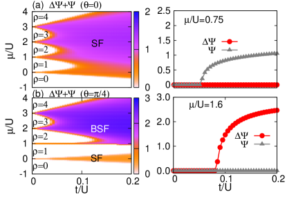
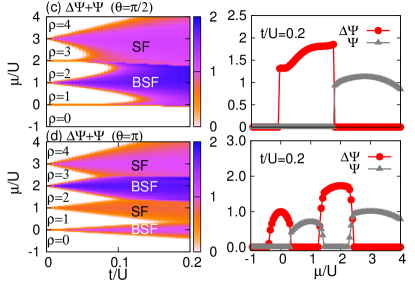
Figure 2: (Color online) The quantum phase ( $\Psi+\Delta\Psi$), which contains the SF, BSF and MI phases in the plane ($t/U$, $\mu/U$) of the model with (a) $\theta=$ 0, (b) $\pi/4$, (c) $\pi/2$, and (d) $\pi$, on the left column, from top to bottom sequentially. The right column are detailed descriptions of $\Psi$ and $\Delta\Psi$ along $t/U$ or $\mu/U$.

In this section, we present the global phase diagrams, by plotting $\Psi+\Delta\Psi$ in the plane ($t/U$, $\mu/U$) for $\theta$ at $0$, $\pi/4$, $\pi/2$ and $\pi$. The phase diagrams contain the SF and BSF phases and the staggered distribution between both phases. Fig. 2 (left) shows the phase diagrams of the model, the right column shows the detailed descriptions of $\Psi$ and $\Delta\Psi$ along $t/U$ or $\mu/U$.

At small $t/U$, with the maximum on-site occupation being $n_{max}=4$, the MI phases emerge sequentially with densities $\rho=0,1,2,3$ and $4$ when the chemical potential $\mu/U$ increases from $0$ to $4$.

At larger $t/U$, the system sits in the SF phase or the BSF phase, which are labeled in the phase diagrams. In the work of Ref. sta , the SF-MI phase transition boundaries have been obtained with $t/U>0$ and different values of $\theta$. The boundary lines are consistent with the results of Ref. sta , which are not shown here.

In Fig. 2(a), for $\theta=0$, the SF phase emerges with finite values of $t/U$. As shown in the right column at $\mu/U=0.75$, in the range $t/U>0.05$ , the SF phase is localized with $\Psi\neq 0$ and $\Delta\Psi=0$. By increasing $t/U$, $\Psi$ changes continuously into a non-zero regime, which means the MI-SF phase transition is continuous.

For $\theta=\pi/4$, when compared with $\theta=0$, a staggered pattern emerges for the distribution between the BSF and SF phases. The BSF phase emerges in the top right part of the phase diagram, and the SF phase emerges in the lower part, respectively. At the same time, the BSF and SF phases are separated by the MI phases.

For $\theta=\pi/2$, the BSF and SF phases can join together. To show the details, we scan $\mu/U$ along a cut line $t/U=0.2$. In the region $-1\textless\mu/U\textless-0.2$, both quantities $\Psi$ and $\Delta\Psi$ are equal to zero. By increasing $\mu/U$, the quantity $\Delta\Psi$ becomes nonzero with an obvious jump. This jump is due to the finite size of the MF frame, and finally disappears according to the DMRG calculation (not shown). The phase transition is still continuous.

In Fig. 2(d), for $\theta=\pi$, more of the SF and BSF phases emerge from top to bottom. The phase transition between the BSF and SF phases is first order because of the jumps within $\Psi$ and $\Delta\Psi$.

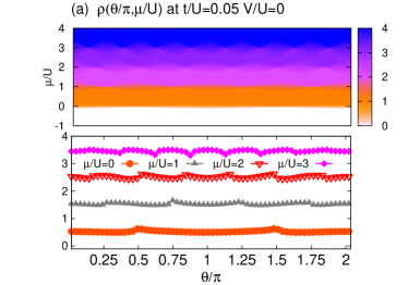
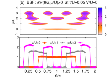
Figure 3: (Color online) The values of (a) density $\rho$ and (b) $\Delta\Psi$ in the plane ($\theta/\pi$, $\mu/U$) at $t/U=0.05$ and $V/U=0$. At the bottom of each figure (in color), we also plot the three quantities at $\mu/U=0$, 1, and 3 as a function of $\theta/\pi$ .

III.2 $t/U=0.05$: first-order BSF-SF phase transition

In the section above, we just show the quantities with four discrete values of $\theta$. Continuous modulation of $\theta$, Figs. 3 (a)-(b), show the quantities $\rho$ and $\Delta\Psi$ (from top to bottom, respectively) with the parameter plane ($\theta/\pi$, $\mu/U$) at $t/U=0.05$.

In Fig. 3 (a), the distribution of $\rho$ is shown as a function of $\theta/\pi$ and $\mu/U$. By increasing $\mu/U$ sequentially from 0 to 4, in the direction of $\mu/U$, the color becomes darker and darker, which means the density grows. We also find the “wave” along the boundaries between different colors (densities) along the $\theta/\pi$ direction. However, as we scan $\theta/\pi$ at the bottom of Fig. 3 (a), the densities have several kinks. The emergence frequency of the kinks increases as the density $\rho$ (chemical potential $\mu$) increases. The number of kinks for $\mu/U=0$, 1, 2 and 3 are 2, 4, 6 and 8, respectively.

For example, for $\mu/U=0$ by changing $\theta/\pi$, the density curve has two kinks at $\theta/\pi=0.5$ and 1.5. Actually the kinks emerge as a phase transition takes place. For larger $\mu/U$, the variation becomes more obvious. This phenomena can be understood by the following. According to $a_{j}=b_{j}exp(i\theta\sum_{i}^{j-1}n_{i})$, if the value of $\sum_{i}^{j-1}n_{i}$ is bigger, then the operator $a_{j}=b_{j}exp(i\theta\sum_{i}^{j-1}n_{i})$ will change more quickly as $\theta$ changes.

In Fig. 3 (b), the distribution of $\Delta\Psi$ is shown in the plane ($\mu/U$, $\theta/\pi$). All colored regions ($\Delta\Psi$) represent the BSF phase. For example, when $\mu/U=0$, $\Delta\Psi>0$ in a narrow area in the regime $0.5<\theta/\pi<1.5$. We also show $\Delta\Psi$ at $\mu/U=0,1$ and 3 along $\theta/\pi$, which confirms the result from Fig. 3 (a). An obvious first-order SF-BSF phase transition is found because of the jumps of the order parameters. The distribution of $\Psi$ and the details are not shown here.

IV DMRG Results

IV.1 Phase diagrams

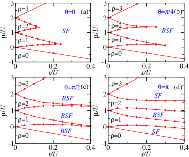
Figure 4: (Color online) The DMRG phase diagrams, which contains the SF, BSF and MI phases in the plane ($t/U$, $\mu/U$) of the model with (a) $\theta=0$, (b) $\pi/4$, (c) $\pi/2$ and (d) $\pi$.

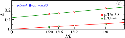
Figure 5: (Color online) (a) Correlation C(r) with system size $L=16$, $t/U=4$, $\theta=\pi$ in the SF phase at $\mu/U=-4.07$ and in the BSF phase with $\mu/U=-3.76$, (b) $\Delta$ .vs. $\mu/U$ with system sizes $L=12,16$.

Fig. 4 shows the phase diagrams, which contain the SF, BSF and MI phases in the plane ($t/U$, $\mu/U$) of the model with $\theta=0,\pi/4,\pi/2$, and $\pi$.

For $\theta=0$, only the SF phase emerges. This is very consistent with the corresponding result in the MF frame, as shown in Fig. 2 (a).

For $\theta=\pi/4$ and $\pi/2$, the MF phase diagrams contain both the SF and BSF phases. However, compared with Fig. 2, the DMRG only detects the BSF phases. The SF phase detected by MF method is actually the BSF phase, where the wavelengths of the waves emerging in the correlation are too long to be detected by the MF method.

For $\theta=\pi$, the stagger distributions of the SF and BSF phases are also found by the DMRG calculation.

With larger $t$ (for example $t/U=4$), the direct SF-BSF phase transitions occur. In Fig. 5 (a), two typical correlations of both the SF and BSF phases are shown. In the BSF phase, the correlation exhibits obvious oscillations, which can be roughly characterized by $\Delta=C(L/2)-C(L/2-1)$. Clearly, $\Delta\neq 0$ emerges in the BSF phase and $\Delta=0$ emerges in the SF phase. In Fig. 5 (b), we find $\Delta=0$ if $\mu/U\textless-3.94$ while $\Delta\neq 0$ when $\mu/U>-3.94$ in the thermodynamic limit. The finite size scaling analysis is performed at $\mu/U=-4$ and $-3.8$ as shown in Fig. 5(c). Although there is no rough jump of the order parameter $\Delta$, in contradistinction to the MF prediction, one can still observe a direct phase transition between the two type of superfluid phases.

IV.2 Beat and Correlation

To clearly see the effects of $\theta\neq 0$, we choose $\theta=\pi/2$. In this case, more interesting properties emerge. Firstly, no homogenous SF phase exists. Except for the MI phases with different fillings, all regimes are in the BSF phase. This is obviously different from the MF result in Fig. 2 (b).

The properties of the BSF phase are studied by plotting the correlation along $t/U=0.4$ from $\mu/U=-0.5$ to $\mu/U=3$ at some intervals, is chosen to show in Fig. 6. The first finding is the beat phenomena emerging from the correlation. Furthermore, the oscillation period of the correlation becomes longer or shorter as the density (chemical potential) changes. Moreover, the type of behavior of the correlation emerges in a staggered pattern in the phase diagram.

The superposition of two waves of the same frequency propagating in opposite directions will cause a standing wave, in which the maximum amplitude and minimum amplitude are constants. If the two waves have slightly different frequencies, beats will forms, in which the maximum and minimum amplitudes are no longer constants.

Fig. 6 (a) shows the real part of the correlation $C(r)$ at $\mu/U=-0.25$ and $t/U=0.4$ with size $L=60$. Clearly, the sign of the correlation oscillates as the distance $r$ grows between the two sites. It behaves in a triangular wave shape with a beat. The correlation increases once and decreases once, backwards and forwards, where the oscillation wavelength is $\lambda_{1}=2$, and the beat wavelength is $\lambda_{2}=18$. In the position $r=16$, the amplitude tends to zero, where zero is the node of a beat. Beyond the node, the amplitude grows again and a new beat starts again. Even at the ends, beats are discernable, because the nodes and maximum are observable.

Fig. 6 (b) shows the imaginary part of the correlation $C(r)$. The positions of the nodes in the real part of $C(r)$ correspond to the peaks or the lowest positions in the imaginary part.

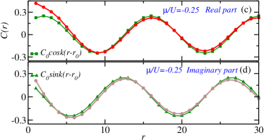
Figure 6: (Color online) Correlations $C(r)$ for $L=60$, $m=80$ $\theta=\pi/2$, $t/U=0.4$. (a) Real part of $C(r)$ with $\mu/U=2$ (b) Imaginary part $C(r)$ with $\mu/U=2$ (c) Real part of $C(r)$ with $\mu/U=-0.25$ (d) Imaginary part $C(r)$ with $\mu/U=-0.25$. In (a), $\lambda_{1}$ and $\lambda_{2}$ are the oscillation wavelength and beat wavelength respectively. The green lines are plotted to emphasize the beats.

In the mean-field frame, we assume only a two-sublattice structure as a possible inhomogeneity in the ground state. However, due to the existence of the phase factor $\theta$ of model (3), it is naturally expected that a state with a longer (incommensurate) wavelength can appear. For example, the order parameters may have uniform amplitude but with a “spiral” phase factor, i.e., $\Psi\propto|\Psi|e^{ikr}$. The DMRG method can overcome the constraint from the MF method. From our calculation, $C(r)$ realy emerges according to a pattern of

$$C(r)=C_{0}e^{ik(r-r_{0})}.$$ (7)

For example, in the case of the green lines of Figs. 6(c) and (d), $C_{0}=0.25$ and $k=0.4488$ are used. Here, $r_{0}=2$ and $r_{0}=9$ are for the real and imaginary parts, respectively. Furthermore, in Figs. 6 (a) and (b), the correlation $C(r)$ in the shape of the beats obey the equation as follows

$$C(r)=C_{0}e^{ik(r-r_{0})}(-1)^{r}.$$ (8)

For $\mu/U=1.5$, the wavelengths of the beats $\lambda_{2}$ become shorter $\lambda_{2}=10$. From $\mu/U=0.5$ to $-0.5$, $\lambda_{2}$ disappears and therefore beats don’t exist. The value of the oscillation wavelength $\lambda_{1}$ is still present.

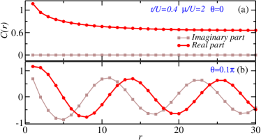
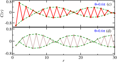
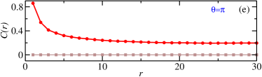
Figure 7: (Color online) Emergence and disappearance of beats from both of the real and imaginary parts of the correlation $C(r)$ by modulation of $\theta$ for $\theta/\pi=0$, $0.1$, $0.6$ and $1$ at $t/U=0.4$, $\mu/U=2$.

Apart from the notion that $\mu/U$ or the density will change the properties with or without beats, the effects of $\theta$ upon the correlation need to be discussed. In Figs. 7 (a)-(d), we start with a SF phase, at $t/U=0.4$, $\mu/U=2$, and $\theta=0$, no oscillation in the correlation exists. We then increase $\theta/\pi$ from $0$ to $1$ with a spacing of $0.1$. When $\theta=0.1\pi$, the correlation oscillates smoothly. When $\theta=0.6\pi$, beats emerge. Beats disappear at $\theta=\pi$.

To summarise, for $0\textless\theta\textless\pi$, the BSF phase emerges and beats emerges for a range of values of $\mu/U$.

IV.3 Explanation of beats by the momentum distribution

The reason why beats exists in Fig. 6 (a) or do not exist in Fig. 6 (b) can be analyzed by the momentum distributions. Figs. 8 (a) and (b) show the momentum distributions $n(k)$ with the same parameters as those of Figs. 6, which are helpful to us in understanding the behavior of the correlations. On the whole, the two peaks of the momentum distribution reflect the wave numbers ${k}_{1}$ and ${k}_{2}$, which superpose together to form various kinds of correlation patterns. The condition for beat existence is given by $y=\frac{{k}_{1}-{k}_{2}}{{k}_{1}+{k}_{2}}<\frac{1}{3}$ (see appendix).

To check the correction of the momentum distribution obtained, we sum $n(k)$ over different values of the wave numbers ${k}$ as follows

$$\sum_{m=1}^{L}n(k=\dfrac{2m\pi}{L})=L\rho=N,$$ (9)

where $L$ is the chain length and $N$ is the number of total particles. Our numerical values are very consistent with the above equation.

Table 1: Values of $\lambda_{1}$, $k_{1}^{{}^{\prime}}/\pi$, $k_{1}/\pi$, $\lambda_{2}$, $k_{2}^{{}^{\prime}}/\pi$, and $k_{2}/\pi$ in Fig. 8. $\lambda_{1}$ and $\lambda_{2}$ are the oscillation and beat wavelengths, respectively. $k_{1}$ and $k_{2}$ are from the peaks of momentum distributions. $k_{1}^{{}^{\prime}}$ and $k_{2}^{{}^{\prime}}$ are from the real space correlation.

$\mu/U$	$\lambda_{1}$	$k_{1}^{{}^{\prime}}/\pi$	$k_{1}/\pi$	$\lambda_{2}$	$k_{2}^{{}^{\prime}}/\pi$	$k_{2}/\pi$	$y$
1.5	2	1.20	1.17	10	0.80	0.83	0.17
2.0	2	1.11	1.10	18	0.89	0.90	0.1
2.5	2	1.06	1.03	34	0.94	0.97	0.03
$-0.5$			1.97			0.03	0.97
$-0.25$			1.87			0.13	0.87
0.0			1.73			0.27	0.73
0.5			1.43			0.57	0.43

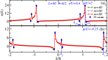
Figure 8: (Color online) Asymmetric momentum distribution $n(k)$ by DMRG calculations with the same parameters in Figs. 6. (a)$k_{1}=1.1$ and $k_{2}=0.9$, satisfying the existing of beats $y<1/3$; (b) $k_{1}=1.87$ and $k_{2}=0.13$, which does not satisfy $y<1/3$.

In Fig. 8 (a), for $\mu/U=2$, the peaks $k_{1}$ and $k_{2}$ can be obtained from the momentum distribution as shown in table 1, where $k_{1}=1.1$ and $k_{2}=0.9$. Beats form clearly because $y=0.1\textless 1/3$. To check the correctness of $k_{1}$ and $k_{2}$, the peaks can also be compared with $k_{1}^{{}^{\prime}}$ and $k_{2}^{{}^{\prime}}$ by deviation from the oscillation lengths $\lambda_{1}$ and the beat length $\lambda_{2}$ in real space. The flow chart is as follow,

$$\lambda_{1},\lambda_{2}\Rightarrow k_{quick},k_{slow}\Rightarrow k_{1}^{{}^{\prime}},k_{2}^{{}^{\prime}}\Longleftrightarrow k_{1},k_{2}.$$ (10)

We assume a beat, resulting from two superposed waves with slightly different frequencies $k_{1}^{{}^{\prime}}$ and $k_{2}^{{}^{\prime}}$, then we will obtain a beat with an oscillation frequency $k_{quick}=\frac{k_{1}^{{}^{\prime}}+k_{2}^{{}^{\prime}}}{2}$ and a beat frequency $k_{slow}=\frac{k_{1}^{{}^{\prime}}-k_{2}^{{}^{\prime}}}{2}$, where $k_{quick}$ and $k_{slow}$ can be obtained by counting $\lambda_{1}$ and $\lambda_{2}$, where $k_{quick}=\frac{2\pi}{\lambda_{1}}$ and $k_{slow}=\frac{2\pi}{\lambda_{2}}$.

Apparently, as shown in table 1, by comparing each of the wave numbers ${k}_{i}$ ($i=1,2$) of the same index in table 1, we find that $k_{1}$ and $k_{1}^{\prime}$, and $k_{2}$ and $k_{2}^{\prime}$ are fairly close to each other to within the first two digits. Two ways of obtaining the frequencies of the two superposed waves are checked against each other. The finite size effects and quantum fluctuation make ${k}_{i}$ and ${k}_{i}^{\prime}$ ($i=1,2$) a little different.

Fig. 8 (b) shows that, at $\mu/U=-0.25$, two separated peaks far apart from each other emerge around $k_{2}/\pi=0$ and $k_{1}/\pi=2$, where the wave numbers ${k}_{1}$ and ${k}_{2}$ are available in Table 1. In real space, the beat phenomena does not exist as shown in Fig. 6 (b) with the same parameters. The reason is not that the length of the beat is too long to be seen in a limited size $L=60$, where $L$ is supposed to be the length of the system. Rather it is because the two wave numbers ${k}_{1}$ and ${k}_{2}$ do not satisfy the condition for existence of the beat.

IV.4 Asymmetry of momentum distribution

In table 1, numerical results mean that the sums over ${k}_{1}$ and ${k}_{2}$ remain at $2\pi$ and the two wave numbers are symmetric with $k/\pi=1$. However, the shapes of the momentum distributions are asymmetric with $k=0$. The reflectional symmetry about $k=0$ is broken because of the asymmetric phase factor assigned to the hopping. The asymmetry is consistent with the results in Refsground1 ; ground2 ; tang .

To understand the asymmetry of the momentum distribution, the asymmetry of the energy spectrum in momentum space is given. It is well known that, when $\theta=0$, the energy of the non interacting Bose-Hubbard model with Hamiltonian $H^{b}=-t\sum_{i=1}^{L}(b^{\dagger}_{i}b_{i+1}e^{i\theta n_{i}}+h.c.)$ is $E(k)=-2t\cos(k)$, which is obviously symmetric about $k/\pi=0$. In the derivation, the relationship

$$\sum_{i}(b^{\dagger}_{i}b_{i+1}+b^{\dagger}_{i}b_{i-1})=\sum_{k}b^{\dagger}_{k}b_{k}(e^{ik}+e^{-ik})$$ (11)

is usedsolidth . For a system with a fixed density, $n_{i}$ is a constant $\overline{n}_{i}$. Letting $e^{i\theta\overline{n}_{i}}$ couple the eq. (11), we get

$$\sum_{i}(b^{\dagger}_{i}b_{i+1}e^{i\theta\overline{n}_{i}}+b^{\dagger}_{i}b_{i-1}e^{-i\theta\overline{n}_{i}})$$ (12)

$$=\sum_{k}b^{\dagger}_{k}b_{k}(e^{ik+i\overline{n}_{i}\theta}+e^{-ik-i\overline{n}_{i}\theta})$$

Therefore, $E(k)=-2t\cos(k+\theta\,\overline{n}_{i})$ and should be asymmetric with $k=0$ if $\theta\,\overline{n}_{i}\neq 0$ .

V Discussion and conclusion

By using the DMRG and MF methods, the anyon Hubbard model has been studied systematically on a one dimensional lattice.

The MF method can provide us with the basic phase diagrams, which are consistent with the results from the DMRG method with $\theta/\pi=0$. For other values of $\theta$, although the MF method cannot provide the precise phase-diagrams, the MF method still help us search for the different behaviors of the correlations.

The concept of broken-symmetry plays an important role in theoretical physics, such as in the origin of the mass associated with the Higgs bosonbs1 . Here, various interesting patterns of the correlation $b^{+}_{i}b_{i+r}$ enrich the concept of broken-symmetry in correlated boson systems. In some areas, the correlation yields beats if the two supposing wave numbers ${k}_{1}$ and ${k}_{2}$ satisfy $({k}_{1}-{k}_{2})/({k}_{1}+{k}_{2})<1/3$.

We never see beats in the correlation $b^{\dagger}_{i}b_{i+r}$ for the usual Bose-Hubbard model except the solid order patternsoli . Note that this work is the first to observe beats of the correlation $b^{\dagger}_{i}b_{i+r}$ in the Bose-Hubbard type model. Different kinds of momentum distributions are analysed and expected to be observed in optical lattice experiments.

Appendix A the standard $y<1/3$

Here, we show how to get the criteria of existence of a beat, namely, $y<1/3$. We assume a beat mixed with two waves with wave numbers ${k}_{1}^{{}^{\prime}}$ and ${k}_{2}^{{}^{\prime}}$, respectively. The difference of the two wave numbers should be less than the sum of both wave numbers, namely

$$k_{1}^{{}^{\prime}}-k_{2}^{{}^{\prime}}<k_{1}^{{}^{\prime}}+k_{2}^{{}^{\prime}}.$$ (13)

For convenience, we let $y=\frac{k_{1}^{{}^{\prime}}-k_{2}^{{}^{\prime}}}{k_{1}^{{}^{\prime}}+k_{2}{{}^{\prime}}}<1$, and $k_{1}{{}^{\prime}}=ak_{2}^{{}^{\prime}}$. Then we assume $\dfrac{k_{1}{{}^{\prime}}}{k_{2}^{{}^{\prime}}}=a>1$, which leads to

$$y=\dfrac{ak_{2}^{{}^{\prime}}-k_{2}^{{}^{\prime}}}{ak_{2}^{{}^{\prime}}+k_{2}{{}^{\prime}}}=\dfrac{a-1}{a+1}<1$$ (14)

Now, we discuss the possible value of $a$. Firstly, a beat will not exist if the two wave numbers are the same, ie., $a=1$ or one of the wave numbers ${k}_{1}^{{}^{\prime}}$ is twice as much as that of the other wave numbers ${k}_{2}^{{}^{\prime}}$, namely, $a=2$. A reasonable choice of $a$ is $1<a<2$ and then we can easily obtain $0<y<\dfrac{1}{3}$ beat .

Appendix B Comparison with Greschner Data

To check correctness of our findings, we compare the data of $C(r)$ with the same boundary conditions (periodic boundary conditions) from the data of Greschner, an author of Ref. santos2 . The parameters are $L=60$, $U=2.5$, $t=1$ and $n_{max}=4$. Both data have beats and are basically consistent with each other quantitatively although we used $\mu/U=3.3455$ and the number of the particle is $N_{total}=137$ and S. Greschner used $N_{total}=139$.

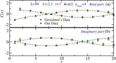
Figure 9: (Color online) Comparison of our data $C(r)$ with the result from S. Greschnersantos2 .