On the Role of Artificial Noise in Training and
Data Transmission for Secret Communications

Abstract

This work considers the joint design of training and data transmission in physical-layer secret communication systems, and examines the role of artificial noise (AN) in both of these phases. In particular, AN in the training phase is used to prevent the eavesdropper from obtaining accurate channel state information (CSI) whereas AN in the data transmission phase can be used to mask the transmission of the confidential message. By considering AN-assisted training and secrecy beamforming schemes, we first derive bounds on the achievable secrecy rate and obtain a closed-form approximation that is asymptotically tight at high SNR. Then, by maximizing the approximate achievable secrecy rate, the optimal power allocation between signal and AN in both training and data transmission phases is obtained for both conventional and AN-assisted training based schemes. We show that the use of AN is necessary to achieve a high secrecy rate at high SNR, and its use in the training phase can be more efficient than that in the data transmission phase when the coherence time is large. However, at low SNR, the use of AN provides no advantage since CSI is difficult to obtain in this case. Numerical results are presented to verify our theoretical claims.

I Introduction

Information-theoretic secrecy has received renewed interest in recent years, especially in the context of wireless communications, due to the broadcast nature of the wireless medium and the increasing amount of confidential data that is being transmitted over the air. Most of these studies stem from the seminal works by Wyner in [1] and by Csiszar and Korner in [2], where the so-called secrecy capacity was characterized for degraded and nondegraded discrete memoryless wiretap channels (i.e., channels consisting of a source, a destination, and a passive eavesdropper), respectively. The notion of secrecy capacity was introduced in these works as the maximum achievable secrecy rate between the source and the destination subject to a constraint on the information attainable by the eavesdropper. These issues were also examined for Gaussian channels by Leung-Yan-Cheong and Hellman in [3], where Gaussian signalling was shown to be optimal. These works show that the secrecy capacity of a wiretap channel increases with the difference between the channel quality at the destination and that at the eavesdropper.

In recent years, studies of the wiretap channel have also been extended to multi-antenna wireless systems, e.g., in [4, 5, 6, 7, 8], where the achievable secrecy rates were examined under different channel assumptions and techniques were proposed to best utilize the available spatial degrees of freedom. In particular, the work in [4] examined the secrecy capacity of a multiple-input single-output (MISO) wiretap channel and showed that transmit beamforming with Gaussian signalling is optimal. However, perfect knowledge of both the main and the eavesdropper channel state information (CSI) was required at the source in order to determine the optimal beamformer. In [5, 6, 7, 8], more general results were obtained for cases with multiple antennas at the destination. Precoding techniques were proposed as a generalization of the beamforming scheme in [4] to higher dimensions and, thus, perfect CSI of all links was also required to derive the optimal precoder. On the other hand, when the eavesdropper CSI is unavailable, which is often the case in practice, the secrecy capacity and its corresponding optimal transmission scheme are both unknown. However, an artificial noise (AN) assisted secrecy beamforming scheme, where data is beamformed towards the destination and AN is placed in the null space of the main channel direction to jam the eavesdropper’s reception, is often adopted and was in fact shown to be asymptotically optimal in [4]. Even though knowledge of the eavesdropper channel is not required in this transmission scheme, perfect knowledge of the main channel CSI is still needed, which can also be unrealistic due to the presence of noise in the channel estimation.

In practice, CSI is typically obtained through training and channel estimation at the destination. In conventional systems (without secrecy constraints), training signal designs have been studied in the literature for both single-user [9, 10] and multiuser systems [11]. In these cases, training is often done by having the source transmit a pilot signal to enable channel estimation at the destination (and CSI at the source is obtained by having the destination feedback its channel estimate to the source). However, this approach may not be favorable for systems with secrecy considerations since the emission of pilot signals by the source also enables channel estimation at the eavesdropper (and in this way enhances its ability to intercept the source’s message). More recently, a secrecy enhancing training scheme, called the discriminatory channel estimation (DCE) scheme, was proposed in [12, 13], where AN is super-imposed on top of the pilot signal in the training phase to disrupt the channel estimation at the eavesdropper. These works showed that DCE can indeed enhance the difference between the channel estimation qualities at the destination and the eavesdropper in the training phase (before the actual data is transmitted), but did not discuss its impact on the achievable secrecy rate in the data transmission phase.

The main objective of this work is to examine the impact of both conventional and DCE-type training on the achievable secrecy rate of AN-assisted secrecy beamforming schemes. Different from previous works in the literature that focus on either training or data transmission, we consider the joint design and examine the role of AN in both of these phases. In this work, the two-way DCE scheme proposed in [13] is employed in the training phase to prevent CSI leakage to the eavesdropper, and the AN-assisted secrecy beamforming scheme is used in the data transmission phase to mask the transmission of the confidential message. We first derive bounds on the achievable secrecy rate of these schemes, which are shown to be asymptotically tight as the transmit power increases, and utilize them to obtain closed-form approximations of the achievable secrecy rate. Then, based on the approximate secrecy rate expressions, optimal power allocation policies for the pilot signal, the data signal, and AN in both phases are obtained for systems employing conventional and AN-assisted training schemes, respectively. We show that the use of AN (in either training or data transmission) is often necessary to achieve a significantly higher secrecy rate at high SNR, and that its use in training can be more efficient than that in data transmission when the coherence time is long. However, in the low SNR regime, the use of AN provides no advantage in either training or data transmission. In fact, allocating resources for training can be strictly suboptimal in this regime since it is difficult to obtain useful CSI when power is scarce. Numerical results are provided to verify our theoretical claims.

The joint design of training and data transmission have been investigated for conventional MIMO point-to-point and multiuser scenarios (without secrecy constraints) in [14] and [15], respectively. However, these issues have not been discussed before for physical layer secret communications, where finding a reasonable approximation for the achievable secrecy rate under channel estimation errors, and coping with the non-Gaussianity caused by the combination of AN and channel estimation errors can be challenging. The impact of imperfect CSI due to channel estimation errors and limited feedback on the achievable secrecy rate have been examined in [16, 17] and [18], respectively. However, these works focus on the achievable secrecy rate for given estimation error statistics without consideration on how training should be performed and how it can impact the error statistics. Moreover, CSI at the eavesdropper is often assumed to be perfect in these works to avoid the need to analyze the impact of channel estimation error at the eavesdropper. A preliminary study of our work was presented in [19] for the case of conventional training. The current work further considers the case of AN-assisted training, provides rigorous proofs of the theoretical claims, and examines the low SNR case.

The remainder of this paper is organized as follows. In Section II, the system model and the training-based transmission scheme are introduced. In Section III, upper and lower bounds of the achievable secrecy rate under channel estimation error are obtained. In Sections IV and V, closed-form secrecy rate expressions and optimal power allocation policies are derived for cases with conventional and DCE training, respectively. The analysis of the secrecy rate with training-based transmission scheme in the low SNR regime is discussed in Section VI. Finally, numerical results are provided in Section VII, and a conclusion is given in Section VIII.

II System Model

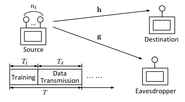
Figure 1: Training-based secret transmission scheme that consists of a training phase and a data transmission phase.

Let us consider a wireless secret communication system that consists of a source, a destination, and an eavesdropper. The source is assumed to have $n_{t}$ antennas whereas both the destination and the eavesdropper are assumed to have only a single antenna each. The main and eavesdropper channels (i.e., the channel from the source to the destination and to the eavesdropper, respectively) can be described by the vectors $\mathbf{h}=[h_{1},\ldots,h_{n_{t}}]^{T}$ and $\mathbf{g}=[g_{1},\ldots,g_{n_{t}}]^{T}$, respectively, where the entries are assumed to be independent and identically distributed (i.i.d.) complex Gaussian random variables with mean $0$ variances $\sigma_{h}^{2}$ and $\sigma_{g}^{2}$, respectively (i.e., ${\cal CN}(0,\sigma_{h}^{2})$ and ${\cal CN}(0,\sigma_{g}^{2})$). We consider a block fading scenario where the channel vectors remain constant over a coherence interval of duration $T$, but vary independently from block to block. By adopting a training-based transmission scheme, each coherence interval is divided into a training phase with duration $T_{t}$ and a data transmission phase with duration $T_{d}$, as illustrated in Fig. 1. In the training phase, pilot signals are emitted by the source (and/or the destination) to enable channel estimation at the destination; and, in the data transmission phase, confidential messages are transmitted utilizing the estimated channel obtained in the previous phase. Following methods proposed in [12, 13] for training and in [20] for data transmission, AN is utilized in the respective phases to degrade the reception at the eavesdropper. Our goal is thus to determine the optimal resource allocation between signal and AN, and examine the role of AN in these two phases.

II-A Training Phase - AN-Assisted Training

In conventional point-to-point communication systems, training is typically performed by having the source emit pilot signals to enable channel estimation at the destination. Most works in the literature on physical layer secrecy, e.g., [4, 20, 21, 22], inherit such an assumption and, thus, assume that the eavesdropper can also benefit from the pilot transmission and can obtain a channel estimate that is no worse than the destination. Interestingly, it has been shown more recently in [12, 13] that secrecy can be further enhanced by embedding AN in the pilot signal to degrade the channel estimation performance at the eavesdropper. By doing so, the difference between the effective channel qualities experienced by the destination and the eavesdropper can be enhanced and, thus, a higher secrecy rate can be achieved. Here, we consider in particular the two-way discriminatory channel estimation (DCE) scheme proposed in [13]. In the DCE scheme, training is performed in two stages, i.e., the reverse and the forward training stages. In the reverse training stage, a pure pilot signal is sent in the reverse direction by the destination to enable channel estimation at the source; in the forward training stage, a pilot signal masked by AN is emitted by the source to facilitate channel estimation at the destination while preventing reliable channel estimation at the eavesdropper. Here, the channel is assumed to be reciprocal, that is, the reverse channel can be represented as the transpose of the forward channel vector, i.e., $\mathbf{h}^{t}$. Therefore, estimation of the reverse channel provides the source with information about the forward channel. Note that DCE can also be used in non-reciprocal channels, as shown in [13], but is not considered here for simplicity.

Let $T_{r}$ and $T_{f}$ be the length of the reverse and the forward training stages, respectively, where $T_{r}+T_{f}=T_{t}$. In the reverse training stage, the pilot signal $\mathbf{s}_{r}\in\mathcal{C}^{T_{r}\times 1}$ with $\mathbf{s}_{r}^{{\dagger}}\mathbf{s}_{r}=T_{r}$ is first emitted by the destination and the received signal at the source can be written as

$$\mathbf{Y}_{r}=\sqrt{P_{r}}\,\mathbf{s}_{r}\mathbf{h}^{t}+\mathbf{V}_{r}$$ (1)

where $P_{r}$ is the power of the pilot signal in the reverse training stage, $\mathbf{h}^{t}$ is the channel vector from the destination to the source, and $\mathbf{V}_{r}\in\mathcal{C}^{T_{r}\times n_{t}}$ is the additive white Gaussian noise (AWGN) matrix with entries that are i.i.d. $\mathcal{CN}(0,\sigma^{2})$. Following the procedures given in [13], the source first computes the minimum mean square error (MMSE) estimate of the channel based on the knowledge of $\mathbf{s}_{r}$. The channel estimate at the source is denoted by $\mathbf{\widetilde{h}}$ and the channel estimation error is $\mathbf{\Delta h}_{r}=\mathbf{h}-\mathbf{\widetilde{h}}$. The variance of each entry of $\mathbf{\Delta h}_{r}$ can be written as

$$\sigma_{\Delta h_{r}}^{2}=\left(\frac{1}{\sigma_{h}^{2}}+\frac{P_{r}T_{r}}{\sigma^{2}}\right)^{-1}.$$ (2)

Then, in the forward training stage, the source emits a training signal with AN placed in the null space of the estimated forward channel, i.e., $\mathbf{\widetilde{h}}$. The signal transmitted in the forward training stage is given by

$$\mathbf{X}_{f}=\sqrt{P_{f}}\mathbf{S}_{f}+\mathbf{A}_{f}\mathbf{N}_{\widetilde{\mathbf{h}}},$$ (3)

where $\mathbf{S}_{f}\in\mathcal{C}^{T_{f}\times n_{t}}$ is the pilot signal in the forward training stage with $\mathbf{S}^{{\dagger}}_{f}\mathbf{S}_{f}=\frac{T_{f}}{n_{t}}\mathbf{I}$, $P_{f}$ is the power of the pilot signal in the forward training stage, $\mathbf{N}_{\widetilde{\mathbf{h}}}\in\mathcal{C}^{(n_{t}-1)\times n_{t}}$ is a matrix whose rows span the null space of $\mathbf{\widetilde{h}}$ and satisfies $\mathbf{N}_{\widetilde{\mathbf{h}}}\mathbf{N}^{{\dagger}}_{\widetilde{\mathbf{h}}}=\mathbf{I}_{n_{t}-1}$, and $\mathbf{A}_{f}\in\mathcal{C}^{T_{f}\times(n_{t}-1)}$ is the AN with entries that are i.i.d. $\mathcal{CN}(0,\frac{P_{f_{a}}}{n_{t}-1})$. Hence, the total AN power in the forward training stage is $P_{f_{a}}$. The signals received at the destination and the eavesdropper can then be written respectively as

$$\mathbf{y}_{f} =\mathbf{X}_{f}\mathbf{h}+\mathbf{v}_{f}=\sqrt{P_{f}}\mathbf{S}_{f}\mathbf{h}+\mathbf{A}_{f}\mathbf{N}_{\widetilde{\mathbf{h}}}\mathbf{\Delta h}_{r}+\mathbf{v}_{f},$$ (4)

$$\mathbf{z}_{f} =\mathbf{X}_{f}\mathbf{g}+\mathbf{w}_{f}=\sqrt{P_{f}}\mathbf{S}_{f}\mathbf{g}+\mathbf{A}_{f}\mathbf{N}_{\widetilde{\mathbf{h}}}\mathbf{g}+\mathbf{w}_{f},$$ (5)

where $\mathbf{v}_{f}$ and $\mathbf{w}_{f}$ are the AWGN with entries that are i.i.d. $\mathcal{CN}(0,\sigma^{2})$ at the destination and the eavesdropper, respectively. The destination and the eavesdropper are then able to compute MMSE estimates $\mathbf{\hat{h}}$ and $\mathbf{\hat{g}}$ of their respective channels. The channel estimation error vectors are $\mathbf{\Delta h}\triangleq\mathbf{h}-\mathbf{\hat{h}}$ and $\mathbf{\Delta g}\triangleq\mathbf{g}-\mathbf{\hat{g}}$, whose entries are $0$ mean with variances

$$\sigma^{2}_{\Delta h} =\left(\frac{1}{\sigma_{h}^{2}}+\frac{P_{f}T_{f}/n_{t}}{P_{f_{a}}\sigma_{\Delta h_{r}}^{2}+\sigma^{2}}\right)^{-1},$$ (6)

and

$$\sigma^{2}_{\Delta g} =\left(\frac{1}{\sigma_{g}^{2}}+\frac{P_{f}T_{f}/n_{t}}{P_{f_{a}}\sigma_{g}^{2}+\sigma^{2}}\right)^{-1},$$ (7)

respectively. The channel estimate $\hat{\mathbf{h}}$ is fed back to the source for use in data transmission.

It is interesting to remark that, in the DCE scheme described above, reverse training is first performed to provide the source with knowledge of the channel between itself and the destination (but does not help the eavesdropper obtain information about its channel from the source). This knowledge is then used by the source to determine the AN placement in the forward training stage so as to minimize its interference at the destination. In conventional training, only the forward training stage is required since AN is not utilized. In this case, the training length is $T_{t}=T_{f}$ (since $T_{r}=0$) and the forward training signal can be expressed simply as $\mathbf{X}_{f}=\sqrt{P_{f}}\mathbf{S}_{f}$. Even though the time required for conventional training is less than that of DCE (leaving more channel uses for data transmission in each coherence interval), the achievable secrecy rate may not necessarily be higher due to increased CSI leakage [22] to the eavesdropper.

II-B Data Transmission Phase - AN-Assisted Secrecy Beamforming

Suppose that the source is able to obtain knowledge of the channel estimate $\hat{\mathbf{h}}$ through feedback from the destination but has only statistical knowledge of the eavesdropper’s channel $\mathbf{g}$ (and also $\hat{\mathbf{g}}$). Based on this channel knowledge, the source can then utilize in the data transmission phase an AN-assisted secrecy beamforming scheme [20] where the data-bearing signal is directed towards the destination while AN is placed in the null space of $\hat{\mathbf{h}}$ to jam the reception at the eavesdropper. The transmit signal is thus given by

$$\mathbf{X}_{d}=\sqrt{P_{d}}\,\mathbf{s}_{d}\mathbf{\frac{\hat{h}^{{\dagger}}}{\|\hat{h}\|}}+\mathbf{A}_{d}\mathbf{N}_{\hat{\mathbf{h}}}$$ (8)

where $\mathbf{s_{d}}\in\mathcal{C}^{T_{d}\times 1}$ is the data-bearing signal vector whose entries are i.i.d. $\mathcal{CN}(0,1)$, $P_{d}$ is the power of the data signal, $\mathbf{N}_{\hat{\mathbf{h}}}\in\mathcal{C}^{(n_{t}-1)\times n_{t}}$ is the matrix that spans the null space of $\mathbf{\hat{h}}$ and satisfies $\mathbf{N}_{\hat{\mathbf{h}}}\mathbf{N}^{{\dagger}}_{\hat{\mathbf{h}}}=\mathbf{I}_{n_{t}-1}$, and $\mathbf{A}_{d}\in\mathcal{C}^{T_{d}\times(n_{t}-1)}$ is the AN matrix whose entries are i.i.d. $\mathcal{CN}(0,\frac{P_{a}}{n_{t}-1})$. Hence, the total AN power in the data transmission phase is $P_{a}$.

The signals received at the destination and the eavesdropper are given by

$$\mathbf{y}_{d} =\mathbf{X}_{d}\mathbf{\hat{h}}+\mathbf{X}_{d}\mathbf{\Delta h}+\mathbf{v}_{d}=\sqrt{P_{d}}\,\mathbf{s}_{d}\mathbf{\|\hat{h}\|}+\sqrt{P_{d}}\,\mathbf{s}_{d}\mathbf{\frac{\hat{h}^{{\dagger}}}{\|\hat{h}\|}}\mathbf{\Delta h}+\mathbf{A}_{d}\mathbf{N}_{\hat{\mathbf{h}}}\mathbf{\Delta h}+\mathbf{v}_{d},$$ (9)

$$\mathbf{z}_{d} =\mathbf{X}_{d}\mathbf{\hat{g}}+\mathbf{X}_{d}\mathbf{\Delta g}+\mathbf{w}_{d}=\sqrt{P_{d}}\,\mathbf{s}_{d}\mathbf{\frac{\hat{h}^{{\dagger}}}{\|\hat{h}\|}}\mathbf{\hat{g}}+\sqrt{P_{d}}\,\mathbf{s}_{d}\mathbf{\frac{\hat{h}^{{\dagger}}}{\|\hat{h}\|}}\mathbf{\Delta g}+\mathbf{A}_{d}\mathbf{N}_{\hat{\mathbf{h}}}\mathbf{g}+\mathbf{w}_{d},$$ (10)

where $\mathbf{v}_{d}\sim\mathcal{CN}({\bf 0},\sigma^{2}\mathbf{I})$ and $\mathbf{w}_{d}\sim\mathcal{CN}({\bf 0},\sigma^{2}\mathbf{I})$ are the AWGN vectors. The signal and AN powers in both training and data transmission should satisfy the total power constraint

$$(P_{r}T_{r}+P_{f}T_{f}+P_{f_{a}}T_{f}+P_{d}T_{d}+P_{a}T_{d})/T\leq P.$$ (11)

III Bounds on the Achievable Secrecy Rate with Channel Estimation Error

In this work, we are interested in studying the impact of AN in both training and data transmission phases on the achievable secrecy rate of the scheme described in the previous section. In particular, to communicate the confidential message from the source to the destination, we consider a $(2^{nTR},nT)$ wiretap code that spans over the data transmission phases of $n$ coherence intervals. The code consists of an encoder $\phi_{n}$ that maps the message $W\in\mathcal{W}\triangleq\{1,2,...,2^{nTR}\}$ to a length-$n$ block codeword $\mathbf{s}_{d}^{n}$ and a decoder $\psi_{n}$ that maps the received signal $\mathbf{y}_{d}^{n}$ into the message $\hat{W}\in\mathcal{W}$ at the destination. A secrecy rate $R$ is said to be achievable if there exists a sequence of $(2^{nTR},nT)$ codes such that the average error probability at the destination goes to zero, i.e., $P_{e}^{(n)}\triangleq\frac{1}{2^{nTR}}\sum_{w\in\mathcal{W}}\Pr(\hat{W}\neq w|W=w)\rightarrow 0$, and the so-called equivocation rate [4, 23] converges to the average entropy of $W$, i.e., $R_{e}^{(n)}\triangleq\frac{1}{nT}H(W|\mathbf{z}_{d}^{n},\hat{\mathbf{h}}^{n},\hat{\mathbf{g}}^{n})\rightarrow\frac{1}{nT}H(W)$, as the codeword length $n\rightarrow\infty$. Here, $\mathbf{z}_{d}^{n}$ is the channel output at the eavesdropper over $n$ coherence intervals, and $\hat{\mathbf{h}}^{n}$ and $\hat{\mathbf{g}}^{n}$ are the estimated channel vectors at the destination and eavesdropper, respectively, over the $n$ coherence intervals. The equivocation rate provides a measure of the information obtained by the eavesdropper and is computed here by conditioning on knowledge of both channel estimates $\hat{\mathbf{h}}^{n}$ and $\hat{\mathbf{g}}^{n}$ at the eavesdropper (i.e., a worst case assumption).

Following the results in [2], an achievable secrecy rate of the proposed scheme with imperfect CSI can be written as

$$R=\frac{1}{T}I(\mathbf{s}_{d};\mathbf{y}_{d},\hat{\mathbf{h}})-I(\mathbf{s}_{d};\mathbf{z}_{d},\hat{\mathbf{h}},\hat{\mathbf{g}})=\frac{1}{T}I(\mathbf{s}_{d};\mathbf{y}_{d}|\hat{\mathbf{h}})-I(\mathbf{s}_{d};\mathbf{z}_{d}|\hat{\mathbf{h}},\hat{\mathbf{g}}),$$ (12)

where the equality follows from the fact that $\mathbf{s}_{d}$ is independent of $\hat{\mathbf{h}}$ and $\hat{\mathbf{g}}$. Due to the presence of channel estimation errors, it is difficult to express the achievable secrecy rate in a more explicit form. However, we obtain, in the following theorem, upper and lower bounds that will later be shown to be asymptotically tight at high SNR in the cases under consideration.

Theorem 1

Suppose that channel estimation errors $\Delta\mathbf{h}$ and $\Delta\mathbf{g}$ are Gaussian with i.i.d. entries. Then, for $n_{t}$ sufficiently large, the achievable secrecy rate $R$ of the AN-assisted secrecy beamforming scheme in Section II-B can be bounded as

$$\tilde{R}-\Delta R^{(l)}\leq R\leq\tilde{R}+\Delta R^{(u)}$$ (13)

where

$$\tilde{R} \triangleq\frac{T_{d}}{T}\mathbb{E}\left[\log\left(1+\frac{P_{d}(\sigma_{h}^{2}-\sigma^{2}_{\Delta h})\|\mathbf{\overline{h}}\|^{2}}{P_{d}\sigma^{2}_{\Delta h}+P_{a}\sigma^{2}_{\Delta h}+{\sigma^{2}}}\right)\right]$$

$$~{}~{}~{}~{}~{}~{}~{}~{}~{}~{}-\frac{T_{d}}{T}\mathbb{E}\left[\log\left(1+\frac{P_{d}(\sigma_{g}^{2}-\sigma^{2}_{\Delta g})\frac{\mathbf{\overline{g}^{{\dagger}}\overline{h}\overline{h}^{{\dagger}}\overline{g}}}{\|\mathbf{\overline{h}}\|^{2}}}{P_{d}\sigma^{2}_{\Delta g}+P_{a}(\sigma_{g}^{2}-\sigma^{2}_{\Delta g})\frac{\|\mathbf{N}_{\hat{\mathbf{h}}}\mathbf{\overline{g}}\|^{2}}{n_{t}-1}+P_{a}\sigma^{2}_{\Delta g}+{\sigma^{2}}}\right)\right],$$ (14)

$$\Delta R^{(u)} \triangleq\frac{1}{T}\log\left(\frac{\left(P_{d}\sigma^{2}_{\Delta h}+P_{a}\sigma^{2}_{\Delta h}+{\sigma^{2}}\right)^{T_{d}}}{\left(P_{a}\sigma^{2}_{\Delta h}+{\sigma^{2}}\right)^{T_{d}-1}}\right)-\frac{1}{T}\mathbb{E}\left[\log\left(P_{d}\|\mathbf{s}_{d}\|^{2}\sigma^{2}_{\Delta h}+P_{a}\sigma^{2}_{\Delta h}+{\sigma^{2}}\right)\right],$$ (15)

and

$$\Delta R^{(l)} \triangleq\frac{1}{T}\mathbb{E}\left[\log\left(\frac{\left(P_{d}\sigma^{2}_{\Delta g}+P_{a}(\sigma_{g}^{2}-\sigma^{2}_{\Delta g})\frac{\|\mathbf{N}_{\hat{\mathbf{h}}}\mathbf{\overline{g}}\|^{2}}{n_{t}-1}+P_{a}\sigma^{2}_{\Delta g}+{\sigma^{2}}\right)^{T_{d}}}{\left(P_{a}(\sigma_{g}^{2}-\sigma^{2}_{\Delta g})\frac{\|\mathbf{N}_{\hat{\mathbf{h}}}\mathbf{\overline{g}}\|^{2}}{n_{t}-1}+P_{a}\sigma^{2}_{\Delta g}+{\sigma^{2}}\right)^{T_{d}-1}}\right)\right]$$

$$~{}~{}~{}~{}~{}~{}~{}~{}~{}~{}-\frac{1}{T}\mathbb{E}\left[\log\left(P_{d}\|\mathbf{s}_{d}\|^{2}\sigma^{2}_{\Delta g}+P_{a}(\sigma_{g}^{2}-\sigma^{2}_{\Delta g})\frac{\|\mathbf{N}_{\hat{\mathbf{h}}}\mathbf{\overline{g}}\|^{2}}{n_{t}-1}+P_{a}\sigma^{2}_{\Delta g}+{\sigma^{2}}\right)\right].$$ (16)

In the above, $\overline{\mathbf{h}}\triangleq\hat{\mathbf{h}}/\sqrt{\sigma_{h}^{2}-\sigma^{2}_{\Delta h}}$ and $\overline{\mathbf{g}}\triangleq\hat{\mathbf{g}}/\sqrt{\sigma_{g}^{2}-\sigma^{2}_{\Delta g}}$ are the normalized channel estimates whose entries are all i.i.d. $\mathcal{CN}(0,1)$. Notice that $\overline{\mathbf{h}}$ and $\overline{\mathbf{g}}$ are normalized so that they are independent of the power allocation, i.e., $P_{r},P_{f},P_{f_{a}},P_{d}$, and $P_{a}$.

Details of the proof can be found in Appendix A. This theorem shows that the achievable secrecy rate can be bounded around $\tilde{R}$ given in (1) when the aggregate of the channel estimation error and the AN interference terms are effectively Gaussian. These bounds are analogous to those derived in [14] and [24] for conventional point-to-point channels. However, the proof of our theorem requires large $n_{t}$ analysis to cope with the non-Gaussianity of the additional noise term caused by the combination of estimation error and AN. The bounds in Theorem 1 are applicable regardless of the training scheme as long as $\Delta\mathbf{h}$ and $\Delta\mathbf{g}$ are Gaussian. In the following corollary, we show that the bounds are in fact applicable for both the conventional and the AN-assisted training schemes considered in our work.

Corollary 1

The bounds in Theorem 1 hold when either conventional or AN-assisted training (i.e., DCE) schemes with linear MMSE estimation is adopted in the training phase.

The corollary can be shown as follows. In the conventional training scheme, no AN interference exists in the received forward training signals in (4) and (5) and, thus, the estimation error $\Delta\mathbf{h}$ (and also $\Delta\mathbf{g}$) is indeed Gaussian and independent of $\hat{\mathbf{h}}$ when employing the linear MMSE estimation (which is also the optimal MMSE estimation in this case) [25]. However, this is not the case in AN-assisted training since the AN interference $\mathbf{A}_{f}\mathbf{N}_{\tilde{\mathbf{h}}}\Delta\mathbf{h}_{r}$ in (4) is non-Gaussian. Yet, by applying Lemma 1 in Appendix A, we can also show that $\mathbf{A}_{f}\mathbf{N}_{\tilde{\mathbf{h}}}\Delta\mathbf{h}_{r}$ is asymptotically Gaussian as $n_{t}\rightarrow\infty$ since $\Delta\mathbf{h}_{r}$ is again Gaussian as a result of the MMSE estimation at the source. These bounds are utilized in Sections IV and V to derive the optimal power allocation between pilot, data, and AN usage in cases with conventional and AN-assisted training, respectively.

IV AN-Assisted Secrecy Beamforming with Conventional Training in the High SNR Regime

In this section, we first consider the case where AN is only applied in the data transmission phase, but not in the training phase. We first derive an approximate secrecy rate expression based on the bounds given in the previous section, and use it to determine the optimal power allocation between the pilot signal in the training phase and the data and AN in the data transmission phase.

IV-A Asymptotic Approximation of the Achievable Secrecy Rate

In conventional training (i.e., in the case where AN is not utilized in the training phase), no reverse training is needed and the forward training signal can be written as $\mathbf{X}_{f}=\sqrt{P_{f}}\mathbf{S}_{f}$. We assume that the training length is equal to the number of transmit antennas, i.e., $T_{t}=T_{f}=n_{t}$, which was shown to be optimal for conventional point-to-point systems without secrecy constraints [14]. Without AN, the signals received at the destination and the eavesdropper in the training phase can be written as

$$\mathbf{y}_{f} =\sqrt{P_{f}}\mathbf{S}_{f}\mathbf{h}+\mathbf{v}_{f},$$ (17)

$$\mathbf{z}_{f} =\sqrt{P_{f}}\mathbf{S}_{f}\mathbf{g}+\mathbf{w}_{f},$$ (18)

By employing MMSE estimation at the destination, the channel estimation error variances in (6) and (7) reduce to

$$\sigma^{2}_{\Delta h}=\frac{\sigma_{h}^{2}{\sigma^{2}}}{P_{f}\sigma_{h}^{2}+{\sigma^{2}}}$$ (19)

and

$$\sigma^{2}_{\Delta g}=\frac{\sigma_{g}^{2}{\sigma^{2}}}{P_{f}\sigma_{g}^{2}+{\sigma^{2}}},$$ (20)

respectively. The signal model in the data transmission phase remains the same as in (8), (9), and (10). Let us denote the achievable secrecy rate in this case (i.e., in the case with conventional training) by $R_{\rm conv}$. Then, by Theorem 1 and Corollary 1, we know that

$$\tilde{R}_{\rm conv}-\Delta R^{(l)}_{\rm conv}\leq R_{\rm conv}\leq\tilde{R}_{\rm conv}+\Delta R^{(u)}_{\rm conv},$$ (21)

where $\tilde{R}_{\rm conv}$, $\Delta R^{(l)}_{\rm conv}$, and $\Delta R^{(u)}_{\rm conv}$ are given by (1), (15), and (16) with $\sigma^{2}_{\Delta h}$ and $\sigma^{2}_{\Delta g}$ substituted by (19) and (20).

Let $\mathcal{P}^{*}(P)\triangleq(P^{*}_{f}(P),P^{*}_{d}(P),P^{*}_{a}(P))$ be the optimal power allocation (i.e., the power allocation that maximizes the achievable secrecy rate $R_{\rm conv}$) under power constraint $P$. To derive the optimal power allocation, it is often necessary to obtain an explicit expression of the achievable secrecy rate, which is difficult to do in our case as remarked in the previous section. However, we show in the following that the achievable secrecy rate under $\mathcal{P}^{*}(P)$, i.e., $R_{\rm conv}(\mathcal{P}^{*}(P))$, can be closely approximated by $\tilde{R}_{\rm conv}(\mathcal{P}^{*}(P))$, for $P$ sufficiently large. The dependence on $P$ is often neglected in the following for notational simplicity. To express the result, note that two functions $f$ and $g$ are asymptotically equivalent (denoted by $f\doteq g$) if $\lim_{x\rightarrow\infty}f(x)/g(x)=1$.

Theorem 2

The maximum achievable secrecy rate $R_{\rm conv}(\mathcal{P}^{*})$ under conventional training is asymptotically equivalent to $\tilde{R}_{\rm conv}(\mathcal{P}^{*})$ (i.e., $R_{\rm conv}(\mathcal{P}^{*})\doteq\tilde{R}_{\rm conv}(\mathcal{P}^{*})$) as $P\rightarrow\infty$.

Moreover, we can show that, to achieve the maximum achievable secrecy rate, the powers assigned to all components, including the pilot in the training phase and the signal and AN in the data transmission phase, should scale at least linearly with $P$ (i.e., should not vanish with respect to $P$ as $P\rightarrow\infty$). The result can be stated as follows.

Corollary 2

$P^{*}_{f}(P)=\Omega(P)$, $P^{*}_{d}(P)=\Omega(P)$, and $P^{*}_{a}(P)=\Omega(P)$, where $f(x)=\Omega(g(x))$ denotes the fact that there exists $k_{1}>0$ such that $k_{1}g(x)\leq f(x)$ for all $x$ sufficiently large [26].

The proofs of Theorem 2 and Corollary 2 can be found in Appendix B. Notice that, due to the total power constraint in (11), all power components are $O(P)$, where $f(x)=O(g(x))$ indicates that there exists $k_{2}>0$ such that $f(x)\leq k_{2}g(x)$ for all $x$ sufficiently large. That is, all power components increase at most linearly with $P$. Hence, combined with Corollary 2, it follows that the powers assigned to training, data, and AN should all scale exactly linearly with $P$. In this case, the channel estimation error variances under $\mathcal{P}^{*}$ can be written as $\sigma^{2}_{\Delta h}=\frac{\sigma_{h}^{2}{\sigma^{2}}}{P_{f}^{*}\sigma_{h}^{2}+{\sigma^{2}}}=\frac{\sigma^{2}}{P_{f}^{*}}+o\left(\frac{1}{P}\right)$ and $\sigma^{2}_{\Delta g}=\frac{\sigma_{g}^{2}{\sigma^{2}}}{P_{f}^{*}\sigma_{g}^{2}+{\sigma^{2}}}=\frac{\sigma^{2}}{P_{f}^{*}}+o\left(\frac{1}{P}\right)$, where $f(x)=o(g(x))$ indicates that $\lim\limits_{x\rightarrow\infty}f(x)/g(x)=0$, and, for $P$ sufficiently large, the achievable secrecy rate can be approximated as

$$\tilde{R}_{\rm conv}(\mathcal{P}^{*})\!= \frac{T_{d}}{T}\mathbb{E}\left[\log\left(1+\frac{P_{d}^{*}(\sigma_{h}^{2}+o(1))\|\mathbf{\overline{h}}\|^{2}}{(P_{d}^{*}+P_{a}^{*})\left(\frac{\sigma^{2}}{P_{f}^{*}}\!+\!o\left(\frac{1}{P}\right)\right)\!+\!{\sigma^{2}}}\right)\right]$$

$$~{}-\frac{T_{d}}{T}\mathbb{E}\!\left[\log\!\left(\!1\!+\!\frac{P_{d}^{*}(\sigma_{g}^{2}\!+\!o(1))\frac{\mathbf{\overline{g}^{{\dagger}}\overline{h}\overline{h}^{{\dagger}}\overline{g}}}{\|\mathbf{\overline{h}}\|^{2}}}{(P_{d}^{*}\!+\!P_{a}^{*})\left(\frac{\sigma^{2}}{P_{f}^{*}}\!+\!o\left(\frac{1}{P}\right)\right)\!+\!P_{a}^{*}(\sigma_{g}^{2}+o(1))\frac{\|\mathbf{N}_{\hat{h}}\mathbf{\overline{g}}\|^{2}}{n_{t}-1}\!+\!{\sigma^{2}}}\!\right)\!\right]$$ (22)

$$= \frac{T_{d}}{T}\mathbb{E}\left[\log\frac{P_{d}^{*}\sigma_{h}^{2}\|\mathbf{\overline{h}}\|^{2}}{\left(\frac{P_{d}^{*}+P_{a}^{*}}{P_{f}^{*}}+1\right){\sigma^{2}}}\right]-\frac{T_{d}}{T}\mathbb{E}\left[\log\left(1+\frac{P_{d}^{*}\frac{\mathbf{\overline{g}^{{\dagger}}\overline{h}\overline{h}^{{\dagger}}\overline{g}}}{\|\mathbf{\overline{h}}\|^{2}}}{P_{a}^{*}\frac{\|\mathbf{N}_{\hat{h}}\mathbf{\overline{g}}\|^{2}}{n_{t}-1}}\right)\right]+o(1).$$ (23)

This follows from the fact that $(P_{d}^{*}(P)+P_{a}^{*}(P))/P_{f}^{*}(P)=O(1)$ since $P_{d}^{*}(P)+P_{a}^{*}(P)=O(P)$ by the total power constraint and $P_{f}^{*}(P)=\Omega(P)$ by Corollary 2.

Notice that the approximate secrecy rate given in (23) strictly increases with $P_{f}^{*}$, which implies that one can always achieve a higher secrecy rate by increasing the power used for training. This is because the increase of training power benefits the destination by reducing both the effective noise due to channel estimation error and the AN interference; whereas only the channel estimation error is reduced at the eavesdropper. Therefore, the total power constraint should be satisfied with equality at the optimal point, i.e., $P_{f}^{*}T_{f}+P_{d}^{*}T_{d}+P_{a}^{*}T_{d}=PT$.

In fact, for any $\epsilon>0$ and for $n_{t}$ sufficiently large, it can be further shown that

$$\tilde{R}_{\rm conv}\geq\frac{T_{d}}{T}\log\frac{\frac{P_{d}^{*}P_{a}^{*}}{P_{a}^{*}+P_{d}^{*}}}{\left(\frac{P_{d}^{*}+P_{a}^{*}}{P_{f}^{*}}+1\right)\sigma^{2}}+\frac{T_{d}}{T}\mathbb{E}\left[\log\left(\sigma_{h}^{2}\|\mathbf{\overline{h}}\|^{2}(1-\epsilon)\right)\right]+\frac{T_{d}}{T}\epsilon_{n_{t}}+o(1)$$ (24)

The derivations can be found in Appendix C. This lower bound provides an explicit description of the relation between the achievable secrecy rate and the power allocated to each component.

IV-B Joint Power Allocation between Training and Data Transmission

In this subsection, we propose a power allocation for the pilot signal, the data signal, and AN with the goal of maximizing the achievable secrecy rate. However, instead of using the achievable secrecy rate $R_{\rm conv}$ (whose expression is unknown) as the objective function, we propose a power allocation policy based on the maximization of this lower bound. More specifically, let us first set $P_{a}=(PT-P_{f}T_{f}-P_{d}T_{d})/T_{d}$ since the total power constraint must be satisfied. Then, by removing all the terms that are irrelevant to the optimization and by the fact that the logarithm is a monotonically increasing function, we formulate the power allocation problem as follows:

$$\max_{P_{f},P_{d}}~{}~{} ~{}~{}~{}\frac{\frac{P_{d}(PT-P_{f}T_{f}-P_{d}T_{d})}{(PT-P_{f}T_{f})}}{\frac{PT-P_{f}T_{f}}{P_{f}T_{d}}+1}\triangleq J_{\rm conv}(P_{f},P_{d})$$ (25a)

subject to $$~{}~{}~{}P_{f}>0,P_{d}>0$$ (25b)

$$~{}~{}~{}PT-P_{f}T_{f}-PT_{d}>0.$$ (25c)

Notice that the powers $P_{f}$, $P_{d}$, and $P_{a}=(PT-P_{f}T_{f}-P_{d}T_{d})/T_{d}$ are constrained to be greater than zero due to Corollary 2.

By taking the first-order derivative of $J_{\rm conv}$ and setting it to zero, we get the solution

$$(\hat{P}_{f}^{*},\hat{P}_{d}^{*})=\left(\frac{PT\sqrt{T_{f}}}{T_{f}\left(\sqrt{T_{f}}+\sqrt{T_{d}}\right)},\frac{PT\sqrt{T_{d}}}{2T_{d}\left(\sqrt{T_{f}}+\sqrt{T_{d}}\right)}\right).$$ (26)

To verify that $(\hat{P}_{f}^{*},\hat{P}_{d}^{*})$ is indeed the optimal solution of (25), it remains to be shown that the Hessian matrix at the point $(\hat{P}_{f}^{*},\hat{P}_{d}^{*})$, i.e.,

$$\mathbf{H}_{J_{\rm conv}}=\nabla^{2}J_{\rm conv}(\hat{P}_{f}^{*},\hat{P}_{d}^{*})=\left(\begin{array}[]{ccr}-\frac{T_{f}^{2}+T_{f}\sqrt{T_{f}T_{d}}}{2PTT_{d}}&-\frac{T_{f}}{PT}\\ -\frac{T_{f}}{PT}&-\frac{2T_{d}}{PT}\end{array}\right),$$ (29)

is negative semi-definite. Since $\mathbf{H}_{J_{\rm conv}}$ is real and symmetric, this follows from the fact that all principal minors of ${\bf H}_{J_{\rm conv}}$ are positive i.e.,

$$(-1)^{1}\det\left([\mathbf{H}_{J_{\rm conv}}]_{\{1\},\{1\}}\right) =-\det\left(-\frac{T_{f}^{2}+T_{f}\sqrt{T_{f}T_{d}}}{2PTT_{d}}\right)>0$$

$$(-1)^{2}\det\left([\mathbf{H}_{J_{\rm conv}}]_{\{1,2\},\{1,2\}}\right) =\det\left(\mathbf{H}_{J_{\rm conv}}\right)=\frac{T_{f}^{2}+T_{f}\sqrt{T_{f}T_{d}}}{P^{2}T^{2}}-\frac{T_{f}^{2}}{P^{2}T^{2}}>0$$

due to Sylvester’s criterion [27]. Hence, the proposed power allocation that maximizes the approximate secrecy rate in (24) is given in the following theorem.

Proposition 1

The power allocation that maximizes the approximate secrecy rate in (24) is

$$(\hat{P}_{f}^{*},\hat{P}_{d}^{*},\hat{P}_{a}^{*})=\left(\frac{PT\sqrt{T_{f}}}{T_{f}\left(\sqrt{T_{f}}+\sqrt{T_{d}}\right)},\frac{PT\sqrt{T_{d}}}{2T_{d}\left(\sqrt{T_{f}}+\sqrt{T_{d}}\right)},\frac{PT\sqrt{T_{d}}}{2T_{d}\left(\sqrt{T_{f}}+\sqrt{T_{d}}\right)}\right).$$ (30)

The effectiveness of this solution compared to the optimal power allocation $\mathcal{P}^{*}$ (i.e., the one that maximizes the achievable secrecy rate $R_{\rm conv}$) will be verified numerically in Section VII. This solution indicates that, with conventional training, the ratio between the energy used for training and that for data transmission, i.e., $\hat{P}_{f}^{*}T_{f}/(\hat{P}_{d}^{*}T_{d}+\hat{P}_{a}^{*}T_{d})$, should be equal to $\sqrt{T_{f}/T_{d}}$. Recall that $T_{f}$ is equal to $n_{t}$ whereas $T_{d}$ increases with the coherence time. Hence, as the coherence time increases, more and more energy should be allocated to the data transmission phase to support the increasing number of channel uses. Moreover, we can also see from (30) that equal power should be allocated to data and AN in the data transmission phase. It is interesting to observe that the solution does not depend on the channel variances $\sigma_{h}^{2}$ and $\sigma_{g}^{2}$ since, for $P$ sufficiently large, the AWGN terms are negligible and, thus, the SNR at both the destination and the eavesdropper are determined by the ratio between their own received data and AN powers, which experience the same channel gains when arriving at their respective receivers.

Furthermore, by (23), we can observe that the achievable secrecy rate increases without bound as $P$ increases. However, this is not always the case when AN is not utilized in either training or data transmission as to be shown in our simulations. This implies that AN is necessary (at least in the data transmission phase) to achieve a secrecy rate that increases without bound with respect to $P$. However, when the coherence time is large, the energy allocated to training becomes negligible and almost half the total energy is allocated to AN in the data transmission phase (according to (30)). That is, only half the energy is left to transmit the actual message. However, if AN is further applied in the training phase (as done in the DCE scheme [12, 13]), the difference between the effective channel qualities at the destination and at the eavesdropper can be enhanced, even before the data is actually transmitted. The proportion of AN needed in the data transmission phase can then be reduced. This is discussed in the following section.

V AN-Assisted Secrecy Beamforming with DCE (i.e., AN-Assisted) Training in the High SNR Regime

In this section, we consider the case where AN is used in both the training and the data transmission phases. This refers to the DCE and the AN-assisted secrecy beamforming schemes described in Sections II-A and II-B, respectively. Similar to the previous section, we first derive an approximate expression of the achievable secrecy rate and then propose an efficient algorithm for determining the power allocation between pilot, data, and AN in both phases.

V-A Asymptotic Approximation of the Achievable Secrecy Rate

Following Section II, let the length of the reverse and the forward training signals be equal to the number of antennas at the destination and the source, respectively. That is, we set $T_{r}=1$ and $T_{f}=n_{t}$. To distinguish from $R_{\rm conv}$ in the previous section, we use $R_{\rm DCE}$ to denote the achievable secrecy rate of the system considered here. Similarly by Theorem 1, we can obtain upper and lower bounds of $R_{\rm DCE}$ as

$$\tilde{R}_{\rm DCE}-\Delta R^{(l)}_{\rm DCE}\leq R_{\rm DCE}\leq\tilde{R}_{\rm DCE}+\Delta R^{(u)}_{\rm DCE},$$ (31)

where the terms are given by (1), (15), and (16) with $\sigma^{2}_{\Delta h}$ and $\sigma^{2}_{\Delta g}$ equal to (6) and (7).

Let $\mathcal{P}^{*}\triangleq(P^{*}_{r},P^{*}_{f},P^{*}_{f_{a}},P^{*}_{d},P^{*}_{a})$ be the optimal power allocation that maximizes the achievable secrecy rate $R_{\rm DCE}$. Similar to the case with conventional training, we can also show that $R_{\rm DCE}(\mathcal{P}^{*})$ can be closely approximated by $\tilde{R}_{\rm DCE}(\mathcal{P}^{*})$, for $P$ sufficiently large.

Theorem 3

The maximum achievable secrecy rate $R_{\rm DCE}(\mathcal{P}^{*})$ under DCE training is asymptotically equivalent to $\tilde{R}_{\rm DCE}(\mathcal{P}^{*})$ (i.e., $R_{\rm DCE}(\mathcal{P}^{*})\doteq\tilde{R}_{\rm DCE}(\mathcal{P}^{*})$) as $P\rightarrow\infty$.

The scaling of the optimal power allocation can also be derived as follows.

Corollary 3

$P^{*}_{f}(P)=\Omega(P)$ and $P^{*}_{d}(P)=\Omega(P)$, and that either $P^{*}_{f_{a}}(P)=\Omega(P)$ or $P^{*}_{a}(P)=\Omega(P)$. Moreover, we have $P^{*}_{r}(P)=\Omega(P^{*}_{f_{a}}(P))$.

The proofs of the theorem and the corollary can both be found in Appendix D. The corollary shows that, to achieve the maximum acheivable secrecy rate, the power allocated to the forward pilot signal in the training phase and the message-bearing signal in the data transmission phase, i.e., $P^{*}_{f}(P)$ and $P^{*}_{d}(P)$, should both increase linearly with $P$, and so should the power of at least one of the AN terms (either in the training or data transmission phases, or both). Moreover, the reverse training power $P^{*}_{r}(P)$ should scale at least as fast as the AN power $P^{*}_{fa}(P)$ in the training phase. This is because, with larger AN power $P^{*}_{fa}(P)$, more power should be invested in reverse training to ensure more accurate placement of AN in the forward training stage.

By Corollary 3, the channel estimation error variances in (6) and (7) can be written as

$$\sigma^{2}_{\Delta h}=\frac{\sigma_{h}^{2}\left(P_{f_{a}}^{*}\frac{\sigma_{h}^{2}\sigma^{2}}{\sigma^{2}+P_{r}^{*}\sigma_{h}^{2}}+\sigma^{2}\right)}{P_{f_{a}}^{*}\frac{\sigma_{h}^{2}\sigma^{2}}{\sigma^{2}+P_{r}^{*}\sigma_{h}^{2}}+\sigma^{2}+P_{f}^{*}\sigma_{h}^{2}}=\frac{\sigma^{2}}{P_{f}^{*}}\left(1+\frac{P_{f_{a}}^{*}\sigma_{h}^{2}}{\sigma^{2}+P_{r}^{*}\sigma_{h}^{2}}\right)(1+o(1))=o(1),$$ (32)

since $P_{r}^{*}(P)=\Omega(P_{f_{a}}^{*}(P))$ and $P_{f}^{*}(P)=\Omega(P)$, and

$$\sigma^{2}_{\Delta g}=\frac{P_{f_{a}}^{*}\sigma^{4}_{g}+{\sigma^{2}}\sigma_{g}^{2}}{P_{f_{a}}^{*}\sigma_{g}^{2}+\sigma^{2}+P_{f}^{*}\sigma_{g}^{2}}=\frac{P_{f_{a}}^{*}\sigma_{g}^{2}+{\sigma^{2}}}{P_{f_{a}}^{*}+P_{f}^{*}}(1+o(1)),$$ (33)

respectively. Notice that, in (33), the ratio $\frac{P_{f_{a}}^{*}\sigma_{g}^{2}+\sigma^{2}}{P_{f_{a}}^{*}+P_{f}^{*}}$ is at least $O(1)$, but may also be $o(1)$ if $P_{f_{a}}^{*}$ does not scale as fast as $P_{f}^{*}$. Then, for $P$ sufficiently large, the achievable secrecy rate can be approximated as

$$\tilde{R}_{\rm DCE}\!= \frac{T_{d}}{T}\mathbb{E}\left[\log\left(1\!+\!\frac{P_{d}^{*}(\sigma_{h}^{2}+o(1))\|\mathbf{\overline{h}}\|^{2}}{\left(P_{d}^{*}\!+\!P_{a}^{*}\right)\frac{\sigma^{2}}{P_{f}^{*}}\left(1\!+\!\frac{P_{f_{a}}^{*}\sigma_{h}^{2}}{\sigma^{2}+P_{r}^{*}\sigma_{h}^{2}}\right)(1+o(1))+\sigma^{2}}\right)\right]$$

$$\!\!-\!\frac{T_{d}}{T}\mathbb{E}\!\left[\!\log\!\left(\!1\!+\!\frac{P_{d}^{*}\left(\frac{P_{f}^{*}\sigma_{g}^{2}}{P_{f_{a}}^{*}\!+P_{f}^{*}}(1+o(1))\right)\frac{\mathbf{\overline{g}^{{\dagger}}\overline{h}\overline{h}^{{\dagger}}\overline{g}}}{\|\mathbf{\overline{h}}\|^{2}}}{(P_{d}^{*}\!+\!P_{a}^{*})\!\left[\frac{P_{f_{a}}^{*}\!\sigma_{g}^{2}\!+\!\sigma^{2}}{P_{f_{a}}^{*}\!+P_{f}^{*}}(1\!+\!o(1))\!\right]\!+\!P_{a}^{*}\!\left[\frac{P_{f}^{*}\!\sigma_{g}^{2}}{P_{f_{a}}^{*}\!+P_{f}^{*}}(1\!+\!o(1))\!\right]\!\frac{\|\mathbf{N}_{\hat{\mathbf{h}}}\mathbf{\overline{g}}\|^{2}}{n_{t}-1}\!+\!{\sigma^{2}}}\!\right)\!\right]\!\!$$ (34)

$$= \frac{T_{d}}{T}\mathbb{E}\left[\log\left(\frac{P_{d}^{*}P_{f}^{*}(\sigma^{2}+P_{r}^{*}\sigma_{h}^{2})\sigma_{h}^{2}\|\mathbf{\overline{h}}\|^{2}/\sigma^{2}}{\left(P_{d}^{*}+P_{a}^{*}\right){\left(\sigma^{2}+P_{r}^{*}\sigma_{h}^{2}+P_{f_{a}}^{*}\sigma_{h}^{2}\right)}+P_{f}^{*}(\sigma^{2}+P_{r}^{*}\sigma_{h}^{2})}\right)\right]$$

$$-\!\!\frac{T_{d}}{T}\mathbb{E}\!\left[\log\left(\!1\!+\!\frac{P_{d}^{*}P_{f}^{*}\sigma_{g}^{2}\frac{\mathbf{\overline{g}^{{\dagger}}\overline{h}\overline{h}^{{\dagger}}\overline{g}}}{\|\mathbf{\overline{h}}\|^{2}}}{(P_{d}^{*}\!+\!P_{a}^{*})(P_{f_{a}}^{*}\!\sigma_{g}^{2}\!+\!\sigma^{2})\!+\!P_{a}^{*}P_{f}^{*}\sigma_{g}^{2}\frac{\|\mathbf{N}_{\hat{\mathbf{h}}}\mathbf{\overline{g}}\|^{2}}{n_{t}-1}\!+\!\sigma^{2}(P_{f_{a}}^{*}\!+\!P_{f}^{*})}\right)\!\right]\!+\!o(1).$$ (35)

Following the approach used to obtain (24) (c.f. Appendix C), we can show that, for any $\epsilon^{\prime}>0$ and for $n_{t}$ sufficiently large, the second term in (35) can be approximated as

$$\frac{T_{d}}{T}\mathbb{E}\left[\log\left(1+\frac{P_{d}^{*}P_{f}^{*}\sigma_{g}^{2}\frac{\mathbf{\overline{g}^{{\dagger}}\overline{h}\overline{h}^{{\dagger}}\overline{g}}}{\|\mathbf{\overline{h}}\|^{2}}}{(P_{d}^{*}+P_{a}^{*})(P_{f_{a}}^{*}\sigma_{g}^{2}+\sigma^{2})+P_{a}^{*}P_{f}^{*}\sigma_{g}^{2}(1-\epsilon^{\prime})+\sigma^{2}(P_{f_{a}}^{*}+P_{f}^{*})}\right)\right]+\frac{T_{d}}{T}\epsilon_{n_{t}}^{\prime}$$

$$=\frac{T_{d}}{T}\mathbb{E}\left[\log\left(1+\frac{P_{d}^{*}P_{f}^{*}\sigma_{g}^{2}\frac{\mathbf{\overline{g}^{{\dagger}}\overline{h}\overline{h}^{{\dagger}}\overline{g}}}{\|\mathbf{\overline{h}}\|^{2}}}{(P_{d}^{*}+P_{a}^{*})(P_{f_{a}}^{*}\sigma_{g}^{2}+\sigma^{2})+P_{a}^{*}P_{f}^{*}\sigma_{g}^{2}(1-\epsilon^{\prime})}\right)\right]+\frac{T_{d}}{T}\epsilon_{n_{t}}^{\prime}+o(1)$$ (36)

where $\epsilon_{n_{t}}^{\prime}\triangleq\mathbb{E}\!\left[\log\left(\!1\!+\!\frac{P_{d}^{*}P_{f}^{*}\sigma_{g}^{2}\overline{\mathbf{g}}^{{\dagger}}\overline{\mathbf{h}\mathbf{h}}^{{\dagger}}\overline{\mathbf{g}}/||\overline{\mathbf{h}}||^{2}}{(P_{d}^{*}\!+\!P_{a}^{*})(P_{f_{a}}^{*}\!\sigma_{g}^{2}\!+\!\sigma^{2})\!+\!P_{a}^{*}P_{f}^{*}\sigma_{g}^{2}\|\mathbf{N}_{\hat{\mathbf{h}}}\mathbf{\overline{g}}\|^{2}/(n_{t}-1)\!+\!\sigma^{2}(P_{f_{a}}^{*}\!+\!P_{f}^{*})}\right)\bigg{|}A^{c}_{\epsilon^{\prime}}\!\right]\Pr(A^{c}_{\epsilon^{\prime}})\rightarrow 0$ as $n_{t}\rightarrow\infty$ and $A^{c}_{\epsilon^{\prime}}\triangleq\left\{\left|\|\mathbf{N}_{\hat{\mathbf{h}}}\mathbf{\overline{g}}\|^{2}/(n_{t}-1)-1\right|>\epsilon^{\prime}\right\}$. The equality holds since, by Corollary 3, either $P^{*}_{f_{a}}(P)=\Omega(P)$ or $P^{*}_{a}(P)=\Omega(P)$. Then, by further applying Jensen’s inequality to (36), we obtain from (35) the following lower bound on $\tilde{R}_{\rm DCE}$:

$$\tilde{R}_{\rm DCE}\geq \frac{T_{d}}{T}\log\left(\frac{P_{d}^{*}P_{f}^{*}(\sigma^{2}+P_{r}^{*}\sigma_{h}^{2})}{\left(P_{d}^{*}\!+\!P_{a}^{*}\right){\left(\sigma^{2}\!+\!P_{r}^{*}\sigma_{h}^{2}\!+\!P_{f_{a}}^{*}\sigma_{h}^{2}\right)}\!+\!P_{f}^{*}(\sigma^{2}\!+\!P_{r}^{*}\sigma_{h}^{2})}\right)+\frac{T_{d}}{T}\mathbb{E}\left[\log\frac{\sigma_{h}^{2}\|\mathbf{\overline{h}}\|^{2}}{\sigma^{2}}\right]$$

$$-\frac{T_{d}}{T}\log\left(1+\frac{P_{d}^{*}P_{f}^{*}\sigma_{g}^{2}}{(P_{d}^{*}\!+\!P_{a}^{*})(P_{f_{a}}^{*}\sigma_{g}^{2}+\sigma^{2})\!+\!P_{a}^{*}P_{f}^{*}\sigma_{g}^{2}(1-\epsilon^{\prime})}\right)\!+\!\frac{T_{d}}{T}\epsilon_{n_{t}}^{\prime}\!+\!o(1)$$ (37)

It is worthwhile to note that, in this case, the length of the data transmission phase is $T_{d}=T-T_{r}-T_{f}$, which is different from that in the conventional case.

V-B Joint Power Allocation between Training and Data Transmission

Similar to the case with conventional training, we determine the optimal power allocation by maximizing the lower bound in (37). By the fact that the logarithm is a monotonically increasing function and by removing all the terms that are irrelevant to the optimization, we formulate the power allocation problem as follows:

$$\!\!\!\max\limits_{P_{r},P_{f},P_{f_{a}},P_{d},P_{a}} ~{}\frac{P_{d}P_{f}(\sigma^{2}+P_{r}\sigma_{h}^{2})}{\left(P_{d}\!+\!P_{a}\right)\left(\sigma^{2}\!+\!P_{r}\sigma_{h}^{2}\!+\!P_{f_{a}}\sigma_{h}^{2}\right)\!+\!P_{f}(\sigma^{2}\!+\!P_{r}\sigma_{h}^{2})}$$

$$~{}\times\frac{(P_{d}\!+\!P_{a})(P_{f_{a}}\sigma_{g}^{2}\!+\!\sigma^{2})\!+\!P_{a}P_{f}\sigma_{g}^{2}(1\!-\!\epsilon^{\prime})}{(P_{d}\!+\!P_{a})(P_{f_{a}}\sigma_{g}^{2}\!+\!\sigma^{2})\!\!+\!P_{a}P_{f}\sigma_{g}^{2}(1\!-\!\epsilon^{\prime})\!+\!P_{d}P_{f}\sigma_{g}^{2}}$$

$$~{}\triangleq J_{\rm DCE}(P_{r},\!P_{f},\!P_{f_{a}},\!P_{d},\!P_{a})$$ (38a)

subject to $$P_{r}>0,P_{f}>0,P_{f_{a}}>0,P_{d}>0,P_{a}>0,$$ (38b)

$$P_{r}T_{r}+P_{f}T_{f}+P_{f_{a}}T_{f}+P_{d}T_{d}+P_{a}T_{d}=PT.$$ (38c)

Notice that the approximate secrecy rate expression in (37) follows from Corollary 3 where it was shown that at least one of the two AN powers (either $P^{*}_{f_{a}}(P)$ or $P^{*}_{a}(P)$, or both) scale linearly with $P$. However, by the proof of Theorem 3 in Appendix D, we know that the same asymptotic secrecy rate can also be achieved by having all power components $P_{r}$, $P_{f}$, $P_{f_{a}}$, $P_{d}$, and $P_{a}$ scale linearly with $P$. In this case, the objective function can be further approximated as

$$\tilde{J}_{\rm DCE}(P_{r},\!P_{f},\!P_{f_{a}},\!P_{d},\!P_{a})\!=\!\frac{P_{r}P_{f}P_{d}}{(P_{d}\!+\!P_{a})(P_{f_{a}}\!\!+\!P_{r})\!+\!P_{r}P_{f}}\cdot\!\frac{(P_{d}\!+\!P_{a})P_{f_{a}}\!\!+\!P_{a}P_{f}(1\!-\!\epsilon^{\prime})}{(P_{d}\!+\!P_{a})P_{f_{a}}\!\!+\!P_{a}P_{f}(1\!-\!\epsilon^{\prime})\!+\!P_{d}P_{f}}.$$ (39)

Moreover, in (38), the total power constraint is replaced with an equality in (38c) since the objective function increases monotonically with respect to $P_{r}$ (regardless of whether $J_{\rm DCE}$ or $\tilde{J}_{\rm DCE}$ is considered). This is because the increase of reverse training power does not benefit the eavesdropper and can be set as large as possible. However, this problem is nonconvex and, thus, is difficult to solve efficiently. To obtain an efficient solution for this problem, we take a successive convex approximation (SCA) approach where we turn the problem into a sequence of geometric programming (GP) problems using the monomial approximation and the condensation method, similar to that done in [28] and [12]. In the following, we describe the procedures of the SCA algorithm briefly using $\tilde{J}_{\rm DCE}$ as the objective function. The same can be done with $J_{\rm DCE}$ as well. Further details can be found in [28] and [12].

For convenience, let us consider equivalently the minimization of the inverse of the objective function, i.e.,

$$\tilde{J}_{\rm DCE}^{-1}(P_{r},\!P_{f},\!P_{f_{a}},\!P_{d},\!P_{a})\!=\!\frac{[(P_{d}\!+\!P_{a})(P_{f_{a}}\!\!+\!P_{r})\!+\!P_{r}P_{f}][(P_{d}\!+\!P_{a})P_{f_{a}}\!\!+\!P_{a}P_{f}(1\!-\!\epsilon^{\prime})\!+\!P_{d}P_{f}]}{P_{r}P_{f}P_{d}[(P_{d}\!+\!P_{a})P_{f_{a}}\!\!+\!P_{a}P_{f}(1\!-\!\epsilon^{\prime})]}.$$ (40)

Notice that the denominator of $\tilde{J}_{\rm DCE}^{-1}$ is a posynomial function that can be lower-bounded as

$$P_{r}P_{f}P_{d}[(P_{d}\!+\!P_{a})P_{f_{a}}\!\!+\!P_{a}P_{f}(1\!-\!\epsilon^{\prime})]\geq P_{r}P_{f}P_{d}\left(\frac{P_{d}P_{f_{a}}}{\xi_{1}}\right)^{\xi_{1}}\left(\frac{P_{a}P_{f_{a}}}{\xi_{2}}\right)^{\xi_{2}}\left(\frac{(1-\epsilon^{\prime})P_{a}P_{f}}{\xi_{3}}\right)^{\xi_{3}}$$ (41)

for any $\xi_{1}$, $\xi_{2}$, $\xi_{3}\geq 0$, where the right-hand-side is a monomial function. By substituting the term with its monomial lower bound, we obtain a standard GP problem that is solvable in polynomial time. In the SCA algorithm, this is done iteratively until the solution converges. In particular, suppose that $(P_{r}^{(i-1)},P_{f}^{(i-1)},P_{f_{a}}^{(i-1)},P_{d}^{(i-1)},P_{a}^{(i-1)})$ is the solution obtained in the $(i-1)$-th iteration. Then, in the $i$-th iteration, the denominator of $J_{\rm DCE}^{-1}$ is replaced by the monomial function

$$P_{r}P_{f}P_{d}\left(\frac{P_{d}P_{f_{a}}}{\xi_{1}^{(i)}}\right)^{\xi_{1}^{(i)}}\left(\frac{P_{a}P_{f_{a}}}{\xi_{2}^{(i)}}\right)^{\xi_{2}^{(i)}}\left(\frac{(1-\epsilon^{\prime})P_{a}P_{f}}{\xi_{3}^{(i)}}\right)^{\xi_{3}^{(i)}},$$ (42)

where $\xi_{0}^{(i)}=P_{d}^{(i-1)}P_{f_{a}}^{(i-1)}+P_{a}^{(i-1)}P_{f_{a}}^{(i-1)}+(1-\epsilon^{\prime})P_{a}^{(i-1)}P_{f}^{(i-1)}$, $\xi_{1}^{(i)}=P_{d}^{(i-1)}P_{f_{a}}^{(i-1)}/\xi_{0}^{(i)}$, $\xi_{2}^{(i)}=P_{a}^{(i-1)}P_{f_{a}}^{(i-1)}/\xi_{0}^{(i)}$, and $\xi_{3}^{(i)}=(1-\epsilon^{\prime})P_{a}^{(i-1)}P_{f}^{(i-1)}/\xi_{0}^{(i)}$. The algorithm is guaranteed to converge to a stationary point of the problem [28]. The procedures are summarized in Algorithm 1 and the resulting solution is denoted by $\hat{\mathcal{P}}^{*}=(\hat{P}_{r}^{*},\hat{P}_{f}^{*},\hat{P}_{f_{a}}^{*},\hat{P}_{d}^{*},\hat{P}_{a}^{*})$.

Algorithm 1 Power Allocation for AN-Assisted Training and Data Transmission

1:  Initialize: Give an initial set of feasible values $\left(P_{r}^{(0)},P_{f}^{(0)},P_{f_{a}}^{(0)},P_{d}^{(0)},P_{a}^{(0)}\right)$ and a convergence threshold $\epsilon_{0}>0$. Set iteration number $i:=0$.

2:  repeat

3:     $i:=i+1$;

4:     Set $\xi_{0}^{(i)}=P_{d}^{(i-1)}P_{f_{a}}^{(i-1)}+P_{a}^{(i-1)}P_{f_{a}}^{(i-1)}+(1-\epsilon^{\prime})P_{a}^{(i-1)}P_{f}^{(i-1)}$, $\xi_{1}^{(i)}=P_{d}^{(i-1)}P_{f_{a}}^{(i-1)}/\xi_{0}^{(i)}$, $\xi_{2}^{(i)}=P_{a}^{(i-1)}P_{f_{a}}^{(i-1)}/\xi_{0}^{(i)}$, and $\xi_{3}^{(i)}=(1-\epsilon^{\prime})P_{a}^{(i-1)}P_{f}^{(i-1)}/\xi_{0}^{(i)}$.

5:     Find $\left(P_{r}^{(i)},P_{f}^{(i)},P_{f_{a}}^{(i)},P_{d}^{(i)},P_{a}^{(i)}\right)$ by solving the GP problem

$$\min\limits_{P_{r},P_{f},P_{f_{a}},P_{d},P_{a}} ~{}~{}\frac{[(P_{d}\!+\!P_{a})(P_{f_{a}}\!\!+\!P_{r})\!+\!P_{r}P_{f}][(P_{d}\!+\!P_{a})P_{f_{a}}\!\!+\!P_{a}P_{f}(1\!-\!\epsilon^{\prime})\!+\!P_{d}P_{f}]}{P_{r}P_{f}P_{d}(P_{d}P_{f_{a}}/\xi_{1}^{(i)})^{\xi_{1}^{(i)}}({P_{a}P_{f_{a}}}/{\xi_{2}^{(i)}})^{\xi_{2}^{(i)}}[{(1-\epsilon^{\prime})P_{a}P_{f}}/{\xi_{3}^{(i)}}]^{\xi_{3}^{(i)}}}$$

subject to $$~{}~{}~{}P_{r}>0,P_{f}>0,P_{f_{a}}>0,P_{d}>0,P_{a}>0,$$

$$~{}~{}~{}P_{r}T_{r}+P_{f}T_{f}+P_{f_{a}}T_{f}+P_{d}T_{d}+P_{a}T_{d}=PT.$$

6:  until $\frac{J_{\rm DCE}^{-1}\left(P_{r}^{(i)},P_{f}^{(i)},P_{f_{a}}^{(i)},P_{d}^{(i)},P_{a}^{(i)}\right)-J_{\rm DCE}^{-1}\left(P_{r}^{(i-1)},P_{f}^{(i-1)},P_{f_{a}}^{(i-1)},P_{d}^{(i-1)},P_{a}^{(i-1)}\right)}{J_{\rm DCE}^{-1}\left(P_{r}^{(i-1)},P_{f}^{(i-1)},P_{f_{a}}^{(i-1)},P_{d}^{(i-1)},P_{a}^{(i-1)}\right)}<\epsilon_{0}$.

7:  Output $(\hat{P}_{r}^{*},\hat{P}_{f}^{*},\hat{P}_{f_{a}}^{*},\hat{P}_{d}^{*},\hat{P}_{a}^{*})=\left(P_{r}^{(i)},P_{f}^{(i)},P_{f_{a}}^{(i)},P_{d}^{(i)},P_{a}^{(i)}\right)$ .

V-C Comparison with the Conventional Training Case

It is worthwhile to remark that, compared to the conventional training scheme in the previous section, the DCE scheme requires an additional symbol period in the training phase for reverse training. This results in a smaller pre-log factor and, thus, a significant loss in secrecy rate at high SNR. However, in the following corollary, we show that the DCE scheme can always achieve a higher secrecy rate as long as the coherence time is sufficiently long.

Corollary 4

Let $\hat{\mathcal{P}}^{*}_{\rm conv}$ be the solution given in (30). Then, for $P$ and $n_{t}$ sufficiently large, there exists $\mathcal{P}=(P_{r},P_{f_{a}},P_{f},P_{d},P_{a})$ such that $\tilde{R}_{\rm DCE}(\mathcal{P})>\tilde{R}_{\rm conv}(\hat{\mathcal{P}}^{*}_{\rm conv})$ if

$$T\geq\max\left\{\frac{(4n_{t}+10)^{2}}{n_{t}},22\log_{10}\left(\frac{P\sigma_{h}^{2}n_{t}}{4\sigma^{2}}\right)+1\right\}+n_{t}.$$ (43)

The proof can be found in Appendix E. Corollary 4 implies that the DCE scheme can outperform conventional training when $T$ is sufficiently large, even though an additional channel use is occupied by reverse training. This is because, with DCE training, the effective channel qualities at the destination and the eavesdropper are already well-discriminated in the training phase and thus a larger portion of energy can be allocated to data rather than AN in the data transmission. Therefore, the achievable secrecy rate of the DCE scheme increases faster than that of conventional training as the coherence time increases. Note that Corollary 4 provides only a sufficient condition on the coherence time $T$. The advantage of DCE can actually be observed for much smaller values of $T$ as shown in our simulations.

VI Secrecy Rate in the Low SNR Regime

In this section, we examine the achievable secrecy rate and the corresponding optimal power allocation in the low SNR regime, i.e., in the case where $\sigma^{2}\rightarrow\infty$.

Let ${\bf u}_{r}(\hat{\mathbf{h}})\triangleq\sqrt{P_{d}}\mathbf{s}_{d}\|\hat{\mathbf{h}}\|+\sqrt{P_{d}}\mathbf{s}_{d}\frac{\hat{\mathbf{h}}^{\dagger}}{\|\hat{\mathbf{h}}\|}\Delta\mathbf{h}+\mathbf{A}_{d}\mathbf{N}_{\hat{\mathbf{h}}}\Delta\mathbf{h}$ be the summation of all terms other than the AWGN in $\mathbf{y}_{d}$ of (9). Then, we have

$$I(\mathbf{s}_{d};\mathbf{y}_{d}|\hat{\mathbf{h}}) =\int_{\underline{\hat{h}}}f(\underline{\hat{h}})I(\mathbf{s}_{d};\mathbf{y}_{d}|\hat{\mathbf{h}}=\underline{\hat{h}})d\underline{\hat{h}}$$ (44)

$$=\int_{\underline{\hat{h}}}f(\underline{\hat{h}})I(\mathbf{s}_{d};\mathbf{u}_{r}(\underline{\hat{h}})+\mathbf{v}_{d})d\underline{\hat{h}}$$ (45)

$$=\int_{\underline{\hat{h}}}f(\underline{\hat{h}})\left[\frac{\log e}{\sigma^{2}}G(\mathbf{s}_{d},\mathbf{u}_{r}(\underline{\hat{h}}))+\frac{\log e}{2\sigma^{4}}\Delta(\mathbf{s}_{d},\mathbf{u}_{r}(\underline{\hat{h}}))+o(\sigma^{-4})\right]d\underline{\hat{h}},$$ (46)

where $G(\mathbf{x},\mathbf{y})\triangleq\mathbb{E}\left[\|\mathbb{E}[\mathbf{y}|\mathbf{x}]-\mathbb{E}[\mathbf{y}]\|^{2}\right]$ and $\Delta(\mathbf{x};\mathbf{y})\triangleq{\rm tr}\{\mathbb{E}\left[{\rm cov}^{2}(\mathbf{y}|\mathbf{x})\right]-{\rm cov}^{2}(\mathbf{y})\}$. The equality in (46) follows from the asymptotic expression of the mutual information given in [29, Theorem $1$]. By direct calculation of $G(\mathbf{s}_{d},\mathbf{u}_{r}(\underline{\hat{h}}))$ and $\Delta(\mathbf{s}_{d},\mathbf{u}_{r}(\underline{\hat{h}}))$, and by taking the expectation over $\underline{\hat{h}}$, it can be shown that

$$I(\mathbf{s}_{d};\mathbf{y}_{d}|\hat{\mathbf{h}}) =\frac{\log e}{\sigma^{4}}\left(P_{d}T_{d}P_{f}T_{f}\sigma_{h}^{4}+P_{d}^{2}\sigma^{4}_{\Delta h}T_{d}^{2}/2\right)+o(\sigma^{-4}).$$ (47)

Similarly, we have

$$I(\mathbf{s}_{d};\mathbf{z}_{d}|\hat{\mathbf{h}},\mathbf{g}) =\frac{\log e}{\sigma^{4}}\left(P_{d}T_{d}P_{f}T_{f}\sigma_{g}^{4}/n_{t}+P_{d}^{2}\sigma^{4}_{\Delta g}T_{d}^{2}/2\right)+o(\sigma^{-4}).$$ (48)

Notice that the first term in (47) is larger than that in (48) by a factor of $n_{t}$ due to the processing gain provided by transmit beamforming. By combining the above, we obtain the following result.

Theorem 4

In the low SNR regime, the achievable secrecy rate of the training-based transmission schemes is

$$R_{s}=\frac{\log e}{T\sigma^{4}}\left(P_{d}T_{d}P_{f}T_{f}(\sigma_{h}^{4}-\sigma_{g}^{4}/n_{t})+P_{d}^{2}T_{d}^{2}(\sigma^{4}_{\Delta h}-\sigma^{4}_{\Delta g})/2\right)+o(\sigma^{-4}).$$ (49)

Notice that the above secrecy rate does not depend on the AN power $P_{a}$ in the data transmission phase, and that $\sigma^{2}_{\Delta h}\rightarrow\sigma_{h}^{2}$ and $\sigma^{2}_{\Delta g}\rightarrow\sigma_{g}^{2}$ as $\sigma^{2}\rightarrow\infty$ regardless of the AN power $P_{fa}$ in the training phase. Hence, the same asymptotic secrecy rate can be achieved even without the use of AN and, thus, all power can be allocated to the transmission of either the pilot or the data signals. However, it should be noted that the secrecy rate in (49) decays as $1/\sigma^{4}$ which is much worse than that achievable when the noncoherent transmission scheme, previously proposed in [30] for conventional point-to-point channels (without secrecy constraints), is employed. In fact, by directly applying the transmission scheme in [30] to the wiretap channel model under consideration, we can achieve a secrecy rate that decays only as $1/\sigma^{2}$. This is because the secrecy beamforming and AN-assisted training and data transmission schemes considered in this paper all rely on accurate channel knowledge, which is difficult to obtain at low SNR, whereas the noncoherent transmission scheme in [30] does not. This shows that one can actually do better without training in the low SNR regime.

VII Numerical Results

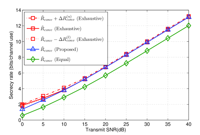
Figure 2: The achievable secrecy rate $\tilde{R}_{\rm conv}$ with different power allocations versus SNR.

In this section, we verify numerically our theoretical claims and compare the achievable secrecy rates of different training and power allocation schemes. Unless mentioned otherwise, the number of antennas at the source is $n_{t}=16$, the coherence interval is $T=480$, the forward training length is $T_{f}=16$, and the reverse training length is $T_{r}=1$ (when considering the DCE scheme). The transmit SNR is defined as $P/\sigma^{2}$ and the channel variances are $\sigma_{h}^{2}=\sigma_{g}^{2}=0.5$.

In Fig. 2, we show the approximate achievable secrecy rate $\tilde{R}_{\rm conv}(\hat{\mathcal{P}}^{*}_{\rm conv})$ of the conventional training case with $\hat{\mathcal{P}}^{*}_{\rm conv}$ being the proposed power allocation given in (30) (labeled as “$\tilde{R}_{\rm conv}\text{ (Proposed)}$”) and compare it with the maximum value $\max\limits_{\mathcal{P}}\tilde{R}_{\rm conv}(\mathcal{P})$ obtained via exhaustive search (i.e., “$\tilde{R}_{\rm conv}\text{ (Exhaustive)}$”). We can see that the approximate solution given in (30) is indeed near optimal at high SNR and yields about $4$ dB improvement over the case with equal power allocation among all components (i.e., “$\tilde{R}_{\rm conv}\text{ (Equal)}$”). Moreover, by comparing $\tilde{R}_{\rm conv}(\hat{\mathcal{P}}^{*}_{\rm conv})$ with the optimized upper and lower bounds $\max\limits_{\mathcal{P}}\{\tilde{R}_{\rm conv}(\mathcal{P})+\Delta R_{\rm conv}^{(u)}(\mathcal{P})\}$ and $\max\limits_{\mathcal{P}}\{\tilde{R}_{\rm conv}(\mathcal{P})-\Delta R_{\rm conv}^{(l)}(\mathcal{P})\}$, respectively, (i.e., “$\tilde{R}_{\rm conv}+\Delta R_{\rm conv}^{(u)}\text{ (Exhaustive)}$” and “$\tilde{R}_{\rm conv}-\Delta R_{\rm conv}^{(l)}\text{ (Exhaustive)}$”), we can also see that the approximate secrecy rate expression $\tilde{R}_{\rm conv}(\hat{\mathcal{P}}^{*}_{\rm conv})$ indeed closely approximates the maximum achievable secrecy rate $R_{\rm conv}(\mathcal{P}^{*}_{\rm conv})$ (i.e., Theorem 2), where $\mathcal{P}^{*}_{\rm conv}$ is the power allocation that maximizes $R_{\rm conv}$, since $\max\limits_{\mathcal{P}}\{\tilde{R}_{\rm conv}(\mathcal{P})-\Delta R_{\rm conv}^{(l)}(\mathcal{P})\}\leq R_{\rm conv}(\mathcal{P}^{*}_{\rm conv})\leq\max\limits_{\mathcal{P}}\{\tilde{R}_{\rm conv}(\mathcal{P})+\Delta R_{\rm conv}^{(u)}(\mathcal{P})\}$ and $\tilde{R}_{\rm conv}(\hat{\mathcal{P}}^{*}_{\rm conv})\approx\max\limits_{\mathcal{P}}\{\tilde{R}_{\rm conv}(\mathcal{P})-\Delta R_{\rm conv}^{(l)}(\mathcal{P})\}\approx\max\limits_{\mathcal{P}}\{\tilde{R}_{\rm conv}(\mathcal{P})+\Delta R_{\rm conv}^{(u)}(\mathcal{P})\}$ at high SNR, as shown in Fig. 2.

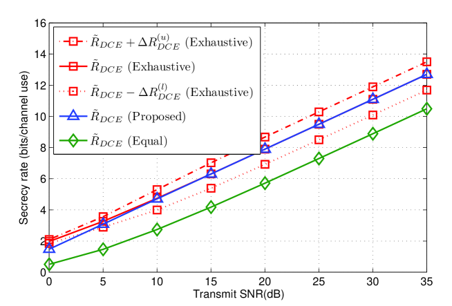
Figure 3: The achievable secrecy rate $\tilde{R}_{\rm DCE}$ with different power allocations versus SNR.

In Fig. 3, we show the approximate achievable secrecy rate $\tilde{R}_{\rm DCE}(\hat{\mathcal{P}}^{*}_{\rm DCE})$ of the DCE training case with $\hat{\mathcal{P}}^{*}_{\rm DCE}$ being the proposed solution obtained by Algorithm 1 (i.e. “$\tilde{R}_{\rm DCE}\text{ (Proposed)}$”) and compare it with the maximum value $\max\limits_{\mathcal{P}}\tilde{R}_{\rm DCE}(\mathcal{P})$ obtained via exhaustive search (i.e., “$\tilde{R}_{\rm DCE}\text{ (Exhaustive)}$”). Again, the secrecy rate obtained with the proposed solution rapidly converges towards the maximum value obtained via exhaustive search as the transmit SNR increases. A $7$ dB improvement is also observed when compared to the case with equal power allocation. Moreover, since the optimized upper and lower bounds $\max\limits_{\mathcal{P}}\{\tilde{R}_{\rm DCE}(\mathcal{P})+\Delta R_{\rm DCE}^{(u)}(\mathcal{P})\}$ and $\max\limits_{\mathcal{P}}\{\tilde{R}_{\rm DCE}(\mathcal{P})-\Delta R_{\rm DCE}^{(l)}(\mathcal{P})\}$ maintains a constant difference as the transmit SNR increases and, by Fig. 3, $\tilde{R}_{\rm DCE}(\hat{\mathcal{P}}^{*}_{\rm DCE})$ maintains between the two bounds, it follows that the difference between the approximate and the actual rates, i.e., $\tilde{R}_{\rm DCE}(\hat{\mathcal{P}}^{*}_{\rm DCE})-R_{\rm DCE}(\mathcal{P}^{*}_{\rm DCE})$, where $\mathcal{P}^{*}_{\rm DCE}$ is the power allocation that maximizes $R_{\rm DCE}$, becomes negligible compared to $R_{\rm DCE}(\mathcal{P}_{\rm DCE}^{*})$.

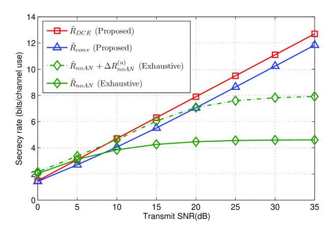
Figure 4: The achievable secrecy rate with different schemes versus SNR.

In Fig. 4, we compare the (approximate) achievable secrecy rate of different transmission schemes, namely, the case with conventional training (i.e., the case where AN is utilized only in the data transmission phase), the case with DCE training, and the case where no AN is used in either training or data transmission. Recall that $T_{d}=T-T_{f}-T_{r}$ where $T_{r}=1$ in the case with DCE training and is $0$ otherwise. We can observe that DCE training yields the best performance even though an additional channel use is required for reverse training. Moreover, we can see that, when AN is not used in either training and data transmission, the achievable secrecy rate becomes bounded as the transmit SNR increases, regardless of whether we are looking at $\tilde{R}_{\rm noAN}$ or the upper bound $\tilde{R}_{\rm noAN}+\Delta R_{\rm noAN}^{(u)}$. This indicates that the use of AN is critical to achieve good secrecy rate performance in the high SNR regime.

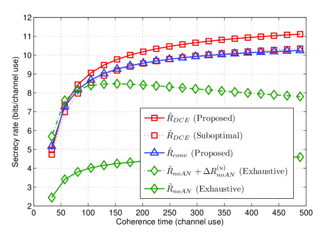
Figure 5: The achievable secrecy rate with different schemes versus coherence time.

In Fig. 5, we verify the effect of coherence time on the achievable secrecy rate of the different schemes. Here, the transmit SNR is fixed at $30$ dB. The DCE scheme with suboptimal power allocation refers to the power allocation used to prove the sufficient condition in Corollary 4. The suboptimal solution performs significantly worse than the proposed solution, but was sufficient to yield the condition in Corollary 4. In fact, with the proposed power allocation, DCE is able to outperform conventional training with a coherence time of only $70$, which is considerably smaller than the value $250$ required by the suboptimal power allocation. Yet, the latter is still smaller than the value $358.25$ predicted by Corollary 4, where the result is more conservative. Moreover, by comparing between “$\tilde{R}_{\rm DCE}$ (Proposed)” and “$\tilde{R}_{\rm conv}$ (Proposed)”, we can also see that the advantage of utilizing AN in the training phase increases as the coherence time increases. This is because, by applying AN in the training phase, we can allocate less energy to AN in the data transmission phase and, thus, more energy to the actual message-bearing signal.

VIII Conclusion

In this paper, we examined the impact of both conventional and AN-assisted training on the achievable secrecy rate of the AN-assisted secrecy beamforming scheme. Bounds on the achievable secrecy rate were first derived and then utilized to obtain a closed-form approximation that is shown to be asymptotically tight at high SNR. The approximate expression was then adopted as the objective function to determine the power allocation between pilot signals, data signals, and AN in both training and data transmission phases. An asymptotically optimal closed-form solution was obtained for the case with conventional training whereas a successive convex approximation approach was proposed for the case with DCE training. Furthermore, in the low SNR regime, we showed that AN provides no gains in secrecy rate and, thus, is not needed in either training or data transmission. Numerical simulations were provided to verify the tightness of the bounds and the advantages of DCE over conventional training.

Appendix A Proof of Theorem 1

Here, we first derive upper and lower bounds of $I(\mathbf{s}_{d};\mathbf{y}_{d}|\hat{\mathbf{h}})$ and $I(\mathbf{s}_{d};\mathbf{z}_{d}|\hat{\mathbf{h}},\hat{\mathbf{g}})$, and apply them directly to obtain the desired bounds for $R$, which is the difference of the two quantities. The derivations of the upper and lower bounds are shown only for $I(\mathbf{s}_{d};\mathbf{y}_{d}|\hat{\mathbf{h}})$ whereas that of $I(\mathbf{s}_{d};\mathbf{z}_{d}|\hat{\mathbf{h}},\hat{\mathbf{g}})$ can be obtained similarly.

A-A Lower Bound of $I(\mathbf{s}_{d};\mathbf{y}_{d}|\hat{\mathbf{h}})$

To derive the lower bound of $I(\mathbf{s}_{d};\mathbf{y}_{d}|\hat{\mathbf{h}})$, let us write

$$I(\mathbf{s}_{d};\mathbf{y}_{d}|\hat{\mathbf{h}})=h(\mathbf{s}_{d}|\hat{\mathbf{h}})-h(\mathbf{s}_{d}|\mathbf{y}_{d},\hat{\mathbf{h}}),$$ (50)

where $h(\mathbf{s}_{d}|\hat{\mathbf{h}})=h(\mathbf{s}_{d})=T_{d}\log(\pi e)$ and $h(\mathbf{s}_{d}|\mathbf{y}_{d},\hat{\mathbf{h}})\leq\mathbb{E}_{\hat{\mathbf{h}},\mathbf{y}_{d}}\left[\log\left((\pi e)^{T_{d}}\left|\mathbf{C}_{\mathbf{s}_{d}|\mathbf{y}_{d},\hat{\mathbf{h}}}\right|\right)\right]$ since Gaussian maximizes entropy. Here, $\mathbf{C}_{\mathbf{a}|\mathbf{b}}$ represents the covariance matrix of $\mathbf{a}$ given $\mathbf{b}$, and $|\mathbf{A}|$ represents the determinant of $\mathbf{A}$. Moreover, for any estimate $\hat{\mathbf{s}}_{d}$ of $\mathbf{s}_{d}$ given $\mathbf{y}_{d}$ and $\hat{\mathbf{h}}$, we have $\mathbf{C}_{\mathbf{s}_{d}|\mathbf{y}_{d},\hat{\mathbf{h}}}\preccurlyeq\mathbb{E}_{\mathbf{s}_{d}|\mathbf{y}_{d},\hat{\mathbf{h}}}\left[(\mathbf{s}_{d}-\hat{\mathbf{s}}_{d})(\mathbf{s}_{d}-\hat{\mathbf{s}}_{d})^{{\dagger}}\right]$, where $A\preccurlyeq B$ denotes that $A-B$ is semi-negative definite, and thus $\left|\mathbf{C}_{\mathbf{s}_{d}|\mathbf{y}_{d},\hat{\mathbf{h}}}\right|\leq\left|\mathbb{E}_{\mathbf{s}_{d}|\mathbf{y}_{d},\hat{\mathbf{h}}}\left[(\mathbf{s}_{d}-\hat{\mathbf{s}}_{d})(\mathbf{s}_{d}-\hat{\mathbf{s}}_{d})^{{\dagger}}\right]\right|$. Therefore, for $\hat{\mathbf{s}}_{d}^{L}=\mathbf{C}_{\mathbf{s}_{d}\mathbf{y}_{d}|\hat{\mathbf{h}}}\mathbf{C}_{\mathbf{y}_{d}|\hat{\mathbf{h}}}^{-1}\mathbf{y}_{d}$ (i.e., the LMMSE of $\mathbf{s}_{d}$ given $\mathbf{y}_{d}$ while assuming that $\hat{\mathbf{h}}$ is known), we have

$$\mathbb{E}_{\hat{\mathbf{h}},\mathbf{y}_{d}}\!\left[\log\left((\pi e)^{T_{d}}\left|\mathbf{C}_{\mathbf{s}_{d}|\mathbf{y}_{d},\hat{\mathbf{h}}}\right|\right)\right]$$

$$\leq\mathbb{E}_{\hat{\mathbf{h}}}\left[\mathbb{E}_{\mathbf{y}_{d}|\hat{\mathbf{h}}}\left[\log\left((\pi e)^{T_{d}}\left|\mathbb{E}_{\mathbf{s}_{d}|\mathbf{y}_{d},\hat{\mathbf{h}}}\left[(\mathbf{s}_{d}-\hat{\mathbf{s}}_{d}^{L})(\mathbf{s}_{d}-\hat{\mathbf{s}}_{d}^{L})^{{\dagger}}\right]\right|\right)\right]\right]$$ (51)

$$\leq\mathbb{E}_{\hat{\mathbf{h}}}\left[\log\left((\pi e)^{T_{d}}\left|\mathbf{C}_{\mathbf{s}_{d}|\hat{\mathbf{h}}}-\mathbf{C}_{\mathbf{s}_{d}\mathbf{y}_{d}|\hat{\mathbf{h}}}\mathbf{C}_{\mathbf{y}_{d}|\hat{\mathbf{h}}}^{-1}\mathbf{C}_{\mathbf{y}_{d}\mathbf{s}_{d}|\hat{\mathbf{h}}}\right|\right)\right]$$ (52)

$$=\mathbb{E}_{\hat{\mathbf{h}}}\!\left[\log\left((\pi e)^{T_{d}}\left|\mathbf{I}_{T_{d}}-\frac{P_{d}\|\hat{\mathbf{h}}\|^{2}}{P_{d}\|\hat{\mathbf{h}}\|^{2}+P_{d}\sigma^{2}_{\Delta h}+P_{a}\sigma^{2}_{\Delta h}+{\sigma^{2}}}\mathbf{I}_{T_{d}}\right|\right)\right],$$ (53)

where the last inequality follows from Jensen’s inequality. Hence, by combining (50) and (53), we have

$$I(\mathbf{s}_{d};\mathbf{y}_{d}|\hat{\mathbf{h}})\geq T_{d}\mathbb{E}_{\hat{\mathbf{h}}}\left[\log\left(1+\frac{P_{d}\|\mathbf{\hat{h}}\|^{2}}{P_{d}\sigma^{2}_{\Delta h}+P_{a}\sigma^{2}_{\Delta h}+{\sigma^{2}}}\right)\right].$$ (54)

A-B Upper Bound of $I(\mathbf{s}_{d};\mathbf{y}_{d}|\hat{\mathbf{h}})$

To obtain the upper bound, we instead write

$$I(\mathbf{s}_{d};\mathbf{y}_{d}|\hat{\mathbf{h}})=h(\mathbf{y}_{d}|\hat{\mathbf{h}})-h(\mathbf{y}_{d}|\mathbf{s}_{d},\hat{\mathbf{h}})$$ (55)

where $h(\mathbf{y}_{d}|\hat{\mathbf{h}})\leq\mathbb{E}_{\hat{\mathbf{h}}}\left[\log\left((\pi e)^{T_{d}}\left|\mathbf{C}_{\mathbf{y}_{d}|\hat{\mathbf{h}}}\right|\right)\right]$ since Gaussian maximizes entropy and $h(\mathbf{y}_{d}|\mathbf{s}_{d},\hat{\mathbf{h}})=h(\sqrt{P_{d}}\,\mathbf{s}_{d}\mathbf{\frac{\hat{h}^{{\dagger}}}{\|\hat{h}\|}}\mathbf{\Delta h}+\mathbf{A}_{d}\mathbf{N}_{\hat{\mathbf{h}}}\mathbf{\Delta h}+\mathbf{v}_{d}|\mathbf{s}_{d},\hat{\mathbf{h}})$ by (9). Notice that $h(\mathbf{y}_{d}|\mathbf{s}_{d},\hat{\mathbf{h}})$ is difficult to evaluate since $\mathbf{A}_{d}\mathbf{N}_{\hat{\mathbf{h}}}\mathbf{\Delta h}$ is non-Gaussian. Hence, we resort to the following large $n_{t}$ analysis.

Lemma 1

Let $\mathbf{A}$ be a $t\times(n-1)$ matrix with entries being i.i.d. ${\cal CN}\left(0,\frac{P}{n-1}\right)$, $\mathbf{N}$ be a $(n-1)\times n$ semi-unitary matrix such that $\mathbf{N}\mathbf{N}^{\dagger}=\mathbf{I}$, and $\Delta\mathbf{h}$ be an $n\times 1$ vector with entries being i.i.d. ${\cal CN}(0,\sigma_{\Delta h}^{2})$. Then, $\mathbf{A}\mathbf{N}\Delta\mathbf{h}$ converges in distribution to a Gaussian vector with entries being i.i.d. ${\cal CN}(0,P\sigma^{2}_{\Delta h})$ as $n\rightarrow\infty$.

Proof.

Let $\{\mathbf{N}\}_{i,j}$ denote the $(i,j)$-th entry of matrix $\mathbf{N}$ and let $\Delta\mathbf{h}_{j}$ denote the $j$-entry of vector $\Delta\mathbf{h}$. Then, we can define the vector ${\bf b}\triangleq\mathbf{N}\Delta\mathbf{h}$ whose $i$-th entry can be written as ${\bf b}_{i}=\sum_{j}\{\mathbf{N}\}_{i,j}\Delta\mathbf{h}_{j}$. Note that $\bf b$ is a Gaussian vector with entries that are i.i.d. with mean $0$ and variance $\sigma_{\Delta h}^{2}$ since, regardless of the value of $\mathbf{N}$, $\mathbb{E}[{\bf b}_{i}{\bf b}_{k}^{*}|\mathbf{N}]=\sum_{j}\sum_{\ell}\{\mathbf{N}\}_{i,j}\{\mathbf{N}\}_{k,\ell}^{*}\mathbb{E}\left[\Delta\mathbf{h}_{j}\Delta\mathbf{h}_{\ell}^{*}\right]=\sigma_{\Delta h}^{2}$, for $i=k$, and $0$, otherwise. Then, it follows by central limit theorem that the $i$-th entry of vector $\mathbf{A}\mathbf{N}\Delta\mathbf{h}=\mathbf{A}{\bf b}$, i.e., $\sum_{j}\{\mathbf{A}\}_{i,j}{\bf b}_{j}=\frac{1}{\sqrt{(n-1)}}\sum_{j}\{\overline{\mathbf{A}}\}_{i,j}{\bf b}_{j}$ where $\{\overline{\mathbf{A}}\}_{i,j}\triangleq\sqrt{n-1}\{\mathbf{A}\}_{i,j}\sim{\cal CN}\left(0,P\right)$, converges in distribution to a Gaussian random variable with mean $0$ and variance $P\sigma^{2}_{\Delta h}$, as $n\rightarrow\infty$. Moreover, since $\sum_{j}\sum_{\ell}\mathbb{E}[\{\mathbf{A}\}_{i,j}{\bf b}_{j}\{\mathbf{A}\}_{k,\ell}{\bf b}_{\ell}]=0$ for $i\neq k$ (i.e., the entries of $\mathbf{A}{\bf b}$ are uncorrelated), it follows that $\mathbf{A}{\bf b}$ converges in distribution to a Gaussian vector with entries that are i.i.d. ${\cal CN}(0,P\sigma^{2}_{\Delta h})$, as $n\rightarrow\infty$. ∎

By Lemma 1 (with $n=n_{t}$, $t=T_{d}$, and $P=P_{a}$), we know that $\mathbf{A}_{d}\mathbf{N}_{\hat{\mathbf{h}}}\mathbf{\Delta h}$ is asymptotically Gaussian as $n_{t}\rightarrow\infty$ if $\Delta\mathbf{h}$ is Gaussian as well. Hence, for $n_{t}$ sufficiently large, we have

$$I(\mathbf{s}_{d};\mathbf{y}_{d}|\hat{\mathbf{h}}) \leq\mathbb{E}_{\hat{\mathbf{h}}}\left[\log\left((\pi e)^{T_{d}}\left|\mathbf{C}_{\mathbf{y}_{d}|\hat{\mathbf{h}}}\right|\right)\right]-\mathbb{E}_{\hat{\mathbf{h}}}\left[\log\left((\pi e)^{T_{d}}\left|\mathbf{C}_{\mathbf{y}_{d}|\mathbf{s}_{d},\hat{\mathbf{h}}}\right|\right)\right]$$ (56)

$$=\mathbb{E}_{\hat{\mathbf{h}}}\left[\log\frac{\left|\left(\!P_{d}\|\mathbf{\hat{h}}\|^{2}\!+\!P_{d}\sigma^{2}_{\Delta h}\!+\!P_{a}\sigma^{2}_{\Delta h}\!+\!{\sigma^{2}}\!\right)\mathbf{I}_{T_{d}}\right|}{\left|P_{d}\sigma^{2}_{\Delta h}\mathbf{s}_{d}\mathbf{s}_{d}^{{\dagger}}\!+\!(P_{a}\sigma^{2}_{\Delta h}\!+\!{\sigma^{2}})\mathbf{I}_{T_{d}}\right|}\!\right]$$ (57)

$$=\mathbb{E}_{\hat{\mathbf{h}}}\left[\log\frac{\left(\!P_{d}\|\mathbf{\hat{h}}\|^{2}\!+\!P_{d}\sigma^{2}_{\Delta h}\!+\!P_{a}\sigma^{2}_{\Delta h}\!+\!{\sigma^{2}}\!\right)^{T_{d}}(P_{d}\sigma^{2}_{\Delta h}\!+\!P_{a}\sigma^{2}_{\Delta h}+\!{\sigma^{2}})^{T_{d}}}{(P_{d}\sigma^{2}_{\Delta h}\!+\!P_{a}\sigma^{2}_{\Delta h}+\!{\sigma^{2}})^{T_{d}}\left(\left(P_{a}\sigma^{2}_{\Delta h}\!+\!{\sigma^{2}}\right)^{T_{d}}\left|\frac{P_{d}\sigma^{2}_{\Delta h}\mathbf{s}_{d}\mathbf{s}_{d}^{{\dagger}}}{P_{a}\sigma^{2}_{\Delta h}\!+\!{\sigma^{2}}}\!+\!\mathbf{I}_{T_{d}}\right|\right)}\!\right]$$ (58)

$$=T_{d}\mathbb{E}_{\hat{\mathbf{h}}}\left[\log\left(1+\frac{P_{d}\|\mathbf{\hat{h}}\|^{2}}{P_{d}\sigma^{2}_{\Delta h}+P_{a}\sigma^{2}_{\Delta h}+{\sigma^{2}}}\right)\right]+T\Delta R^{(u)}.$$ (59)

Similarly, it also holds, for $\Delta\mathbf{g}$ Gaussian and $n_{t}$ sufficiently large, that

$$T_{d}\mathbb{E}\left[\log\left(1+\frac{P_{d}\frac{\mathbf{\hat{g}^{{\dagger}}\hat{h}\hat{h}^{{\dagger}}\hat{g}}}{\|\mathbf{\hat{h}}\|^{2}}}{P_{d}\sigma^{2}_{\Delta g}+P_{a}\frac{\|\mathbf{N}_{\hat{\mathbf{h}}}\mathbf{\hat{g}}\|^{2}}{n_{t}-1}+P_{a}\sigma^{2}_{\Delta g}+\sigma^{2}}\right)\right]\leq I(\mathbf{s}_{d};\mathbf{z}_{d}|\hat{\mathbf{h}},\hat{\mathbf{g}})$$

$$\hskip 28.45274pt\leq T_{d}\mathbb{E}\left[\log\left(1+\frac{P_{d}\frac{\mathbf{\hat{g}^{{\dagger}}\hat{h}\hat{h}^{{\dagger}}\hat{g}}}{\|\mathbf{\hat{h}}\|^{2}}}{P_{d}\sigma^{2}_{\Delta g}+P_{a}\frac{\|\mathbf{N}_{\hat{\mathbf{h}}}\mathbf{\hat{g}}\|^{2}}{n_{t}-1}+P_{a}\sigma^{2}_{\Delta g}+\sigma^{2}}\right)\right]+T\Delta R^{(l)}$$ (60)

By combining the above bounds for $I(\mathbf{s}_{d};\mathbf{y}_{d}|\hat{\mathbf{h}})$ and $I(\mathbf{s}_{d};\mathbf{z}_{d}|\hat{\mathbf{h}},\hat{\mathbf{g}})$, we obtain the bounds of the achievable secrecy rate in Theorem 1.

Appendix B Proof of Theorem 2 and Corollary 2

B-A Proof of Theorem 2

Let us consider the linear power allocation $\mathcal{P}_{l}\triangleq(P_{f,l},P_{d,l},P_{a,l})=(\alpha_{f}P,\beta_{d}P,\beta_{a}P)$ for some positive constants $\alpha_{f}$, $\beta_{d}$, and $\beta_{a}$ such that $\alpha_{f}PT_{f}+\beta_{d}PT_{d}+\beta_{a}PT_{d}\leq PT$. Then, by Theorem 1, it follows that

$$\tilde{R}_{\rm conv}(\mathcal{P}_{l})\!-\!\Delta R^{(l)}_{\rm conv}(\mathcal{P}_{l})\!\leq\!R_{\rm conv}(\mathcal{P}^{*})\!\leq\!\tilde{R}_{\rm conv}(\mathcal{P}^{*})\!+\!\Delta R^{(u)}_{\rm conv}(\mathcal{P}^{*}).$$ (61)

Hence, to obtain Theorem 2, it is sufficient to show that $\tilde{R}_{\rm conv}(\mathcal{P}_{l})-\Delta R^{(l)}_{\rm conv}(\mathcal{P}_{l})\doteq\tilde{R}_{\rm conv}(\mathcal{P}^{*})+\Delta R^{(u)}_{\rm conv}(\mathcal{P}^{*})$, i.e., $R_{\rm conv}(\mathcal{P}^{*})\doteq\tilde{R}_{\rm conv}(\mathcal{P}^{*})+\Delta R^{(u)}_{\rm conv}(\mathcal{P}^{*})$, and $\lim\limits_{P\rightarrow\infty}\Delta R^{(u)}_{\rm conv}(\mathcal{P}^{*})/R_{\rm conv}(\mathcal{P}^{*})=0$.

Specifically, by substituting $\mathcal{P}_{l}$ into (19) and (20), we can express the channel estimation error variances as $\sigma^{2}_{\Delta h}=\frac{\sigma_{h}^{2}\sigma^{2}}{\alpha_{f}P\sigma_{h}^{2}+\sigma^{2}}=\frac{\sigma^{2}}{\alpha_{f}P}+o\left(\frac{1}{P}\right)$ and $\sigma^{2}_{\Delta g}=\frac{\sigma_{g}^{2}\sigma^{2}}{\alpha_{f}P\sigma_{g}^{2}+\sigma^{2}}=\frac{\sigma^{2}}{\alpha_{f}P}+o\left(\frac{1}{P}\right)$. Then, it follows that

$$\tilde{R}_{\rm conv}(\mathcal{P}_{l})\!= \frac{T_{d}}{T}\mathbb{E}\left\{\log\left[1+\frac{\beta_{d}P(\sigma_{h}^{2}+o(1))\|\mathbf{\overline{h}}\|^{2}}{(\beta_{d}+\beta_{a})P\left(\frac{\sigma^{2}}{\alpha_{f}P}\!+\!o\left(\frac{1}{P}\right)\right)\!+\!\sigma^{2}}\right]\right\}$$

$$~{}-\frac{T_{d}}{T}\mathbb{E}\!\left\{\log\!\left[\!1\!+\!\frac{\beta_{d}P(\sigma_{g}^{2}\!+\!o(1))\frac{\mathbf{\overline{g}^{{\dagger}}\overline{h}\overline{h}^{{\dagger}}\overline{g}}}{\|\mathbf{\overline{h}}\|^{2}}}{(\beta_{d}\!+\!\beta_{a})P\left(\frac{\sigma^{2}}{\alpha_{f}P}\!+\!o\left(\frac{1}{P}\right)\right)\!+\!\beta_{a}P(\sigma_{g}^{2}+o(1))\frac{\|\mathbf{N}_{\hat{\mathbf{h}}}\mathbf{\overline{g}}\|^{2}}{n_{t}-1}\!+\!\sigma^{2}}\!\right]\!\right\}$$ (62)

$$= \frac{T_{d}}{T}\mathbb{E}\!\left[\log\frac{\beta_{d}P\sigma_{h}^{2}\|\mathbf{\overline{h}}\|^{2}\!+\!o(P)}{\frac{\sigma^{2}(\beta_{d}+\beta_{a})}{\alpha_{f}}\!+\!\sigma^{2}\!+\!o(1)}\!\right]\!-\!\frac{T_{d}}{T}\mathbb{E}\left[\log\!\left(\!1\!+\!\frac{\beta_{d}P\sigma_{g}^{2}\frac{\mathbf{\overline{g}^{{\dagger}}\overline{h}\overline{h}^{{\dagger}}\overline{g}}}{\|\mathbf{\overline{h}}\|^{2}}\!+\!o(P)}{\beta_{a}P\sigma_{g}^{2}\frac{\|\mathbf{N}_{\hat{\mathbf{h}}}\mathbf{\overline{g}}\|^{2}}{n_{t}-1}\!+\!o(P)}\!\right)\!\right]$$ (63)

$$= \frac{T_{d}}{T}\mathbb{E}\left[\log\frac{\beta_{d}P\sigma_{h}^{2}\|\mathbf{\overline{h}}\|^{2}}{\left(\frac{\beta_{d}+\beta_{a}}{\alpha_{f}}+1\right){\sigma^{2}}}\right]-\frac{T_{d}}{T}\mathbb{E}\left[\log\left(1+\frac{\beta_{d}\frac{\mathbf{\overline{g}^{{\dagger}}\overline{h}\overline{h}^{{\dagger}}\overline{g}}}{\|\mathbf{\overline{h}}\|^{2}}}{\beta_{a}\frac{\|\mathbf{N}_{\hat{\mathbf{h}}}\mathbf{\overline{g}}\|^{2}}{n_{t}-1}}\right)\right]+o(1)$$ (64)

$$= \frac{T_{d}}{T}\log P+c_{1}+o(1),$$ (65)

where

$$c_{1}\triangleq\frac{T_{d}}{T}\mathbb{E}\left[\log\frac{\beta_{d}\sigma_{h}^{2}\|\mathbf{\overline{h}}\|^{2}}{\left(\frac{\beta_{d}+\beta_{a}}{\alpha_{f}}+1\right){\sigma^{2}}}\right]-\frac{T_{d}}{T}\mathbb{E}\left[\log\left(1+\frac{\beta_{d}\frac{\mathbf{\overline{g}^{{\dagger}}\overline{h}\overline{h}^{{\dagger}}\overline{g}}}{\|\mathbf{\overline{h}}\|^{2}}}{\beta_{a}\frac{\|\mathbf{N}_{\hat{\mathbf{h}}}\mathbf{\overline{g}}\|^{2}}{n_{t}-1}}\right)\right]$$ (66)

is a finite constant that is independent of $P$, and

$$\!\!\!\!\Delta R^{(l)}_{\rm conv}(\mathcal{P}_{l})\!$$

$$= ~{}\frac{1}{T}\mathbb{E}\!\left\{\log\frac{\left[(\beta_{d}\!+\!\beta_{a})P\left(\frac{\sigma^{2}}{\alpha_{f}P}\!+\!o\left(\frac{1}{P}\right)\right)\!+\!\beta_{a}P\left(\sigma_{g}^{2}\!+\!o(1)\right)\frac{\|\mathbf{N}_{\hat{\mathbf{h}}}\mathbf{\overline{g}}\|^{2}}{n_{t}-1}\!+\!\sigma^{2}\!\right]^{T_{d}}}{\left[\beta_{a}P\left(\sigma_{g}^{2}\!+\!o(1)\right)\frac{\|\mathbf{N}_{\hat{\mathbf{h}}}\mathbf{\overline{g}}\|^{2}}{n_{t}-1}\!+\!\beta_{a}P\left(\frac{\sigma^{2}}{\alpha_{f}P}\!+\!o\left(\frac{1}{P}\right)\right)\!+\!\sigma^{2}\!\right]^{T_{d}-1}}\right\}$$

$$-\frac{1}{T}\mathbb{E}\!\left\{\log\!\left[(\beta_{d}\|\mathbf{s}_{d}\|^{2}\!+\!\beta_{a})P\left(\frac{\sigma^{2}}{\alpha_{f}P}\!+\!o\left(\frac{1}{P}\right)\right)\!+\!\beta_{a}P\!\left(\sigma_{g}^{2}\!+\!o(1)\right)\!\frac{\|\mathbf{N}_{\hat{\mathbf{h}}}\mathbf{\overline{g}}\|^{2}}{n_{t}\!-\!1}\!+\!\sigma^{2}\!\right]\!\right\}\!$$ (67)

$$= ~{}\frac{1}{T}\mathbb{E}\!\left[\log\frac{\left(\beta_{a}P\sigma_{g}^{2}\frac{\|\mathbf{N}_{\hat{\mathbf{h}}}\mathbf{\overline{g}}\|^{2}}{n_{t}-1}\!+\!o(P)\!\right)^{T_{d}}}{\left(\beta_{a}P\sigma_{g}^{2}\frac{\|\mathbf{N}_{\hat{\mathbf{h}}}\mathbf{\overline{g}}\|^{2}}{n_{t}-1}\!+\!o(P)\!\right)^{\!T_{d}-1}}\right]\!-\!\frac{1}{T}\mathbb{E}\!\left[\log\!\left(\!\beta_{a}P\sigma_{g}^{2}\frac{\|\mathbf{N}_{\hat{\mathbf{h}}}\mathbf{\overline{g}}\|^{2}}{n_{t}\!-\!1}\!+\!o(P)\!\right)\!\right]=o(1).$$ (68)

Hence,

$$\tilde{R}_{\rm conv}(\mathcal{P}_{l})-\Delta R^{(l)}_{\rm conv}(\mathcal{P}_{l})=\frac{T_{d}}{T}\log P+c_{1}+o(1).$$ (69)

Moreover, by (1) and (15), we can write

$$\tilde{R}_{\rm conv}(\mathcal{P}^{*})+\Delta R^{(u)}_{\rm conv}(\mathcal{P}^{*})$$

$$\overset{(a)}{\leq}\frac{T_{d}}{T}\mathbb{E}\!\left[\log\!\left(1\!+\!\frac{P_{d}^{*}(\sigma_{h}^{2}\!-\!\sigma^{2}_{\Delta h})\|\mathbf{\overline{h}}\|^{2}}{P_{d}^{*}\sigma^{2}_{\Delta h}\!+\!P_{a}^{*}\sigma^{2}_{\Delta h}\!+\!\sigma^{2}}\!\right)\!\right]$$

$$~{}~{}~{}~{}+\frac{1}{T}\log\left(P_{d}^{*}\sigma^{2}_{\Delta h}+P_{a}^{*}\sigma^{2}_{\Delta h}+\sigma^{2}\right)^{T_{d}}\!-\!\frac{1}{T}\mathbb{E}\left[\log\!\left(P_{d}^{*}\|\mathbf{s}_{d}\|^{2}\sigma^{2}_{\Delta h}\right)\right]$$ (70)

$$\overset{(b)}{\leq}\frac{T_{d}}{T}\mathbb{E}\!\left[\log\!\left(k^{\prime}P\left(2\sigma^{2}_{\Delta h}\!+\!1\!+\!(\sigma_{h}^{2}\!-\!\sigma^{2}_{\Delta h})\|\mathbf{\overline{h}}\|^{2}\right)\right)\right]-\frac{1}{T}\mathbb{E}\left[\log\!\left(P_{d}^{*}\|\mathbf{s}_{d}\|^{2}\sigma^{2}_{\Delta h}\right)\right]$$ (71)

$$=\frac{T_{d}}{T}\log P-\frac{1}{T}\log\left(P_{d}^{*}\sigma^{2}_{\Delta h}\right)+c_{2},$$ (72)

where $c_{2}\triangleq(1/T)\mathbb{E}\!\left[\log\!\left(\left(k^{\prime}\left(2\sigma^{2}_{\Delta h}\!+\!1\!+\!(\sigma_{h}^{2}\!-\!\sigma^{2}_{\Delta h})\|\mathbf{\overline{h}}\|^{2}\right)\right)^{T_{d}}/\|\mathbf{s}_{d}\|^{2}\right)\right]$ is a finite constant. The inequality in (a) follows by eliminating the negative term of $\tilde{R}_{\rm conv}(\mathcal{P}^{*})$ in (1) and by eliminating some positive parts in the denominator of the first term as well as in the second term of $\Delta R^{(u)}_{\rm conv}$ in (15); and (b) is obtained by upper-bounding $P_{d}$, $P_{a}$, and $\sigma^{2}$ by $k^{\prime}P$, where $k^{\prime}$ is chosen such that $k^{\prime}P\geq\max\{P_{d},P_{a},\sigma^{2}\}$. By (61), (69), and (72), it follows that $P_{d}^{*}\sigma_{\Delta h}^{2}=O(1)$ (since otherwise the upper bound in (72) would be smaller than the lower bound in (69)). This implies that $\Delta R^{(u)}_{\rm conv}(\mathcal{P}^{*})$ is a finite constant and, thus, we can write

$$\tilde{R}_{\rm conv}(\mathcal{P}^{*})+\Delta R^{(u)}_{\rm conv}(\mathcal{P}^{*}) \leq\frac{T_{d}}{T}\mathbb{E}\!\left[\log\left(1\!+\!P_{d}^{*}(\sigma_{h}^{2}\!-\!\sigma^{2}_{\Delta h})\|\mathbf{\overline{h}}\|^{2}\right)\!\right]+\Delta R^{(u)}_{\rm conv}(\mathcal{P}^{*})$$ (73)

$$\leq\frac{T_{d}}{T}\log P+c_{2}^{\prime}+o(1),$$ (74)

for some constant $c_{2}^{\prime}\triangleq\frac{T_{d}}{T}\mathbb{E}\left[\log k^{\prime}(\sigma_{h}^{2}-\sigma^{2}_{\Delta h}+1)\|\mathbf{\overline{h}}\|^{2}\right]+\Delta R^{(u)}_{\rm conv}(\mathcal{P}^{*})$. By combining (69) and (74), we obtain the desired result $\tilde{R}_{\rm conv}(\mathcal{P}_{l})-\Delta R^{(l)}_{\rm conv}(\mathcal{P}_{l})\doteq\tilde{R}_{\rm conv}(\mathcal{P}^{*})+\Delta R^{(u)}_{\rm conv}(\mathcal{P}^{*})$. Moreover, since $\Delta R^{(u)}_{\rm conv}(\mathcal{P}^{*})$ is finite, we have $\lim\limits_{P\rightarrow\infty}\Delta R^{(u)}_{\rm conv}(\mathcal{P}^{*})/R_{\rm conv}(\mathcal{P}^{*})\!=\!0$, which completes the proof.

B-B Proof of Corollary 2

The proof of the corollary relies on the fact that

$$\tilde{R}_{\rm conv}(\mathcal{P}_{l})-\Delta R^{(l)}_{\rm conv}(\mathcal{P}_{l})\leq\tilde{R}_{\rm conv}(\mathcal{P}^{*})+\Delta R^{(u)}_{\rm conv}(\mathcal{P}^{*})$$ (75)

for any linear power allocation $\mathcal{P}_{l}$.

Specifically, let us first consider the upper bound

$$R_{\rm conv}(\mathcal{P}^{*})\overset{(a)}{\leq} \frac{T_{d}}{T}\mathbb{E}\left[\log\left(1+P_{d}^{*}\sigma_{h}^{2}\|\mathbf{\overline{h}}\|^{2}/\sigma^{2}\right)\right]+\Delta R^{(u)}_{\rm conv}$$ (76)

$$\overset{(b)}{\leq} \frac{T_{d}}{T}\log\left(1+P_{d}^{*}\sigma_{h}^{2}/\sigma^{2}\right)+\Delta R^{(u)}_{\rm conv},$$ (77)

where (a) is obtained by eliminating the negative terms in $\tilde{R}_{\rm conv}(\mathcal{P})$ and by lower-bounding the denominator of the first term by $\sigma^{2}$, and (b) follows from Jensen’s inequality. By the argument below (72), we know that $P_{d}^{*}\sigma_{\Delta h}^{2}=O(1)$, and thus, $R^{(u)}_{\rm conv}(\mathcal{P}^{*})=O(1)$. Then, together with (75) and (69), we have $\frac{T_{d}}{T}\log\left(1+P_{d}^{*}\sigma_{h}^{2}/\sigma^{2}\right)+O(1)\geq\frac{T_{d}}{T}\log P+c_{1}+o(1)$, which implies that $P_{d}^{*}(P)=\Omega(P)$. Moreover, since $P_{d}^{*}\sigma_{\Delta h}^{2}=P_{d}^{*}\sigma_{h}^{2}\sigma^{2}/(P_{f}^{*}\sigma_{h}^{2}+\sigma^{2})=O(1)$, it also follows that $P_{f}^{*}(P)=\Omega(P_{d}^{*}(P))=\Omega(P)$. Furthermore, since $\sigma_{\Delta g}^{2}/\sigma_{\Delta h}^{2}=\frac{(P_{f}^{*}\sigma_{h}^{2}+\sigma^{2})/\sigma_{h}^{2}}{(P_{f}^{*}\sigma_{g}^{2}+\sigma^{2})/\sigma_{g}^{2}}=O(1)$, we know that $P_{d}\sigma_{\Delta g}^{2}=(P_{d}\sigma_{\Delta h}^{2})(\sigma_{\Delta g}^{2}/\sigma_{\Delta h}^{2})=O(1)$. Therefore, the achievable secrecy rate can be upper-bounded as

$$R_{\rm conv}\! \leq\tilde{R}_{\rm conv}+\Delta R^{(u)}_{\rm conv}$$ (78)

$$\leq\frac{T_{d}}{T}\mathbb{E}\left[\log\left(1+P_{d}^{*}\sigma_{h}^{2}\|\mathbf{\overline{h}}\|^{2}/\sigma^{2}\right)\right]$$

$$~{}~{}-\frac{T_{d}}{T}\mathbb{E}\!\left[\log\!\left(\!1\!+\!\frac{P_{d}^{*}(\sigma_{g}^{2}\!-\!\sigma^{2}_{\Delta g})\frac{\mathbf{\overline{g}^{{\dagger}}\overline{h}\overline{h}^{{\dagger}}\overline{g}}}{\|\mathbf{\overline{h}}\|^{2}}}{P_{d}^{*}\sigma^{2}_{\Delta g}\!+\!P_{a}^{*}(\sigma_{g}^{2}\!-\!\sigma^{2}_{\Delta g})\frac{\|\mathbf{N}_{\hat{\mathbf{h}}}\mathbf{\overline{g}}\|^{2}}{n_{t}\!-\!1}\!+\!P_{a}^{*}\sigma^{2}_{\Delta g}\!+\!\sigma^{2}}\right)\!\right]\!+\!\Delta R^{(u)}_{\rm conv}$$ (79)

$$\overset{(a)}{=}\frac{T_{d}}{T}\mathbb{E}\!\left[\log\!\left(1\!+\!P_{d}^{*}\sigma_{h}^{2}\|\mathbf{\overline{h}}\|^{2}/\sigma^{2}\right)\right]\!-\!\frac{T_{d}}{T}\mathbb{E}\!\left[\log\!\left(1\!+\!\frac{P_{d}^{*}\sigma_{g}^{2}\frac{\mathbf{\overline{g}^{{\dagger}}\overline{h}\overline{h}^{{\dagger}}\overline{g}}}{\|\mathbf{\overline{h}}\|^{2}}\!+\!o(P_{d}^{*})}{P_{a}^{*}\sigma_{g}^{2}\frac{\|\mathbf{N}_{\hat{\mathbf{h}}}\mathbf{\overline{g}}\|^{2}}{n_{t}\!-\!1}\!+\!o(P_{d}^{*})}\right)\right]\!+\!\Delta R^{(u)}_{\rm conv}$$ (80)

$$=\frac{T_{d}}{T}\log P_{d}^{*}-\frac{T_{d}}{T}\mathbb{E}\left[\log\left(1+\frac{P_{d}^{*}\frac{\mathbf{\overline{g}^{{\dagger}}\overline{h}\overline{h}^{{\dagger}}\overline{g}}}{\|\mathbf{\overline{h}}\|^{2}}+o(P^{*}_{d})}{P^{*}_{a}\frac{\|\mathbf{N}_{\hat{\mathbf{h}}}\mathbf{\overline{g}}\|^{2}}{n_{t}-1}+o(P^{*}_{d})}\right)\right]+c_{3}+o(1),$$ (81)

where $c_{3}=(T_{d}/T)\mathbb{E}\left[\log\left(\sigma_{h}^{2}\|\mathbf{\overline{h}}\|^{2}/\sigma^{2}\right)\right]+\Delta R^{(u)}_{\rm conv}$ is a finite constant and (a) holds since $P^{*}_{d}\sigma^{2}_{\Delta g}=O(1)$ and $P^{*}_{a}\sigma^{2}_{\Delta g}=O(1)$. From (81), we can observe that the second term is a negative finite constant only if $P^{*}_{a}(P)=\Omega(P_{d}^{*}(P))$ which implies that $P^{*}_{a}(P)=\Omega(P)$.

Appendix C Proof of (24) in Section IV

By the weak law of large numbers (WLLN), we know that $\|\mathbf{N}_{\hat{\mathbf{h}}}\mathbf{\overline{g}}\|^{2}/(n_{t}-1)\rightarrow 1$ in probability as $n_{t}\rightarrow\infty$. That is, for any $\epsilon>0$, we have $\Pr(A_{\epsilon})\rightarrow 1$ (and, thus, $\Pr(A_{\epsilon}^{c})\rightarrow 0$) as $n_{t}\rightarrow\infty$, where $A_{\epsilon}\triangleq\left\{\left|\frac{\|\mathbf{N}_{\hat{\mathbf{h}}}\mathbf{\overline{g}}\|^{2}}{n_{t}-1}-1\right|\leq\epsilon\right\}$. Therefore, for $n_{t}$ sufficiently large, the second expectation term in (23) can be written as

$$\!\!\!\!\mathbb{E}\left[\log\left(1+\frac{P^{*}_{d}\frac{\mathbf{\overline{g}^{{\dagger}}\overline{h}\overline{h}^{{\dagger}}\overline{g}}}{\|\mathbf{\overline{h}}\|^{2}}}{P^{*}_{a}\frac{\|\mathbf{N}_{\hat{\mathbf{h}}}\mathbf{\overline{g}}\|^{2}}{(n_{t}-1)}}\right)\Bigg{|}A_{\epsilon}\right]\Pr\left(A_{\epsilon}\right)+\mathbb{E}\left[\log\left(1+\frac{P^{*}_{d}\frac{\mathbf{\overline{g}^{{\dagger}}\overline{h}\overline{h}^{{\dagger}}\overline{g}}}{\|\mathbf{\overline{h}}\|^{2}}}{P^{*}_{a}\frac{\|\mathbf{N}_{\hat{\mathbf{h}}}\mathbf{\overline{g}}\|^{2}}{(n_{t}-1)}}\right)\Bigg{|}A_{\epsilon}^{c}\right]\Pr\left(A_{\epsilon}^{c}\right)$$

$$\leq ~{}\mathbb{E}\left[\log\left(1+\frac{P^{*}_{d}\frac{\mathbf{\overline{g}^{{\dagger}}\overline{h}\overline{h}^{{\dagger}}\overline{g}}}{\|\mathbf{\overline{h}}\|^{2}}}{P^{*}_{a}(1-\epsilon)}\right)\Bigg{|}A_{\epsilon}\right]\Pr\left(A_{\epsilon}\right)+\mathbb{E}\left[\log\left(1+\frac{P^{*}_{d}\frac{\mathbf{\overline{g}^{{\dagger}}\overline{h}\overline{h}^{{\dagger}}\overline{g}}}{\|\mathbf{\overline{h}}\|^{2}}}{P^{*}_{a}\frac{\|\mathbf{N}_{\hat{\mathbf{h}}}\mathbf{\overline{g}}\|^{2}}{(n_{t}-1)}}\right)\Bigg{|}A_{\epsilon}^{c}\right]\Pr\left(A_{\epsilon}^{c}\right)$$ (82)

$$\leq ~{}\mathbb{E}\left[\log\left(1+\frac{P^{*}_{d}\frac{\mathbf{\overline{g}^{{\dagger}}\overline{h}\overline{h}^{{\dagger}}\overline{g}}}{\|\mathbf{\overline{h}}\|^{2}}}{P^{*}_{a}(1-\epsilon)}\right)\right]+\epsilon_{n_{t}}.$$ (83)

where

$$\epsilon_{n_{t}}\triangleq\mathbb{E}\left[\log\left(1+\frac{P^{*}_{d}\frac{\mathbf{\overline{g}^{{\dagger}}\overline{h}\overline{h}^{{\dagger}}\overline{g}}}{\|\mathbf{\overline{h}}\|^{2}}}{P^{*}_{a}\frac{\|\mathbf{N}_{\hat{\mathbf{h}}}\mathbf{\overline{g}}\|^{2}}{(n_{t}-1)}}\right)\Bigg{|}A_{\epsilon}^{c}\right]\Pr\left(A_{\epsilon}^{c}\right).$$ (84)

Notice that $\epsilon_{n_{t}}\rightarrow 0$ as $n_{t}\rightarrow\infty$ since the expectation inside (84) is finite. Then, by applying Jensen’s inequality to the first term in (83), we have

$$\mathbb{E}\left[\log\left(1+\frac{P^{*}_{d}\frac{\mathbf{\overline{g}^{{\dagger}}\overline{h}\overline{h}^{{\dagger}}\overline{g}}}{\|\mathbf{\overline{h}}\|^{2}}}{P^{*}_{a}(1-\epsilon)}\right)\right]\leq\log\left(1+\frac{P^{*}_{d}}{P^{*}_{a}(1-\epsilon)}\right)\leq\log\left(\frac{P^{*}_{a}+P^{*}_{d}}{P^{*}_{a}(1-\epsilon)}\right)$$ (85)

Finally, by (23) and (85), we have

$$\tilde{R}_{\rm conv}\geq\frac{T_{d}}{T}\log\frac{\frac{P^{*}_{d}P^{*}_{a}}{P^{*}_{a}+P^{*}_{d}}}{\left(\frac{P^{*}_{d}+P^{*}_{a}}{P^{*}_{f}}+1\right)\sigma^{2}}+\frac{T_{d}}{T}\mathbb{E}\left[\log\left(\sigma_{h}^{2}\|\mathbf{\overline{h}}\|^{2}(1-\epsilon)\right)\right]+\frac{T_{d}}{T}\epsilon_{n_{t}}+o(1)$$ (86)

Appendix D Proof of Theorem 3 and Corollary 3

D-A Proof of Theorem 3

The proof of Theorem 3 is an extension of the proof of Theorem 2 in Appendix B and, thus, is explained more concisely in the following.

Specifically, let us also consider a linear power allocation $\mathcal{P}_{l}\triangleq(P_{r,l},P_{f,l},P_{f_{a},l},P_{d,l},P_{a,l})=(\alpha_{r}P,\alpha_{f}P,\alpha_{f_{a}}P,\beta_{d}P,\beta_{a}P)$, where $\alpha_{r},\alpha_{f},\alpha_{f_{a}},\beta_{d}$, and $\beta_{a}$ are positive constants chosen such that the total power constraint in (11) is satisfied. Similar to Appendix B, it is sufficient to show here that $\tilde{R}_{\rm DCE}(\mathcal{P}_{l})-\Delta R^{(l)}_{\rm DCE}(\mathcal{P}_{l})\doteq\tilde{R}_{\rm DCE}(\mathcal{P}^{*})+\Delta R^{(u)}_{\rm DCE}(\mathcal{P}^{*})$ and $\Delta R^{(u)}_{\rm DCE}(\mathcal{P}^{*})=O(1)$.

By substituting $\mathcal{P}_{l}$ into (6) and (7), we can write the channel estimation error variances as

$$\sigma^{2}_{\Delta h} =\frac{\sigma_{h}^{2}\left(P_{f_{a},l}\frac{\sigma_{h}^{2}\sigma^{2}}{\sigma^{2}+P_{r,l}\sigma_{h}^{2}}+\sigma^{2}\right)}{P_{f_{a},l}\frac{\sigma_{h}^{2}\sigma^{2}}{\sigma^{2}+P_{r,l}\sigma_{h}^{2}}+\sigma^{2}+P_{f,l}\sigma_{h}^{2}}=\frac{(\alpha_{f_{a}}+\alpha_{r})\sigma^{2}}{\alpha_{r}\alpha_{f}}P^{-1}+o(P^{-1}),$$ (87)

$$\sigma^{2}_{\Delta g} =\frac{P_{f_{a},l}\sigma^{4}_{g}+\sigma_{g}^{2}}{P_{f_{a},l}\sigma_{g}^{2}+\sigma^{2}+P_{f,l}\sigma_{g}^{2}}=\frac{\alpha_{f_{a}}\sigma_{g}^{2}}{\alpha_{f_{a}}+\alpha_{f}}+o(1).$$ (88)

Thus, we have

$$\tilde{R}_{\rm DCE}(\mathcal{P}_{l})= \frac{T_{d}}{T}\mathbb{E}\left[\log\left(1+\frac{\beta_{d}P(\sigma_{h}^{2}+o(1))\|\mathbf{\overline{h}}\|^{2}}{\left(\beta_{d}+\beta_{a}\right)\frac{(\alpha_{f_{a}}+\alpha_{r})\sigma^{2}}{\alpha_{r}\alpha_{f}}+o(1)+\sigma^{2}}\right)\right]$$

$$-\frac{T_{d}}{T}\mathbb{E}\!\left[\!\log\!\left(\!1\!+\!\frac{\beta_{d}P\left(\frac{\alpha_{f}\sigma_{g}^{2}}{\alpha_{f_{a}}+\alpha_{f}}+o(1)\right)\frac{\mathbf{\overline{g}^{{\dagger}}\overline{h}\overline{h}^{{\dagger}}\overline{g}}}{\|\mathbf{\overline{h}}\|^{2}}}{(\beta_{d}+\beta_{a})P\!\left(\frac{\alpha_{f_{a}}\sigma_{g}^{2}}{\alpha_{f_{a}}+\alpha_{f}}\!+\!o(1)\!\right)\!+\!\beta_{a}P\!\left(\frac{\alpha_{f}\sigma_{g}^{2}}{\alpha_{f_{a}}+\alpha_{f}}\!+\!o(1)\!\right)\!\frac{\|\mathbf{N}_{\hat{\mathbf{h}}}\mathbf{\overline{g}}\|^{2}}{n_{t}-1}\!+\!\sigma^{2}}\!\right)\!\right]$$ (89)

$$= \frac{T_{d}}{T}\mathbb{E}\left[\log\left(\frac{\beta_{d}P\sigma_{h}^{2}\|\mathbf{\overline{h}}\|^{2}}{\left(\beta_{d}+\beta_{a}\right)\frac{(\alpha_{f_{a}}+\alpha_{r})\sigma^{2}}{\alpha_{r}\alpha_{f}}+\sigma^{2}}\right)\right]$$

$$-\frac{T_{d}}{T}\mathbb{E}\left[\log\left(1+\frac{\beta_{d}\alpha_{f}\frac{\mathbf{\overline{g}^{{\dagger}}\overline{h}\overline{h}^{{\dagger}}\overline{g}}}{\|\mathbf{\overline{h}}\|^{2}}}{(\beta_{d}+\beta_{a})\alpha_{f_{a}}+\beta_{a}\alpha_{f}\frac{\|\mathbf{N}_{\hat{\mathbf{h}}}\mathbf{\overline{g}}\|^{2}}{n_{t}-1}}\right)\right]+o(1)$$ (90)

$$= \frac{T_{d}}{T}\log P+c_{4}+o(1).$$ (91)

where $c_{4}\triangleq\frac{T_{d}}{T}\mathbb{E}\left[\log\left(\frac{\beta_{d}\sigma_{h}^{2}\|\mathbf{\overline{h}}\|^{2}}{\left(\beta_{d}+\beta_{a}\right)\frac{(\alpha_{f_{a}}+\alpha_{r})\sigma^{2}}{\alpha_{r}\alpha_{f}}+\sigma^{2}}\right)\right]-\frac{T_{d}}{T}\mathbb{E}\left[\log\left(1+\frac{\beta_{d}\alpha_{f}\frac{\mathbf{\overline{g}^{{\dagger}}\overline{h}\overline{h}^{{\dagger}}\overline{g}}}{\|\mathbf{\overline{h}}\|^{2}}}{(\beta_{d}+\beta_{a})\alpha_{f_{a}}+\beta_{a}\alpha_{f}\frac{\|\mathbf{N}_{\hat{\mathbf{h}}}\mathbf{\overline{g}}\|^{2}}{n_{t}-1}}\right)\right]$. Moreover, by substituting $\mathcal{P}_{l}$ into (16), it can also be shown that $\Delta R^{(l)}_{\rm DCE}(\mathcal{P}_{l})=O(1)$. Hence, we have $\tilde{R}_{\rm DCE}(\mathcal{P}_{l})-\Delta R^{(l)}_{\rm DCE}(\mathcal{P}_{l})=\frac{T_{d}}{T}\log P+O(1).$

Furthermore, by following the derivations in (70)-(72), it can also be shown that $P_{d}^{*}\sigma_{\Delta h}^{2}=O(1)$ and, thus, $\tilde{R}_{\rm DCE}(\mathcal{P}^{*})+\Delta R^{(u)}_{\rm DCE}(\mathcal{P}^{*})\leq\frac{T_{d}}{T}\log P+O(1).$ Hence, it follows that $\tilde{R}_{\rm DCE}(\mathcal{P}_{l})-\Delta R^{(l)}_{\rm DCE}(\mathcal{P}_{l})\doteq\tilde{R}_{\rm DCE}(\mathcal{P}^{*})+\Delta R^{(u)}_{\rm DCE}(\mathcal{P}^{*})$.

D-B Proof of Corollary 3

The proofs of $P^{*}_{f}(P)=\Omega(P)$ and $P^{*}_{d}(P)=\Omega(P)$ are the same as those in Appendix B for the case with conventional training. Hence, we prove here that either $P_{fa}^{*}(P)=\Omega(P)$ or $P_{a}^{*}(P)=\Omega(P)$, and that $P_{r}^{*}(P)=\Omega(P_{fa}^{*}(P))$.

First, let us recall that

$$P_{d}^{*}\sigma^{2}_{\Delta h}=\frac{P_{d}^{*}\sigma_{h}^{2}\left(P_{f_{a}}^{*}\sigma_{\Delta h_{r}}^{2}+\sigma^{2}\right)}{P_{f}^{*}\sigma_{h}^{2}+P_{f_{a}}^{*}\sigma_{\Delta h_{r}}^{2}+\sigma^{2}}=O(1).$$ (92)

Due to the total power constraint, it holds that $P_{f}^{*}\sigma_{h}^{2}+P_{f_{a}}^{*}\sigma_{\Delta h_{r}}^{2}+\sigma^{2}=O(P)$. Therefore, together with the fact that $P^{*}_{d}(P)=\Omega(P)$, it follows that $P_{f_{a}}^{*}\sigma_{\Delta h_{r}}^{2}=O(1)$. Then, by (2), we have $P_{f_{a}}^{*}\sigma_{\Delta h_{r}}^{2}=\frac{P_{f_{a}}^{*}\sigma_{h}^{2}\sigma^{2}}{P_{r}^{*}\sigma_{h}^{2}+\sigma^{2}}=O(1)$, which implies that $P^{*}_{r}(P)=\Omega(P^{*}_{f_{a}}(P))$.

Finally, to show that $P^{*}_{f_{a}}(P)=\Omega(P)$ or $P^{*}_{a}(P)=\Omega(P)$, let us rewrite the upper bound of the achievable secrecy rate as follow:

$$\tilde{R}_{\rm DCE}+\Delta R^{(u)}_{\rm DCE}$$ (93)

$$\leq\frac{T_{d}}{T}\mathbb{E}\left[\log\left(1+P_{d}^{*}\sigma_{h}^{2}\|\mathbf{\overline{h}}\|^{2}\right)\right]$$

$$~{}~{}~{}~{}-\frac{T_{d}}{T}\mathbb{E}\left[\log\left(1+\frac{P_{d}^{*}(\sigma_{g}^{2}-\sigma^{2}_{\Delta g})\frac{\mathbf{\overline{g}^{{\dagger}}\overline{h}\overline{h}^{{\dagger}}\overline{g}}}{\|\mathbf{\overline{h}}\|^{2}}}{P_{d}^{*}\sigma^{2}_{\Delta g}+P_{a}^{*}(\sigma_{g}^{2}-\sigma^{2}_{\Delta g})\frac{\|\mathbf{N}_{\hat{\mathbf{h}}}\mathbf{\overline{g}}\|^{2}}{n_{t}-1}+P_{a}^{*}\sigma^{2}_{\Delta g}+\sigma^{2}}\right)\right]+\Delta R^{(u)}_{\rm DCE}$$ (94)

$$=\frac{T_{d}}{T}\log P_{d}^{*}-\frac{T_{d}}{T}\mathbb{E}\left[\log\left(1+\frac{P_{d}^{*}(\sigma_{g}^{2}-\sigma^{2}_{\Delta g})\frac{\mathbf{\overline{g}^{{\dagger}}\overline{h}\overline{h}^{{\dagger}}\overline{g}}}{\|\mathbf{\overline{h}}\|^{2}}}{P_{d}^{*}\sigma^{2}_{\Delta g}\!+\!P_{a}^{*}(\sigma_{g}^{2}\!-\!\sigma^{2}_{\Delta g})\frac{\|\mathbf{N}_{\hat{\mathbf{h}}}\mathbf{\overline{g}}\|^{2}}{n_{t}-1}\!+\!P_{a}^{*}\sigma^{2}_{\Delta g}\!+\!\sigma^{2}}\right)\right]\!+\!O(1).$$ (95)

The last equality comes from the fact that $\Delta R^{(u)}_{\rm DCE}(\mathcal{P}^{*})=O(1)$ since $P_{d}^{*}\sigma^{2}_{\Delta h}=O(1)$. Then, by the fact that $\tilde{R}_{\rm DCE}(\mathcal{P}^{*})+\Delta R_{\rm DCE}^{(u)}(\mathcal{P}^{*})\geq\tilde{R}_{\rm DCE}(\mathcal{P}_{l})-\Delta R_{\rm DCE}^{(l)}(\mathcal{P}_{l})=\frac{T_{d}}{T}\log P+O(1)$, it follows that the second term in (95) must be $O(1)$. This implies that term inside the logarithm must be $O(1)$. By substituting $\sigma_{\Delta g}^{2}$ with (7) and using $T_{f}=n_{t}$, this term can be written more explicitly as

$$\frac{P_{d}^{*}(\sigma_{g}^{2}-\sigma^{2}_{\Delta g})\frac{\mathbf{\overline{g}^{{\dagger}}\overline{h}\overline{h}^{{\dagger}}\overline{g}}}{\|\mathbf{\overline{h}}\|^{2}}}{P_{d}^{*}\sigma^{2}_{\Delta g}+P_{a}^{*}(\sigma_{g}^{2}-\sigma^{2}_{\Delta g})\frac{\|\mathbf{N}_{\hat{\mathbf{h}}}\mathbf{\overline{g}}\|^{2}}{n_{t}-1}+P_{a}^{*}\sigma^{2}_{\Delta g}+\sigma^{2}}$$

$$=\frac{P_{d}^{*}P_{f}^{*}\sigma_{g}^{4}\frac{\mathbf{\overline{g}^{{\dagger}}\overline{h}\overline{h}^{{\dagger}}\overline{g}}}{\|\mathbf{\overline{h}}\|^{2}}}{(P_{d}^{*}+P_{a}^{*})\sigma_{g}^{2}(P_{fa}^{*}\sigma_{g}^{2}+\sigma^{2})+P_{a}^{*}P_{f}^{*}\sigma_{g}^{4}\frac{\|\mathbf{N}_{\hat{\mathbf{h}}}\mathbf{\overline{g}}\|^{2}}{n_{t}-1}+\sigma^{2}(P_{fa}^{*}\sigma_{g}^{2}+\sigma^{2}+\sigma_{g}^{2}P_{f}^{*})}.$$

Since $P^{*}_{f}(P)=\Omega(P)$ and $P^{*}_{d}(P)=\Omega(P)$, it is necessary to have either $P_{a}^{*}(P)=\Omega(P)$ or $P_{fa}^{*}(P)=\Omega(P)$ (or both) in order for this term to scale as $O(1)$. This completes the proof.

Appendix E Proof of Corollary 4 in Section V

To distinguish between the conventional and the DCE cases, let us denote the power allocation in the conventional case as $\mathcal{P}=(P_{f},P_{d},P_{a})$ and that in the DCE case as $\mathcal{Q}=(Q_{r},Q_{f_{a}},Q_{f},Q_{d},Q_{a})$. The approximate achievable secrecy rate $\tilde{R}_{\rm conv}(\hat{\mathcal{P}}^{*})$ is given by (23) and the optimal power allocation $\hat{\mathcal{P}}^{*}$ in the conventional case is given in (30). Corollary 4 is proved by showing that a lower bound of $\tilde{R}_{\rm DCE}(\mathcal{Q}^{*})$, where $\mathcal{Q}^{*}$ is the optimal power allocation in the DCE case, is greater than an upper bound of $\tilde{R}_{\rm conv}(\hat{\mathcal{P}}^{*})$ if the condition in (43) is satisfied.

To obtain an upper bound for $\tilde{R}_{\rm conv}(\hat{\mathcal{P}}^{*})$, let us first note, by WLLN, that $\|\mathbf{N}_{\hat{\mathbf{h}}}\bar{\mathbf{g}}\|^{2}/(n_{t}-1)\rightarrow 1$ and $\bar{\mathbf{g}}^{\dagger}\bar{\mathbf{h}}\bar{\mathbf{h}}^{\dagger}\bar{\mathbf{g}}/\|\bar{\mathbf{h}}\|^{2}\rightarrow 1$ in probability as $n_{t}\rightarrow 1$. Therefore, by defining $A_{\epsilon}^{\prime}\triangleq\{|\frac{\|\mathbf{N}_{\hat{\mathbf{h}}}\bar{\mathbf{g}}\|^{2}}{(n_{t}-1)}-1|\leq\epsilon,|\frac{\mathbf{\overline{g}^{{\dagger}}\overline{h}\overline{h}^{{\dagger}}\overline{g}}}{\|\mathbf{\overline{h}}\|^{2}}-1|\leq\epsilon\}$, the expectation inside second term of (23) can be lower bounded by $\mathbb{E}\left[\log\left(1+\frac{\hat{P}_{d}^{*}(1-\epsilon)}{\hat{P}_{a}^{*}(1+\epsilon)}\right)\Bigg{|}A_{\epsilon}^{\prime}\right]\Pr\left(A_{\epsilon}^{\prime}\right)+\mathbb{E}\left[\log\left(1+\frac{\hat{P}_{d}^{*}\frac{\mathbf{\overline{g}^{{\dagger}}\overline{h}\overline{h}^{{\dagger}}\overline{g}}}{\|\mathbf{\overline{h}}\|^{2}}}{\hat{P}_{a}^{*}\frac{\|\mathbf{N}_{\hat{\mathbf{h}}}\mathbf{\overline{g}}\|^{2}}{(n_{t}-1)}}\right)\Bigg{|}{A_{\epsilon}^{\prime}}^{c}\right]\Pr\left({A_{\epsilon}^{\prime}}^{c}\right)=\log\left(1+\frac{\hat{P}_{d}^{*}(1-\epsilon)}{\hat{P}_{a}^{*}(1+\epsilon)}\right)+\epsilon_{n_{t}}^{\prime\prime}$, where $\epsilon_{n_{t}}^{\prime\prime}\rightarrow 0$ as $n_{t}\rightarrow\infty$. By substituting this into (23), we have

$$\tilde{R}_{\rm conv}(\hat{\mathcal{P}}^{*}) \leq\frac{T_{d}}{T}\mathbb{E}\left[\log\frac{\hat{P}_{d}^{*}\sigma_{h}^{2}\|\mathbf{\overline{h}}\|^{2}}{\left(\frac{\hat{P}_{d}^{*}+\hat{P}_{a}^{*}}{\hat{P}_{f}^{*}}+1\right){\sigma^{2}}}\right]-\frac{T_{d}}{T}\log\left(1+\frac{\hat{P}_{d}^{*}(1-\epsilon)}{\hat{P}_{a}^{*}(1+\epsilon)}\right)-\frac{T_{d}}{T}\epsilon_{n_{t}}^{\prime\prime}+o(1)$$ (96)

$$=\frac{T-n_{t}}{T}\left\{\log\frac{\hat{P}^{*}_{d}}{2\left(\frac{2\hat{P}_{d}^{*}}{\hat{P}^{*}_{f}}+1\right)}+\mathbb{E}\left[\log\frac{\sigma_{h}^{2}\|\mathbf{\overline{h}}\|^{2}(1+\epsilon)}{\sigma^{2}}\right]+\epsilon_{n_{t}}^{\prime\prime}\right\}+o(1).$$ (97)

since $T_{d}=T-T_{f}=T-n_{t}$ in the conventional training based scheme and $\hat{P}_{d}^{*}=\hat{P}_{a}^{*}$ (c.f. (30)).

To obtain a lower bound for $\tilde{R}_{\rm DCE}(\mathcal{Q}^{*})$, we consider the power allocation policy $\mathcal{Q}^{\sharp}$ defined such that $Q_{r}^{\sharp}=\frac{\gamma T_{f}}{2T_{r}}\hat{P}_{f}^{*}=\frac{\gamma n_{t}}{2}\hat{P}_{f}^{*}$, $Q_{f}^{\sharp}=(1-\gamma)\hat{P}_{f}^{*}$, $Q_{f_{a}}^{\sharp}=\frac{\gamma}{2}\hat{P}_{f}^{*}$, $Q_{d}^{\sharp}=\hat{P}_{d}^{*}$, and $Q_{a}^{\sharp}=\hat{P}_{a}^{*}$, where $\gamma$ is a constant in $(0,1)$. Since $\mathcal{Q}^{\sharp}$ is an arbitrarily chosen power allocation policy, it follows that $\tilde{R}_{\rm DCE}(\mathcal{Q}^{*})\geq\tilde{R}_{\rm DCE}(\mathcal{Q}^{\sharp})$. Notice that $\mathcal{Q}^{\sharp}$ is similar to $\hat{\mathcal{P}}^{*}$, but with $\gamma$ portion of the training energy moved to the reverse pilot signal and to AN in the training phase. It is also worthwhile to note that, even though the power allocated to signal and AN in the data transmission phase, i.e., $Q_{d}^{\sharp}=\hat{P}_{d}^{*}$, and $Q_{a}^{\sharp}=\hat{P}_{a}^{*}$, are the same, the total energy expended in the data transmission phase is smaller than that in the conventional training based scheme since $T_{d}=T-n_{t}-1$ in this case (i.e., an additional channel use is spent for reverse training). Hence, the total energy consumed by $\mathcal{Q}^{\sharp}$ is actually strictly less than the constraint $PT$.

By the fact that all power components in $\mathcal{Q}^{\sharp}$ scale linearly with $P$ as in $\hat{\mathcal{P}}^{*}$ and by substituting $\mathcal{Q}^{\sharp}$ into (37), we have

$$\tilde{R}_{\rm DCE}(\mathcal{Q}^{\sharp})\! \!\geq\!\frac{T\!-\!n_{t}-\!1\!}{T}\left\{\log\frac{\hat{P}^{*}_{d}}{\frac{2\hat{P}^{*}_{d}}{\hat{P}_{f}^{*}}\frac{1+n_{t}}{n_{t}(1-\gamma)}\!+\!1}\!+\mathbb{E}\left[\log\frac{\sigma_{h}^{2}\|\mathbf{\overline{h}}\|^{2}}{\sigma^{2}}\right]\!-\log\frac{2\!-\!\gamma\!-\!(1\!-\!\gamma)\epsilon^{\prime}}{1\!-\!\epsilon^{\prime}\!+\!\epsilon^{\prime}\gamma}\!+\!\epsilon^{\prime}_{n_{t}}\right\}\!+\!o(1)$$

$$\geq\!\frac{T\!-\!n_{t}-\!1\!}{T}\left\{\log\frac{\hat{P}^{*}_{d}}{\frac{2\hat{P}^{*}_{d}}{\hat{P}_{f}^{*}}\frac{1+n_{t}}{n_{t}(1-\gamma)}\!+\!1}\!+\mathbb{E}\left[\log\frac{\sigma_{h}^{2}\|\mathbf{\overline{h}}\|^{2}}{\sigma^{2}}\right]-\log\frac{2\!-\!\gamma}{1\!-\!\epsilon^{\prime}}\!+\!\epsilon^{\prime}_{n_{t}}\right\}\!+\!o(1).$$ (98)

By (97) and (98), the difference between $\tilde{R}_{\rm DCE}(\mathcal{Q}^{*})$ and $\tilde{R}_{\rm conv}(\hat{\mathcal{P}}^{*})$ can be lower bounded as

$$\tilde{R}_{\rm DCE}(\mathcal{Q}^{*})\!-\!\tilde{R}_{\rm conv}(\hat{\mathcal{P}}^{*})$$

$$\geq\frac{T\!-\!n_{t}-\!1\!}{T}\left[\log\frac{2\left(\frac{2\hat{P}_{d}^{*}}{\hat{P}_{f}^{*}}+1\right)}{\frac{2\hat{P}^{*}_{d}}{\hat{P}_{f}^{*}}\frac{1+n_{t}}{n_{t}(1-\gamma)}+1}-\log\frac{1+\epsilon}{1-\epsilon^{\prime}}-\log(2-\gamma)+\epsilon^{\prime}_{n_{t}}\right]$$

$$~{}~{}~{}~{}-\frac{1}{T}\mathbb{E}\left[\log\frac{\hat{P}_{d}^{*}\sigma_{h}^{2}\|\mathbf{\overline{h}}\|^{2}(1+\epsilon)/\sigma^{2}}{2\left(\frac{2\hat{P}^{*}_{d}}{\hat{P}_{f}^{*}}+1\right)}\right]-\frac{T-n_{t}}{T}\epsilon_{n_{t}}^{\prime\prime}+o(1)$$ (99)

$$=\frac{T\!-\!n_{t}-\!1\!}{T}\left[\log\frac{2\left(\sqrt{\frac{n_{t}}{T-n_{t}}}+1\right)}{\sqrt{\frac{n_{t}}{T-n_{t}}}\frac{1+n_{t}}{n_{t}(1-\gamma)}+1}-\log\frac{1+\epsilon}{1-\epsilon^{\prime}}-\log(2-\gamma)+\epsilon^{\prime}_{n_{t}}\right]$$

$$~{}~{}~{}~{}-\frac{1}{T}\mathbb{E}\left[\log\frac{PT\sigma_{h}^{2}\|\mathbf{\overline{h}}\|^{2}(1+\epsilon)/\sigma^{2}}{4\left(\sqrt{n_{t}}+\sqrt{T-n_{t}}\right)^{2}}\right]-\frac{T-n_{t}}{T}\epsilon_{n_{t}}^{\prime\prime}+o(1)$$ (100)

The expectation inside the second term of (100) can be upper bounded as

$$\mathbb{E}\left[\log\frac{PT\sigma_{h}^{2}\|\mathbf{\overline{h}}\|^{2}(1\!+\!\epsilon)/\sigma^{2}}{4\left(\sqrt{n_{t}}+\sqrt{T-n_{t}}\right)^{2}}\right]\!\leq\!\mathbb{E}\left[\log\left(\frac{PT\sigma_{h}^{2}\|\mathbf{\overline{h}}\|^{2}(1\!+\!\epsilon)}{4T\sigma^{2}}\right)\right]\!\leq\!\log\left(\frac{P\sigma_{h}^{2}n_{t}(1\!+\!\epsilon)}{4\sigma^{2}}\right),$$ (101)

where the last inequality follows from Jensen’s inequality. Therefore, the difference $\tilde{R}_{\rm DCE}(\mathcal{Q}^{*})-\tilde{R}_{\rm conv}(\hat{\mathcal{P}}^{*})$ can be further bounded as

$$\!\!\!\!\!\!\tilde{R}_{\rm DCE}(\mathcal{Q}^{*})-\tilde{R}_{\rm conv}(\hat{\mathcal{P}}^{*})$$

$$\geq \frac{T\!-\!n_{t}\!-\!1}{T}\log\frac{2\left(\sqrt{\frac{n_{t}}{T-n_{t}}}+1\right)}{\left(\sqrt{\frac{n_{t}}{T-n_{t}}}\frac{1+n_{t}}{n_{t}(1-\gamma)}+1\right)(2-\gamma)}-\frac{1}{T}\log{\frac{P\sigma_{h}^{2}n_{t}(1\!+\!\epsilon)}{4\sigma^{2}}}$$

$$-\frac{T\!-\!n_{t}\!-\!1}{T}\log\frac{1+\epsilon}{1-\epsilon^{\prime}}+\frac{T\!-\!n_{t}\!-\!1}{T}\epsilon^{\prime}_{n_{t}}-\frac{T-n_{t}}{T}\epsilon^{\prime\prime}_{n_{t}}+o(1)$$ (102)

When $P$ and $n_{t}$ are sufficiently large, we can choose arbitrary small $\epsilon,\epsilon^{\prime}>0$ such that $\epsilon_{n_{t}}$, $\epsilon_{n_{t}}^{\prime}$, and $o(1)$ can be neglected. Hence, for $\tilde{R}_{\rm DCE}(\mathcal{Q}^{*})-\tilde{R}_{\rm conv}(\hat{\mathcal{P}}^{*})>0$, it is sufficient to have

$$(T-n_{t}-1)\log\left(\frac{2\left(n_{t}+\sqrt{(T-n_{t})n_{t}}\right)}{1+n_{t}+(1-\gamma)\sqrt{(T-n_{t})n_{t}}}\cdot\frac{1-\gamma}{2-\gamma}\right)>\log\left(\frac{P\sigma_{h}^{2}n_{t}}{4\sigma^{2}}\right)$$ (103)

By selecting $\gamma=1/2$, the term inside the logarithm on the left-hand-side can be rewritten as

$$\frac{4n_{t}\!+\!4\sqrt{(T\!-\!n_{t})n_{t}}}{6(1\!+\!n_{t})\!+\!3\sqrt{(T\!-\!n_{t})n_{t}}}=\frac{(12n_{t}\!+\!2\sqrt{(T\!-\!n_{t})n_{t}})\!+\!10\sqrt{(T\!-\!n_{t})n_{t}}}{18(1\!+\!n_{t})\!+\!9\sqrt{(T\!-\!n_{t})n_{t}}}.$$ (104)

Notice that, if $12n_{t}+2\sqrt{(T-n_{t})n_{t}}\geq 20(1+n_{t})$, i.e., if

$$T\geq\frac{(4n_{t}+10)^{2}}{n_{t}}+n_{t},$$ (105)

the left-hand-side of (103) is lower bounded by $(T-n_{t}-1)\log\left(10/9\right)$. Therefore, we have $\tilde{R}_{\rm DCE}(\mathcal{Q}^{*})-\tilde{R}_{\rm conv}(\mathcal{P}^{*})>0$ if $(T-1-n_{t})\log_{10}\left(10/9\right)>\log_{10}\left(P\sigma_{h}^{2}n_{t}/4\sigma^{2}\right)$, which yields the sufficient condition

$$T\geq 22\log_{10}\left(\frac{P\sigma_{h}^{2}n_{t}}{4\sigma^{2}}\right)+1+n_{t}$$ (106)

since $(\log_{10}(10/9))^{-1}\leq 22$. By (105) and (106), we obtain the result in (43).

References

• [1] A. D. Wyner, “The wire-tap channel,” Bell System Technical Journal, vol. 54, pp. 1355–1387, Oct. 1975.
• [2] I. Csiszár and J. Körner, “Broadcast channels with confidential messages,” IEEE Trans. Inf. Theory, vol. 24, pp. 339–348, May 1978.
• [3] S. Leung-Yan-Cheong and M. Hellman, “The Gaussian wiretap channel,” IEEE Trans. Inf. Theory, vol. 24, no. 4, pp. 451–456, Jul. 1978.
• [4] A. Khisti and G. Wornell, “Secure transmission with multiple antennas I: The MISOME wiretap channel,” IEEE Trans. Inf. Theory, vol. 56, no. 7, pp. 3088–3104, Jul. 2010.
• [5] ——, “Secure transmission with multiple antennas II: The MIMOME wiretap channel,” IEEE Trans. Inf. Theory, vol. 56, pp. 5515–5532, Nov. 2010.
• [6] S. Shafiee, N. Liu, and S. Ulukus, “Towards the secrecy capacity of the Gaussian MIMO wire-tap channel: The 2-2-1 channel,” IEEE Trans. Inf. Theory, vol. 55, no. 9, pp. 4033–4039, Sep. 2009.
• [7] F. Oggier and B. Hassibi, “The secrecy capacity of the MIMO wiretap channel,” IEEE Trans. Inf. Theory, vol. 57, no. 8, pp. 4961–4972, Aug. 2011.
• [8] T. Liu and S. Shamai, “A note on the secrecy capacity of the multi-antenna wiretap channel,” IEEE Trans. Inf. Theory, vol. 55, no. 6, pp. 2547–2553, Jun. 2009.
• [9] M. Biguesh and A. Gershman, “Training-based MIMO channel estimation: a study of estimator tradeoffs and optimal training signals,” IEEE Trans. Signal Process., vol. 54, no. 3, pp. 884–893, Aug. 2006.
• [10] T. F. Wong and B. Park, “Training sequence optimization in mimo system’s with colored interference,” IEEE Trans. Commun., vol. 52, no. 11, pp. 1939–1947, Nov. 2004.
• [11] J. W. Chen, Y. C. Wu, S. D. Ma, and T. S. Ng, “Joint CFO and channel estimation for multiuser MIMO-OFDM systems with optimal training sequences,” IEEE Trans. Signal Process., vol. 56, no. 8, pp. 4008–4019, Aug. 2008.
• [12] T.-H. Chang, W.-C. Chiang, Y.-W. Hong, and C.-Y. Chi, “Training sequence design for discriminatory channel estimation in wireless MIMO systems,” IEEE Trans. Signal Process., vol. 58, no. 12, pp. 6223–6237, Dec. 2010.
• [13] C.-W. Huang, X. Zhou, T.-H. Chang, and Y.-W. Hong, “Two-Way training for discriminatory channel estimation in wireless MIMO systems,” IEEE Trans. Signal Process., vol. 61, no. 10, pp. 2724–2738, May 2013.
• [14] B. Hassibi and B. Hochwald, “How much training is needed in multiple-antenna wireless links?” IEEE Trans. Inf. Theory, vol. 49, pp. 951–963, Apr. 2003.
• [15] G. Caire, N. Jindal, M. Kobayashi, and N. Ravindran, “Multiuser MIMO achievable rates with downlink training and channel state feedback,” IEEE Trans. Inf. Theory, vol. 56, no. 6, pp. 2845–2866, Jun. 2010.
• [16] Z. Rezki, A. Khisti, and M.-S. Alouini, “On the secrecy capacity of the wiretap channel with imperfect main channel estimation,” IEEE Trans. Commun., vol. 62, no. 10, pp. 3652–3664, Oct. 2014.
• [17] X. Zhou and M. McKay, “Secure transmission with artificial noise over fading channels: Achievable rate and optimal power allocation,” IEEE Trans. Veh. Technol., vol. 59, no. 8, pp. 3831–3842, Oct. 2010.
• [18] S.-C. Lin, T.-H. Chang, Y.-L. Liang, Y.-W. P. Hong, and C.-Y. Chi, “On the impact of quantized channel feedback in guaranteeing secrecy with artificial noise: The noise leakage problem,” IEEE Trans. Wireless Commun., vol. 10, no. 3, pp. 901–915, Mar. 2011.
• [19] T.-Y. Liu, S.-C. Lin, T.-H. Chang, and Y.-W. P. Hong, “How much training is enough for secrecy beamforming with artificial noise,” in Proc. of IEEE International Conference on Communications (ICC), Jun. 2012, pp. 4782–4787.
• [20] S. Goel and R. Negi, “Guaranteeing secrecy using artificial noise,” IEEE Trans. Wireless Commun., vol. 7, no. 6, pp. 2180–2189, Jun. 2008.
• [21] P.-H. Lin, S.-H. Lai, S.-C. Lin, and H.-J. Su, “On secrecy rate of the generalized artificial noise assisted secure beamforming for wiretap channel,” IEEE J. Sel. Areas Commun., vol. 31, no. 9, pp. 1728–1740, Sep. 2013.
• [22] T.-Y. Liu, P.-H. Lin, S.-C. Lin, Y.-W. P. Hong, and E. A. Jorswieck, “To avoid or not to avoid CSI leakage in physical layer secret communication systems,” IEEE Commun. Mag., Dec 2015, to appear.
• [23] X. He and A. Yener, “MIMO wiretap channels with unknown and varying eavesdropper channel states,” IEEE Trans. Inf. Theory, vol. 60, no. 11, pp. 6844–6869, Nov. 2014.
• [24] T. Yoo and A. Goldsmith, “Capacity and power allocation for fading MIMO channels with channel estimation error,” IEEE Trans. Inf. Theory, vol. 52, no. 5, pp. 2203–2214, May 2006.
• [25] S. M. Kay, Fundamentals of Statistical Signal Processing: Estimation Theory, 1st ed.   Prentice Hall, 1993.
• [26] T. H. Cormen, C. E. Leiserson, R. L. Rivest, and C. Stein, Introduction to Algorithms, 3rd ed.   MIT Press, 2009.
• [27] R. A. Horn and C. R. Johnson, Matrix Analysis.   Cambridge University Press, 1990.
• [28] M. Chiang, C. W. Tan, D. P. Palomar, D. O’Neill, and D. Julian, “Power control by geometric programming,” IEEE Trans. Wireless Commun., vol. 6, no. 7, pp. 2640–2651, Jul. 2007.
• [29] V. V. Prelov and S. Verdu, “Second-order asymptotics of mutual information,” IEEE Trans. Inf. Theory, vol. 50, no. 8, pp. 1567–1580, Aug. 2004.
• [30] C. Rao and B. Hassibi, “Analysis of multiple-antenna wireless links at low SNR,” IEEE Trans. Inf. Theory, vol. 50, no. 9, pp. 2123–2130, Sep. 2004.