Gauge-discontinuity contributions to Chern-Simons orbital magnetoelectric coupling

Abstract

We propose a new method for calculating the Chern-Simons orbital magnetoelectric coupling, conventionally parametrized in terms of a phase angle $\theta$. According to previous theories, $\theta$ can be expressed as a 3D Brillouin-zone integral of the Chern-Simons 3-form defined in terms of the occupied Bloch functions. Such an expression is valid only if a smooth and periodic gauge has been chosen in the entire Brillouin zone, and even then, convergence with respect to the ${\bf k}$-space mesh density can be difficult to obtain. In order to solve this problem, we propose to relax the periodicity condition in one direction (say, the $k_{z}$ direction) so that a gauge discontinuity is introduced on a 2D $\mathbf{k}$ plane normal to $k_{z}$. The total $\theta$ response then has contributions from both the integral of the Chern-Simons 3-form over the 3D bulk BZ and the gauge discontinuity expressed as a 2D integral over the $\mathbf{k}$ plane. Sometimes the boundary plane may be further divided into subregions by 1D “vortex loops” which make a third kind of contribution to the total $\theta$, expressed as a combination of Berry phases around the vortex loops. The total $\theta$ thus consists of three terms which can be expressed as integrals over 3D, 2D and 1D manifolds. When time-reversal symmetry is present and the gauge in the bulk BZ is chosen to respect this symmetry, both the 3D and 2D integrals vanish; the entire contribution then comes from the vortex-loop integral, which is either 0 or $\pi$ corresponding to the $\mathbb{Z}_{2}$ classification of 3D time-reversal invariant insulators. We demonstrate our method by applying it to the Fu-Kane-Mele model with an applied staggered Zeeman field.

I Introduction

Magnetoelectric coupling is an interesting but complicated phenomenon that can occur in some insulating solids when an electric polarization $\mathbf{P}$ is linearly induced by an external magnetic field $\mathbf{B}$, or conversely, when a magnetization $\mathbf{M}$ is generated by an applied electric field $\mathbf{E}$. The linear ME coupling coefficient is a rank-2 tensor defined as

$$\alpha_{ab}=\frac{\partial M_{b}}{\partial E_{a}}{\Big{|}}_{\mathbf{E}=0}=\frac{\partial P_{a}}{\partial B_{b}}\Big{|}_{\mathbf{B}=0}$$ (1)

where $a$, $b=\{x,y,z\}$ denote the directions in real space. ME phenomena have contributions from both electronic and lattice degrees of freedom, where the electronic contribution refers to the ME response when the ions are completely frozen, while the lattice contribution takes into account the response that is mediated by ionic displacements. Moreover, depending on the origin of the $\mathbf{E}$-induced magnetization, each of the two contributions can be further decomposed into spin and orbital components.fiebig2005review ; malashevich2010ome

The spin contribution to the ME response (from both electronic and lattice degrees of freedom) has been thoroughly studied with well established theoretical methods in typical magnetoelectrics such as Cr₂O₃.cr2o3-lattice ; spaldin-prl11 ; malashevich-prb12 ; ye-prb14 On the other hand, the orbital ME response is theoretically more challenging and intriguing. It has been shown that the frozen-ion orbital ME coupling consists of two terms. One term can be expressed as a standard linear response of the Bloch functions to external electric or magnetic fields, denoted as the “Kubo term”, while the other, known as the Chern-Simons term, is isotropic and is completely determined by the unperturbed ground-state wavefunctions.malashevich2010ome ; essin-prb10

The Chern-Simons orbital ME coupling has drawn significant attention recently due to the interest in topological phases in condensed-matter physics. Not surprisingly, in the presence of either time-reversal ($\mathcal{T}$) or inversion ($\mathcal{P}$) symmetry, the ME responses coming from the spin terms and from the Kubo-like orbital terms all vanish. However, there can still be an exotic isotropic ME response, which vanishes in an ordinary insulator but takes values of $\pm e^{2}/2h$ in $\mathcal{T}$-respecting strong topological insulatorskane-rmp10 ; zhang-rmp11 and in $\mathcal{P}$-respecting axion insulators,hughes-prb11 ; turner-prb12 arising from the Chern-Simons term.qi-prb08 ; essin-prl09 ; turner-prb12

This Chern-Simons coupling is conventionally parametrized by a dimensionless phase angle $\theta$ via

$$\alpha^{\textrm{CS}}_{ab}=\frac{\theta e^{2}}{2\pi h}\delta_{ab}\;,$$ (2)

where $\theta$ is expressed as an integral of the Chern-Simons 3-form over the 3D Brillouin zone (BZ),

$$\theta=-\frac{1}{4\pi}\int d^{3}k\;\varepsilon_{abc}\,{\rm Tr\,}{[A_{a}\partial_{b}A_{c}-\frac{2}{3}iA_{a}A_{b}A_{c}]}\;.$$ (3)

Here $A_{a}$, $A_{b}$ and $A_{c}$ are the Berry connection matrices of the occupied Bloch bands, and the trace is taken over the occupied bands (see Sec. II.1). For TIs and axion insulators, $\theta=\pm\pi$. In the more general cases that $\mathcal{T}$ and $\mathcal{P}$ are both broken, $\theta$ is no longer quantized as $\pm\pi$, and other components of the ME response contribute as well.

The Chern-Simons ME coupling has several interesting properties. First, a material with a non-zero Chern-Simons ME coupling can be considered as a medium exhibiting axion electrodynamics,axion-ed where an additional term $\Delta\mathcal{L}=\alpha^{\textrm{CS}}\mathbf{E}\cdot\mathbf{B}$ is added to the conventional Lagrangian of electromagnetic fields in media. The electrodynamics with such an axion coupling turns out to be invariant under $\theta\to\theta+2\pi$.axion-ed

Secondly, $\theta$ is physically measurable only if it varies in space or time.essin-prb10 In particular, for a time-independent crystal with a surface truncation, the presence of the bulk Chern-Simons coupling manifests itself as a surface anomalous Hall effect, where the anomalous Hall conductance is proportional to $\theta$ through $\sigma_{xy}=\theta e^{2}/(2\pi h)$. The connection between the surface anomalous Hall effect and the bulk Chern-Simons ME coupling provides an intuitive explanation of the ambiguity of $\theta$ as follows. Suppose an insulating quantum anomalous Hall (QAH) layer with non-zero Chern number $C$ is wrapped around a 3D crystallite having an original bulk value of $\theta$, such that it interacts only weakly with all of the surfaces. Then the the new surface anomalous Hall conductance would be $\sigma_{xy}=\theta e^{2}/(2\pi h)+Ce^{2}/h$, which we can be interpreted as a change $\theta\rightarrow\theta+2\pi C$. Thus, such a freedom to coat the surfaces with Chern layers implies the need for a $2\pi$ ambiguity in defining $\theta$. The ambiguity in $\theta$ is closely analogous to the ambiguity in the definition of the bulk electric polarization, which can be regarded as being due to the freedom of adding or removing an integer number of charges per surface unit cell, as by filling or emptying a surface band.vanderbilt-prb93

Despite these intriguing properties, up to now it has remained challenging to calculate $\theta$ accurately using Eq. (3) for many systems of interest. For example, as reported in Ref. coh-prb11, , the calculated $\theta$ on an 11$\times$11$\times$11 first-principles k mesh for Bi₂Se₃, one of the prototype TIs, is only $\sim 35\%$ of $\pi$. Similarly, in Ref. essin-prl09, , the authors calculated the ME response of the Fu-Kane-Mele model with applied staggered Zeeman field. As the system approaches the TI phase, however, the authors switched to some indirect methods to compute $\theta$, because a direct numerical implementation of Eq. (3) became difficult to converge. In other words, despite its theoretical importance, Eq. (3) has not been straightforward to calculate in practice.

The essential problem is that the integrand in Eq. (3) is gauge-dependent. As a result, in order to implement Eq. (3) numerically on a discrete k mesh, one has to adopt a smooth and periodic gauge over the entire 3D BZ. On the other hand, as is well known, nontrivial topological indices usually bring some obstructions against constructing a smooth and periodic gauge in the BZ. For example, for a 2D quantum anomalous Hall (QAH) insulator (such as the Haldane modelHaldane-model ) with non-zero Chern number, it is simply impossible to construct a smooth and periodic gauge in the entire 2D BZ. This implies that Eq. (3) would completely break down for a 3D analogue of a 2D QAH insulator, so we regard these cases as beyond the scope of the present work. For 2D and 3D $\mathbb{Z}_{2}$ TIs, it is impossible to construct a smooth and periodic gauge respecting $\mathcal{T}$ symmetry throughout the BZ,fu-prb06 ; soluyanov-prb12 although in principle a smooth and periodic gauge breaking $\mathcal{T}$ symmetry is allowed.soluyanov-prb12 As a result, for $\mathbb{Z}_{2}$ TIs (and for $\mathcal{T}$-broken systems close to a $\mathbb{Z}_{2}$-odd phase) the constraint of being both smooth and periodic is typically too strong, forcing the gauge to be strongly twisted in the BZ to satisfy both conditions. This makes the numeric implementation of Eq. (3) difficult.

In this paper we propose a new method to compute the Chern-Simons orbital ME coefficient. The general idea is to relax the periodicity condition on the gauge in one direction, say the $k_{z}$ direction, thus introducing some gauge discontinuity on a 2D ${\bf k}$ plane (normal to $k_{z}$), denoted by $\mathcal{S}$. Then the total $\theta$ has one contribution from the bulk-BZ integral of Eq. (3) plus a second one arising from the gauge discontinuity. Furthermore, as will be shown in Sec. IV, $\mathcal{S}$ may also be divided into subregions by 1D “vortex loops” (Sec. IV.1), each of which makes a contribution to the total $\theta$ in the form of an average of two Berry phases computed around the loop. The total $\theta$ can then be expressed as the sum of the 3D integral over the bulk BZ ($\theta_{\textrm{BK}}$), the 2D integral over the gauge-discontinuity plane ($\theta_{\textrm{GD}}$), and the 1D integral(s) over the vortex loop(s) ($\theta_{\textrm{VL}}$).

This method can be generalized to situations where the BZ is divided into multiple subvolumes, with these subvolumes meeting at multiple 2D surface patches where the gauge discontinuities reside. Furthermore, the 2D surface patches may meet at some 1D curves, which again have to be treated as as vortex lines in general. And again, the subvolumes, surface patches, and vortex lines all make contributions to the total $\theta$. However, the definition of a vortex line becomes trickier in this more generalized case, which we therefore leave for future study.

The advantage of our method is that the gauge can be made smoother in the bulk BZ because the periodicity condition is relaxed, so that it becomes much easier to get numeric convergence using Eq. (3). The loss of periodicity is then compensated by contributions from the gauge discontinuities, and possibly from vortex loops as well. We will show that the formulas for the gauge discontinuity and vortex terms take simple forms and can be implemented efficiently in practical numerical calculations.

This paper is organized as follows. In Sec. II we review the definitions of the Berry connection and curvature and introduce the bulk formula for $\theta$. We also put the main idea into a more specific context and make a formal statement of the problem. In Sec. III we derive a formula for $\theta_{\textrm{GD}}$, which is expressed as a 2D integral over the boundary where the gauge discontinuity resides, and discuss the properties of this formula. In Sec. IV we discuss why the vortex-loop term is needed and derive a formula for it. We also show that the quantized $\theta$ in TIs is completely determined by the vortex-loop term when a $\mathcal{T}$-symmetric gauge is chosen in the bulk BZ. In Sec. V, we demonstrate the method by applying it to the Fu-Kane-Mele model with a staggered Zeeman field. Finally, we summarize in Sec. VI.

II Preliminaries

In this section, we first review the definitions of some basic quantities, such as Berry curvatures and Berry connections, that will be used frequently in the paper. We also rewrite the bulk formula for $\theta$, Eq. (3), in a more explicit form. Finally we explain the main idea in more detail and make a formal statement of the problem and the goals.

II.1 Definitions

We adopt the following definitions. The Berry connection matrix is

$$A_{a,mn}({\bf k})=i\langle u_{m{\bf k}}|\partial_{a}|u_{n{\bf k}}\rangle\;,$$ (4)

where $u_{n{\bf k}}({\bf r})=e^{-i{\bf k}\cdot\bf r}\psi_{n{\bf k}}(\bf r)$ are the cell-periodic Bloch functions, and $a$ and $b$ run over the three primitive reciprocal lattice directions with $\partial_{a}\equiv\partial/\partial k_{a}$. Indices $m$ and $n$ run over the occupied Block bands, possibly after the application of a gauge transformation $U_{nm}({\bf k})$ to smoothen them in ${\bf k}$-space. The wavevector components $k_{x}$ etc. are rescaled to run over $[0,2\pi]$, and correspondingly the real-space coordinates $x$ etc. run over $[0,1]$. We shall start dropping the explicit ${\bf k}$ arguments and subscripts, keeping in mind that everything is a function of ${\bf k}$. Then the non-covariant Berry curvature tensor is

$$\Omega_{ab,mn}=i\,\langle\partial_{a}u_{m}|\partial_{b}u_{n}\rangle-i\,\langle\partial_{b}u_{m}|\partial_{a}u_{n}\rangle\;,$$ (5)

while

$$\widetilde{\Omega}_{ab,mn}=\Omega_{ab,mn}-i{[A_{a},A_{b}]}_{mn}$$ (6)

is the covariant one (that is, unlike $\Omega_{ab,mn}$, it transforms in the standard way under a gauge transformation).

The Chern-Simons coupling $\theta$ has been defined in Eq. (3), where the trace is over the occupied band indices. Using the cyclic property of the trace, Eq. (3) can be written in the more explicit form

$$\theta=-\frac{1}{4\pi}\int d^{3}k\;{\rm Tr\,}\Big{[}A_{x}\Omega_{yz}+A_{y}\Omega_{zx}+A_{z}\Omega_{xy}-2i[A_{x},A_{y}]A_{z}\Big{]}\;.$$ (7)

We can also choose to replace one of the non-covariant Berry curvatures with a covariant one to get

$$\theta=-\frac{1}{4\pi}\int d^{3}k\;{\rm Tr\,}\Big{[}A_{x}\Omega_{yz}+A_{y}\Omega_{zx}+A_{z}\widetilde{\Omega}_{xy}-i[A_{x},A_{y}]A_{z}\Big{]}\;,$$ (8)

which turns out to be convenient for the derivation of $\theta_{\textrm{GD}}$ as will be shown in Sec. III.

II.2 Statement of the problem

Assume that the gauge has been chosen such that it is smooth and periodic in the $k_{x}$ and $k_{y}$ directions and smooth in $k_{z}\in[-\pi,\pi]$, but not periodic in $k_{z}$. (The $k_{z}$ location of the boundary can easily be generalized.) From now on ${\bf k}=(k_{x},k_{y})$ denotes a point in the 2D slice at $k_{z}=\pm\pi$, and $|u^{(0)}\rangle$ and $|u^{(1)}\rangle$ denote the wavefunctions just below and above the discontinuity plane respectively. For this reason we refer to $|u^{(0)}\rangle$ and $|u^{(1)}\rangle$ as associated with the “bottom” and “top” planes, even though these are obtained from the top and bottom of the original BZ, respectively. The corresponding Berry potentials are $A^{(0)}_{x}$ and $A^{(0)}_{y}$ on the bottom plane and $A^{(1)}_{x}$ and $A^{(1)}_{y}$ on the top plane. The states at the top and bottom are physically identical, so we can define a unitary matrix $U({\bf k})$ relating them via

$$|\psi^{(1)}_{m{\bf k}}\rangle=\sum_{n}|\psi^{(0)}_{n{\bf k}}\rangle\,U_{nm}({\bf k})$$ (9)

for the original Bloch functions or

$$|u^{(1)}_{m{\bf k}}\rangle=e^{i2\pi z}\sum_{n}|u^{(0)}_{n{\bf k}}\rangle\,U_{nm}({\bf k})$$ (10)

for the cell-periodic Bloch functions. Our goal is to calculate the contribution $\theta_{\textrm{GD}}$ coming from this gauge discontinuity, such that if we add this contribution to the bulk volume integral $\theta_{\textrm{BK}}$ as in Eq. (7), we get the correct total $\theta$. Later, we shall see that there may also be a contribution $\theta_{\textrm{VL}}$ from vortex loops around which the gauge discontinuity circulates by an integer multiple of $2\pi$, so that the total axion coupling is given by

$$\theta=\theta_{\textrm{BK}}+\theta_{\textrm{GD}}+\theta_{\textrm{VL}}\;,$$ (11)

i.e., a sum of contributions evaluated on 3D, 2D, and 1D manifolds.

III Calculation of $\theta_{\textrm{GD}}$ on a planar surface

In this section, we derive a formula for $\theta_{\textrm{GD}}$ and discuss various properties of the formula. We assume, as above, that the gauge discontinuity occurs on the $k_{z}=\pm\pi$ plane as schematically shown in Fig. 1, and is described by the unitary matrices $U_{{\bf k}}$ as a function of ${\bf k}$ lying in the 2D plane. We let

$$U({\bf k})=e^{-iB({\bf k})}$$ (12)

where $B({\bf k})$ is a Hermitian matrix that varies smoothly with ${\bf k}$ in the 2D plane. Note that $B({\bf k})$ is basically just $i\ln(U({\bf k}))$, but a set of branch choices is involved in picking a particular $B$. That is, in the representation that diagonalizes $B$, we can add $2\pi n_{j}$ to the $j$’th eigenvalue without changing $U$ ($n_{j}$ is an arbitrary integer). For now we insist that the branch choice is made in such a way that $B({\bf k})$ is continuous, with no $2\pi$ discontinuities in any of its eigenvalues throughout the 2D k plane, but this condition will be relaxed in Sec. IV.

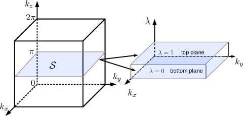
Figure 1: A planar gauge discontinuity $\mathcal{S}$ in the 3D BZ can be expanded into a fictitious slab whose thickness dimension is described by a parameter $\lambda\in[0,1]$ that interpolates smoothly between the gauge just below ($\lambda\!=\!0$) and just above ($\lambda\!=\!1$) the plane $\mathcal{S}$.

III.1 Formalism

Our strategy is to introduce a parameter $\lambda$ and define $|\psi_{m{\bf k}}(\lambda)\rangle$ in such a way that it smoothly interpolates from one gauge to the other as shown in Fig. 1, i.e.,

$$|\psi_{m{\bf k}}(\lambda)\rangle=\sum_{n}|\psi^{(0)}_{n{\bf k}}\rangle\,W_{nm}({\bf k},\lambda)$$ (13)

where

$$W({\bf k},\lambda)=e^{-i\lambda B({\bf k})}$$ (14)

where $W({\bf k},\lambda)$ is a unitary matrix defined so that $W({\bf k},0)=1$ and $W({\bf k},1)=U({\bf k})$. Note that $W({\bf k},\lambda)$ commutes with $B({\bf k})$. We shall again begin dropping the ${\bf k}$ labels, and will frequently use $W$ and $B$ below.

We then calculate the gauge-discontinuity contribution to $\theta$, denoted by $\theta_{\textrm{GD}}$, by integrating Eq. (8) over the region $\lambda\in[0,1]$, where Eq. (8) is applied in $(k_{x},k_{y},\lambda)$ space instead of $(k_{x},k_{y},k_{z})$ space. A straightforward set of calculations shows that the Berry connections in the $k_{x}$, $k_{y}$, and $\lambda$ directions are respectively

$$A_{x}(\lambda)=W^{\dagger}(\lambda)\,A^{(0)}_{x}\,W(\lambda)+iW^{\dagger}(\lambda)\,\partial_{x}W(\lambda)\;,$$ (15)

$$A_{y}(\lambda)=W^{\dagger}(\lambda)\,A^{(0)}_{y}\,W(\lambda)+iW^{\dagger}(\lambda)\,\partial_{y}W(\lambda)\;,$$ (16)

$$A_{\lambda}(\lambda)=B\;,$$ (17)

where $A_{x(y)}^{(0)}$ is the Berry connection evaluated at the bottom plane as defined earlier. We also write

$$\theta_{\textrm{GD}}=-\frac{1}{4\pi}\int d^{2}k\;G({\bf k})\;,$$ (18)

where

$$G=\int_{0}^{1}d\lambda\;{\rm Tr\,}\Big{[}A_{x}\Omega_{y\lambda}-A_{y}\Omega_{x\lambda}+A_{\lambda}\widetilde{\Omega}_{xy}-i[A_{x},A_{y}]A_{\lambda}\Big{]}$$ (19)

is the contribution from a particular ${\bf k}$. Then $G$ can be written as the sum of three contributions, $G=G_{1}+G_{2}+G_{3}$, where

$$G_{1}({\bf k})=\int_{0}^{1}d\lambda\;{\rm Tr\,}[B\,\widetilde{\Omega}_{xy}]\;,\;$$ (20)

$$G_{2}({\bf k})=\int_{0}^{1}d\lambda\;{\rm Tr\,}[A_{x}\Omega_{y\lambda}-A_{y}\Omega_{x\lambda}]\;,\;$$ (21)

$$G_{3}({\bf k})=\int_{0}^{1}d\lambda\;{\rm Tr\,}\Big{[}-i\,[A_{x},A_{y}]\,B\Big{]}\;.$$ (22)

The $G_{1}$ term is easily evaluated. Because $\widetilde{\Omega}_{xy}$ is gauge-covariant, it follows that $\widetilde{\Omega}_{xy}(\lambda)=W^{\dagger}(\lambda)\,\widetilde{\Omega}^{(0)}_{xy}\,W(\lambda)$. But $[B,W(\lambda)]=0$, so that the integrand is independent of $\lambda$, and it follows that

$$G_{1}({\bf k})={\rm Tr\,}[B\,\widetilde{\Omega}^{(0)}_{xy}]\;.$$ (23)

Here no $\lambda$ integration is needed.

In order to evaluate $G_{2}$ and $G_{3}$, we need to evaluate objects such as $\partial_{x}W(\lambda)$ in Eq. (15), which can be done by noting that the derivative of an exponential of a matrix can be written as

$$\partial_{x}{e^{-i\lambda M}}=-i\,\int_{0}^{\lambda}d\mu\;e^{-i\,\mu M}(\partial_{x}M)e^{-i\,(\lambda-\mu)M}\;.$$ (24)

This motivates us to define

$$\overline{B}_{a}(\lambda)=\int_{0}^{\lambda}d\mu\;e^{-i\mu B}\,B_{a}\,e^{i\mu B}\;,$$ (25)

where $B_{a}\equiv\partial_{a}B$. Then Eq. (14) gives

$$\partial_{a}W(\lambda)=\partial_{a}{e^{-i\lambda B}}=-i\overline{B}_{a}(\lambda)W(\lambda)$$ (26)

where $a=\{x,y\}$, and Eqs. (15-16) become

$$A_{a}(\lambda)\,=W^{\dagger}\,{\cal A}_{a}\,W\;,$$ (27)

where

$${\cal A}_{a}=A^{(0)}_{a}+\overline{B}_{a}\;.$$ (28)

The dependence on $\lambda$ is implicit.

Now for the $G_{2}$ term we need to compute terms like $\partial_{\lambda}A_{x}$. Using Eq. (27) and $\partial_{\lambda}\,W(\lambda)=-iBW(\lambda)$, it becomes

$$\partial_{\lambda}A_{x}\,=iW^{\dagger}\,[B,{\cal A}_{x}]\,W+B_{x}\;.$$ (29)

Recalling that $\Omega_{x\lambda}=\partial_{x}A_{\lambda}-\partial_{\lambda}A_{x}$ and $\partial_{x}A_{\lambda}=B_{x}$, we get a nice cancellation, and can write

$$\Omega_{x\lambda}=-i\,W^{\dagger}\,[B,{\cal A}_{x}]\,W\;,\;\\ \Omega_{y\lambda}=-i\,W^{\dagger}\,[B,{\cal A}_{y}]\,W\;.$$

Substituting these expressions into Eq. (21) then gives

$$G_{2}({\bf k})=\int_{0}^{1}d\lambda\;{\rm Tr\,}\Big{[}2i\,B\,[{\cal A}_{x},{\cal A}_{y}]\Big{]}\;.$$ (30)

As it happens, this is almost the same as the expression for $G_{3}$ in Eq. (22). Since $B$ commutes with $W$, we can use the representation-invariance and cyclic properties of the trace to write it as

$$G_{3}({\bf k})=\int_{0}^{1}d\lambda\;{\rm Tr\,}\Big{[}-i\,B\,[{\cal A}_{x},{\cal A}_{y}]\Big{]}\;.$$ (31)

Thus, this term cancels half of $G_{2}$.

Restoring the explicit $\lambda$ dependencies, we get

$$G={\rm Tr\,}\Big{[}B\,\Big{(}\widetilde{\Omega}^{(0)}_{xy}+i\int_{0}^{1}d\lambda\,[{\cal A}_{x}(\lambda),{\cal A}_{y}(\lambda)]\Big{)}\Big{]}\;,$$ (32)

which is a remarkably simple result in the end. Using Eq. (28), this can be written explicitly as

$$G({\bf k})={\rm Tr\,}\Big{[}B\Big{(}\Omega^{(0)}_{xy}+\overline{\overline{B}}_{[x,y]}+i[\,\overline{\overline{B}}_{x},A^{(0)}_{y}\,]-i[\,\overline{\overline{B}}_{y},A^{(0)}_{x}\,]\Big{)}\Big{]}\;,$$ (33)

where

$$\overline{\overline{B}}_{x}=\int_{0}^{1}d\lambda\;\overline{B}_{x}(\lambda)\;,$$ (34)

$$\overline{\overline{B}}_{y}=\int_{0}^{1}d\lambda\;\overline{B}_{y}(\lambda)\;,$$ (35)

$$\overline{\overline{B}}_{[x,y]}=i\int_{0}^{1}d\lambda\;[\,\overline{B}_{x}(\lambda),\overline{B}_{y}(\lambda)\,]\;.$$ (36)

Eq. (33) is one of the central results of this paper.

We would like to make some remarks on the formula for $\theta_{\textrm{GD}}$. First, the results are almost independent of the actual states at the top and bottom of the gauge discontinuity. The only way these come in is through the Berry potentials $A^{(0)}_{x}$ and $A^{(0)}_{y}$ and the Berry curvature $\Omega^{(0)}_{xy}$ defined on one of the planes. Second, it can easily be shown that the results are the same whether one uses the “bottom” surface in Fig. 1 as a reference and integrates up in $\lambda$, as done above, or chooses the “top” surface as a reference and integrates down. Third, the integration over the $\lambda$ axis can be carried out analytically in the basis that locally diagonalizes $B({\bf k})$, as detailed in Appendix B. Therefore only a 2D discrete integration over the k plane is needed, which is numerically efficient. Lastly, in the single-band case all quantities such as $W$, $B_{x}$ and $\overline{B}_{x}$ obviously commute with each other, leaving $G=G_{1}={\rm Tr\,}\Big{[}B\Omega_{xy}^{(0)}\Big{]}$.

In the following subsection, we discuss the properties of the $\theta_{\textrm{GD}}$ formula in the presence of $\mathcal{T}$ symmetry, showing that if a TR-symmetric gauge has been chosen in the bulk BZ and assuming that $B({\bf k})$ varies smoothly in the 2D k plane, both $\theta_{\textrm{BK}}$ and $\theta_{\textrm{GD}}$ must vanish.

III.2 Time-reversal symmetry

Consider the situation in which the system has $\mathcal{T}$ symmetry and is topologically normal, and a gauge respecting $\mathcal{T}$ symmetry has been chosen smoothly throughout the bulk BZ for the $2N$ occupied bands. For such a system we can construct $2N$ localized Wannier functions (WFs) which fall into $N$ $\mathcal{T}$-symmetric pairs,

$$\mathcal{T}|w_{n\mathbf{R},1}\rangle=-|w_{n\mathbf{R},2}\rangle\;,$$

$$\mathcal{T}|w_{n\mathbf{R},2}\rangle=|w_{n\mathbf{R},1}\rangle,$$ (37)

where $1\leq n\leq N$ is the index of a $\mathcal{T}$-symmetric pair and $\mathbf{R}$ denotes a real-space lattice vector. Typically $|w_{n\mathbf{R},1}\rangle$ and $|w_{n\mathbf{R},2}\rangle$ are chosen to diagonalize the $S_{z}$ operator in their two-dimensional subspace, so that “1” and “2” can be interpreted roughly as “spin indices.” The Fourier transform of the $\mathcal{T}$-symmetric WF pairs leads to a smooth gauge respecting $\mathcal{T}$ symmetry in the bulk BZ,

$$\mathcal{T}|\psi_{n{\bf k},1}\rangle\!=\!-|\psi_{n-{\bf k},2}\rangle\;$$

$$\mathcal{T}|\psi_{n{\bf k},2}\rangle\!=\!|\psi_{n-{\bf k},1}\rangle$$ (38)

and

$$\mathcal{T}|u_{n{\bf k},1}\rangle\!=\!-|u_{n-{\bf k},2}\rangle\;$$

$$\mathcal{T}|u_{n{\bf k},2}\rangle\!=\!|u_{n-{\bf k},1}\rangle$$ (39)

where the indices “$1$” and “$2$” are again the “spin indices”, even if the directions of the spin expectation values can have some variations with ${\bf k}$. Note that the states in Eq. (38) are of Bloch form, but in general are not the eigenstates of the Hamiltonian.

Henceforth we shall say that a gauge that obeys Eqs. (38-39) is a $\mathcal{T}$-symmetric gauge. However, in general a gauge obeying these equations is not necessarily periodic. For example, there may be a gauge discontinuity located at some boundary plane in the 3D BZ. When the $\mathbb{Z}_{2}$ index of the system is even, such a gauge discontinuity can typically be removed by smoothening the gauge without breaking the $\mathcal{T}$ symmetry. When the $\mathbb{Z}_{2}$ index is odd, however, the gauge discontinuity can never be eliminated without breaking the $\mathcal{T}$ symmetry in the gauge. For, if it could, one could again construct $\mathcal{T}$-respecting WFs, which is known to be impossible for $\mathbb{Z}_{2}$-odd insulators.

If the gauge in the bulk BZ satisfies Eq. (39), it follows that the Berry curvatures and Berry connections obey

$$A_{a}({\bf k})\!=\!\sigma_{y}\,\Big{(}A_{a}(-{\bf k})\Big{)}^{T}\,\sigma_{y},\;$$

$$\Omega_{ab}({\bf k})\!=\!-\sigma_{y}\,\Big{(}\Omega_{ab}(-{\bf k})\Big{)}^{T}\,\sigma_{y}\;,$$ (40)

where $a$ and $b$ run over the reciprocal-lattice directions. All the quantities in Eq. (40) are $2N\times 2N$ matrices. In particular, $\sigma_{y}$ denotes the outer product between the $2\times 2$ Pauli matrix $\tau_{y}$ and the $N\times N$ identity matrix, and the superscript “$T$” refers to matrix transpose for the $2N\times 2N$ matrices. Since the Berry curvature is odd in ${\bf k}$, while the Berry connections behave as even functions of ${\bf k}$, it is easy to show that both ${\rm Tr\,}\Big{[}\,A_{a}({\bf k})\,\Omega_{bc}({\bf k})\,\Big{]}$ and ${\rm Tr\,}\Big{[}\,iA_{a}({\bf k})\,[A_{b}({\bf k}),A_{c}({\bf k})]\,\Big{]}$ are canceled by their time-reversal partners at $-{\bf k}$. Therefore, the bulk integral $\theta_{\textrm{BK}}$ in Eq. (7) vanishes if a smooth $\mathcal{T}$-respecting gauge is constructed in the bulk BZ.

In particular, at the boundary plane where the gauge discontinuity is located, the wavefunctions at the bottom and top planes (say, $k_{z}=\pm\pi$) are connected via $\mathcal{T}|u^{(0)}_{n{\bf k},1}\rangle\!=\!-|u^{(1)}_{n-{\bf k},2}\rangle$ and $\mathcal{T}|u^{(0)}_{n{\bf k},2}\rangle\!=\!|u^{(1)}_{n-{\bf k},1}\rangle$, where ${\bf k}$ is now understood to be a wavevector in the 2D plane. With such a $\mathcal{T}$-respecting gauge choice, the $B$ matrix, the Berry connections, and the Berry curvature satisfy the following relationships:

$$B({\bf k})=\sigma_{y}B(-{\bf k})^{T}\sigma_{y}\;,\;$$ (41)

$$A^{(0)}_{x}({\bf k})=\sigma_{y}\,\Big{(}A^{(1)}_{x}(-{\bf k})\Big{)}^{T}\,\sigma_{y}\;,\;$$ (42)

$$A^{(0)}_{y}({\bf k})=\sigma_{y}\,\Big{(}A^{(1)}_{y}(-{\bf k})\Big{)}^{T}\,\sigma_{y}\;,\;$$ (43)

$$\Omega^{(0)}_{xy}({\bf k})=-\sigma_{y}\,\Big{(}\Omega^{(1)}_{xy}(-{\bf k})\Big{)}^{T}\,\sigma_{y}\;.$$ (44)

Again, superscripts $``(0)"$ and $``(1)"$ refer to the quantities evaluated at $\lambda\!=\!0$ and $\lambda\!=\!1$ respectively. We now show that if Eqs. (41)-(44) are satisfied, and if all the quantities involved in the Eqs. (32)-(33) vary smoothly in the 2D plane, then $\theta_{\textrm{GD}}$ must vanish.

First of all, it is straightforward to show that the first term in Eq. (32) vanishes due to $\mathcal{T}$ symmetry. As the gauge-covariant Berry curvature on the top plane ($\lambda=1$) is connected the one on the bottom plane ($\lambda=0$) via $\widetilde{\Omega}^{(1)}_{xy}\!=\!U^{\dagger}\,\widetilde{\Omega}^{(0)}_{xy}\,U$, and $U\!=\!e^{-iB}$ commutes with $B$, it follows that ${\rm Tr\,}\Big{[}B({\bf k})\widetilde{\Omega}^{(1)}_{xy}({\bf k})\Big{]}\!=\!{\rm Tr\,}\Big{[}B({\bf k})\widetilde{\Omega}^{(0)}_{xy}({\bf k})\Big{]}$. On the other hand, from Eq. (41) and Eq. (44) we know that ${\rm Tr\,}\Big{[}B({\bf k})\widetilde{\Omega}^{(0)}_{xy}({\bf k})\Big{]}\!=\!-{\rm Tr\,}\Big{[}B(-{\bf k})\widetilde{\Omega}^{(1)}_{xy}(-{\bf k})\Big{]}$, which leads to an exact cancellation for the first term.

The second term in Eq. (32) is trickier. First, from the representation-invariance of the trace and the fact that $W=e^{-i\lambda B}$ commutes with $B$, we know that ${\rm Tr\,}\Big{[}i\,B\,[{\cal A}_{x},{\cal A}_{y}]\Big{]}\!={\rm Tr\,}\Big{[}i\,B\,[A_{x}^{(\lambda)},A_{y}^{(\lambda)}]\Big{]}$. Then we claim that the Berry connection matrix at $({\bf k},\lambda)$ is connected to the one at $(-{\bf k},1-\lambda)$ via a $\mathcal{T}$ transformation

$$A_{a}^{(\lambda)}({\bf k})\!=\!\sigma_{y}\,\Big{(}A_{a}^{(1-\lambda)}(-{\bf k})\Big{)}^{T}\,\sigma_{y}\;,$$ (45)

where $A_{a}^{(\lambda)}\equiv A_{a}(\lambda)$ with $a=\{x,y\}$ as defined in Eq. (15)-(16). Eq. (45) will be proved properly in Appendix C, but if one considers $\lambda$ as the third wavevector component, Eq. (45) is indeed very intuitive. Combing Eq. (45) and Eq. (27), it follows that

$$\eta({\bf k},\lambda)=-\eta(-{\bf k},1-\lambda)\;,$$ (46)

where

$$\eta({\bf k},\lambda) = {\rm Tr\,}\Big{[}\,i\,B({\bf k})\,[{\cal A}_{x}^{(\lambda)}({\bf k}),{\cal A}_{y}^{(\lambda)}({\bf k})]\,\Big{]}\;$$ (47)

$$= {\rm Tr\,}\Big{[}\,i\,B({\bf k})\,[A_{x}^{(\lambda)}({\bf k}),A_{y}^{(\lambda)}({\bf k})]\,\Big{]}$$

is exactly the second term in Eq. (32). Therefore, that term also vanishes due to the cancellation between the integrands at $({\bf k},\lambda)$ and $(-{\bf k},1-\lambda)$. It thus follows that $\theta_{\textrm{GD}}$ has to vanish for a $\mathcal{T}$-respecting gauge choice.

IV Vortex-loop contribution

In the previous section, we derived a formula for the gauge discontinuity contribution $\theta_{\textrm{GD}}$, as expressed in Eq. (18) and Eqs. (32)-(33). We also demonstrated that for a system with $\mathcal{T}$ symmetry, if a $\mathcal{T}$-respecting gauge is constructed in the bulk BZ, and if the branch choice is made in such a way that $B({\bf k})$ varies smoothly over the entire 2D k plane, then both $\theta_{\textrm{BK}}$ and $\theta_{\textrm{GD}}$ must vanish.

However, it is well known that $\theta=\pi$ for $\mathbb{Z}_{2}$ TIs, so one may wonder where the quantized $\theta$ can come from? The answer is that, in the $\mathbb{Z}_{2}$-odd case, it is topologically impossible to insist on a branch choice such that $B$ remains smooth throughout the $(k_{x},k_{y})$ plane. In other words, the 2D k plane has to be subdivided such that one or more of the eigenvalues of $B$ change by an integer multiple of $2\pi$ when crossing from one subregion to another. We denote the boundaries of such 2D subregions as “vortex loops.” It turns out that the vortex-loop contribution is exactly $\pi$ for a $\mathbb{Z}_{2}$ TI.

In this section, we introduce such vortex loops and discuss their contribution to the $\theta$ coupling. We first propose a formal definition of a vortex loop in Sec. IV.1, and then derive a formula for the vortex-loop contribution $\theta_{\textrm{VL}}$ in Sec. IV.2. This formula turns out to be rather simple, involving two Berry phases that are accumulated as one traverses the vortex loop, one associated with the electronic Bloch-like functions and the other with the eigenvectors of $B({\bf k})$. In Sec. IV.3 we discuss several properties of our formula for $\theta_{\textrm{VL}}$. In particular, we show that in systems with $\mathcal{T}$ symmetry, and for which the gauge also respects $\mathcal{T}$ symmetry, $\theta_{\textrm{VL}}$ must be either 0 or $\pi$, corresponding to the $\mathbb{Z}_{2}$ classification of 3D $\mathcal{T}$-invariant insulators.

IV.1 What is a vortex loop

In Sec. II.2 we suggested that the complete formula for $\theta$ should include three kinds of contributions, as expressed by Eq. (11). Here we review the philosophy of the calculation, explaining why the third vortex-loop contribution $\theta_{\textrm{VL}}$ may be needed.

First, we choose a smooth gauge in the 3D bulk BZ, but the periodicity condition in the $k_{z}$ direction is relaxed. Hence some gauge discontinuity is introduced at a 2D boundary plane normal to $k_{z}$. The 3D bulk integral of Eq. (3) (excluding the boundary plane) is the $\theta_{\textrm{BK}}$ term in Eq. (11).

Next, we identify the 2D boundary as $\mathcal{S}$ . Let us define $\mathcal{S}$ as a directed area with surface normal $\hat{\mathbf{n}}$. In order to compute the integral over the 2D plane $\mathcal{S}$, $\hat{\mathbf{n}}$ is chosen in such a way that $\hat{\mathbf{x}}$-$\hat{\mathbf{y}}$-$\hat{\mathbf{n}}$ form a right-handed coordinate triad. The gauge discontinuity in the $\hat{\mathbf{n}}$ direction is given by a unitary matrix $U({\bf k})=e^{-iB({\bf k})}$ which varies smoothly with ${\bf k}$ lying in the 2D plane. Since the Hermitian matrix $B({\bf k})=i\ln U({\bf k})$ is involved in the formula for $\theta_{\textrm{GD}}$ (Eq. (33)), a branch choice for $B$ has to be made. If possible we make a branch choice so that $B({\bf k})$ is smooth and continuous over the entire k plane, but this may not always be possible or desirable. In that case $\mathcal{S}$ is divided into subregions within each of which $B({\bf k})$ is smooth and continuous. For example, Fig. 2 shows $\mathcal{S}$ divided into two subregions $\mathcal{S}_{{}_{\textrm{GD}}}$ and $\overline{\mathcal{S}}_{{}_{\textrm{GD}}}$ separated by a boundary loop $\mathcal{C}$, which we refer to as a “vortex loop.” The 2D contribution $\theta_{\textrm{GD}}$ is then computed by integrating over all subregions of $\mathcal{S}$ using Eq. (32)-(33) of Sec. III.

Since the $B$ and $U$ matrices have the same eigenvectors, the eigenvalues of $B$ may exhibit abrupt $2\pi$ jumps as they vary from one subregion to another (from $\mathcal{S}_{\rm{GD}}$ to $\mathcal{\overline{S}_{\rm{GD}}}$ in Fig. 2), even though $U$ remains smooth throughout the $(k_{x},k_{y})$ plane. The behavior of $B$ is thus singular when crossing the vortex loops. The vortex-loop contributions cannot be computed from the formula for $\theta_{\textrm{GD}}$; a new formula is needed to account for them.

In more general cases, a 3D BZ may be divided into multiple subvolumes, and these subvolumes can meet on multiple 2D surface patches with gauge discontinuities. These surface patches may further meet at one or more 1D lines or curves, which may behave as vortex loops. For such cases the definition of a vortex loop would need to be generalized, since the $U({\bf k})$ matrices obtained by approaching the meeting line from different patches are in general no longer consistent, and may not even commute with one another. We leave this more complicated situation to a future study.

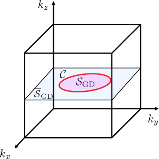
Figure 2: Schematic illustration of a 3D BZ containing a 2D plane of gauge discontinuity that is divided into two patches $\mathcal{S}_{\textrm{GD}}$ and $\overline{\mathcal{S}}_{\textrm{GD}}$ by a vortex loop (red line).

The presence or absence of vortex loops clearly depends on how the branch choice of $B$ is made in the 2D k plane. We normally try to make this choice so as to avoid vortices. If the system does not have $\mathcal{T}$ symmetry (and assuming vanishing Chern numbers), then it is usually straightforward to do this, since the eigenvalues of $B$ typically remain non-degenerate throughout the 2D k plane (degeneracies in a general Hermitian matrix are of codimension three, and so do not occur without special tuning in a 2D k plane).

However, when the system is topologically nontrivial, this may become impossible; a topological obstruction may force the existence of at least one vortex loop. In particular, if $\mathcal{T}$ symmetry is present, there must be a degeneracy between two different eigenvalues of $B$ at the four time-reversal invariant momenta (TRIM) in the 2D k plane. As a result, the topological properties of the bulk Hamiltonian become closely related to the number of vortex loops. In the same vein as the $\mathbb{Z}_{2}$ classification based on the number of surface Dirac cones,fu-prl07 when there is an odd number of vortex loops, the system is $\mathbb{Z}_{2}$-odd, corresponding to a $\mathcal{T}$-respecting topological insulator. Otherwise when the number of vortex loops is even, the system is topologically trivial. In the topologically nontrivial case, it is impossible to insist on the smoothness of all of the eigenvalues of $B$ throughout the 2D ${\bf k}$ plane. In principle the last vortex loop can be made infinitesimally small by shrinking it around one of the TRIM, but the symmetry-protected degeneracy at the TRIM prevents it from being removed completely. Therefore, we must consider the contribution from vortex loops in such topologically nontrivial phases.

On the other hand, vortex loops may be present even in topologically trivial cases unless one makes a proper branch choice to remove them. In realistic calculations, for example, one usually adopts some default branch choice for the eigenvalues of $B$ (e.g., from -$\pi$ to $\pi$), which is not necessarily the one that makes $B$ globally smooth. In such cases one has to consider both $\theta_{\textrm{GD}}$ and $\theta_{\textrm{VL}}$. In this regard, it would be useful to have a formula for the vortex loop contribution, so that one can evaluate the gauge-discontinuity contribution to $\theta$ for an arbitrary branch choice.

In the remainder of this section we will derive a formula for $\theta_{\textrm{VL}}$ and discuss properties of the formula. We will also show that in the presence of $\mathcal{T}$ symmetry in both the Hamiltonian and the gauge, the vortex-loop contribution alone determines whether the system is $\mathbb{Z}_{2}$-odd ($\theta_{\textrm{VL}}=\pm\pi$) or $\mathbb{Z}_{2}$-even ($\theta_{\textrm{VL}}=0$).

IV.2 The formula for $\theta_{\textrm{VL}}$

Let us first consider the topologically trivial case in which we can always find a proper branch choice such that $B$ remains smooth throughout the 2D plane. Assuming this has been done, now shift the $n$th eigenvalue of $B$ by $2\pi\nu(n)$ within subregion ${\mathcal{S}}_{{}_{\textrm{GD}}}$, thus creating a vortex loop $\mathcal{C}$ whose interior is ${\mathcal{S}}_{{}_{\textrm{GD}}}$ as shown in Fig. 2. The above operation is equivalent to making a different branch choice. However, a physical quantity should be independent of the branch choice, so $\theta$ should remain invariant after such an operation. Letting $\theta_{\textrm{shift}}$ be the change in $\theta_{\textrm{GD}}$ arising from this redefinition of $B$ in the interior region ${\mathcal{S}}_{{}_{\textrm{GD}}}$, it follows that we must have

$$\theta_{\textrm{VL}}=-\theta_{\textrm{shift}}\;.$$ (48)

We begin by considering a simple case in which only one of the eigenvalues of $B$ is shifted by $2\pi$ within ${\mathcal{S}}_{{}_{\textrm{GD}}}$. We make the decomposition $B=B_{0}+\Delta B$, where $B_{0}$ is the original smooth part and $\Delta B$ is the change arising from the $2\pi$ shift. We then choose to connect the states at the bottom and top planes in two steps. In the first step,

$$|\psi^{(\lambda)}_{m}\rangle=\sum_{n=1}^{N}|\psi^{(0)}_{n}\rangle\,(e^{-i\lambda\Delta B})_{nm},\;\;\;\lambda\in[0,1).$$ (49)

In the second step,

$$|\psi^{(\lambda)}_{m}\rangle=\sum_{n=1}^{N}|\psi^{(1)}_{n}\rangle\,(e^{-i(\lambda-1)B_{0}})_{nm},\;\;\;\lambda\in[1,2].$$ (50)

Note that the states at the top plane are now denoted as $|\psi^{(2)}_{m}\rangle$ instead of $|\psi^{(1)}_{m}\rangle$. In the second step, $B_{0}$ is smooth over the entire 2D BZ; one can define $\lambda^{\prime}=\lambda-1$ with $\lambda^{\prime}\in[0,1]$, and the formula for $\theta_{\textrm{GD}}$ derived in Sec. III applies. Thus, $\theta_{\textrm{shift}}=-\theta_{\textrm{VL}}$ is just the contribution to $\theta_{\textrm{GD}}$ coming from the gauge twist of Eq. (49) in the loop interior ${\mathcal{S}}_{{}_{\textrm{GD}}}$.

We assume without loss of generality that the first eigenvalue of $B$ (denoted by $b_{1}$) jumps by $2\pi$ in the subregion ${\mathcal{S}}_{{}_{\textrm{GD}}}$. Then $\Delta B$ can be written as

$$\Delta B=\begin{cases}V\,\Delta_{1}\,V^{\dagger}&\text{if }{\bf k}\in{\mathcal{S}}_{{}_{\textrm{GD}}}\\ 0&\text{otherwise}\end{cases}$$ (51)

where $\Delta_{1}$ is an $N\times N$ matrix ($N$ is the number of occupied bands), with $(\Delta_{1})_{11}=2\pi$ and all the remaining matrix elements vanishing. Here $V=(v_{1},v_{2},...,v_{N})$ is the unitary matrix whose $n$’th column $v_{n}$ is the $n$’th eigenvector of $B_{0}$. Plugging this expression for $\Delta B$ into the expression for $G$ in Eq. (33), one obtains a formula for $\theta_{\textrm{shift}}$, and $\theta_{\textrm{VL}}$ is simply the opposite of $\theta_{\textrm{shift}}$. After some considerable algebra, which we defer to Appendix D, it turns out that many terms cancel, and one obtains the surprisingly simple formula

$$\theta_{\textrm{VL}}=-\theta_{\textrm{shift}}=\Big{[}\,\phi_{1}(\mathcal{C})+\xi_{1}({\mathcal{C}})\,\Big{]}/2\;.$$ (52)

Here $\phi_{1}$ and $\xi_{1}$ are two different, but related, Berry phases that need to be computed around loop $\mathcal{C}$ (taking the positive sense of circulation with respect to the unit normal to ${\mathcal{S}}_{{}_{\textrm{GD}}}$). The second term $\xi_{1}({\mathcal{C}})$ is easier to describe; it is just the Berry phase of the $N$-component vector $v_{1}$ (the first column of $V$) as it is taken around the loop $\mathcal{C}$. To understand the first term, note that the elements of $V$ can be used to build the linear combinations

$$|\bar{\psi}^{(0)}_{n{\bf k}}\rangle=\sum_{m=1}^{N}|\psi^{(0)}_{m{\bf k}}\rangle\,V_{mn}$$ (53)

out of the Bloch functions $|\psi^{(0)}_{m{\bf k}}\rangle$ at the bottom plane ($\lambda\!=\!0$), such that

$$|\bar{\psi}^{(0)}_{1{\bf k}}\rangle=\sum_{m=1}^{N}v_{1,m}\,|\psi^{(0)}_{m{\bf k}}\rangle$$ (54)

is precisely the state whose phase is shifted by $2\pi$, while the other $N-1$ states are unaffected by $\Delta B$. Then the first term $\phi_{1}(\mathcal{C})$ in Eq. (52) is just the Berry phase of $|\bar{\psi}^{(0)}_{1{\bf k}}\rangle$ as it is carried around the loop $\mathcal{C}$. The gauge-invariance and other properties of this formula will be discussed further in the next subsection.

In the most general case, there may be multiple vortex loops $\{\mathcal{C}_{i},i=1,...L\}$ in the 2D k plane, and inside the $i$th vortex loop the $n$th eigenvalue of $B$ may be shifted by $2\pi\nu_{n}(i)$ with $\nu_{n}(i)$ being an integer. Then Eq. (52) can be generalized in a straightforward manner to

$$\theta_{\textrm{VL}}=\sum_{i}\sum_{n}\,\frac{\phi_{n}(\mathcal{C}_{i})+\xi_{n}(\mathcal{C}_{i})}{2}\;\nu_{n}(i)$$ (55)

where $\phi_{n}(\mathcal{C}_{i})$ and $\xi_{n}(\mathcal{C}_{i})$ are the Berry phases around the loop $\mathcal{C}_{i}$ of the $n$th Bloch-like state $|\bar{\psi}^{(0)}_{n{\bf k}}\rangle$ (Eq. (53)) and the $n$th eigenvector of $B$ respectively. Eq. (52), together with its generalized form Eq. (55), is the other central result of this paper.

IV.3 Discussion

We discuss the properties of Eq. (55) in this subsection. We first show that Eq. (55) is indeed gauge invariant modulo $2\pi$, which is consistent with the $2\pi$ ambiguity of $\theta$. Secondly we prove that Eq. (55) remains unchanged by interchanging the two steps corresponding to Eqs. (49) and (50). Lastly we discuss the case of $\mathcal{T}$ symmetry and conclude that as long as a gauge respecting $\mathcal{T}$ symmetry is used, $\theta_{\textrm{VL}}=\pm\pi$ or 0 depending on whether the system is $\mathbb{Z}_{2}$-odd or $\mathbb{Z}_{2}$-even, respectively.

IV.3.1 Gauge invariance

Eq. (55) is rather unexpected, as it involves the average of two Berry phases in a manner that, to our knowledge, has not been encountered before. Nevertheless, it is easy to confirm that it obeys one important property, namely, that it is well-defined modulo $2\pi$, as required for any plausible formula for $\theta$. To prove this, we first note that the only gauge freedom in Eq. (55) is a $U(1)$ gauge transformation acting on $v_{n}$, i.e., $v_{n}\to v_{n}e^{i\beta}$ (${\bf k}$-dependence is implicit). On the other hand, since $|\bar{u}^{(0)}_{n}\rangle=\sum_{m=1}^{N}|u^{(0)}_{m}\rangle\,v_{n,m}$, the same gauge transformation must also be applied to $|\bar{u}^{(0)}_{n}\rangle$, i.e., $|\bar{u}^{(0)}_{n}\rangle\to|\bar{u}^{(0)}_{n}\rangle e^{i\beta}$. As a result, if the gauge transformation has a non-zero winding number $J$, such that $\xi_{n}$ is changed by $2\pi J$, then $\phi_{n}$ must change by $2\pi J$ as well. It follows that Eq. (55) is gauge invariant modulo $2\pi$.

IV.3.2 Order of the two steps

In Sec.IV.2 we decomposed $B$ into two parts, $B=B_{0}+\Delta B$, where $B_{0}$ is the smooth part and $\Delta B$ is the contribution from the $2\pi$ shift (equal and opposite to the vortex-loop contribution). Then, in Eqs. (49) and (50), $B$ was treated in two steps in the fictitious $\lambda$ space. The first step ($0\!<\!\lambda\!<\!1$) dealt with $\Delta B$, while the second step ($1\!<\!\lambda\!<\!2$) treated the smooth part $B_{0}$. Here we would like to show that Eqs. (52) and (55) remain correct regardless of the order of the $\lambda$ integrations.

If the order is reversed, it is straightforward to show that Eq. (52) remains unchanged, but the first term $\phi_{1}$ is interpreted as the Berry phase of $|\bar{u}^{(1)}_{1}\rangle$, where $|\bar{u}^{(1)}_{1}\rangle\!=\!\sum_{n}|u^{(1)}_{n}\rangle\,v_{1,n}\!=\!\sum_{n,m}|u^{(0)}_{m}\rangle\,(e^{-iB_{0}})_{mn}\,v_{1,n}$. The Berry phases of $|\bar{u}^{(1)}_{1}\rangle$ and $|\bar{u}^{(0)}_{1}\rangle$ around the vortex loop $\mathcal{C}$ are exactly the same, because $|\bar{u}^{(1)}_{1}\rangle\!=\!\sum_{m,n,l}|\bar{u}^{(0)}_{l}\rangle\,v_{l,m}^{*}\,(e^{-iB_{0}})_{mn}\,v_{1,n}\!=\!|\bar{u}^{(0)}_{1}\rangle\,e^{-ib_{1}}$, where $b_{1}$ is the first eigenvalue of $B_{0}$. Since $b_{1}$ is smooth and single-valued everywhere in the 2D ${\bf k}$-plane, the Berry phase would not change under such a single-band transformation. Therefore, Eq. (52) and Eq. (55) remain valid even if the order of Eq. (49) and Eq. (50) is reversed.

IV.3.3 Time-reversal symmetry

We proceed to prove that $\theta_{\textrm{VL}}$ must be either $\pm\pi$ or $0$ for $\mathcal{T}$-invariant systems when the gauge in the bulk BZ is chosen to respect $\mathcal{T}$ symmetry. Again, let us consider the simple case that there is only one vortex loop $\mathcal{C}$ in the 2D k plane, and that only the first eigenvalue of $B$ is shifted by $2\pi$ inside the vortex loop. Suppose that a smooth gauge respecting $\mathcal{T}$ symmetry has been constructed in the bulk BZ, so that both the bulk integral $\theta_{\textrm{BK}}$ and the surface integral $\theta_{\textrm{GD}}$ vanish as discussed in Sec. III.2. Due to the $\mathcal{T}$-respecting gauge of Eq. (39), the $B$ matrix must satisfy Eq. (41), with two eigenvalues being degenerate at each of the four TRIM, i.e., $(0,0)$, $(0,\pi)$, $(\pi,0)$ and $(\pi,\pi)$. As a result, the vortex loop $\mathcal{C}$ has to be a “$\mathcal{T}$-symmetric” loop centered at one of the TRIM, which means that for any ${\bf k}$ on the loop $\mathcal{C}$, $-{\bf k}$ must also lie on the loop. Then it is well known that the Berry phase around such a $\mathcal{T}$-symmetric loop enclosing a degeneracy point is $\pm\pi$, as has been demonstrated in the surface states of TIs and in $\mathcal{T}$-invariant systems with giant Rashba spin-orbit splitting.shen-prb04 ; tokura-science13 It follows that $\xi_{1}\!=\!\pm\pi$ in Eq. (52)

It can be further shown that $\phi_{1}$ in Eq. (52) is exactly the same as $\xi_{1}$ as a result of the $\mathcal{T}$ symmetry. Let us first make a branch choice such that the vortex loop is negligibly small, then the Berry connection of $|\bar{u}_{1}^{(0)}\rangle$ can be expressed as

$$\bar{A}_{a,11}^{(0)} = i\,\langle{\bar{u}_{1}^{(0)}}|{\partial_{a}}{\bar{u}_{1}^{(0)}}\rangle\;$$ (56)

$$= i\sum_{m,n=1}^{N}\!V_{m1}^{*}\langle{u_{m}^{(0)}}|{\partial_{a}u_{n}^{(0)}}\rangle\,V_{n1}+i\sum_{n=1}^{N}\,V_{n1}^{*}\partial_{x}V_{n1}\;$$

$$= (V^{{}^{\dagger}}\!A_{a}^{(0)}\,V)_{11}+C_{a,11}$$

where $N$ is the number of occupied bands, $A_{a}^{(0)}$ is the Berry-connection matrix in the bottom-plane gauge with $a\!=\!\{x,y\}$, and

$$C_{a,mn}=i\sum_{l=1}^{N}V_{lm}^{*}\partial_{a}V_{ln}\;,$$ (57)

may be interpreted as the “Berry connection” in the gauge space. As the vortex loop is chosen to be vanishingly small, the variation of $|u^{(0)}_{1}\rangle$ within the vortex loop is negligible. Therefore $A_{a}^{(0)}\!=\!0$, which means $\bar{A}_{a,11}^{(0)}$ comes only from the gauge twist, i.e., $\bar{A}_{a,11}^{(0)}\!=\!C_{a,11}$. It follows that $\xi_{1}\!=\!\phi_{1}\!=\!\pm\pi$ for such a special branch choice, and $\theta_{\textrm{VL}}\!=\!\pm\pi$ according to Eq. (52).

Now suppose the loop is enlarged while preserving $\mathcal{T}$ symmetry in the shape of the loop. We showed at the end of Sec. IV.3.3 that contributions to $\theta_{\textrm{GD}}$ coming from ${\bf k}$ and $-{\bf k}$ always cancel when there is a $\mathcal{T}$-respecting gauge in the bulk, so $\theta_{\textrm{GD}}$ continues to vanish as the loop is enlarged. By the argument given around Eq. (48), this means $\theta_{\textrm{shift}}$, and therefore $\theta_{\textrm{VL}}$, cannot change as the loop is enlarged, even if the variation of $|u_{1}^{(0)}\rangle$ is no longer negligible. In other words, given a $\mathcal{T}$-respecting gauge in the bulk BZ, $\theta_{\textrm{VL}}$ must be quantized as $\pm\pi$ in the $\mathbb{Z}_{2}$-odd case regardless of the size of the vortex loop.

We can generalize the discussion to a more general case with multiple vortex loops. Obviously when there is an odd number of vortex loops, $\theta$ is still quantized as $\pm\pi$ (modulo $2\pi$). If there is an even number of vortex loops, they can either enclose an even number of TRIM or fall into $\mathcal{T}$ partners without enclosing any TRIM, and $\theta$ has to vanish (modulo $2\pi$) in either case.

V Applications

In this section, we apply our method to the Fu-Kane-Mele (FKM) model,fu-prl07 which is a 4-band tight-binding model of $s$ electrons on the diamond lattice. The model Hamiltonian is

$$H=\sum_{\langle i,j\rangle}t_{ij}c_{i}^{\dagger}c_{j}+i8\lambda_{\textrm{SO}}\sum_{\langle\langle i,j\rangle\rangle}c_{i}^{\dagger}\,\mathbf{s}\cdot(\mathbf{d}_{ij}^{1}\times\mathbf{d}_{ij}^{2})\,c_{j}\;,$$ (58)

where $t_{ij}$ is the first-neighbor spin-independent hopping and $\lambda_{\textrm{SO}}$ is the strength of the second-neighbor spin-dependent hopping generated by spin-orbit coupling (SOC); $\mathbf{d}_{ij}^{1}$ and $\mathbf{d}_{ij}^{2}$ are the two first-neighbor bond vectors connecting the two second-neighbor sites $i$ and $j$; and $\mathbf{s}\!=\!(s_{x},s_{y},s_{z})$ are Pauli matrices representing the electronic spin. Hereafter we only consider the case of half filling, i.e., two occupied bands. Setting $t_{ij}\!=\!t_{0}\!=\!1$ and $\lambda_{\textrm{SO}}\!=\!0.125$, it is easy to check that the system is a semimetal with gap closures at the three equivalent $X$ points in the BZ when the diamond-lattice symmetry is preserved. An energy gap can be opened up if an appropriate symmetry-lowering perturbation is added. For example, when the first-neighbor bond along the [111] direction is distorted, the system can be either a trivial insulator or a topological insulator depending on the strength of the bond distortion.

In order to validate our method, we need to consider the general case without $\mathcal{T}$ symmetry. Following Ref. essin-prl09, , we modify the system by applying a staggered Zeeman field with amplitude $h$, direction $\hat{\mathbf{h}}$ along [111], and opposite signs on the $A$ and $B$ sublattices. Moreover, the [111] first-neighbor bond is distorted by changing the corresponding hopping amplitude from $t_{0}$ to $3t_{0}+\delta$. We work in polar coordinates in the $(\delta,h)$ parameter space, i.e., $\delta\!=\!m\cos\beta$ and $h\!=\!m\sin\beta$. The Hamiltonian then becomes

$$H(\beta) = \!\!\sum_{\langle i,j\rangle={[111]}}\!\!\!(3t_{0}+m\cos\beta)\,c_{i}^{\dagger}c_{j}+\!\!\!\!\sum_{\langle i,j\rangle\neq{[111]}}\!\!\!t_{0}\,c_{i}^{\dagger}c_{j}$$ (59)

$$+ i8\lambda_{\textrm{SO}}\sum_{\langle\langle i,j\rangle\rangle}c_{i}^{\dagger}\,\mathbf{s}\cdot(\mathbf{d}_{ij}^{1}\times\mathbf{d}_{ij}^{2})\,c_{j}$$

$$+ m\sin\beta\sum_{i}c_{i}^{\dagger}\,\hat{\mathbf{h}}\cdot\mathbf{s}\;\tau_{z}\,c_{i}$$

where $\tau_{z}$ is the Pauli matrix defined in the space of the two sublattices. When $\beta\!=\!0$ and $\pi$, the Zeeman field vanishes so that $\mathcal{T}$ symmetry is restored, but the topological index reverses between these two cases. As $\beta$ increases from $0$ to $\pi$, the system varies smoothly from a trivial to a topological insulator along a $\mathcal{T}$-breaking path without closing the bulk energy gap.

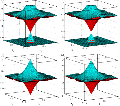
Figure 3: 3D plots of the two eigenvalues (colored red and cyan) of $B(k_{x},k_{y})\!=\!i\,\ln U(k_{x},k_{y})$ for the Fu-Kane-Mele model at half filling: (a) when the system is a TI, i.e., $\beta\!=\!\pi$, with the branch choice taken as $(-7\pi/4,\pi/4]$; (b) when $\beta\!=\!0.95\pi$, with the branch choice $(-7\pi/4,\pi/4]$; (c) when $\beta\!=\!\pi$, with the branch choice $(-5\pi/4,3\pi/4]$; and (d) when $\beta\!=\!0.95\pi$, with the branch choice $(-5\pi/4,3\pi/4]$. The wavevectors $k_{x}$ and $k_{y}$ are reduced such that $k_{j}\in[0,1]$ generates the 2D BZ.

Setting $t_{0}\!=\!1$, $\lambda_{\textrm{SO}}\!=\!0.125$, and $m\!=\!0.5$, we first study the behavior of the $B$ matrix of Eq. (12) in the $(k_{x},k_{y})$ plane with the branch choice $(-7\pi/4,\pi/4]$ for the eigenvalues of $B({\bf k})$. As shown in Fig. 3(a), when the system is in the $\mathbb{Z}_{2}$-odd phase ($\beta\!=\!\pi$) there is a single vortex loop surrounding the TRIM at $(\pi,\pi)$. Within the loop, one of the eigenvalues of $B$ (shown in cyan) is shifted by $2\pi$, while the other eigenvalue remains continuous. Moreover, as a result of $\mathcal{T}$ symmetry, the two eigenvalues of $B$ are degenerate at each TRIM, leading to quantized Berry phases as discussed in Sec. IV.3. Fig. 3(b) shows what happens if $\mathcal{T}$ symmetry is broken by setting $\beta\!=\!0.95\pi$. Even though the vortex loop is still present for this value of $\beta$, the two eigenvalues of $B$ are no longer degenerate at the TRIM.

As discussed in Sec. IV.1, for the $\mathbb{Z}_{2}$-odd case a vortex loop has to be present regardless of the branch choice. The best one can do is to compress the vortex loop to one of the TRIM in the 2D plane. This is illustrated in Fig. 3(c), where the system of Fig. 3(a) is reanalyzed using a branch choice of $(-5\pi/4,3\pi/4]$. Now the vortex loop is compressed to the point $(\pi,\pi)$ in the $(k_{x},k_{y})$ plane. On the other hand, using the same branch choice, the vortex loop can be completely removed when $\beta\!=\!0.95\pi$, as shown in Fig. 3(d).

Using the methods developed in Secs. III and IV, we have calculated the total axion response $\theta$ along the path from $\beta\!=\!0$ to $\pi$ by taking the sum of $\theta_{\textrm{BK}}$, $\theta_{\textrm{GD}}$ and $\theta_{\textrm{VL}}$. We first explain the procedures for these calculations before discussing any specific results. The parallel-transport technique,MLWF-1 which is detailed in Appendix A, is heavily used in the gauge construction. As discussed earlier, the basic idea is that we first construct a smooth gauge in the bulk BZ that is periodic only in the $k_{x}$ and $k_{y}$ directions. Then we can extract the unitary matrix $U(k_{x},k_{y})$ describing the gauge discontinuity (Eq. (9)) by calculating the overlap matrix between the Bloch states in the top-plane and bottom-plane gauges. The logarithm of $U(k_{x},k_{y})$, taken with a given branch choice, is the $B$ matrix. We also need to calculate the Berry curvature and Berry connections either in the top-plane gauge or in the bottom-plane gauge. Then all the formulas derived in previous sections can be applied.

To be specific, we first need to construct a smooth and periodic gauge on an arbitrary $(k_{x},k_{y})$ plane. For definiteness suppose this is the $k_{z}\!=\!0$ plane. We start by constructing the “1D maxloc” gauge (see Appendix A) along the $k_{y}$ direction at $k_{x}\!=\!0$, then make a set of separate parallel transports from $k_{x}\!=\!0$ to $k_{x}\!=\!2\pi$ at each $k_{y}$, leaving some gauge discontinuity at the line $k_{x}\!=\!2\pi$ denoted by $Y(k_{y})\!=\!e^{-iD(k_{y})}$. We then apply a local (in ${\bf k}$ space) unitary transformation $R(k_{x},k_{y})\!=\!e^{ik_{x}D(k_{y})/2\pi}$ to the occupied states at each point in the 2D plane to smooth out this discontinuity. In the above operation, we have maintained the smoothness of the gauge because the $R$ matrix is defined so as to be smooth in the interior of the 2D plane. Furthermore, the gauge discontinuity at the boundary line $k_{x}\!=\!2\pi$ has been removed. After these operations, we have successfully constructed a smooth and periodic gauge in the chosen $k_{z}\!=\!0$ plane.

Taking this gauge in the $k_{z}\!=\!0$ plane as a “reference gauge,” at each $(k_{x}$, $k_{y})$ we further carry out two sets of parallel transports along the positive and negative $k_{z}$ directions from $k_{z}\!=\!0$ to $k_{z}\!=\!\pm\pi$. However, now the periodicity condition in $k_{z}$ is relaxed so that the states are as aligned to each other as possible in the interval $k_{z}\!\in\!(-\pi,\pi)$. This makes the numeric convergence of the bulk integral, Eq. (7), much easier. The overall result is a gauge that is smooth everywhere in the bulk BZ and periodic only in the $k_{x}$ and $k_{y}$ directions. Some gauge discontinuity is left at the plane $k_{z}\!=\!\pm\pi$, which is described by the $U$ matrix introduced in Sec. II.2. We are now prepared to apply the formulas derived in Sec. III and Sec. IV to our system of interest.

The above procedures have to be implemented with caution if the system is in the $\mathbb{Z}_{2}$-odd phase. In this case, it is desirable to construct a bulk gauge respecting $\mathcal{T}$ symmetry, so that both $\theta_{\textrm{BK}}$ and $\theta_{\textrm{GD}}$ vanish, and the remaining contribution from $\theta_{\textrm{VL}}$ is quantized as $\pm\pi$. For a 3D strong TI, however, the 2D $\mathbb{Z}_{2}$ indices for the $k_{z}\!=\!0$ plane and the $k_{z}\!=\!\pi$ plane must be opposite. Since it is impossible to construct a smooth and periodic $\mathcal{T}$-symmetric gauge in the $\mathbb{Z}_{2}$-odd plane,fu-prb06 one has to select the $\mathbb{Z}_{2}$-even plane for the construction of the reference gauge. Since standard methods for computing $\mathbb{Z}_{2}$ indices are now available,soluyanov-prb11 ; dai-prb11 even in the absence of $\mathcal{P}$ symmetry, the selection of the $\mathbb{Z}_{2}$-even plane should be straightforward.

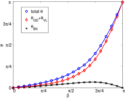
Figure 4: Axion response $\theta$ for the Fu-Kane-Mele model. Blue circles denote the total response. Red diamonds indicate the contribution from the gauge discontinuity, including both the 2D surface integral $\theta_{\textrm{GD}}$ and the 1D vortex-loop integral $\theta_{\textrm{VL}}$. Black crosses represent the contribution from the bulk integral without enforcing periodicity in the $k_{z}$ direction.

The axion response $\theta$ for the FKM model is shown as blue circles in Fig. 4. As $\beta$ increases from 0 to $\pi$, the system evolves from a $\mathbb{Z}_{2}$-even to a $\mathbb{Z}_{2}$-odd phase without closing the bulk energy gap, and $\theta$ increases smoothly from $0$ to $\pi$. When $\beta$ is below $\sim\!0.85\pi$, a conventional 3D numeric integral using a fully smooth and periodic gauge throughout the BZ is still practical, and the results obtained from our method are perfectly consistent with those from the conventional method in this regime. Nevertheless, it is much easier to reach numerical convergence using our method. For example, when $\beta\!=\!0.85\pi$, the conventional method requires a $120\times 120\times 120$ ${\bf k}$ mesh to reduce the numerical error to within $1\%$, while only an $80\times 80\times 80$ ${\bf k}$ mesh is needed to obtain the same numerical convergence using our method. When $\beta$ exceeds $0.85\pi$, it becomes impractical to get the expected convergence using the conventional method, and the advantage of our method becomes more obvious. For example, when $\beta\!=\!0.9\pi$, the bulk integral using the conventional method (enforcing periodicity in all three directions) does not converge to the expected value even for a $200\!\times\!200\!\times\!200$ ${\bf k}$ mesh, while it converges easily for a $100\!\times\!100\!\times\!80$ ${\bf k}$ mesh for $\theta_{\textrm{BK}}$ in our method. The 2D integral $\theta_{\textrm{GD}}$ also converges with a $100\!\times\!100$ 2D ${\bf k}$ mesh after the bulk gauge is constructed. The convergence for the vortex-loop integral ($\theta_{\textrm{VL}}$) is even easier; discretizing the loop into $\sim$40 ${\bf k}$ points would typically be enough to get converged values of Berry phases (a $100\!\times\!100$ 2D ${\bf k}$ mesh discretizes the vortex loop into 41 ${\bf k}$ points when $\beta\!=\!0.9\pi$ with the branch choice $(-7\pi/4,\pi/4]$). Summing over all three terms $\theta_{\textrm{BK}}$, $\theta_{\textrm{GD}}$ and $\theta_{\textrm{VL}}$ eventually leads to the results indicated by blue circles in Fig. 4.

Note that the axion coupling of the FKM model has been calculated previously using other methods. In Ref. essin-prl09, , when $\beta$ approaches $\pi$, Essin et al. switched to some indirect methods such as calculating the total polarization of a finite sample subject to a weak external magnetic field; while in Ref. maryam-prl15, Taherinejad et al. calculated $\theta$ in the “hybrid-Wannier-function” basis. The results obtained from our method also agree very well with these previous results when $\beta$ is close to $\pi$.

As shown in Fig. 4, it is helpful to decompose the total $\theta$ into the bulk-BZ integral $\theta_{\textrm{BK}}$ and the remainder $\theta_{\textrm{GD}}+\theta_{\textrm{VL}}$, which are indicated by black crosses and red diamonds respectively. One finds that as $\beta$ increases, $\theta_{\textrm{GD}}+\theta_{\textrm{VL}}$ becomes more and more dominant. Eventually when $\beta\!=\!\pi$, $\theta$ comes entirely from by the vortex-loop term, which equals $\pi$, because both $\theta_{\textrm{GD}}$ and $\theta_{\textrm{BK}}$ vanish due to the $\mathcal{T}$-symmetric bulk gauge.

It should be noted that none of the three terms $\theta_{\textrm{BK}}$, $\theta_{\textrm{GD}}$ or $\theta_{\textrm{VL}}$, is independently gauge invariant. As the size of the vortex loop is dependent on the branch choice, in general both $\theta_{\textrm{VL}}$ and $\theta_{\textrm{GD}}$ are branch-choice dependent, but the sum of them should remain invariant if the bulk gauge is fixed.

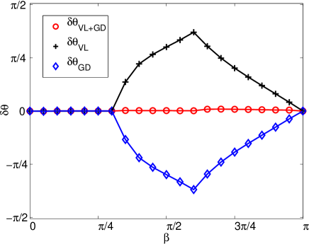
Figure 5: Difference between the $\theta$ values calculated with two different branch choices (see text) for the Fu-Kane-Mele model. The blue diamonds, black pluses and red circles denote the differences for $\theta_{\textrm{GD}}$, $\theta_{\textrm{VL}}$ and $\theta_{\textrm{VL}}+\theta_{\textrm{GD}}$ respectively.

The above statement is verified by computing $\theta_{\textrm{VL}}$ and $\theta_{\textrm{GD}}$ using different branch choices for a given gauge in the bulk BZ as shown in Fig. 5, where the blue diamonds (black plus signs) denote the difference between the values of $\theta_{\textrm{GD}}$ ($\theta_{\textrm{VL}}$) calculated using the two different branch choices $(-2\pi,0]$ and $(-7\pi/4,\pi/4]$. For the first branch choice $(-2\pi,0]$, a vortex loop appears when $\beta\!=\!0.35\pi$ and then grows as $\beta$ increases, while for the other branch choice the $B$ matrix remains continuous throughout the 2D ${\bf k}$ plane until $\beta\!=\!0.65\pi$. It is clearly seen from Fig. 5 that both $\theta_{\textrm{VL}}$ and $\theta_{\textrm{GD}}$ depend on the branch choice. On the other hand, the red circles in Fig. 5 represent the difference of the total $\theta_{\textrm{GD}}+\theta_{\textrm{VL}}$ computed for the two different branch choices. The difference remains vanishingly small throughout the adiabatic path, thus numerically confirming that the sum of $\theta_{\textrm{VL}}$ and $\theta_{\textrm{GD}}$ remains branch-choice-invariant.

Besides the branch choice, there is still the freedom to choose the gauge in the bulk BZ; both $\theta_{\textrm{BK}}$ and $\theta_{\textrm{GD}}+\theta_{\textrm{VL}}$ depend on this gauge choice. However, since the bulk gauge was chosen in such a way as to align the states with each other as much as possible in the $k_{z}$ direction, the bulk integral $\theta_{\textrm{BK}}$ is typically small, explaining why $\theta_{\textrm{GD}}+\theta_{\textrm{VL}}$ dominates over $\theta_{\textrm{BK}}$ in Fig. 4.

VI Summary

To summarize, we have developed a new method for computing the Chern-Simons axion coupling $\theta$. The basic idea is to relax the periodicity condition of the gauge in one of the ${\bf k}$ directions, thus introducing a gauge discontinuity residing at a 2D k plane in the BZ. The total $\theta$ then has both a bulk contribution $\theta_{\textrm{BK}}$, obtained as a conventional 3D integral over the interior of the bulk BZ, and a gauge-discontinuity contribution $\theta_{\textrm{GD}}$, which is expressed as a 2D integral over the gauge-discontinuity plane as given by Eqs. (18) and (33). Moreover, it may happen that discontinuities are introduced for a given branch choice of $B({\bf k})$, the logarithm of the unitary connection matrix describing the gauge discontinuity; this is sometimes done for convenience, but may also be required depending on the topological properties of the system. In such cases the gauge-discontinuity plane is further divided into subregions by 1D vortex loops, and one must also consider the vortex-loop contribution as expressed in Eq. (55). The total $\theta$ is then $\theta\!=\!\theta_{\textrm{BK}}+\theta_{\textrm{GD}}+\theta_{\textrm{VL}}$.

Since the periodicity condition in one of the k directions (e.g., the $k_{z}$ direction) is relaxed, the gauge in the bulk BZ does not twist as strongly as in the case when both periodicity and smoothness are required. This leads to improved numerical convergence of the 3D bulk integral of Eq. (7). The loss of periodicity is compensated by extra contributions from the gauge discontinuity ($\theta_{\textrm{GD}}$) and possible vortex loops ($\theta_{\textrm{VL}}$). The formulas for both terms turn out to be fairly simple and can be implemented numerically without difficulty.

It is interesting to note that if a $\mathcal{T}$-respecting gauge has been constructed in the bulk BZ for a $\mathcal{T}$-invariant system, then both $\theta_{\textrm{BK}}$ and $\theta_{\textrm{GD}}$ must vanish. The only surviving term $\theta_{\textrm{VL}}$ is then either 0 or $\pi$, corresponding to the $\mathbb{Z}_{2}$ classification of 3D $\mathcal{T}$-invariant insulators. Our theory thus provides a new interpretation to the formally quantized magnetoelectric response in TIs.

We have applied our method to the Fu-Kane-Mele model with staggered Zeeman field. We calculated the axion response for the model along a $\mathcal{T}$-breaking path connecting the $\mathbb{Z}_{2}$-even and $\mathbb{Z}_{2}$-odd phases. Our results agree well with the previous results obtained from other methods.essin-prl09 ; maryam-prl15 In particular, we find that the gauge-discontinuity contribution $\theta_{\textrm{GD}}+\theta_{\textrm{VL}}$ becomes increasingly dominant as the system approaches the $\mathbb{Z}_{2}$-odd phase. In the TI phase, as mentioned above, $\theta$ is completely determined by the vortex-loop term for a $\mathcal{T}$-symmetric gauge in the bulk BZ, and the $\pi$ quantization of $\theta$ is due to the $\pi$ quantization of the Berry phase around a single vortex loop.

Our method may be generalized to the case that the 3D BZ is divided into multiple subvolumes. These subvolumes may meet each other at multiple 2D surface patches, each with its own gauge discontinuity. The surface patches may further meet at 1D lines or curves, which may be vortex loops. In such more complicated cases, the formula for $\theta_{\textrm{GD}}$ still applies, but the definition of a vortex line has to be generalized to the situation that the $U$ matrices obtained by approaching the vortex loop from different surface patches may no longer commute with each other. Thus the formula for $\theta_{\textrm{VL}}$ may need to be modified. We leave this problem for future study.

From a theoretical point of view, the results presented in this paper provide a step forward in understanding the axion coupling in 3D insulators. We introduced the gauge-discontinuity and vortex-loop contributions to $\theta$, and found that the latter can be expressed in an unusual way as the sum of two closely related Berry phases. From the perspective of first-principles calculations, we have proposed a numerically efficient method for computing the Chern-Simons orbital ME coupling in solids. Our method can be implemented straightforwardly in standard first-principles code packages. This makes it possible to compute the orbital ME coefficients efficiently for realistic materials, thus facilitating the search for functional materials with enhanced ME couplings.

Appendix A Parallel transport

In this section, we discuss how to carry out the parallel transport operation and construct the “1D maxloc” gauge starting from a set of occupied eigenstates with an arbitrary gauge on a given k path. The basic idea is to recursively make the (periodic part of) the Bloch states at each ${\bf k}$ point on the path as aligned as possible with the states at the immediately previous ${\bf k}$ point. If the ${\bf k}$ path is chosen to be a closed loop, the states obtained at the end of the loop may differ from those at the start by some phase factors after the parallel-transport operation, with the mismatch giving exactly the Berry phases of the Bloch states around the loop. The Berry phases accumulated along the ${\bf k}$ path can be smeared out by smoothly distributing the phase to the states at every ${\bf k}$ point on the loop. After such an operation, one obtains a gauge which is both smooth and periodic along the path (loop), and which we refer to as a 1D maxloc gauge.MLWF-1

To be specific, let us consider a set of occupied bands $|u_{n{\bf k}}\rangle$, with $n=1,...N$, which are isolated from other bands (in energy) everywhere in the BZ. Let us take a closed ${\bf k}$ path along $k_{z}$ running from 0 to $2\pi$, with the path sampled by $J$ discrete points, so that ${\bf k}_{j}=2\pi(j-1)\hat{z}/J$. Assume that the eigenstates with some arbitrary gauge $|u_{n{\bf k}_{j}}^{0}\rangle$ are given for $j=1,...J$, and a periodic gauge is chosen at the $(J+1)$th point so that $|u_{n{\bf k}_{J+1}}^{0}\rangle=e^{-i2\pi z}|u_{n{\bf k}_{1}}^{0}\rangle$. To carry out the parallel transport, we need to insist that each overlap matrix between the occupied states at ${\bf k}_{j+1}$ and ${\bf k}_{j}$, i.e., $M_{mn}(j)={\langle u_{m{\bf k}_{j}}^{0}|u_{n{\bf k}_{j+1}}^{0}\rangle}$, is positive-definite Hermitian. This can be done as follows. At each ${\bf k}_{j}$, make a singular-value decomposition to the overlap matrix $M_{j}=V_{j}\Sigma_{j}W^{\dagger}_{j}$, where $V$ and $W$ are unitary and $\Sigma$ is real positive diagonal. Then apply a unitary transformation $L_{j}=W_{j}V^{\dagger}_{j}$ to $|u_{n{\bf k}_{j+1}}^{0}\rangle$, $|\widetilde{u}_{n{\bf k}_{j+1}}\rangle=\sum_{m=1}^{N}L_{j,mn}|u_{m{\bf k}_{j+1}}^{0}\rangle$, so that the overlap matrix between the unitarily transformed states at neighboring ${\bf k}$ points becomes positive-definite Hermitian. If one repeats such an operation from $j=1$ to $j=J$, the states will become as aligned to each other as possible at all ${\bf k}$ points on the path. However, there is still some gauge discontinuity left at the boundary, $|\widetilde{u}_{n{\bf k}_{J+1}}\rangle=e^{-i2\pi z}\sum_{m}\Lambda_{mn}|\widetilde{u}_{m{\bf k}_{1}}\rangle$, where $\Lambda$ is a unitary matrix. The logarithms of the eigenvalues of $\Lambda$, $\beta_{n}=-i\ln\lambda_{n}$, are then identified as the non-Abelian Berry phases (also known as Wilson loop eigenvalues) of the Bloch states.

The gauge obtained from the parallel-transport operation is smooth along the ${\bf k}$ path, but not periodic. To restore the periodicity, we need to rotate all the states on the ${\bf k}$ path to the basis that diagonalizes $\Lambda$, i.e., $|u^{\prime}_{n{\bf k}_{j}}\rangle=\sum_{m=1}^{N}|\widetilde{u}_{m{\bf k}_{j}}\rangle\,L_{mn}$, where $L$ is the eigenvector matrix of $\Lambda$. Then we gradually smear out the discontinuity by applying the following phase twist to the states at ${\bf k}_{j}$: $|u_{n{\bf k}_{j}}\rangle=e^{-i(j-1)\beta_{n}/J}|u^{\prime}_{n{\bf k}_{j}}\rangle$. This results in a “1D maxloc gauge” that is both smooth and periodic along the ${\bf k}$ path.

Appendix B Integration over $\lambda$ in the formula for $\theta_{\textrm{GD}}$

In deriving the expression in Eq. (18) for the gauge discontinuity contribution $\theta_{\textrm{GD}}$ in Sec. III.1, we arrived at Eq. (33) involving the quantities $\overline{\overline{B}}_{x}$, $\overline{\overline{B}}_{y}$, and $\overline{\overline{B}}_{[x,y]}$ which were expressed as integrals over $\lambda$ in Eqs. (34-36). We show here that these three quantities can all be computed analytically in the sense that the $\lambda$ integral does not have to be discretized.

The plan is as follows. Suppose that $A^{(0)}_{x}({\bf k})$, $A^{(0)}_{y}({\bf k})$, $\Omega^{(0)}_{xy}({\bf k})$, $B({\bf k})$, $B_{x}({\bf k})$, and $B_{y}({\bf k})$ are known. The first term in Eq. (33) is independent of $\lambda$ and is trivial. For the remaining terms, at each ${\bf k}$, locally diagonalize $B({\bf k})$, then transform all of the matrices $A^{(0)}_{x}({\bf k})$, $A^{(0)}_{y}({\bf k})$, $B_{x}({\bf k})$, and $B_{y}({\bf k})$ to the basis that locally diagonalizes $B({\bf k})$, i.e.,

$$B({\bf k})\to V^{\dagger}({\bf k})\,B({\bf k})\,V({\bf k}),\;$$

$$B_{a}({\bf k})\to V^{\dagger}({\bf k})\,B_{a}({\bf k})\,V({\bf k}),\;$$

$$A_{a}({\bf k})\to V^{\dagger}({\bf k})\,A_{a}({\bf k})\,V({\bf k}),\;$$

$$\Omega_{xy}({\bf k})\to V^{\dagger}({\bf k})\,\Omega_{xy}({\bf k})\,V({\bf k})\;,$$ (60)

where $V({\bf k})$ is the eigenvector matrix of $B({\bf k})$, and $a=\{x,y\}$. Then one can compute the trace in this basis. Letting $B_{mn}=b_{n}\,\delta_{mn}$, we find

$$\overline{B}_{x,mn}(\lambda) = \int_{0}^{\lambda}d\mu\;e^{-i\mu b_{m}}\,B_{x,mn}\,e^{i\mu b_{n}}\;$$ (61)

$$= g_{mn}(\lambda)\,B_{x,mn}\;,$$

where

$$g_{mn}(\lambda)=\frac{e^{-i\lambda(b_{m}-b_{n})}-1}{-i(b_{m}-b_{n})}\;.$$ (62)

Then

$$\overline{\overline{B}}_{x,mn} = \Big{(}\int_{0}^{1}g_{mn}(\lambda)\,d\lambda\Big{)}\;B_{x,mn}\;$$

$$= \Big{(}\frac{e^{i(b_{n}-b_{m})}-1}{-(b_{n}-b_{m})^{2}}-\frac{1}{i(b_{n}-b_{m})}\Big{)}\;B_{x,mn}\;$$

and

$$\overline{\overline{B}}_{{[x,y]}mn}= i\sum_{l}\Big{(}\int_{0}^{1}g_{ml}(\lambda)\,g_{ln}(\lambda)\,d\lambda\Big{)}\,\times\;$$ (64)

$$\Big{(}B_{x,ml}\,B_{y,ln}-B_{y,ml}\,B_{x,ln}\Big{)}\;.$$

Because we are interested in the trace of $B\,\overline{\overline{B}}_{[x,y]}$ in the basis that $B$ is locally diagonal, only the diagonal matrix elements of $\overline{\overline{B}}_{[x,y]}$ are relevant. After carrying out the integral in Eq. (64) one obtains the following expression:

$$\overline{\overline{B}}_{{[x,y]}nn}= i\sum_{m}\Big{(}\frac{2}{(b_{n}-b_{m})^{2}}-\frac{2\sin(b_{m}-b_{n})}{(b_{m}-b_{n})^{3}}\Big{)}\times\;$$ (65)

$$\Big{(}B_{x,nm}B_{y,mn}-B_{y,nm}B_{x,mn}\Big{)}\;.$$

If two eigenvalues $b_{m}$ and $b_{n}$ are degenerate, one needs to take the limit $(b_{n}-b_{m})\to 0$. It turns out that both quantities are finite:

$$\lim_{b_{n}\to b_{m}}\overline{\overline{B}}_{x,mn}=B_{x,mn}/2\;,$$ (66)

and

$$\lim_{b_{m}\to b_{n}}\overline{\overline{B}}_{{[x,y]}nn}=\frac{i}{3}\Big{(}B_{x,nm}B_{y,mn}-B_{y,nm}B_{x,mn}\Big{)}\;.$$ (67)

Of course the entire calculation still has to be done on a discretized mesh on the ${\bf k}$ plane, with finite-difference expressions used to evaluate objects like $A^{(0)}_{x}({\bf k})$, so it it not “exact”. However, it is convenient that we don’t have to discretize the $\lambda$ axis, instead doing all $\lambda$ integrals analytically.

Appendix C Derivation of Eq. (45)

In Sec. III.2 we considered the effect of time-reversal symmetry on the gauge discontinuity on the boundary plane and showed that $\theta_{\textrm{GD}}$ has to vanish for a $\mathcal{T}$-respecting choice of gauge. The demonstration rested on the use of Eq. (45), which was only introduced heuristically there.

Here we prove it properly. From Eqs. (27), (28) and (25), we know that

$$A_{a}^{(\lambda)}=\widetilde{A}_{a}^{(\lambda)}+\Gamma_{a}(0,\lambda)$$ (68)

where

$$\widetilde{A}_{a}^{(\lambda)}=W^{\dagger}(\lambda)\,A_{a}^{(0)}\,W(\lambda)\;,$$ (69)

and the function $\Gamma_{a}(\lambda_{1},\lambda_{2})$ is defined as

$$\Gamma_{a}(\lambda_{1},\lambda_{2})=\int_{\lambda_{1}}^{\lambda_{2}}d\mu\,W^{\dagger}(\mu)\,B_{a}\,W(\mu)\;.$$ (70)

Letting $\lambda=1$, we get the expression

$$A_{a}^{(1)}=\widetilde{A}_{a}^{(1)}+\Gamma_{a}(0,1),$$ (71)

Applying a unitary transformation $W(1-\lambda)$ to the matrix $A_{a}^{(1)}$, one obtains

$$W(1-\lambda)\,A_{a}^{(1)}\,W^{\dagger}(1-\lambda) = \widetilde{A}_{a}^{(\lambda)}+\Gamma_{a}(\lambda-1,\lambda)\;,$$

$$= A_{a}^{(\lambda)}+\Gamma_{a}(\lambda-1,0)\;,$$

where a variable transformation $(\lambda+\nu-1)\!\to\!\mu$ has been made to obtain the second term $\Gamma_{a}(\lambda-1,\lambda)$ on the RHS of the first line in Eq. (LABEL:eq:wA1w). The integral from $\lambda-1$ to $\lambda$ in $\Gamma_{a}(\lambda-1,\lambda)$ is further divided into two integrals: one from $\lambda-1$ to 0, and the other from 0 to $\lambda$. $A_{a}^{(\lambda)}$ in the second line is then obtained by combining the integral from $0$ to $\lambda$ together with $W^{\dagger}(\lambda)\,A_{a}^{(0)}\,W(\lambda)$ (Eq. (68)). Therefore

$$A_{a}^{(\lambda)}=W(1-\lambda)\,A_{a}^{(1)}\,W^{\dagger}(1-\lambda)\;-\Gamma_{a}(\lambda-1,0)$$ (73)

and it immediately follows that

$$A_{a}^{(1-\lambda)} = W(\lambda)\,A_{a}^{(1)}\,W^{\dagger}(\lambda)-\Gamma_{a}(-\lambda,0)\;$$

$$= W(\lambda)\,A_{a}^{(1)}\,W^{\dagger}(\lambda)-\int_{0}^{\lambda}d\mu\,W(\mu)\,B_{a}\,W^{\dagger}(\mu)\;,$$

(74)

where we let $\mu\to-\mu$ in going from the first to the second line in Eq. (74). Equation (45 then follows by combining Eq. (42)-(43) and Eq. (74):

$$A_{a}^{(1-\lambda)}(-{\bf k})\; = e^{-i\lambda B(-{\bf k})}\,A_{a}^{(1)}(-{\bf k})\,e^{i\lambda B(-{\bf k})}-\int_{0}^{\lambda}d\mu\,e^{-i\mu B(-{\bf k})}\,B_{a}(-{\bf k})\,e^{i\mu B(-{\bf k})}\;$$ (75)

$$= \sigma_{y}\,e^{-i\lambda B^{T}({\bf k})}\,\Big{(}A_{a}^{(0)}({\bf k})\Big{)}^{T}\,e^{i\lambda B^{T}({\bf k})}\,\sigma_{y}+\sigma_{y}\,\int_{0}^{\lambda}d\mu\,e^{-i\mu B^{T}({\bf k})}\,B_{a}^{T}({\bf k})\,e^{i\mu B^{T}({\bf k})}\,\sigma_{y}\;$$

$$= \sigma_{y}\,\Big{(}W^{\dagger}(\lambda)\,A_{a}^{(0)}({\bf k})\,W(\lambda)+\int_{0}^{\lambda}d\mu\,W^{\dagger}(\mu)\,B_{a}({\bf k})\,W(\mu)\Big{)}^{T}\,\sigma_{y}\;.$$

The last line in Eq. (75) is simply $\sigma_{y}\,\Big{(}A_{a}^{(\lambda)}({\bf k})\Big{)}^{T}\,\sigma_{y}$, thus proving Eq. (45) and thereby confirming that $\theta_{\textrm{GD}}$ vanishes for a TR-invariant gauge.

Appendix D Derivation of Eq. (52)

In Sec. IV.2 we proposed a formula for the vortex-loop contribution as expressed in Eq. (52). We only explained the main idea there, and the formula was introduced without proof. Here we provide a rigorous derivation.

To derive Eq. (52), it is convenient to decompose $G({\bf k})$ into four terms $G_{1}$, $G_{2}$, $G_{3}$ and $G_{4}$ corresponding to the four terms on the right-hand side (RHS) of Eq. (33):

$$G_{1}=B\,\Omega^{(0)}_{xy}\;,$$ (76)

$$G_{2}=iB\,[\,\overline{B}_{x}(\lambda),\overline{B}_{y}(\lambda)\,]\;,$$ (77)

$$G_{3}=iB\,[\,A^{(0)}_{x},\overline{B}_{y}(\lambda)\,]\;,$$ (78)

$$G_{4}=iB\,[\,\overline{B}_{x}(\lambda),A^{(0)}_{y}\,]\;.$$ (79)

Since all the quantities such as $\Omega_{xy}$ and $A_{x(y)}$ are defined in the bottom-plane gauge, we will drop the superscript “(0)” (indicating the bottom-plane gauge) in later steps. Recalling that the change $\Delta B$ in the interior region was expressed in Eq. (51) as $V\Delta_{1}{V}^{\dagger}$, where $V$ is the unitary matrix that diagonalizes $B$ and $\Delta$ is diagonal with $2\pi$-integer entries, we can transform the needed matrices to the $B$-diagonal representation via

$$A_{a}^{\prime}=V^{\dagger}\,A_{a}\,V\;,$$ (80)

$$\Omega_{xy}^{\prime}=V^{\dagger}\,\Omega_{xy}\,V\;,$$ (81)

$$\overline{B}_{a}^{\prime}=V^{\dagger}\,\overline{B}_{a}\,V\;.$$ (82)

We will prove Eq. (52) by explicitly calculating the four terms in Eqs. (76)-(79).

D.1 The $G_{1}$ term

Plugging Eq. (51) first into the expression for $G_{1}$ in Eq. (76), one obtains

$${\rm Tr\,}\Big{[}\,G_{1}\,\Big{]} = {\rm Tr\,}\Big{[}\,V\,\Delta_{1}\,V^{\dagger}\Omega_{xy}\,V\,V^{\dagger}\,\Big{]}\;$$ (83)

$$= {\rm Tr\,}\Big{[}\,\Delta_{1}\,V^{\dagger}\Omega_{xy}\,V\,\Big{]}\;.$$

Note that $\Omega_{xy}^{\prime}=V^{\dagger}\,\Omega_{xy}\,V$ is associated with the Berry curvature of the Bloch states in the bottom-plane gauge that are unitarily transformed by $V$: $|\bar{u}^{(0)}_{n}\rangle=\sum_{m=1}^{N}|u^{(0)}_{m}\rangle\,V_{mn}$. One can express the Berry curvature of $|\bar{u}^{(0)}_{n}\rangle$ (denoted by $\bar{\Omega}_{xy}$) in terms of $A_{x}$, $A_{y}$, $\Omega_{xy}$, $V$ and the partial derivatives of $V$,

$$\bar{\Omega}_{xy}=\Omega_{xy}^{\prime}+\Lambda_{xy}+i[\,C_{x},A_{y}^{\prime}\,]-i[\,C_{y},A_{x}^{\prime}\,]\;,$$ (84)

where $C_{x}$ and $C_{y}$ are defined in Eq. (57), and

$$\Lambda_{xy}=\partial_{x}C_{y}-\partial_{y}C_{x}\;\,$$ (85)

can be considered as the Berry curvature in the “gauge space.”

From Eq. (84) it immediately follows that

$${\rm Tr\,}\Big{[}\,G_{1}\,\Big{]}= {\rm Tr\,}\Big{[}\,\Delta_{1}\,\bar{\Omega}_{xy}-\Delta_{1}\,\Lambda_{xy}-i\Delta_{1}\,[\,C_{x},A_{y}^{\prime}\,]\;$$ (86)

$$+i\Delta_{1}\,[\,C_{y},A_{x}^{\prime}\,]\,\Big{]}\;.$$

Before further simplifying Eq. (86), let us go to the other terms and come back to $G_{1}$ later.

D.2 The $G_{3}$ and $G_{4}$ terms

Let us deal with the $G_{3}$ and $G_{4}$ terms. Since $B_{x}$ and $B_{y}$ are involved in $G_{3}$ and $G_{4}$, let us first evaluate these two terms.

$$B_{x} = \partial_{x}(\,V\,\Delta_{1}\,V^{\dagger}\,)\;$$ (87)

$$= \partial_{x}V\,\Delta_{1}\,V^{\dagger}+V\,\Delta_{1}\,\partial_{x}V^{\dagger}\;$$

$$= iV\,[\,\Delta_{1},C_{x}\,]\,V^{\dagger}\;.$$

Similarly, $B_{y}=iV\,[\,\Delta_{1},C_{y}\,]\,V^{\dagger}$. Plugging the expressions for $B_{x}$ and $B_{y}$ into Eq. (25), one immediately obtains

$$\overline{B}_{a}(\lambda)=\int_{0}^{\lambda}\,du\,V\,e^{-iu\Delta_{1}}\,i[\,\Delta_{1},C_{a}\,]\,e^{iu\Delta_{1}}\,V^{\dagger}\;.$$

(88)

We now evaluate ${\rm Tr\,}[G_{3}]$ by carrying out the trace in the basis that diagonalizes $B$ using Eqs. (80-82). We find

$${\rm Tr\,}\Big{[}\,G_{3}\,\Big{]} = {\rm Tr\,}\Big{[}\,i\Delta_{1}\,[\,A_{x}^{\prime},\,\overline{B}_{y}^{\prime},]\Big{]}\;$$

$$= {\rm Tr\,}\Big{[}\,\int_{0}^{\lambda}du\,i\Delta_{1}\,[\,A_{x}^{\prime},\,e^{-iu\Delta_{1}}\,i[\,\Delta_{1},C_{y}\,]\,e^{iu\Delta_{1}}\,]\,\Big{]}\;$$

$$= {\rm Tr\,}\Big{[}\,\int_{0}^{\lambda}du\,iA_{x}^{\prime}\,[\,e^{-iu\Delta_{1}}\,i[\,\Delta_{1},C_{y}\,]\,e^{iu\Delta_{1}},\,\Delta_{1}\,]\,\Big{]}\;$$

$$= {\rm Tr\,}\Big{[}\,iA_{x}^{\prime}\,\int_{0}^{\lambda}du\,\partial_{u}\Big{(}\,e^{-iu\Delta_{1}}\,[\,\Delta_{1},C_{y}\,]\,e^{iu\Delta_{1}}\Big{)}\,\Big{]}\;$$

$$= {\rm Tr\,}\Big{[}\,iA_{x}^{\prime}\,e^{-i\lambda\Delta_{1}}\,[\,\Delta_{1},C_{y}\,]\,e^{i\lambda\Delta_{1}}-iA_{x}^{\prime}\,[\,\Delta_{1},C_{y}\,]\,\Big{]}\;,$$

where we have used the equation

$$[\,e^{-iu\Delta_{1}}\,i[\,\Delta_{1},C_{y}\,]\,e^{iu\Delta_{1}},\,\Delta_{1}\,]=\partial_{u}\Big{(}\,e^{-iu\Delta_{1}}\,[\,\Delta_{1},C_{y}\,]\,e^{iu\Delta_{1}}\Big{)}$$ (90)

when going from the third to the fourth line in Eq. (LABEL:eq:g3_long). Making use of the cyclic property of trace, one immediately realizes that the second term in the last line of Eq. (LABEL:eq:g3_long) cancels the last term on the RHS of Eq. (86), which will be dropped in later steps. Therefore,

$$\int_{0}^{1}d\lambda\,{\rm Tr\,}\Big{[}\,G_{3}\,\Big{]} = \int_{0}^{1}d\lambda\,{\rm Tr\,}\Big{[}\,iA_{x}^{\prime}\,e^{-i\lambda\Delta_{1}}\,[\,\Delta_{1},C_{y}\,]\,e^{i\lambda\Delta_{1}}\,\Big{]}\;$$ (91)

$$= \int_{0}^{1}d\lambda\,{\rm Tr\,}\Big{[}\,-A_{x}^{\prime}\,\partial_{\lambda}(\,e^{-i\lambda\Delta_{1}}\,C_{y}\,e^{i\lambda\Delta_{1}}\,)\,\Big{]}\;$$

$$= {\rm Tr\,}\Big{[}\,-A_{x}^{\prime}\,(\,e^{-i\lambda\Delta_{1}}\,C_{y}\,e^{i\lambda\Delta_{1}}\,)|_{\lambda=0}^{\lambda=1}\,\Big{]}\;$$

$$= 0\;,$$

where the following equation has been used to go from the second to the third line in Eq. (91):

$$ie^{-i\lambda\Delta_{1}}\,[\,\Delta_{1},C_{y}\,]\,e^{i\lambda\Delta_{1}}=-\partial_{\lambda}(\,e^{-i\lambda\Delta_{1}}\,C_{y}\,e^{i\lambda\Delta_{1}}\,)\;.$$ (92)

Similar derivations can be applied to the $G_{4}$ term, i.e.,

$${\rm Tr\,}\Big{[}\,G_{4}\,\Big{]}={\rm Tr\,}\Big{[}\,iA_{y}^{\prime}\,e^{-i\lambda\Delta_{1}}\,[\,C_{x},\Delta_{1}\,]\,e^{i\lambda\Delta_{1}}-iA_{y}^{\prime}\,[\,C_{x},\Delta_{1}\,]\,\Big{]}\;.$$

(93)

The second term on the RHS of Eq. (93) cancels the third term on the RHS of Eq. (86). Dropping the second term in Eq. (93) and integrating over $\lambda$, one obtains $\int_{0}^{1}d\lambda\,{\rm Tr\,}\Big{[}\,G4\,\Big{]}=0$.

D.3 The $G_{2}$ term

In the basis that locally diagonalizes $B$,

$${\rm Tr\,}\Big{[}\,G_{2}\,\Big{]}={\rm Tr\,}\Big{[}\,i\Delta_{1}\,[\,\overline{B}_{x}^{\prime},\overline{B}_{y}^{\prime}\,]\,\Big{]}\;.$$ (94)

On the other hand, combining Eq. (88), Eq. (82) and Eq. (92), we get

$$\overline{B}_{a}^{\prime} = -\int_{0}^{\lambda}d\mu\partial_{u}(\,e^{-iu\Delta_{1}}\,C_{a}\,e^{iu\Delta_{1}}\,)\;$$ (95)

$$= C_{a}-\widetilde{C}_{a}\;,$$

where $\widetilde{C}_{a}=e^{-i\lambda\Delta_{1}}\,C_{a}\,e^{i\lambda\Delta_{1}}$. It follows that

$${\rm Tr\,}\Big{[}\,G_{2}\,\Big{]}={\rm Tr\,}\Big{[}\,i\Delta_{1}\,[\,\widetilde{C}_{x}-C_{x}\,,\,\widetilde{C}_{y}-C_{y}\,]\,\Big{]}\;.$$ (96)

If one expands the RHS of Eq. (96), one would obtain four commutators between $C_{a}$ and $\widetilde{C}_{b}$ ($a,b=x,y$). Since $e^{\pm i\lambda\Delta_{1}}$ commute with $\Delta_{1}$, the term involving $[\,\widetilde{C}_{x},\widetilde{C}_{y}\,]$ is equal to the term with $[\,C_{x},C_{y}\,]$. Therefore,

$${\rm Tr\,}\Big{[}\,G_{2}\,\Big{]}={\rm Tr\,}\Big{[}\,\Delta_{1}\,\Big{(}\,2i[\,C_{x},C_{y}\,]-i[\,C_{x},\widetilde{C}_{y}\,]-i[\,\widetilde{C}_{x},C_{y}\,]\,\Big{)}\,\Big{]}\;.$$ (97)

The second term on the RHS of Eq. (97) can be written as a total derivative of $\lambda$ as

$${\rm Tr\,}\Big{[}-i\Delta_{1}\,[\,C_{x},\widetilde{C}_{y}\,]\,\Big{]}=-{\rm Tr\,}\Big{[}\partial_{\lambda}(\,e^{-i\lambda\Delta_{1}}\,C_{y}\,e^{i\lambda\Delta_{1}}\,C_{x}\,)\,\Big{]}\;.$$ (98)

We need to use $\Delta_{1}\,e^{\pm i\lambda\Delta_{1}}=\mp i\partial_{\lambda}(e^{\pm i\lambda\Delta_{1}})$ to obtain the above equation. Integrating Eq. (98) over $\lambda$, one obtains zero. Similarly, after integrating over $\lambda$, the third term on the RHS of Eq. (97) also vanishes. Therefore,

$$\int_{0}^{1}d\lambda\,{\rm Tr\,}\Big{[}\,G_{2}\,\Big{]}={\rm Tr\,}\Big{[}\,2\Delta_{1}\,i[\,C_{x},C_{y}\,]\,\Big{]}\;.$$ (99)

Note that the gauge-covariant Berry curvature defined in the gauge space $\widetilde{\Lambda}_{xy}=\Lambda_{xy}-i[\,C_{x},C_{y}\,]$ has to vanish ($\Lambda_{xy}$ defined in Eq. (85)), because $\widetilde{\Lambda}_{xy}$ is the Berry curvature projected onto the unoccupied subspace, which is zero. Therefore, $\Lambda_{xy}=i[\,C_{x},C_{y}\,]$. It can also be shown by explicitly writing out the commutator of $C_{x}$ and $C_{y}$:

$$i[\,C_{x},C_{y}\,]\; = i(-V^{\dagger}\,\partial_{x}V\,V^{\dagger}\partial_{y}V+V^{\dagger}\,\partial_{y}V\,V^{\dagger}\partial_{x}V)\;$$ (100)

$$= i(V^{\dagger}\,V\,\partial_{x}V^{\dagger}\partial_{y}V-V^{\dagger}\,V\,\partial_{y}V^{\dagger}\partial_{x}V)\;$$

$$= i\partial_{x}(V^{\dagger}\,\partial_{y}V)-i\partial_{y}(V^{\dagger}\,\partial_{x}V)\;$$

$$= \Lambda_{xy}\;.$$

We have used the fact that $V\,V^{\dagger}=1$ and $\partial_{a}(V\,V^{\dagger})=0$ in the above derivations. Therefore,

$$\int_{0}^{1}d\lambda\,{\rm Tr\,}\Big{[}\,G_{2}\,\Big{]}={\rm Tr\,}\Big{[}\,2\Delta_{1}\,\Lambda_{xy}\,\Big{]}\;.$$ (101)

Combining Eqs. (86), (LABEL:eq:g3_long), (93) and (101), we get

$$\theta_{\textrm{shift}}\; = \frac{-1}{4\pi}\int dk_{x}dk_{y}\int_{0}^{1}d\lambda\,{\rm Tr\,}\Big{[}\,G_{1}+G_{2}+G_{3}+G_{4}\,\Big{]}\;$$ (102)

$$= \frac{-1}{4\pi}\int_{\mathcal{S}}dk_{x}dk_{y}\,{\rm Tr\,}\Big{[}\,\Delta_{1}\Omega_{xy}^{\prime}+\Delta_{1}\Lambda_{xy}\,\Big{]}\;$$

$$= \frac{-1}{4\pi}\int_{\mathcal{S}}dk_{x}dk_{y}\,\Big{(}\,2\pi\,(\Omega_{xy}^{\prime})_{11}+2\pi\,(\Lambda_{xy})_{11}\,\Big{)}\;$$

$$= -\Big{[}\,\phi_{1}(\mathcal{C})+\xi_{1}(\mathcal{C})\,\Big{]}/2\;.$$

This completes the derivation of Eq. (52), demonstrating that $\theta_{\textrm{VL}}$ is just the average of the two Berry phases $\phi_{1}(\mathcal{C})$ and $\xi_{1}(\mathcal{C})$ appearing above.

References

- (1) M. Fiebig, Journal of Physics D: Applied Physics 38, R123 (2005)
- (2) A. Malashevich, I. Souza, S. Coh, and D. Vanderbilt, New Journal of Physics 12, 053032 (2010)
- (3) J. Íñiguez, Phys. Rev. Lett. 101, 117201 (Sep 2008)
- (4) E. Bousquet, N. A. Spaldin, and K. T. Delaney, Phys. Rev. Lett. 106, 107202 (Mar 2011)
- (5) A. Malashevich, S. Coh, I. Souza, and D. Vanderbilt, Phys. Rev. B 86, 094430 (Sep 2012)
- (6) M. Ye and D. Vanderbilt, Phys. Rev. B 89, 064301 (Feb 2014)
- (7) A. M. Essin, A. M. Turner, J. E. Moore, and D. Vanderbilt, Phys. Rev. B 81, 205104 (May 2010)
- (8) M. Z. Hasan and C. L. Kane, Rev. Mod. Phys. 82, 3045 (Nov 2010)
- (9) X.-L. Qi and S.-C. Zhang, Rev. Mod. Phys. 83, 1057 (Oct 2011)
- (10) T. L. Hughes, E. Prodan, and B. A. Bernevig, Phys. Rev. B 83, 245132 (Jun 2011)
- (11) A. M. Turner, Y. Zhang, R. S. K. Mong, and A. Vishwanath, Phys. Rev. B 85, 165120 (Apr 2012)
- (12) X. L. Qi, T. L. Hughes, and S. C. Zhang, Phys. Rev. B 78, 195424 (2008)
- (13) A. M. Essin, J. E. Moore, and D. Vanderbilt, Phys. Rev. Lett. 102, 146805 (Apr 2009)
- (14) F. Wilczek, Phys. Rev. Lett. 58, 1799 (May 1987)
- (15) D. Vanderbilt and R. King-Smith, Phys. Rev. B 48, 4442 (1993)
- (16) S. Coh, D. Vanderbilt, A. Malashevich, and I. Souza, Phys. Rev. B 83, 085108 (Feb 2011)
- (17) F. D. M. Haldane, Phys. Rev. Lett. 61, 2015 (Oct 1988)
- (18) A 3D QAH insulator is defined as a 3D insulator with the property that for at least one orientation of 2D slices through the BZ, the Chern number of these slices is non-zero. Such a system is adiabatically connected to one made by stacking QAH layers in the third spatial dimension.
- (19) L. Fu and C. L. Kane, Phys. Rev. B 74, 195312 (2006)
- (20) A. A. Soluyanov and D. Vanderbilt, Phys. Rev. B 85, 115415 (Mar 2012)
- (21) A similar simplification occurs in the multiband case if is globally diagonal (i.e., at all ), but this cannot normally be expected.
- (22) In general the spin quantization axis can be chosen to be different for different -symmetric pairs.
- (23) Let us consider the gauge-discontinuity plane as an isolated 2D BZ without worrying about its value.
- (24) L. Fu, C. L. Kane, and E. J. Mele, Phys. Rev. Lett. 98, 106803 (2007)
- (25) S.-Q. Shen, Phys. Rev. B 70, 081311 (Aug 2004)
- (26) H. Murakawa, M. Bahramy, M. Tokunaga, Y. Kohama, C. Bell, Y. Kaneko, N. Nagaosa, H. Hwang, and Y. Tokura, Science 342, 1490 (2013)
- (27) N. Marzari and D. Vanderbilt, Phys. Rev. B 56, 12847 (1997)
- (28) A. A. Soluyanov and D. Vanderbilt, Phys. Rev. B 83, 235401 (JUN 2 2011), ISSN 1098-0121
- (29) R. Yu, X. L. Qi, A. Bernevig, Z. Fang, and X. Dai, Phys. Rev. B 84, 075119 (Aug 2011)
- (30) The convergence of using the conventional method is trapped into some local minimum when . For example, when , the converged value for with a mesh is 0.819, which is about 38.5% of the value obtained from our method.
- (31) M. Taherinejad and D. Vanderbilt, Phys. Rev. Lett. 114, 096401 (Mar 2015)