Scaling of local roughness distributions

Abstract

Local roughness distributions (LRDs) are studied in the growth regimes of lattice models in the Kardar-Parisi-Zhang (KPZ) class in $1+1$ and $2+1$ dimensions and in a model of the Villain-Lai-Das Sarma (VLDS) growth class in $2+1$ dimensions. The squared local roughness $w_{2}$ is defined as the variance of the height inside a box of lateral size $r$ and the LRD $P_{r}\left(w_{2}\right)$ is sampled as this box glides along a surface with size $L\gg r$. The variation coefficient $C$ and the skewness $S$ of the distributions are functions of the scaled box size $r/\xi\left(t\right)$, where $\xi$ is a correlation length. For $r\lesssim 0.3\xi\left(t\right)$, plateaus of $C$ and $S$ are observed, but with a small time dependence. For a quantitative characterization of the universal LRD, extrapolation of these values with power-law corrections in time are performed. The reliability of this procedure is confirmed in $1+1$ dimensions by comparison of results of the restricted solid-on-solid model and theoretically predicted values of Edwards-Wilkinson interfaces. For $r\gg\xi\left(t\right)$, $C$ and $S$ vanish because the LRD converges to a Dirac delta function. This confirms the inadequacy of extrapolations of amplitude ratios to $r\to\infty$, as proposed in recent works. On the other hand, it highlights the advantage of scaling LRDs by the average instead of scaling by the variance due to the usually higher accuracy of $C$ compared to $S$. The scaled LRD of the VLDS model is very close to the KPZ one due to the small difference between their variation coefficients and the plateaus of $C$ and $S$ are very narrow due to the slow time increase of $\xi$. These results suggest that experimental LRDs obtained in short growth times and with limited resolution may be inconclusive to determine their universality classes if data accuracy is low and/or data extrapolation to the long time limit is not feasible.

I Introduction

The study of kinetic roughening helps to understand the basic dynamic mechanisms of many interface growth processes barabasi ; krug ; halpinhealy , including important applications to thin film deposition barabasi ; etb . A frequent approach is the calculation of scaling exponents of the surface roughness or of the structure factor and their comparison with the values of stochastic growth equations. However, for a more detailed characterization of growing interfaces or for a study of systems with crossovers, an alternative may be the calculation of distributions of local and global quantities. Two decades ago, roughness distributions (RDs) were calculated exactly in the steady states of linear growth models foltin ; plischke ; racz ; antalprl ; antalpre , showing connections with other problems antalprl ; bramwell and experimental applications moulinet . The RD of the Edwards-Wilkinson (EW) equation ew was also calculated as a function of time in $1+1$ dimensions antal96 . Subsequently, numerical works with models in the classes of the Kardar-Parisi-Zhang (KPZ) equation kpz and of the Villain-Lai-Das Sarma (VLDS) equation villain ; laidassarma provided accurate steady state RDs in $2+1$ and higher dimensions marinari2002 ; distrib ; kelling . Amplitude ratios characterizing these RDs typically have small finite-size corrections distrib ; kelling .

In all those works, the distributions of the squared global roughness $W_{2}$ were measured, with $W_{2}$ defined as the variance of the local height sampled in the whole interface with a large lateral size $L$. However, the number of samples in experimental works is usually small, thus it is difficult to measure a global RD. For this reason, Antal et al antalpre calculated local roughness distributions in the steady states of one-dimensional Gaussian interfaces, which they called distributions measured in window boundary conditions (WBC). The squared local roughness was measured inside a box of size $r$ and the LRD was sampled as this box glided along a surface with $L\gg r$. Differences between global RD and LRD were discussed antalpre . Besides the relevance of LRDs to understand the growth kinetics of a given system, they have other applications; for instance, they are related to the distribution of adhesion forces of polystyrene microparticles, as discussed in Ref. you2014 .

On the other hand, thin film or multilayer growth takes place in a very short time regime, with negligible finite-size effects. This feature led Paiva and Reis thereza to propose the calculation of LRDs in the KPZ growth regime in $2+1$ dimensions. Recently, improved estimates of this KPZ LRD were shown to match those of semiconductor renanPRB ; renanEPL and organic hhpal films grown by different methods. Moreover, simulation of the KPZ equation in $1+1$ dimensions showed agreement with accurate experimental data from turbulent liquid-crystal in five orders of magnitude hhtake .

A subtle point in the comparison of LRDs from models or experiments is the choice of the range of box size. The numerical work of Ref. thereza suggested a universal LRD for several KPZ models in $32\leq r\leq 128$ (measured in lattice units) after growth times $4000\leq t\leq 8000$ (measured in number of deposition trials). These values partly guided the choice of box size in the study of semiconductor films renanPRB ; renanEPL . On the other hand, Halpin-Healy and Palasantzas argued that universal LRDs should be measured under the condition $r\ll\xi$, where $\xi$ is the lateral correlation length hhpal . This universal LRD could be observed in a wide range of $r$ in $1+1$ and $2+1$ dimensions after extensive simulation of the KPZ equation that provided very large values of $\xi$ hhpal ; hhtake .

However, the possible effects of working with limited image resolution, short growth times, and relatively small correlation lengths were not addressed in previous works on LRDs. These limitations are frequently present in experimental work, thus the distributions may have low accuracy or change in time. For these reasons, the aim of this work is to analyze the time evolution and the box size dependence of LRDs, with an emphasis on KPZ roughening due to its theoretical and experimental relevance. We perform simulations of lattice models in the KPZ class in $1+1$ and $2+1$ dimensions and a VLDS model in $2+1$ dimensions. The dimensionless quantities characterizing the relative width and the assymmetry of the LRDs (variation coefficient and skewness, respectively) depend on the ratio $r/\xi$ beyond the limit $r\ll\xi$, showing crossovers from the so-called universal LRD values to zero as $r/\xi$ increases. Those quantities are expected to form plateaus for small $r/\xi$ (the universal region), but finite-time corrections may be large and affect their estimates. This occurs even for growth models that typically show small time and size corrections in the scaling of the global roughness. The scaling scenario is confirmed in a VLDS model, with increased limitations to characterize the universal LRD due to the typically small values of $\xi$.

The rest of this work is organized as follows. In Sec. II, we present the growth models, define basic quantities and present the main scaling properties of LRDs. In Sec. III, we present the LRDs for a KPZ lattice model in $1+1$ dimensions and discuss the consequences of their scaling in time and size. In Sec. IV, this discussion is extended to the KPZ class and to the VLDS class in $2+1$ dimensions. Sec. V summarizes our results and presents our conclusions.

II Models and basic quantities

II.1 Growth equations and lattice models

The Kardar-Parisi-Zhang equation kpz is

$${{\partial h}\over{\partial t}}=\nu_{2}{\nabla}^{2}h+\lambda_{2}{\left(\nabla h\right)}^{2}+\eta(\vec{x},t),$$ (1)

where $h(\vec{r},t)$ is a coarse-grained height variable in a $d$-dimensional substrate, $\nu_{2}$ is the surface tension, $\lambda_{2}$ represents the excess velocity, and $\eta$ is a Gaussian white noise. The EW equation ew is Eq. (1) with $\lambda_{2}=0$.

Here we will study two lattice models that are described by the KPZ equation in the hydrodynamic limit: the restricted solid-on-solid (RSOS) model of Kim and Kosterlitz kk and the etching model of Mello et al mello . They are defined in a hypercubic lattice in $d+1$ dimensions, with a $d$-dimensional initial flat substrate of lateral size $L$. The lattice constant is taken as the length unit. Periodic boundaries are considered in the substrate directions. Each growth/deposition attempt begins with the random choice of a substrate column $i$. One time unit corresponds to $L^{d}$ random selections of columns, independently of the outcome of the growth attempt.

In the RSOS model, the height of column $i$ increases of one unit if the differences of heights between nearest neighbor (NN) columns do not exceed $1$. Otherwise, the growth attempt is rejected.

The etching model is considered in its growth version. First, the current height $h_{0}$ of column $i$ is increased by one unit: $h\left(i\right)\leftarrow h_{0}+1$. Subsequently, any NN column whose height is smaller than $h_{0}$ grows until its height is $h_{0}$.

The discrete model in the EW class studied here is the Family model family . In this model, the height of the chosen column $i$ is increased by one unit only if no NN column has lower height. If only one NN has a lower height, its height is increased by one unit. If two or more NN columns have lower heights, one of them is randomly chosen to grow one unit.

If roughening is dominated by surface diffusion of the adsorbed species, it is expected to be described by the Villain-Lai-Das Sarma (VLDS) villain ; laidassarma equation in the hydrodynamic limit:

$${{\partial h(\vec{r},t)}\over{\partial t}}=-\nu_{4}{\nabla}^{4}h+\lambda_{4}{\nabla}^{2}{\left(\nabla h\right)}^{2}+\eta(\vec{r},t),$$ (2)

where $\nu_{4}$ and $\lambda_{4}$ are constants.

The lattice model in the VLDS class studied here is the conserved RSOS (CRSOS) model introduced in Ref. crsosreis . All pairs of NN columns obey the condition $|{\Delta h}_{NN}|\leq 1$, but no growth attempt is rejected in the CRSOS model. If this condition is satisfied after growth (of one unit) at column $i$, then this growth attempt is accepted. Otherwise, a random walk between NN columns is performed until one reaches a column in which the height increase of one unit satisfies the condition $|{\Delta h}_{NN}|\leq 1$. In each step of this walk, the probability to move to any NN column is the same, independently of the heights of the initial and final columns. Note that these growth rules are slightly different from those of the original CRSOS model proposed in Ref. crsosorig , but both belong to the same universality class.

II.2 Simulation details

Simulations were performed in lattices with $L=16384$ in $d=1$ and $L=4096$ in $d=2$. Maximal times are of order ${10}^{4}$ for all models. For the RSOS and Family models in $d=1$, ${10}^{5}$ and ${10}^{3}$ different deposits were respectively grown. For the etching and RSOS models in $d=2$, $100$ different deposits were grown, and $10$ deposits were grown for the CRSOS model.

LRDs are calculated at $13$ selected times in square boxes of sizes from $16$ to $1024$ in $d=2$ (linear boxes in $d=1$). For each configuration of the deposit and each value of $r$, the gliding box is allowed to occupy all possible positions over the surface; thus, each column will be placed inside the box at $r^{d}$ different positions. At each position of the box, the squared roughness $w_{2}$ is defined as the variance of the heights of the columns inside it. $P_{r}(w_{2})dw_{2}$ is the probability that the squared roughness $w_{2}$ is in the interval $[w_{2},w_{2}+dw_{2}]$.

II.3 Correlation length

For calculating the lateral correlation length, we begin by calculating the autocorrelation function

$$\Gamma\left(s,t\right)\equiv\langle{\left[\tilde{h}\left({\vec{r}}_{0}+\vec{s},t\right)\tilde{h}\left({\vec{r}}_{0},t\right)\right]}^{2}\rangle\qquad,\qquad s\equiv|\vec{s}|,$$ (3)

where $\tilde{h}\equiv h-\overline{h}$. The configurational averages are taken over different initial positions ${\vec{r}}_{0}$, different orientations of $\vec{s}$ (substrate directions), and different deposits.

In the CRSOS model, mounded surface structure is observed, thus one may estimate the correlation length $\xi\left(t\right)$ as the first zero of $\Gamma\left(s,t\right)$ renanPRB ; siniscalco . We will refer to this length as $\xi_{0}\left(t\right)$. From $t=100$ to $t=4\times{10}^{4}$, $\xi_{0}$ varies from $12$ to $76$, which is consistent with the small dynamical exponent $z\approx 3.3$ laidassarma ; crsosreis .

In the KPZ and RSOS models, $\Gamma\left(s,t\right)$ frequently oscillates with $s$ before crossing the value $\Gamma=0$. Thus we use $\Gamma\left(\xi_{1},t\right)/\Gamma\left(0,t\right)=0.1$ for estimating the correlation length $\xi_{1}\left(t\right)$. For the RSOS model in $d=1$, $\xi_{1}$ varies from $23$ to $557$ as $t$ increases from $100$ to $12800$, which is consistent with the dynamical exponent $z=1.5$ kpz ; in $d=2$, $\xi_{1}$ varies from $12$ to $230$ in the same time range, which is consistent with $z\approx 1.63$ kelling ; kpz2d .

The most suitable method to estimate the lateral correlation length in these growth models actually depends on details of the interface morphology etb ; siniscalco . The reliability of our approach is tested with the alternative use of a correlation length $\xi_{3}\left(t\right)$ defined by $\Gamma\left(\xi_{3},t\right)/\Gamma\left(0,t\right)=0.3$. Fig. 1 shows the time evolutions of $\xi_{1}$ and $\xi_{3}$ for the etching model in $d=2$, which confirms that both lengths scale as $t^{1/z}$ with the expected dynamical exponent. $\xi_{3}$ is $30\%$ to $50\%$ smaller than $\xi_{1}$ in the models studied here.

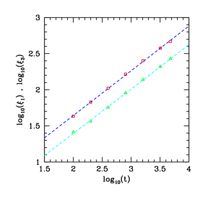
Figure 1: (Color online) Correlation lengths $\xi_{1}$ (squares) and $\xi_{3}$ (triangles) as a function of time for the etching model in $2+1$ dimensions. Dashed lines are least squares fits of each set of data points, respectively with slopes $0.618$ and $0.613$.

III Local roughness distributions in $1+1$ dimensions

III.1 Simulation results for the RSOS model

The expected scaling of RDs foltin ; racz can be extended to LRDs as

$$P_{r}\left(w_{2}\right)=\frac{1}{\langle w_{2}\rangle}\Psi\left(\frac{w_{2}}{\langle w_{2}\rangle}\right).$$ (4)

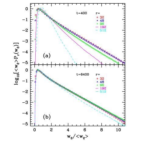
Figure 2: (Color online) Scaled LRDs of the RSOS model in $d=1$ for the listed box sizes at (a) $t=400$ and (b) $t=6400$.

Figs. 2a and 2b shows LRDs of the RSOS model in five box sizes at $t=400$ and $t=6400$, respectively, scaled according Eq. (4). Those plots show that scaled LRDs collapse in certain ranges of $r$. The range begins in $r\sim 30$ and ends at a value that depends on time. At $t=400$ (Fig. 2a), the collapse of curves with $r=32$ and $r=48$ is observed, but there are large discrepancies with the curves of larger $r$. At $t=6400$ (Fig. 2b), good data collapse in two orders of $P\left(w_{2}\right)$ is observed up to $r=192$, with small deviations appearing for smaller $P\left(w_{2}\right)$. A significant deviation is observed only for $r=512$.

When LRDs measured in different growth times are compared, differences between the apparently universal curves of short and long times are also observed. This is observed in Figs. 2a,b, which have the same ranges in both axis: the tail of the collapsed curves at $t=400$ ($r=32$ and $48$) is slightly steeper than the tail of the collapsed curves at $t=6400$ ($r=32$, $48$, and $96$). In linear-linear plots (not shown), it is observed that the scaled LRDs at $t=400$ also have smaller peaks. Thus, the collapse observed in Fig. 2a for small $r$ and short time is not suitable for a quantitative characterization of the universal LRD, although it may be viewed as an anticipation of the existence of a universal distribution (as proposed in Ref. thereza for $d=2$). On the other hand, for $t=6400$ and $t=25600$, good collapse in five orders of magnitude of $P\left(w_{2}\right)$ is observed, indicating a convergence to the universal LRD.

As $r$ increases, Figs. 2a,b shows that the scaled LRD becomes narrower. This corresponds to a decrease in the variation coefficient

$$C\equiv\frac{\sigma}{\langle w_{2}\rangle},$$ (5)

where

$$\sigma\equiv{\left({\langle{w_{2}}^{2}\rangle}-{\langle w_{2}\rangle}^{2}\right)}^{1/2}.$$ (6)

Fig. 3a shows $C$ as a function of $r$ for several times. At the longest times, it shows the formation of plateaus of $C$ in certain ranges of $r$, which is characteristic of a universal (box size independent) LRD. For $t=400$, the two curves that collapsed in Fig. 2a had $C$ between $0.75$ and $0.81$, which are significantly smaller than the values of the long-time plateaus. For $t=1600$, the range $16\leq r\leq 64$ gives a plateau with $C=0.84\pm 0.01$. Results for longer times show wider plateaus with slightly larger values of $C$. Careful inspection of Fig. 3a shows that finite-time corrections appear even when data for $t=12800$ and $t=25600$ are compared. For $t=25600$, $C=0.87\pm 0.01$ is obtained in more than one decade or $r$.

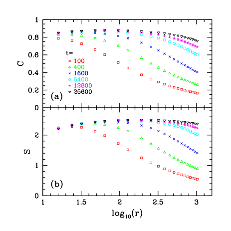
Figure 3: (Color online) (a) Variation coefficient and (b) skewness of the LRDs of the RSOS model in $d=1$ as a function of box size at the listed times.

The LRDs also get a more symmetric shape as $r$ increases. This is related to a decrease of the skewness of the distribution, which is defined as

$$S\equiv\frac{\langle{\left(w_{2}-\langle w_{2}\rangle\right)}^{3}\rangle}{{\langle{\left(w_{2}-\langle w_{2}\rangle\right)}^{2}\rangle}^{3/2}}.$$ (7)

Fig. 3b shows $S$ as a function of $r$ for several times. The presence of plateaus is also observed in those plots, but they are smaller and shifted to larger values of $r$ when compared to the plateaus of $C$ (Fig. 3a). This feature reduces the range of $r$ with constant $C$ and $S$, which is the range of the universal LRD. The values of $S$ in the plateaus also show a non-negligible time dependence: for $t=1600$, an estimate $S=2.36\pm 0.06$ for the universal LRD is suggested; however, for $t=25600$, the plateau formed at larger box sizes gives $S=2.49\pm 0.01$.

For each time, maximal values $C_{max}\left(t\right)$ and $S_{max}\left(t\right)$ were obtained, typically in the middle of the above mentioned plateaus. They were plotted as a function of $t^{-\lambda_{C}}$ and $t^{-\lambda_{S}}$, respectively, for several values of exponents $\lambda_{C}$ and $\lambda_{S}$. For $t\geq 1600$, the exponents that provided the best linear fits of each set of data were $\lambda_{C}=0.35$ and $\lambda_{S}=0.25$, as shown in Figs. 4a,b. Those fits provide extrapolated estimates ($t\to\infty$) $C_{max}=0.896\pm 0.05$ and $S_{max}=2.57\pm 0.02$.

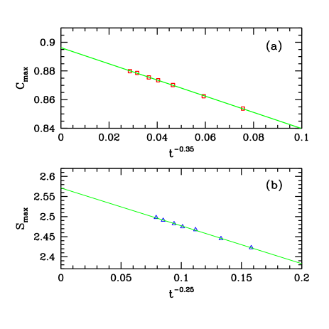
Figure 4: (Color online) Extrapolation in time of the maximal variation coefficient (a) and skewness (b) of the LRDs of the RSOS model in $d=1$. The variables in the abscissa have the exponents that give the best linear fits (solid lines) of each data set.

The fits with small exponents $\lambda_{C}$ and $\lambda_{S}$ are clear indications of large scaling corrections. Estimates of $C$ and $S$ at $t=400$ are almost $10\%$ smaller than the asymptotic ones. Since the RSOS model has relatively weak corrections in the roughness scaling, these results suggest that other models and experimental data may also show large scaling corrections in their LRDs. A comparison of these estimates with analytical results for Gaussian interfaces and with recent numerical data for the KPZ equation is postponed to Sec. III.3.

III.2 Scaling in the box size

Kinetic roughening theory predicts that the height fluctuations of an interface are highly correlated in distances $l\ll\xi$, but uncorrelated at distances $l\gg\xi$. The exact solution of the EW and other linear stochastic equations illustrate this feature ew ; krug .

For this reason, we expect that the scaled LRDs in boxes of sizes $r\ll\xi$ are universal and represent these highly correlated regions. This condition was proposed in Ref. hhpal and was used for choosing LRDs for the comparisons with experimental data in $d=1$ and $d=2$ hhpal ; hhtake . It parallels the universality of the scaled steady state RDs in systems of different lateral sizes $L$, since all wavelengths (up to $\sim L$) are excited in that state foltin ; racz ; antalpre . An additional condition to observe this feature is $r\gg 1$ because this is necessary for a hydrodynamic description to be valid.

On the other hand, when $r\gg\xi\left(t\right)$, a single box is probing a region in which most local heights are uncorrelated. For KPZ in $d=1$, these heights fit to a Tracy-Widom distribution enhanced by a factor that depends on time (as $t^{1/3}$) and on the model, as predicted in Refs. sasamoto ; calabrese and confirmed numerically in Refs. tiagokpz1d2013 ; hhpre2014 . The width of this height distribution is the global roughness at time $t$, $W\left(t\right)$, which has a well defined value for a given KPZ model at a given time. The corresponding LRD is non-zero at a single value $w_{2}={W\left(t\right)}^{2}$, thus the scaled LRD is $\Psi\left(x\right)=\delta\left(x-1\right)$.

This reasoning suggests that that the amplitude ratios which characterize the LRD scale with $r/\xi$. Figs. 5a and 5b show $C$ and $S$, respectively, as a function of $r/\xi_{1}\left(t\right)$. The scaling is confirmed by the good data collapse, with a universal crossover between the stationary LRD and the delta distribution. The time evolution of the maximal values of $C$ and $S$ highlighted in Sec. III.1 (Figs. 4a,b) occurs while the plateaus advance to smaller $r/\xi_{1}$ (left side of Figs. 5a,b). Those plateaus are observed for $r/\xi_{1}\lesssim 0.3$ [$\log{\left(r/\xi_{1}\right)}\leq-0.5$], which is a condition less restrictive than requiring $r\ll\xi$. This is consistent with the time-increasing range of $r$ in which the universal LRD is found.

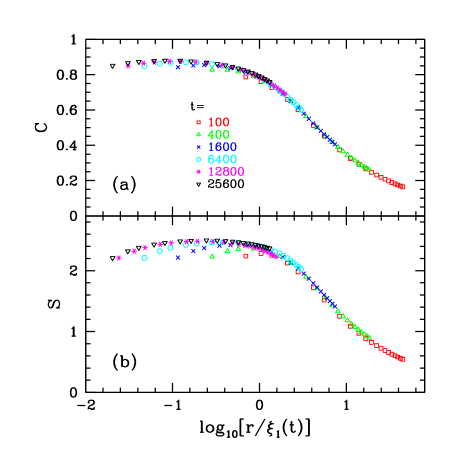
Figure 5: (Color online) (a) Variation coefficient and (b) skewness of the LRDs of the RSOS model in $d=1$ as a function of the scaled box size at the listed times.

A good data collapse is also observed when $C$ and $S$ are plotted as a function of $r/\xi_{3}$ (not shown here). This is expected because $\xi_{1}$ and $\xi_{3}$ scale in time with the same exponent (Sec. II.3). The only change is a small displacement in the range of $r/\xi$ in which the plateaus of $C$ and $S$ are observed.

The convergence of $C$ and $S$ to zero is not shown in Figs. 5a,b because much larger box sizes $r$ would be necessary, requiring simulations in much larger lattices.

III.3 Comparison with steady state and EW distributions

The steady state of the KPZ class in $d=1$ has the same global RD of the EW class foltin . The distribution in periodic boundaries has generating function $G_{PB}\left(x\right)=\sqrt{6x}/\sinh{\sqrt{6x}}$ foltin ; antalpre , with $x\equiv w_{2}/\langle w_{2}\rangle$, which gives $C=\sqrt{2/5}\approx 0.632$ and $S=4\sqrt{10}/7\approx 1.807$. A more relevant comparison is that with distributions of the local roughness in WBC at the steady state by Antal et al antalpre , which are obtained in boxes of size $r\ll L$. The generating function is $G_{WBC}\left(x\right)=\sqrt{\sqrt{12x}/\sinh{\sqrt{12x}}}$ antalpre , which gives $C=2/\sqrt{5}\approx 0.894$ and $S=8\sqrt{5}/7\approx 2.556$. This distribution differs from the global one. We confirmed these estimates by performing simulations of the RSOS model in the steady state.

Ref. hhtake showed the data collapse of KPZ LRDs in the growth regime and the distrubution of Antal et al in WBC. The agreement was also supported by the estimate of the skewness $2.55$ in a plateau in the range of box size $16\leq r\leq 96$. These results suggest that the KPZ nonlinearity does not affect the universal LRDs in the growth regime. Estimates of $C$ were not presented in that work; estimates of the kurtosis varied with $r$, but the accuracy of higher moments of numerically calculated distributions are actually expected to be lower.

Our long time (extrapolated) estimates of $C_{max}$ and $S_{max}$ also agree with the values of Antal et al in the steady state WBC antalpre , confirming the proposal of Ref. hhtake . However, as shown in Sec. III.1, these estimates are obtained in the RSOS model after accounting for large scaling corrections; instead, the plateaus of $C$ and $S$ at the longest simulated time ($t=25600$) are differ from the values of Antal et al antalpre .

The Family model is in the EW class and also has small corrections in the scaling of the average roughness. However, the convergence of the LRDs of this model is even slower than that of the RSOS model. Figs. 6a,b show $C$ and $S$ for the LRD of the Family model. Until $t\sim{10}^{4}$, both quantities are monotonically decreasing with $r$. At $t={10}^{4}$, the linear fit of the $C$ and $S$ data with $32\leq r\leq 128$ has a very small slope; at $t=2\times{10}^{4}$, the slope of this fit is even smaller; this evolution suggests that plateaus will be formed at longer times with $0.88\geq C\geq 0.92$ and $2.5\leq S\leq 2.7$. These values are consistent with the steady state ones of Antal et al antalpre . However, a systematic extrapolation to $t\to\infty$ cannot be performed with this model data, thus these estimates may be viewed only as a guess based on the apparent trends at long times.

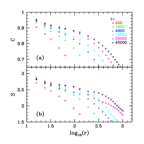
Figure 6: (Color online) (a) Variation coefficient and (b) skewness of the LRDs of the Family model in $d=1$ as a function of the box size at the listed times.

The global RD of an EW interface calculated in Ref. antal96 has vanishing width ($C\to 0$) at times $t$ much smaller than the time of relaxation to the steady state. This is the case of the growth regime studied here. It is consistent with our results because the global RD is measured in $r=L\gg\xi$, supporting the extension of our scaling arguments to other growth classes.

III.4 Distributions scaled by the variance

When steady state RDs are calculated, they are frequently scaled by the variance according to the relation

$$P\left(w_{2}\right)=\frac{1}{\sigma}\Phi\left(\frac{w_{2}-\langle w_{2}\rangle}{\sigma}\right).$$ (8)

The function $\Phi$ is advantageous over $\Psi$ [Eq. (4)] for reducing finite-size effects in numerical data intrinsic . For this reason, scaling by the variance was formerly used with LRDs thereza ; renanPRB ; renanEPL ; hhpal ; hhtake .

However, the function $\Phi$ has unit variance, while the variance of the function $\Psi$ is $C^{2}$. Thus, the crossover features of the relative width $C$ are hidden by Eq. (8). Since estimates of $C$ are typically more accurate than those of $S$ or of the kurtosis, relevant information may be lost in scaling by the variance.

This is confirmed in Figs. 7a,b, which show the same LRDs of Figs. 2a,b scaled by the variance. For $t=400$, deviations from the universal LRD for large $r$ are less striking in Fig. 7a when compared to Fig. 2a. For $t=6400$, the peaks and the right tails for $r\leq 512$ show good collapse in scaling by the variance (Figs. 7b); instead, scaling by the average (Fig. 2b) highlights the deviations for the largest $r$.

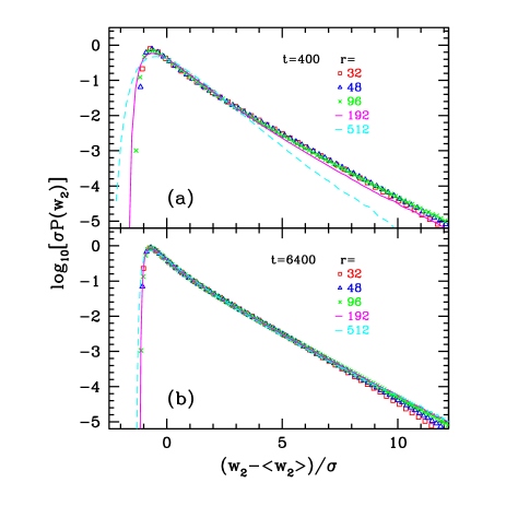
Figure 7: (Color online) LRDs of the RSOS model in $d=1$ scaled by the variance at (a) t=400 and (b) t=6400, for the same box sizes of of Figs. 2a,b.

With scaling by the variance, the differences between the scaled distributions are quantitatively measured by the skewness $S$ or by dimensionless ratios of higher order moments, such as the kurtosis calculated in Refs. thereza ; renanPRB ; renanEPL ; hhpal ; hhtake . However, their accuracy is usually smaller than that of the variation coefficient $C$. Note that this is a particular feature of the LRDs in the growth regime because there is a crossover in the shape of the distribution at $r/\xi\sim 1$.

IV Local roughness distributions in $2+1$ dimensions

IV.1 KPZ class

The collapse of LRDs of the etching and RSOS models was illustrated in Ref. thereza , which was the basis to argue that there is a universal distribution of the KPZ class. In that work, the skewness $S$ and kurtosis $Q$ of the LRDs were also extrapolated to $r\to\infty$ in order to charatectize them in the hydrodynamic limit. Similar procedure was adopted in Refs. renanPRB ; renanEPL .

However, Ref. hhpal argues that this extrapolation is not reliable since the condition $r\ll\xi$ fails for large $r$. This is consistent with the discussion of Sec. III.2, which shows that $C$ and $S$ decrease to zero for very large $r$ (the same occurs with $Q$). For this reason, here we emphasize the scaling of $C$ and $S$ on $r/\xi$ to determine the universal (stationary; small $r$) LRD and its crossover features.

Figs. 8a,b show $C$ and $S$ of the LRDs of the RSOS model as a function of the scaled box size $r/\xi_{1}$. The data collapse confirms the scaling proposed in Sec. III.2, although a tiny time-dependence of the height of the plateaus indicates the presence of scaling corretions. The decrease of $C$ and $S$ for large $r/\xi_{1}$ confirms the convergence of the LRD to a Dirac delta function. The plateaus of $C$ and $S$ in Figs. 8a,b for the longest time ($t=12800$) give estimates $0.49\leq C\leq 0.51$ and $1.97\leq S\leq 2.10$ for the universal LRD.

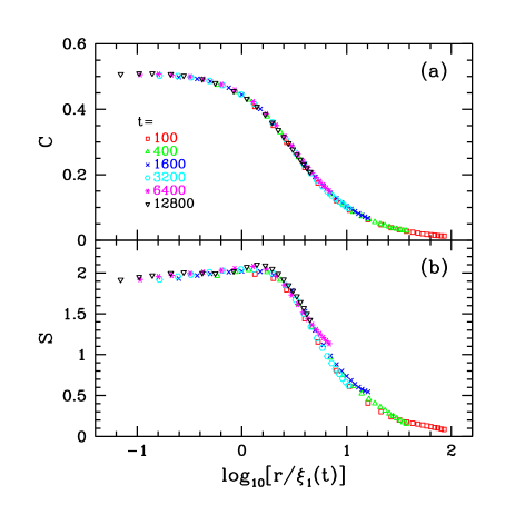
Figure 8: (Color online) (a) Variation coefficient and (b) skewness of the LRDs of the RSOS model in $d=2$ as a function of the scaled box size at the listed times.

However, accounting for finite-time corrections is essential, similarly to the one-dimensional model. The maximal values $C_{max}\left(t\right)$ and $S_{max}\left(t\right)$ are obtained for several times and plotted as a function of $t^{-\lambda_{C}}$ and $t^{-\lambda_{S}}$ for several values of these exponents. In Fig. 9a, we show the extrapolation of $C_{max}$ with $\lambda_{C}=0.25$, which provides the best linear fit of the data for $t\geq 200$. Our asymptotic estimate is $C=0.53\pm 0.02$, which is larger than that predicted in the longest simulated time. On the other hand, Fig. 9b shows a non-monotonic evolution of $S_{max}$. The exponent $\lambda_{S}=0.5$ was used because it fits the data for the longest times, but it is difficult to know wether $S$ will converge with this scaling corrections or will oscillate at longer times. In any case, the evolution of the data in Fig. 9b suggests that the asymptotic $S$ is between $2.0$ and $2.2$.

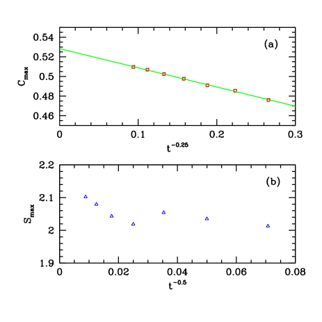
Figure 9: (Color online) Extrapolation in time of the maximal variation coefficient (a) and skewness (b) of the LRDs of the RSOS model in $d=2$. The variable in the abscissa in (a) has the exponent that gives the best linear fit (solid line) of the data.

The estimate of $S$ in Ref. thereza is below this range due to finite-time corrections that were not considered in that work. The estimate $S=2.03$ of Refs. hhpal ; hhtake is included in that range. The study of the time evolution of $C$ seems to improve the comparison of LRDs due to its smaller statistical fluctuations.

Figs. 10a,b show $C$ and $S$ of the LRDs of the etching model. The data is limited to $t\leq 3200$ because flucutations are very large at longer times. In the smallest boxes ($r\leq 32$), deviations from the plateaus of $C$ and $S$ are observed. Those plateaus have larger fluctuations than those of the RSOS model (Figs. 8a,b), but they are consistent with the ranges of $C$ and $S$ presented above.

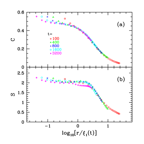
Figure 10: (Color online) (a) Variation coefficient and (b) skewness of the LRDs of the etching model in $d=2$ as a function of the scaled box size at the listed times.

The etching model also has small corrections in the global roughness scaling when compared to most KPZ models kpz2d . Thus, the large fluctuations and significant time-dependence shown in Figs. 10a,b suggest that comparison of LRDs of more complex models or of thin film surfaces may also have large scaling corrections.

A direct comparison of scaled data for the RSOS and the etching models is not shown due to the arbitrariness in the calculation of the correlation length $\xi_{1}$. The collapsed data in Figs. 10a,b are slightly shifted to the right in comparison with the data in Figs. 8a,b.

The above results also show that the condition $r\ll\xi$ proposed in Ref. hhpal may be very restrictive. The plateaus of $C$ and $S$ of the RSOS model are observed for $\log_{10}{\left(r/\xi_{1}\right)}\lesssim 0.5$, i. e. $r\lesssim 0.3\xi_{1}$, similarly to the case $d=1$. This may be particularly important for working with microscopy images in which the conditions $r\gg 1$ (in number of pixels) and $r\ll\xi$ cannot be simulteneously fulfilled. However, the extrapolations of $C_{max}$ and $S_{max}$ are essential to compare those systems LRDs with theoretical ones.

IV.2 VLDS class

The correlation length of the CRSOS model increases in time very slowly because the exponent $z$ is large, as shown in Sec. II. Thus, a collapse of LRDs is obtained only for small $r$ even at very long times ($t>{10}^{4}$). This is illustrated in Figs. 11a and 11b, with LDRs plotted in linear-linear and log-linear scales, respectively: while data for $r=48$ and $r=64$ collapse, significant deviations appear for $r=192$. The LRD becomes narrow and more symmetric as $r$ increases, as expected.

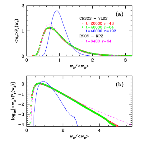
Figure 11: (Color online) Scaled LRDs of the CRSOS model in $d=2$ in (a) linear-linear and (b) log-linear scale at the listed times and box sizes. A scaled LRD of the RSOS model in $d=2$ is also shown for comparison.

A LRD representative of the KPZ class is also shown in Figs. 11a,b. It differs from the CRSOS curves at the peak in the linear plot (Fig. 11a) and at the right tail in the log-linear one (Fig. 11b). However, this occurs because these data have good accuracy; instead, if fluctuations of $10\%$ were present at the peaks and the tails could not be properly sampled (e. g. in the case of a single small microscopy image), then the VLDS and KPZ curves might be indistinguishable. Thus, comparison of LRDs to distinguish universality classes requires good accuracy in the data and independent checks of the distribution peaks (in linear-linear plots) and tails (in log-linear plots).

Figs. 12a,b show $C$ and $S$ of the LRDs of the CRSOS model as a function of $r/\xi_{0}$, confirming the scaling picture of Sec. III.2. These plots do not show plateaus of those quantities, but maximal values $C_{max}\left(t\right)$ and $S_{max}\left(t\right)$ may be extrapolated using the same methods of Secs. III.1 and IV.1. Figs. 13a and 13b show those quantities as a function of $t^{-\lambda_{C}}$ and $t^{-\lambda_{S}}$, respectively, using $\lambda_{C}=0.2$ and $\lambda_{S}=0.35$, which give the best linear fits of each data set for $t\geq 1600$. Asymptotic estimates are $C=0.63\pm 0.06$ and $S=1.58\pm 0.02$.

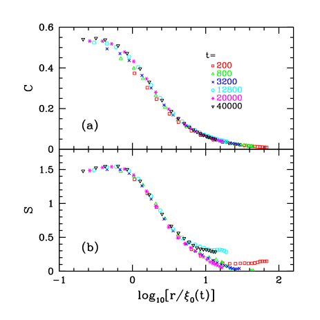
Figure 12: (Color online) (a) Variation coefficient and (b) skewness of the LRDs of the CRSOS model in $d=2$ as a function of the scaled box size at the listed times.

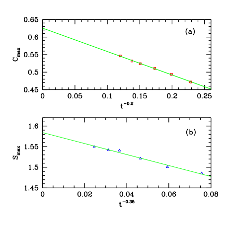
Figure 13: (Color online) Extrapolation in time of the maximal variation coefficient (a) and skewness (b) of the LRDs of the CRSOS model in $d=2$. The variables in the abscissa have the exponents that give the best linear fits (solid lines) of each set of data.

These values are larger than those obtained in the longest simulated time ($t=40000$), which are $C=0.54$ and $S=1.55$. The larger discrepancy in the estimate of $C$ is related to the stronger time dependence or, equivalently, to the smaller correction exponent $\lambda_{C}$. For this reason, using the LRD at $t=40000$ and $r<100$ as representative of the VLDS class may be misleading; for instance, the comparison with the KPZ curve in Fig. 11a shows that they have approximately the same width ($C$), although asymptotic estimates of the two classes differ almost $20\%$.

On the other hand, the skewness of the LRD of the CRSOS model has smaller scaling corrections, which allows us to obtain an asymptotic estimate more accurate than $C$. This skewness is much smaller than that of the KPZ class.

V Conclusion

LRDs in the growth regimes were calcutated in lattice models in the KPZ and VLDS classes in $1+1$ and $2+1$ dimensions. The emphasis on the KPZ LRDs is justified by its theoretical relevance and recent experimental applications.

The LRD is expected to have a universal shape (stationary distribution) if calculated in a range of box size $r$ that satisfies the relation $1\ll r\ll\xi\left(t\right)$, where $\xi\left(t\right)$ is the correlation length, as proposed in previous works. Here, plateaus of the dimensionless ratios $C$ (coefficient of variance) and $S$ (skewness) are observed up to $r\approx 0.3\xi_{1}$, with $\xi_{1}$ defined as the distance in which the autocorrelation function decreases to $10\%$ of its initial value. For $r\gg\xi\left(t\right)$, we argue that the LRD converges to a Dirac delta function. This leads to a universal crossover of those ratios as a function of $r/\xi$, which is confirmed numerically.

The plateaus of $C$ and $S$ are narrow have non-negligible time dependence, even for models that typically have small corrections in the average roughness scaling. Thus, for a reliable quantitative characterization of the universal LRDs, an extrapolation of the maximal values of those ratios is proposed and used to determine their asymptotic values. The consistency of the procedure is confirmed by results for the RSOS model in $1+1$ dimensions, in which the asymptotic estimates of $C$ and $S$ agree with those of steady state EW interfaces in window boundary conditions antalpre . These asymptotic values may differ more than $10\%$ from the plateau values in the maximal simulated times ($\sim{10}^{4}$ layers grown). This shows that accounting for scaling corrections is essential to determine the universality class of a given system by comparison of LRDs.

These results also confirmed the inadequacy of extrapolations of quantities such as $C$ and $S$ to $r\to\infty$, since $r$ may eventually exceed $\xi$ and the LRD will deviate from the universal shape. This was formerly emphasized in Refs. hhpal ; hhtake . Moreover, our results show that scaling by the variance [Eq. (8)] should be avoided because it hinders the changes in $C$. This is usually the most accurate quantity to characterize a distribution calculated numerically, but it was not analyzed in former works on LRDs in the growth regime.

In the CRSOS model, correlations propagate very slowly, thus plateaus of $C$ and $S$ are not observed even at long times. Maximal values were extrapolated in time and provided estimates for the universal LRD. Scaled LRDs of KPZ and VLDS models are visually similar in the usual log-linear scales in two decades, which may turn difficult their use for comparisons with low accuracy data. This reinforces the relevance of the extrapolation procedures.

Comparison of RDs are generally believed to be advantageous over the comparison of height distributions due to the typically small scaling corrections of the steady state distributions. However, the present results show that LRDs in the steady state regime may have large scaling corrections and, consequently, their comparison may not be viewed as a procedure superior to other approaches (e. g. calculation of scaling exponents or height distributions), but as an important additional tool.

Acknowledgements

The author thanks Luis Vázquez for helpful discussion and suggestions to improve the method for comparing local roughness distributions.

This work was supported by CNPq and FAPERJ (Brazilian agencies).

References

References

- (1)
- (2) Barabási A L and Stanley H E 1995 Fractal Concepts in Surface Growth (Cambridge: Cambridge University Press)
- (3) Krug J 1997 Adv. Phys. 46 139
- (4) Halpin-Healy T and Zhang Y C 1995 Phys. Rep. 254, 215
- (5) Evans J W, Thiel P A, and Bartelt M C 2006 Surf. Sci. Rep. 61 1
- (6) Foltin G, Oerding K, Rácz Z, Workman R L, and Zia R K P 1994 Phys. Rev. E 50, R639
- (7) Plischke M, Rácz Z, and Zia R K P 1994 Phys. Rev. E 50, 3589
- (8) Rácz Z and Plischke M 1994 Phys. Rev. E 50, 3530
- (9) Antal T, Droz M, Györgyi G, and Rácz Z 2001 Phys. Rev. Lett. 87, 240601
- (10) Antal T, Droz M, Györgyi G, and Rácz Z 2002 Phys. Rev. E 65, 046140
- (11) Bramwell S T, Christensen K, Fortin J Y, Holdsworth P C W, Jensen H J, Lise S, López J M, Nicodemi M, Pinton J F, and Sellitto M 2000 Phys. Rev. Lett. 84, 3744
- (12) Moulinet S, Rosso A, Krauth W, and Rolley E 2003 Phys. Rev. E 68, 036128
- (13) Edwards S F and Wilkinson D R 1982 Proc. R. Soc. London Ser. A 381 17
- (14) Antal T and Rácz Z 1996 Phys. Rev. E 54, 2256
- (15) Kardar M, Parisi G and Zhang Y C 1986 Phys. Rev. Lett. 56 889
- (16) Villain J 1991 J. Phys. I 1 19
- (17) Lai Z W and Das Sarma S 1991 Phys. Rev. Lett. 66 2348
- (18) Marinari E, Pagnani A, Parisi G, and Rácz Z 2002 Phys. Rev. E 65, 026136
- (19) Aarão Reis F D A 2005 Phys. Rev. E 72, 032601
- (20) Kelling J and Ódor G 2011 Phys. Rev. E 84, 061150
- (21) Paiva T and Aarão Reis F D A 2007 Surf. Sci. 601, 419
- (22) Almeida R A L, Ferreira S O, Oliveira T J, and Aarão Reis F D A 2014 Phys. Rev. B 89, 045309
- (23) Almeida R A L, Ferreira S O, Ribeiro, I R B, and Oliveira T J 2015 EPL 109, 46003
- (24) Halpin-Healy T and Palasantzas G 2014 EPL 105, 50001
- (25) Halpin-Healy T and Takeuchi K A 2015 J. Stat. Phys. 160, 794
- (26) You S and Wan M P 2014 Langmuir 30, 6808
- (27) Kim J M and Kosterlitz J M 1989 Phys. Rev. Lett. 62, 2289
- (28) Mello B A, Chaves A S, and Oliveira F A 2001 Phys. Rev. E 63, 41113
- (29) Family F 1986 J. Phys. A: Math. Gen. 19, L441
- (30) Reis F D A A, 2004 Phys. Rev. E 70 031607
- (31) Kim Y, Park D K, and Kim J M 1994 J. Phys. A: Math. Gen. 27, L533
- (32) Siniscalco D, Edely M, Bardeau J F and Delorme N 2013 Langmuir 29 717
- (33) Aarão Reis F D A 2004 Phys. Rev. E 69, 021610
- (34) Sasamoto T and Spohn H 2010 Phys. Rev. Lett. 104 230602
- (35) Calabrese P and Doussal P L 2011 Phys. Rev. Lett. 106 250603
- (36) Alves S G, Oliveira T J, and Ferreira S C 2013 J. Stat. Mech. P05007
- (37) Halpin-Healy T and Lin T 2014 Phys. Rev. E 89, 010103(R)
- (38) Oliveira T J and Aarão Reis F D A 2007 Phys. Rev. E 76, 061601