Efficient Functional-Based Adaptation for CFD Applications

Abstract

Adjoint methods have gained popularity in recent years for driving adaptation procedures which aim to reduce error in solution functionals. While adjoint methods have been proven effective for functional-based adaptation, the practical implementation of an adjoint method can be quite burdensome since code developers constantly need to ensure and maintain a dual consistent discretization as updates are made. Also, since most engineering problems consider multiple functionals, an adjoint solution must be obtained for each functional of interest which can increase the overall computational cost significantly. In this paper, an alternative to adjoints is presented which uses a sparse approximate inverse of the Jacobian of the residual to obtain approximate adjoint sensitivities for functional-based adaptation indicators. Since the approximate inverse need only be computed once, it can be recycled for any number of functionals making the new approach more efficient than a conventional adjoint method. This new method for functional-based adaptation will be tested using the quasi-1D nozzle problem, and results are presented for functionals of integrated pressure and entropy.

1 Introduction

With the onset of modern computing, computational fluid dynamics (CFD) has become an integral part of both engineering design and analysis. In its short history, CFD has proven to be a very powerful tool in the development and optimization of engineering devices. Although it can offer a tremendous amount of insight into the flow physics governing a particular problem, there will always be some amount of error inherent in CFD simulations due to the required discretization of the governing equations. The presence of this inherent error can be easily forgotten if CFD simulations are viewed as “truth” rather than as an approximation of the true physics. Also, as engineers attempt to optimize their designs to balance performance, efficiency, and cost, the success or failure of their device can hinge on the accuracy of a simulation. Therefore, it is becoming increasingly more important to be able to accurately assess and reduce the numerical error that is present in CFD simulations.

Numerical error is introduced into a simulation through various aspects of the solution procedure such as the chosen discretization scheme and geometry definition. Errors are typically categorized as one of the following: round-off error, iterative error, or discretization error. Round-off error and iterative error are generally not the leading contributors to the overall error in a solution. Due to the increased precision modern computers, round-off error is usually small enough to be neglected. Iterative error will also be small enough to be nglected as long as numerical solutions are fully converged. Discretization error, which is the difference between the exact solution to the discrete governing equations and the exact solution to the continuous governing equations, is often the primary source of numerical error. Accurately assessing the amount of discretization error in a solution can be a very difficult problem; while the discrete numerical solution can serve as the exact solution to the discrete equations to within round-off and iterative error, the exact solution to the continuous governing equations is rarely known. As a result, much research has been conducted to develop methods which can accurately estimate discretization error [1], the most common of which are mesh refinement and residual-based methods.

Mesh refinement methods for discretization error estimation, such as Richardson extrapolation [2], require numerical solutions on multiple grid levels in order to obtain a discretization error estimate. Since only the numerical solution is needed, implementation of a mesh refinement method is straightforward and requires minimal code modifications to produce an error estimate. While implementation may be relatively cheap, a major requirement for these methods is that all grid levels used in obtaining an error estimate must be in the asymptotic range [1]. For a solution to be in the asymptotic range, the mesh resolution must be fine enough such that all higher order terms are small and the discretization error converges at the formal order of accuracy of the discretization. Obtaining solutions in the asymptotic range can be quite difficult especially for nonsmooth problems. Increasing the resolution of the grid uniformly everywhere in order to achieve the asymptotic range can become very computationally expensive. When simulations can sometimes take days or even weeks to run for large, 3D engineering problems, mesh refinement methods for discretization error estimation can quickly become impractical.

Residual-based methods were developed as a cheaper alternative to mesh refinement methods. With a residual-based method, the numerical solution from just one grid level can be used in conjuction with the residual to formulate a discretization error estimate. The reliability of these types of discretization error estimators is heavily dependent upon accurately representing the truncation error, which is the difference between the continuous governing equations and the discrete governing equations operating on the same solution. For complex partial differential equations, deriving an analytic representation of the truncation error, if possible, is a very time-consuming and error-prone process. A numerical truncation error representation is usually constructed in practice. Phillips et al. [3] have had much success numerically estimating truncation error for manufactured solutions to the Euler equations. Once the truncation error is determined, an estimate of discretization error can be established everywhere in the domain.

Equally important to assessing the amount of error in a solution is being able to reduce it. Discretization error can be reduced with uniform grid refinement, but, due to the exponential increase in computational cost, is generally not a viable option for large engineering problems. For instance, in 3D, the computational cost increases on the order of r³ where r is the grid refinement factor. Adaptation, on the other hand, provides an efficient mechanism for increasing solution accuracy without exponentially increasing computation time. Prior to conducting adaptation, two choices must be made which will dictate the performance of the adaptation process: 1) the adaptation indicator and 2) the type of adaptation. The adaptation indicator acts as a flag to target particular cells where adaptation needs to be performed and is used to drive the chosen type of adaptation.

The selection of an appropriate adaptation indicator is the primary factor governing how the adaptation behaves and ultimately the extent to which discretization error will be reduced. Feature-based adaptation flags cells for adaptation based upon the gradient or curvature of one or more flowfield variables making it attractive for resolving shocks and other discontinuous flow features. While feature-based adaptation can provide sharp resolution of discontinuities, this type of adaptation is not guaranteed to reduce numerical errors and can even introduce more error into the solution [4, 5] because it does not account for how discretization error is generated, transported, and dissipated. Rather, feature-based adaptation assumes that error is localized at the feature which may not necessarily be the case. This heuristic approach to adaptation can lead to under-resolution in areas of the domain which contribute most to the discretization error and over-resolution in areas which contribute very little. Truncation error based adaptation seeks to remedy this deficiency on the part of feature-based adaptation. Truncation error, which will be presented in a later section, acts as the local source of discretization error in numerical solutions [6, 7]. By targeting regions of the domain with high truncation error, the local production of discretization error can be reduced. Choudhary and Roy [8] have had success applying this type of adaptation to 1D and 2D Burgers equation. Tyson et al.[9] extended their work in 2D to investigate the application of different adaptation schemes for truncation error based adaptation and were able to achieve substantial reductions in discretization error equivalent to three levels of uniform refinement. While truncation error based adaptation does target the local source of discretization error, like feature-based adaptation, it does not account for how discretization error is transported and diffused throughout the domain.

Adjoint methods have emerged as the state of the art for adaptation which aims to increase the accuracy of a discrete solution functional. These methods have gained popularity due to their rigorous mathematical foundation and because the solution to the adjoint, or dual, problem can also be used to formulate an error estimate in the functional of interest. Adjoint-based adaptation targets areas of the domain which contribute to the overall error in the functional. Venditti and Darmofal [10] applied adjoint methods to quasi-1D flows using an embedded grid technique where a reconstructed coarse grid solution was restricted to an embedded fine grid. In this way, they were able to obtain an error estimate in the solution functional on a fine grid using a coarse grid solution. The solution to the adjoint problem was then used to adapt the coarse grid to obtain a better error estimate on the fine grid. Venditti and Darmofal have also had much success extending their work to 2D inviscid and viscous flows [11, 12]. While adjoint methods have shown great promise for both error estimation and adaptation, the solution to the adjoint problem only supplies an error estimate and adaptivity information for one functional. Typically, engineers require information about multiple functionals such as three forces and three moments for 3D aerodynamics problems. Derlaga [13] was able to circumvent this issue for functional error estimation by showing that local residual-based error estimates can provide the same functional error estimate as an adjoint solution when the same linearization and truncation error estimate are used. This allows error estimates for multiple functionals to be obtained at little to no cost compared to an adjoint method. But, for functional-based adaptation, Park et al. [14] and Fidkowski and Roe [15] have found that adaptation based solely on the adjoint solution for one functional can actually increase the error in another functional. Therefore, for functional-based adaptation, it is still necessary to solve multiple adjoint problems in order to improve all functionals of interest. Solving multiple adjoint problems can become quite costly as the number of functionals increases both in terms of storage and computational time. This could ultimately hinder the widespread use of adjoint methods in commercial applications.

Since most engineering design choices are based upon a given functional of the solution, it is imperative that methods for obtaining functional error estimates and adaptivity information be not only accurate but also efficient. In this paper, we seek an efficient alternative to adjoint methods for functional-based adaptation. First, we will present the relationship between truncation error and discretization error. Adjoint methods for error estimation and adaptation will be reviewed followed by our proposed alternative to adjoints for functional-based adaptation. The new method for functional-based adaptation will be tested using the quasi-1D Euler equations, and adaptation indicators will be compared with those generated by a conventional adjoint solution. Adaptation will be performed and functional discretization error improvements for both methods will be presented.

2 Truncation Error & Discretization Error

2.1 Generalized Truncation Error Expression

Before the relationship between truncation error and discretization error can be presented, the relationship between the continuous form and the discrete form of the governing equations must be understood. A given set of continuous governing equations, $L(\cdot)$, may be related to a consistent discretized form of the equations, $L_{h}(\cdot)$, by the Generalized Truncation Error Expression (GTEE) [7]:

$$L_{h}(I^{h}u)=I^{h}L(u)+\tau_{h}(u)$$ (1)

where $u$ is any continuous function and $\tau_{h}(\cdot)$ represents the truncation error. From Eq. 1, it can be seen that the truncation error, as the difference between the continuous and discrete forms of the governing equations, represents higher order terms which are truncated in the discretization process. For model problems, the truncation error can be shown to be a function of continuous solution derivatives and cell size [16]. But, while operating on a continuous solution space, evaluating the truncation error results in a discrete space [3, 17]. The operator, $I_{a}^{b}$, is a restriction or prolongation operator which allows for the transition between a continuous space and a discrete space; the subscript, $a$, denotes the starting space and the superscript, $b$, denotes the resultant space. For the GTEE, a subscript or superscript $h$ denotes a discrete space on a mesh with a characteristic size, $h$, and an empty subscript or superscript represents a continuous space. Also, there is no restriction on the form of the continuous and discrete operators, $L(\cdot)$ and $L_{h}(\cdot)$; the governing equations can be strong form (ODEs and PDEs) or weak form (integral equations).

2.2 Error Transport Equations

Having related the contiuous governing equations, $L(\cdot)$, to the discrete governing equations, $L_{h}(\cdot)$, through the truncation error, $\tau_{h}(\cdot)$, we are now in a position to relate truncation error to the discretization error. First, consider the following definitions. For the exact solution to the continuous governing equations, $\tilde{u}$, and the exact solution to the discrete governing equations, $u_{h}$, the following holds:

$$L(\tilde{u}) =0$$ (2a)

$$L_{h}(u_{h}) =0$$ (2b)

Plugging the exact solution to the discrete equations, $u_{h}$, into the GTEE and noting that the left hand side is identically zero by Eq. 2b, the GTEE may be simplified to the following:

$$0=I^{h}L(I_{h}u_{h})+\tau_{h}(I_{h}u_{h})$$ (3)

where $I_{h}$ prolongs the exact discrete solution to a continuous space. Next, the continuous governing equations, Eq. 2a, can be subtracted from both sides of Eq. 3 to form:

$$0=I^{h}L(I_{h}u_{h})-I^{h}L(\tilde{u})+\tau_{h}(I_{h}u_{h})$$ (4)

Finally, if we define the discretization error as the difference between the exact solution to the discrete equations and the exact solution to the continuous equations, $I_{h}\varepsilon_{h}=I_{h}u_{h}-\tilde{u}$, and if the governing equations are linear or linearized [17, 7], the continuous operators in Eq. 4 can be combined and the definition of discretization error may be inserted to form the continuous form of the error transport equations (ETE):

$$I^{h}L(I_{h}\varepsilon_{h})=-\tau_{h}(I_{h}u_{h})$$ (5)

An equivalent discrete form of the ETE can also be derived and are given by:

$$L_{h}(\varepsilon_{h})=-\tau_{h}(\tilde{u})$$ (6)

The ETE provide a great deal of information regarding how discretization error behaves and how it is related to the truncation error. Eq. 5 and Eq. 6 demonstrate that truncation error acts as the local source for discretization error in numerical solutions and that discretization error is convected and diffused in the same manner as the solution.

2.3 Truncation Error Estimation

In practice, the discrete form of the ETE, Eq. 6, are used to solve for the local discretization error throughout the domain. But in order to do this, the exact solution to the continuous equations, $\tilde{u}$, must be known to evaluate the truncation error. Since the exact continuous solution is in practice never known, the truncation error is typically estimated with a reconstruction of the discrete solution, that is:

$$\tau_{h}(\tilde{u})\approx\tau_{h}(I_{h}^{q}u_{h})$$ (7)

where $I_{h}^{q}u_{h}$ is a $q^{th}$-order reconstruction of the exact discrete solution, $u_{h}$. The discrete numerical solution is often a very good approximation of the exact discrete solution, $u_{h}$, assuming round-off and iterative errors are small. To estimate the truncation error, the exact solution to the discrete equations is inserted into Eq. 1 such that [3]:

$$\tau_{h}(I_{h}^{q}u_{h})=-I^{h}L(I_{h}^{q}u_{h})+O(h^{\bar{q}})$$ (8)

where $\bar{q}$ is an order similar to $q$ but altered by the continuous govering equations, $L(\cdot)$. Therefore, operating the continuous residual, $L(\cdot)$, on the reconstructed solution provides the necessary truncation error estimate for solving the ETE.

3 Functional-Based Adaptation

3.1 Adjoint Methods

While adjoint methods were originally used in design optimization to obtain sensitivities of a functional to a set of design parameters [18], adjoint methods have gained much popularity within the CFD community for obtaining functional error estimates and adaptation indicators. Solutions from the adjoint, or dual, problem can be used to drive an adaptation procedure which only targets regions of the domain which contribute to the discretization error in the functional of interest. In order to illustrate why adjoint methods can be used in this way, first consider a Taylor expansion of the discrete equations, $L_{h}(u_{h})$, about a general discrete function, $u$:

$$L_{h}(u_{h})=L_{h}(u)+\frac{\partial L_{h}}{\partial U}\bigg{|}_{U=u}(u_{h}-u)+\frac{\partial^{2}L_{h}}{\partial U^{2}}\bigg{|}_{U=u}\frac{(u_{h}-u)^{2}}{2}+\ldots$$ (9)

Likewise, consider a similar expansion of a discrete solution functional, $J_{h}$, about the same general discrete function, $u$:

$$J_{h}(u_{h})=J_{h}(u)+\frac{\partial J_{h}}{\partial U}\bigg{|}_{U=u}(u_{h}-u)+\frac{\partial^{2}J_{h}}{\partial U^{2}}\bigg{|}_{U=u}\frac{(u_{h}-u)^{2}}{2}+\ldots$$ (10)

Combining Eq. 9 and Eq. 10 in a Lagrangian, the functional, $J_{h}(\cdot)$, evaluated at the exact discrete solution, $u_{h}$, may be rewritten as:

$$J_{h}(u_{h}) =\left[J_{h}(u)+\frac{\partial J_{h}}{\partial U}\bigg{|}_{U=u}(u_{h}-u)+\frac{\partial^{2}J_{h}}{\partial U^{2}}\bigg{|}_{U=u}\frac{(u_{h}-u)^{2}}{2}+\ldots\right]$$ (11)

$$+ \lambda^{T}\left[L_{h}(u)+\frac{\partial L_{h}}{\partial U}\bigg{|}_{U=u}(u_{h}-u)+\frac{\partial^{2}L_{h}}{\partial U^{2}}\bigg{|}_{U=u}\frac{(u_{h}-u)^{2}}{2}+\ldots\right]$$

where $\lambda^{T}$ is a 1xN vector of Lagrange multipliers where N is the total number of unknowns. This operation is made possible by the fact that the terms in brackets following the Lagrange multipliers, $\lambda$, are exactly equal to zero by Eq. 9 and Eq. 2b. Now, neglecting higher order terms, inserting a restriction of the exact solution to the continuous equations, $I^{h}\tilde{u}$, for the general discrete function, $u$, and using the definition of discretization error, $\varepsilon_{h}=u_{h}-I^{h}\tilde{u}$, Eq. 11 may be simplified to the following:

$$J_{h}(u_{h})\approx J_{h}(I^{h}\tilde{u})+\frac{\partial J_{h}}{\partial U}\bigg{|}_{U=I^{h}\tilde{u}}\varepsilon_{h}+\frac{\partial^{2}J_{h}}{\partial U^{2}}\bigg{|}_{U=I^{h}\tilde{u}}\frac{\varepsilon_{h}^{2}}{2}+\lambda^{T}\left[L_{h}(I^{h}\tilde{u})+\frac{\partial L_{h}}{\partial U}\bigg{|}_{U=I^{h}\tilde{u}}\varepsilon_{h}+\frac{\partial^{2}L_{h}}{\partial U^{2}}\bigg{|}_{U=I^{h}\tilde{u}}\frac{\varepsilon_{h}^{2}}{2}\right]$$ (12)

If the first term on the right hand side is taken to the left hand side and the error in the functional is approximated as $\varepsilon_{J}=J_{h}(u_{h})-J_{h}(I^{h}\tilde{u})$, Eq. 12 becomes analogous to solving a constrained optimization problem which seeks to minimize the error in the functional subject to satisfying the discrete governing equations, $L_{h}(u_{h})=0$. Finally, if the exact solution to the continuous governing equations, $\tilde{u}$, is inserted into the GTEE so that $L_{h}(I^{h}\tilde{u})=\tau_{h}(\tilde{u})$, Eq. 12 may be simplified and rearranged to form:

$$\underbrace{\vphantom{\left[\frac{\partial J_{h}}{\partial U}\bigg{|}_{U=I^{h}\tilde{u}}\right]}J_{h}(u_{h})-J_{h}(I^{h}\tilde{u})}_{\text{Functional Error}}\approx\underbrace{\vphantom{\left[\frac{\partial J_{h}}{\partial U}\bigg{|}_{U=I^{h}\tilde{u}}\right]}\lambda^{T}\tau_{h}(\tilde{u})}_{\text{Correction}}+\varepsilon_{h}\underbrace{\left[\frac{\partial J_{h}}{\partial U}\bigg{|}_{U=I^{h}\tilde{u}}+\lambda^{T}\frac{\partial L_{h}}{\partial U}\bigg{|}_{U=I^{h}\tilde{u}}\right]}_{\text{Adjoint Problem}}+\underbrace{\frac{\varepsilon_{h}^{2}}{2}\left[\frac{\partial^{2}J_{h}}{\partial U^{2}}\bigg{|}_{U=I^{h}\tilde{u}}+\lambda^{T}\frac{\partial^{2}L_{h}}{\partial U^{2}}\bigg{|}_{U=I^{h}\tilde{u}}\right]}_{\text{Remaining Error}}$$ (13)

Eq. 13 represents the discrete adjoint formulation of the functional error. An equivalent continuous formulation can be derived in a similar manner. Before moving forward, it is important to note that from now on the Lagrange multipliers, $\lambda$, will be referred to as the adjoint variables or adjoint sensitivities. The adjoint variables represent the sensitivity of the functional to local perturbations of the residual.

The functional error estimate consists of three parts: (1) the computable adjoint correction, (2) the solution of the adjoint problem, and (3) higher order remaining error terms. The adjoint correction is computed by first solving the adjoint problem such that the terms in brackets are equal to zero:

$$\frac{\partial J_{h}}{\partial U}\bigg{|}_{U=I^{h}\tilde{u}}+\lambda^{T}\frac{\partial L_{h}}{\partial U}\bigg{|}_{U=I^{h}\tilde{u}}=0$$ (14)

Rearranging Eq. 14 yields a system of linear equations for the adjoint variables, $\lambda$:

$$\left[\frac{\partial L_{h}}{\partial U}\bigg{|}_{U=I^{h}\tilde{u}}\right]^{T}\lambda=-\left[\frac{\partial J_{h}}{\partial U}\bigg{|}_{U=I^{h}\tilde{u}}\right]^{T}$$ (15)

It is important to note that the term in brackets on the left hand side of Eq. 15 is the Jacobian of the primal solution which, for a code that includes an implicit solver, will already be computed and stored. Already having computed the Jacobian can make implementation of an adjoint method slightly less challenging. Now, upon inspection of Eq. 15, it can be seen that the adjoint variables represent the discrete sensitivities of the functional to perturbations in the discrete operator making them an ideal candidate for flagging areas of the domain for adaptation which contribute most to error in the chosen functional. Once the adjoint problem has been solved for the adjoint variables, the adjoint correction term may be computed assuming an accurate truncation error estimate has been determined such that Eq. 7 holds. Finally, having solved the adjoint problem and having computed the adjoint correction, all that remains are higher order remaining error terms. These higher order terms can be quite expensive to compute and are most often left unquantified. But, for a second order accurate discretization, while the adjoint correction reduces at a second order rate, the remaining error terms will drop at a fourth order rate. This higher order convergence of the remaining error terms indicates that even for coarse grids the magnitude of the remaining error can be small relative to the adjoint correction.

3.2 Approximate Adjoint Methods

Adjoint methods appear to be ideal for functional-based error estimation and adaptation because of their rigorous mathematical foundation and because both error estimates and adaptation indicators can be obtained in one compact procedure. But, since most engineering problems require analyzing multiple solution functionals, the adjoint problem must be solved for each functional of interest. As the number of required functionals increases, the cost of solving several adjoint problems can become impractical. Research has also shown that adaptation which solely targets one functional can actually increase the error in another functional [14, 15] thus furthering the need to solve the adjoint problem for all functionals of interest. In addition to an increase in computational cost, proper implementation of an adjoint solver can be quite burdensome. The developer must pay careful consideration to maintaining a dual consistent discretization between the primal solver and the adjoint solver so that information is not transported in a manner inconsistent with the physics of the problem. Derlaga et al. [19] offer an example of how a dual inconsistent implementation of boundary conditions can corrupt the adjoint solution.

While adjoint methods have been proven effective for functional error estimation and adaptation, these methods have clear disadvantages which could ultimately prevent their widespread use in commercial applications. In this section, we present an alternative approach to adjoint methods whose sole purpose is to increase the efficiency of functional-based adaptation by alleviating the need to solve an adjoint problem for each functional of interest. To accomplish this, we must first derive the implicit form of the discrete ETE, Eq. 6. By inserting the exact solution to the continuous governing equations, $\tilde{u}$, into the GTEE and subtracting Eq. 2b from both sides, the GTEE can be rewritten as:

$$L_{h}(u_{h})-L_{h}(I^{h}\tilde{u})=-\tau_{h}(\tilde{u})$$ (16)

Next, consider an expansion of the discrete governing equations, $L_{h}(\cdot)$, operating on a restriction of the exact continuous solution, $I^{h}\tilde{u}$, about the exact discrete solution, $u_{h}$:

$$L_{h}(I^{h}\tilde{u})=L_{h}(u_{h})-\frac{\partial L_{h}}{\partial U}\bigg{|}_{U=u_{h}}\varepsilon_{h}+O(\varepsilon_{h}^{2})$$ (17)

Inserting Eq. 17 and Eq. 7 into Eq. 16 and neglecting higher order terms, we arrive at the implicit form of the discrete ETE:

$$\frac{\partial L_{h}}{\partial U}\bigg{|}_{U=u_{h}}\varepsilon_{h}\approx-\tau_{h}(I_{h}^{q}u_{h})$$ (18)

where the $\frac{\partial L_{h}}{\partial U}\bigg{|}_{U=u_{h}}$ is simply the Jacobian for the primal solution which again for a code that implements an implicit primal solver is already available. Now, consider a similar expansion of the functional about the exact solution to the discrete equations, $u_{h}$:

$$J_{h}(I^{h}\tilde{u})=J_{h}(u_{h})+\frac{\partial J_{h}}{\partial U}\bigg{|}_{U=u_{h}}\underbrace{(u_{h}-I^{h}\tilde{u})}_{\varepsilon_{h}}+O(\varepsilon_{h}^{2})$$ (19)

Noting that the term in parenthesis is the definition of discretization error, $\varepsilon_{h}$, and by rearranging and neglecting higher order terms, the error in the functional can be expressed as:

$$\varepsilon_{J}=J_{h}(u_{h})-J_{h}(I^{h}\tilde{u})\approx-\frac{\partial J_{h}}{\partial U}\bigg{|}_{U=u_{h}}\varepsilon_{h}$$ (20)

Solving Eq. 18 for the discretization error, $\varepsilon_{h}$, and inserting into Eq. 20, the error in the functional can be written as the following:

$$\varepsilon_{J}\approx\frac{\partial J_{h}}{\partial U}\bigg{|}_{U=u_{h}}\left[\frac{\partial L_{h}}{\partial U}\bigg{|}_{U=u_{h}}\right]^{-1}\tau_{h}(I_{h}u_{h})$$ (21)

By comparing Eq. 21 with Eq.13, it can be seen that if the Jacobian, $\frac{\partial L_{h}}{\partial U}\bigg{|}_{U=u_{h}}$, is the full second order linearization and if it is inverted exactly then Eq. 21 is identical to an adjoint method where the higher order remaining error terms have been neglected and the adjoint variables, $\lambda$, are given by:

$$\lambda^{T}=\frac{\partial J_{h}}{\partial U}\bigg{|}_{U=u_{h}}\left[\frac{\partial L_{h}}{\partial U}\bigg{|}_{U=u_{h}}\right]^{-1}$$ (22)

For functional error estimation, the Jacobian must be inverted exactly in order to obtain an accurate functional error estimate. In practice, this inversion is too expensive and Eq. 22 is solved using a krylov subspace method such as GMRES [20]. But, for functional-based adaptation, we only require an adaptation indicator which flags areas of the domain for adaptation. Therefore, since the adjoint variables only serve as an indicator, they need not be as accurate as is required for functional error estimation. To approximate the adjoint variables, rather than solve Eq. 22 using an iterative method, the inverse of the Jacobian can instead be replaced with an approximate inverse. This not only saves computational resources, but also allows the inverse of the Jacobian to be recycled for multiple functionals. In this paper, we investigate using sparse approximate inverse preconditioning techniques to generate an approximate inverse of the residual Jacobian [21, 22].

3.3 Grid Adaptation

Grid adaptation is performed using a structured adaptation module (SAM) developed by Choudhary [23] which implements several 1D and 2D r-adaptation schemes. For this study, a center of mass adaptation procedure is used which equidistributes a prescribed weight function across the computational domain. During the equidistribution process, nodes of the mesh are shifted, as illustrated in Fig. 1, in order to make the quantity cell size (i.e. $\Delta x$ in 1D) times weight function equal-valued in all cells of the domain.

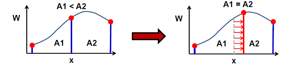
Figure 1: Weight Function Equidistribution [24]

With this type of adaptation, the number of nodes in the mesh remains constant throughout the adaptation process. This can lead to significant computational savings over other forms of adaptation, such as h-adaptation, where the number of nodes in the mesh can increase.

Prior to conducting adaptation, care must be taken to formulate the weight function in a manner which will achieve the desired adaptive behavior. Ideally, it is preferred that resolution is increased in areas of the domain where discretization error is large while decreasing resolution in areas where it is small. But, solely using discretization error to drive adaptation generally tends to not achieve this goal as well as using truncation error to drive the adaptation process [6, 25, 26]. While truncation error can be used to drive adaptation which targets the overall discretization error in a solution, we seek a weight function which adapts cells which contribute to the error in a functional. Derlaga et al. [19, 27] and Derlaga [13] were able to accomplish this by weighting the local truncation error by the adjoint sensitivities and, in some cases, were even able to achieve greater reductions in functional error over other adjoint-based adaptation indicators. In this study, the weight function proposed by Derlaga et al. [19, 27] and Derlaga [13] is used to drive adaptation. This weight function is formulated by normalizing the adjoint-weighted truncation error in cell $i$ on a given mesh, $k$, by the infinity norm of the adjoint-weighted truncation error on the initial mesh and averaging over $N$ governing equations:

$$w_{i}=\frac{1}{N}\sum\limits_{j=1}^{N}\frac{\bigl{\lvert}\lambda_{i,j}\tau_{h}(I_{h}^{q}u_{h})_{i,j}^{k}\bigr{\rvert}}{\bigl{\lvert}\bigl{\lvert}\lambda_{j}\tau_{h}(I_{h}^{q}u_{h})_{j}^{k=1}\bigr{\rvert}\bigr{\rvert}_{\infty}}$$ (23)

4 Test Case

4.1 Quasi-1D Nozzle

The quasi-1D nozzle problem is used to investigate the effectiveness of the proposed alternative to adjoint methods for functional-based adaptation. The nozzle is characterized by a contraction which accelerates the flow to Mach 1 at the throat followed by a diverging section which allows the flow to expand subsonically or supersonically depending upon the pressure at the nozzle exit. Since the quasi-1D nozzle problem has an exact solution, it is the ideal test bed for investigating these new methods for functional-based adaptation.

4.1.1 Geometry & Boundary Conditions

The geometry of the nozzle used in this study is taken from Jackson and Roy [24] and has a gaussian area distribution given by the following:

$$A(x)=1-0.8e^{\left(\frac{-x^{2}}{2\sigma^{2}}\right)},\quad-1\leq x\leq 1$$ (24)

where $\sigma$ is chosen as 0.2. This nozzle geometry was chosen for its lack of curvature discontinuities which can cause spurious truncation error spikes [24] and can make truncation error estimation more diffucult. For this study, only isentropic expansions are examined where the flow in the diverging section is entirely subsonic or supersonic. The area distribution and the Mach number distributions for both subsonic and supersonic isentropic expansions can be seen in Fig. 3. The corresponding pressure distributions throughout the nozzle can be seen in Fig. 3.

At the inflow of the nozzle, the stagnation pressure and temperature are fixed at 300 kPa and 600 K, respectively. The Mach number is extrapolated from the interior to set the inflow state at the face. The outflow boundary conditions depend upon the expansion of the flow in the diverging section of the nozzle. For a supersonic isentropic expansion, all variables in the interior are extrapolated to the face to set the outflow flux. For a subsonic isentropic expansion, a back pressure is set and velocity and density are extrapolated from the interior. The back pressure is set to 297.158 kPa in this study.

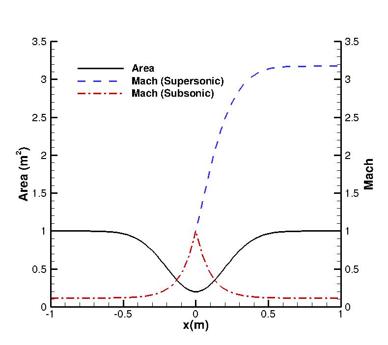
Figure 2: Gaussian Nozzle: Area/Mach Number Distribution

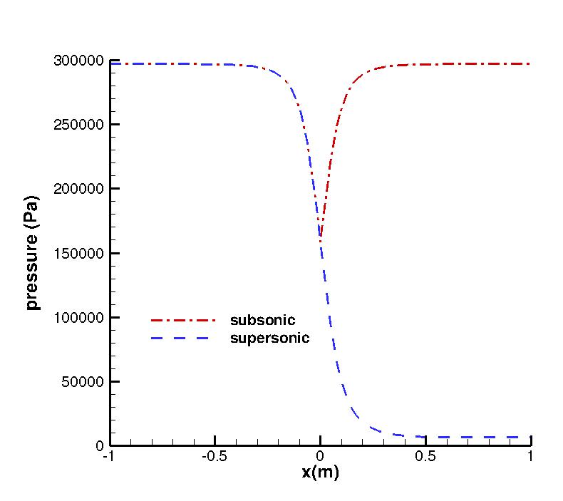
Figure 3: Gaussian Nozzle: Pressure Distribution

4.1.2 Numerical Methods: Finite Volume Discretization

The flow in the nozzle is solved numerically using the quasi-1D form of the Euler equations. The Euler equations in weak, conservation form for a control volume fixed in space take the following generic form:

$$\frac{\partial}{\partial t}\int_{\Omega}\vec{Q}\,d\Omega+\oint_{\partial\Omega}\left(\vec{F}_{i}-\vec{F}_{v}\right)\,dS\ =\int_{\Omega}\vec{S}\,d\Omega$$ (25)

where $\vec{Q}$ is the vector of conserved variables, $\vec{F}_{i}$ is the vector of inviscid fluxes, $\vec{F}_{v}$ is the vector of viscous fluxes, $\vec{S}$ is a generic source term, and $\Omega$ is the control volume over which conservation of mass, momentum, and energy must be satisfied. For the quasi-1D form of the Euler equations, the vector of conserved variables, $\vec{Q}$, the fluxes, $\vec{F}_{i}$ and $\vec{F}_{v}$, and the source term, $\vec{S}$, are given by:

$$\vec{Q}=\begin{bmatrix}\rho\\ \rho u\\ \rho e_{t}\end{bmatrix},\quad\vec{F}_{i}=\begin{bmatrix}\rho u\\ \rho u^{2}+p\\ \rho uh_{t}\end{bmatrix},\quad\vec{F}_{v}=\begin{bmatrix}0\\ 0\\ 0\end{bmatrix},\quad\vec{S}=\begin{bmatrix}0\\ p\frac{dA}{dx}\\ 0\end{bmatrix}$$ (26)

where $\frac{dA}{dx}$ describes how the cross-sectional area of the nozzle changes down its length. The system of equations is closed using the equation of state for a perfect gas such that the total energy, $e_{t}$, and total enthalpy, $h_{t}$, are given by:

$$e_{t}=\frac{p}{\rho(\gamma-1)}+\frac{u^{2}}{2},\quad h_{t}=\frac{\gamma p}{\rho(\gamma-1)}+\frac{u^{2}}{2}$$ (27)

where $\gamma$ is the ratio of specific heats for a perfect gas which for air is $\gamma=1.4$.

The quasi-1D form of the Euler equations, Eqs. 25 and 26, are discretized using a second order, cell-centered finite-volume discretization. The inviscid fluxes are computed using Roe’s flux difference splitting scheme [28] and Van Leer’s flux vector splitting scheme [29]. MUSCL extrapolation [30] is used to reconstruct the fluxes to the face in order to obtain second order spatial accuracy. The boundary conditions are weakly enforced through the fluxes. Numerical solutions are marched in time to a steady-state using an implicit time stepping scheme [31] given by the following:

$$\left[\frac{\Omega}{\Delta t}I+\frac{\partial\vec{R}}{\partial\vec{Q}}\right]^{n}\Delta\vec{Q}^{n}=-\vec{R}^{n}$$ (28)

where $\Omega$ is the volume of a given cell, $\Delta t$ is the time step, $I$ is the identity matrix, $\frac{\partial\vec{R}}{\partial\vec{Q}}$ is the Jacobian matrix, $\Delta\vec{Q}^{n}$ is a forward difference of the conserved variable vector given by $\Delta\vec{Q}^{n}=\vec{Q}^{n+1}-\vec{Q}^{n}$, and $\vec{R}^{n}$ is the residual evaluated at time level $n$. For the code used in this study, only the primitive variables are stored, therefore, a conversion matrix is added to convert the conserved variable vector, $\vec{Q}$, to the primitive variable vector, $\vec{q}$, such that:

$$\left[\frac{\Omega}{\Delta t}\frac{\partial\vec{Q}}{\partial\vec{q}}+\frac{\partial\vec{R}}{\partial\vec{q}}\right]^{n}\Delta\vec{q}^{n}=-\vec{R}^{n}$$ (29)

where $\frac{\partial\vec{Q}}{\partial\vec{q}}$ is the conversion matrix and $\vec{q}$ is the primitive variable vector given by $\vec{q}=\left[\rho,u,p\right]^{T}$. The residual in a given cell, $\vec{R}_{i}$, for the quasi-1D Euler equations is given by:

$$\vec{R}_{i}^{n}=\vec{F}_{i+1/2}^{n}A_{i+1/2}-\vec{F}_{i-1/2}^{n}A_{i-1/2}-\vec{S}_{i}^{n}\Delta x_{i}$$ (30)

where $\vec{F}_{i+1/2}$ and $\vec{F}_{i-1/2}$ are the inviscid fluxes at the faces on each side of cell $i$, $A_{i+1/2}$ and $A_{i-1/2}$ are the corresponding face areas, and $\Delta x_{i}$ is the size of cell $i$. For the primal solver, the Jacobian matrix, $\frac{\partial\vec{R}}{\partial\vec{Q}}$, does not need to be the full second order linearization since the left hand side of Eq. 29 is just used to drive the residual, the right hand side of Eq. 29, to zero. But, to maintain second order spatial accuracy, the residual must be the second order discretization.

The discretization of the adjoint problem is performed using the discretization outlined in [32] and is given by:

$$\left[\frac{\Omega}{\Delta t}\frac{\partial\vec{Q}}{\partial\vec{q}}+\frac{\partial\vec{R}}{\partial\vec{q}}\right]^{T}\Delta\vec{\lambda}^{n}=-\left(\frac{\partial J_{h}}{\partial\vec{q}}+\left[\frac{\partial\vec{R}}{\partial\vec{q}}\right]^{T}\vec{\lambda}^{n}\right)$$ (31)

where $\Delta\vec{\lambda}^{n}$ is a forward difference of the adjoint variables given by $\Delta\vec{\lambda}^{n}=\vec{\lambda}^{n+1}-\vec{\lambda}^{n}$. Similar to the primal solution, the Jacobian on the left hand side of Eq. 31 need not be the full second order linearization. But, in order to obtain a usable adjoint solution, the Jacobian on the right hand side of Eq. 31 is required to be the full second order linearization.

4.1.3 Functionals of Interest

For this study, two discrete solution functionals will be examined. The first functional, the integrated value of pressure along the nozzle, is the same functional used by Venditti and Darmofal [10] for their original work and is given by:

$$J_{h}=\int_{-1}^{1}p(x)dx$$ (32)

The second functional under consideration is the integrated value of entropy along the nozzle examined by Derlaga et al.  [19]:

$$J_{h}=\int_{-1}^{1}\frac{p}{\rho^{\gamma}}dx$$ (33)

5 Progress & Future Work

The use of an adjoint method for functional-based error estimation and adaptation can quickly become too costly when multiple functionals are of interest. Previous work from our research group has shown that local residual-based error estimation can be used as a much cheaper alternative to adjoints when multiple functional error estimates are required since local residual-based error estimates can provide the same functional error estimate as an adjoint method as long as the same linearization and truncation error estimate are used [13]. An example of this from the work of Derlaga [13] may be seen in Fig. 5 and Fig. 5 for a 2D supersonic expansion fan where defect correction (DC), error transport equations (ETE), and adjoints produced essentially the same error estimate for the normal force on the wall. For this paper, we now seek a more efficient method for functional-based adaptation that will alleviate the need for an adjoint method when multiple functionals are required.

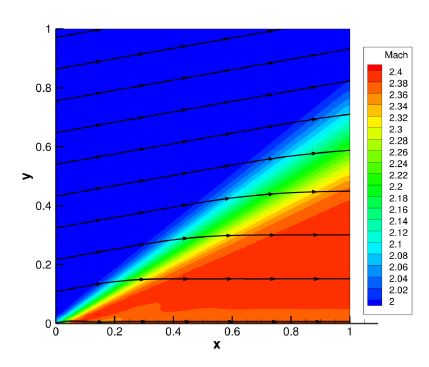
Figure 4: Expansion Fan: Mach Number Distribution [13]

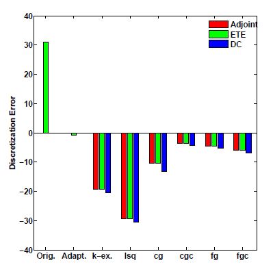
Figure 5: Force Functional Error Estimation [13]

Currently, both the primal solver and dual solver are implemented and running properly for the quasi-1D nozzle problem due to the previous work of Derlaga et al. [19] and Derlaga [13]. The structured adaptation module, SAM, is also implemented and interfaces well with the quasi-1D nozzle code[19, 24]. As far as the solver, minimal changes will need to be made for the work proposed in this paper. Thanks to the hard work of previous developers, implementation of a sparse approximate inverse for the Jacobian of the primal solution should be relatively straightforward. For the final draft of the paper, a sparse approximate inverse will be implemented and weight functions for adaptation will be generated using the methods outlined in this abstract. These weight functions will be compared to those generated using a typical adjoint method to examine the viability of the new approach for functional-based adaptation. The test results will include adaptation for both of the proposed functionals for subsonic and supersonic cases of the quasi-1D nozzle. Functional discretization error improvements will be examined for all test cases using an adjoint method as well as the new, approximate adjoint approach for functional-based adaptation.

References

- [1] Roy, C., “Review of Discretization Error Estimators in Scientific Computing,” 48th AIAA Aerospace Sciences Meeting Including the New Horizons Forum and Aerospace Exposition, Jan 2010.
- [2] Richardson, L. F., “The Approximate Arithmetical Solution by Finite Differences of Physical Problems Involving Differential Equations, with an Application to the Stresses in a Masonry Dam,” Philosophical Transactions of the Royal Society A: Mathematical, Physical and Engineering Sciences, Vol. 210, No. 459-470, Jan 1911, pp. 307–357.
- [3] Phillips, T., Derlaga, J. M., Roy, C. J., and Borggaard, J., “Finite Volume Solution Reconstruction Methods For Truncation Error Estimation,” 21st AIAA Computational Fluid Dynamics Conference, Jun 2013.
- [4] Warren, G., Anderson, W., Thomas, J., and Krist, S., “Grid convergence for adaptive methods,” 10th Computational Fluid Dynamics Conference, Jun 1991.
- [5] Ainsworth, M. and Oden, J., A Posteriori Error Estimation in Finite Element Analysis, Wiley Interscience, New York, 2000.
- [6] Roy, C., “Strategies for Driving Mesh Adaptation in CFD (Invited),” 47th AIAA Aerospace Sciences Meeting including The New Horizons Forum and Aerospace Exposition, Jan 2009.
- [7] Oberkampf, W. L. and Roy, C. J., “Verification and Validation in Scientific Computing,” 2010.
- [8] Choudhary, A. and Roy, C., “A Truncation Error-Based Approach to Understanding and Improving Mesh Quality in CFD,” 50th AIAA Aerospace Sciences Meeting including the New Horizons Forum and Aerospace Exposition, Jan 2012.
- [9] Tyson, W. C., Derlaga, J. M., Choudhary, A., and Roy, C. J., “Comparison of r-Adaptation Techniques for 2-D CFD Applications,” 22nd AIAA Computational Fluid Dynamics Conference, Jun 2015.
- [10] Venditti, D. A. and Darmofal, D. L., “Adjoint Error Estimation and Grid Adaptation for Functional Outputs: Application to Quasi-One-Dimensional Flow,” Journal of Computational Physics, Vol. 164, No. 1, Oct 2000, pp. 204–227.
- [11] Venditti, D. A. and Darmofal, D. L., “Grid Adaptation for Functional Outputs: Application to Two-Dimensional Inviscid Flows,” Journal of Computational Physics, Vol. 176, No. 1, Feb 2002, pp. 40–69.
- [12] Venditti, D. A. and Darmofal, D. L., “Anisotropic grid adaptation for functional outputs: application to two-dimensional viscous flows,” Journal of Computational Physics, Vol. 187, No. 1, May 2003, pp. 22–46.
- [13] Derlaga, J. M., Application of Improved Truncation Error Estimation Techniques to Adjoint Based Error Estimation and Grid Adaptation, Ph.D. thesis, Virginia Polytechnic Institute and State University, Blacksburg, VA, July 2015.
- [14] Park, M., Lee-Rausch, B., and Rumsey, C., “FUN3D and CFL3D Computations for the First High Lift Prediction Workshop,” 49th AIAA Aerospace Sciences Meeting including the New Horizons Forum and Aerospace Exposition, Jan 2011.
- [15] Kidkowski, K. and Roe, P., “Entropy-based Mesh Refinement, I: The Entropy Adjoint Approach,” 19th AIAA Computational Fluid Dynamics Conference, San Antonio, Texas, June 22-25, 2009.
- [16] Choudhary, A. and Roy, C., “Efficient Residual-Based Mesh Adaptation for 1D and 2D CFD Applications,” 49th AIAA Aerospace Sciences Meeting including the New Horizons Forum and Aerospace Exposition, Jan 2011.
- [17] Phillips, T. and Roy, C., “Residual Methods for Discretization Error Estimation,” 20th AIAA Computational Fluid Dynamics Conference, Jun 2011.
- [18] Jameson, A., “Aerodynamic design via control theory,” Journal of Scientific Computing, Vol. 3, No. 3, Sep 1988, pp. 233–260.
- [19] Derlaga, J. M., Roy, C. J., and Borggaard, J., “Adjoint and Truncation Error Based Adaptation for 1D Finite Volume Schemes,” 21st AIAA Computational Fluid Dynamics Conference, Jun 2013.
- [20] Saad, Y. and Schultz, M. H., “GMRES: A Generalized Minimal Residual Algorithm for Solving Nonsymmetric Linear Systems,” SIAM Journal on Scientific and Statistical Computing, Vol. 7, No. 3, Jul 1986, pp. 856–869.
- [21] Chow, E. and Saad, Y., “Approximate Inverse Preconditioners via Sparse-Sparse Iterations,” SIAM Journal on Scientific Computing, Vol. 19, No. 3, May 1998, pp. 995–1023.
- [22] Wang, S. and Sturler, E., “Multilevel sparse approximate inverse preconditioners for adaptive mesh refinement,” Linear Algebra and its Applications, Vol. 431, No. 3-4, Jul 2009, pp. 409–426.
- [23] Choudhary, A. and Roy, C. J., “Structured Mesh r-Refinement using Truncation Error Equidistribution for 1D and 2D Euler Problems,” 21st AIAA Computational Fluid Dynamics Conference, Jun 2013.
- [24] Jackson, C. W. and Roy, C. J., “A Multi-Mesh CFD Technique for Adaptive Mesh Solutions,” 53rd AIAA Aerospace Sciences Meeting, Jan 2015.
- [25] Zhang, X., Trépanier, J.-Y., and Camarero, R., “A posteriori error estimation for finite-volume solutions of hyperbolic conservation laws,” Computer Methods in Applied Mechanics and Engineering, Vol. 185, No. 1, Apr 2000, pp. 1–19.
- [26] Gu, X. and Shih, T., “Differentiating between source and location of error for solution-adaptive mesh refinement,” 15th AIAA Computational Fluid Dynamics Conference, Jun 2001.
- [27] Derlaga, J. M., Phillips, T., Roy, C. J., and Borggaard, J., “Adjoint and Truncation Error Based Adaptation for Finite Volume Schemes with Error Estimates,” 53rd AIAA Aerospace Sciences Meeting, Jan 2015.
- [28] Roe, P., “Approximate Riemann Solvers, Parameter Vectors, and Difference Schemes,” Journal of Computational Physics, Vol. 135, No. 2, Aug 1997, pp. 250–258.
- [29] van Leer, B., “Flux-vector splitting for the Euler equations,” Lecture Notes in Physics, 1982, pp. 507–512.
- [30] van Leer, B., “Towards the ultimate conservative difference scheme. V. A second-order sequel to Godunov’s method,” Journal of Computational Physics, Vol. 32, No. 1, Jul 1979, pp. 101–136.
- [31] Beam, R. M. and Warming, R., “An implicit finite-difference algorithm for hyperbolic systems in conservation-law form,” Journal of Computational Physics, Vol. 22, No. 1, Sep 1976, pp. 87–110.
- [32] Nielsen, E. J., Lu, J., Park, M. A., and Darmofal, D. L., “An implicit, exact dual adjoint solution method for turbulent flows on unstructured grids,” Computers & Fluids, Vol. 33, No. 9, Nov 2004, pp. 1131–1155.