Pressure-induced recovery of Fourier’s law
in one dimensional momentum-conserving systems

Abstract

We report the two typical models of normal heat conduction in one dimensional momentum-conserving systems. They show the Arrhenius and the non-Arrhenius temperature dependence. We construct the two corresponding phenomenologies, transition-state theory of thermally activated dissociation and the pressure-induced crossover between two fixed points in fluctuating hydrodynamics. Compressibility yields the ballistic fixed point, whose scaling is observed in FPU-$\beta$ lattices.

I Introduction

The microscopic root of macroscopic linear irreversible processes De Groot and Mazur (2013) have been closely studied through the research of heat conduction Lepri et al. (2003); Dhar (2008); Lepri et al. (2015), where the processes are reduced to Fourier’s law,

$$J=-\kappa\nabla T,\hskip 10.0pt\kappa\propto N^{0}.$$ (1)

Here $J,\nabla T,\kappa$ and $N$ express energy currents, temperature gradients, heat conductivity and the size of systems. The early works examined the connection between the relation that temperature gradient becomes the thermodynamic force ($J\propto\nabla T$) and the nonintegrability corresponding to phonon scattering Rieder et al. (1967); Casati et al. (1984); Prosen and Robnik (1992). Dimensionality is considered as an intrinsic factor for the intensive property of heat conductivity, e.g. phonon localization Matsuda and Ishii (1970); Rubin and Greer (1971); O’Connor and Lebowitz (1974) and anomalous heat conduction Narayan and Ramaswamy (2002). The verification is still progressing Dhar (2001); Lepri et al. (2003); Kundu et al. (2010); Saito and Dhar (2010).

Particularly, a universal breakdown of Fourier’s law in one dimensional momentum-conserving systems is supported by theories Narayan and Ramaswamy (2002); Spohn (2015), numerical simulations Lepri et al. (1997); Hatano (1999); Savin et al. (2002); Lepri et al. (2003); Mai et al. (2007) and experiments Chang et al. (2008). This systematic breakdown of the intensive property is called anomalous heat conduction and heat conductivity in these systems grows with the power of $N$,

$$\kappa\propto N^{\alpha},\hskip 10.0pt0<\alpha<1.$$ (2)

This universality is described by a semi-macroscopic continuum theory, fluctuating hydrodynamic equations Landau and Lifshitz (1987) and the recent research Grassberger et al. (2002); Mendl and Spohn (2013); Spohn (2015); Das et al. (2014a) discovered its nontrivial relation with KPZ class, a broad class of dynamical critical phenomena Kardar et al. (1986). The prediction of the theory and simulations clarified that $\alpha$ takes the universal value Hatano (1999); Grassberger et al. (2002); Narayan and Ramaswamy (2002); Mai et al. (2007); Spohn (2015),

$$\alpha=1/3.$$ (3)

The recent research also has deeply studied the scaling property of fluctuations and revealed the undoubted evidence of the connection that some scalings in these systems can be described by the KPZ equation  Das et al. (2014a); Mendl and Spohn (2013, 2015); Spohn (2015); Lepri et al. (2015). Anomalous heat conduction forms the unique class connecting with KPZ class. Heat conductivity in one dimensional momentum-conserving systems is considered to show the divergence in the thermodynamic limit.

The divergence of transport coefficients is considered as a general property of low dimensional momentum-conserving systems and as the universal behavior of a fixed point in the fluctuating hydrodynamics  Kawasaki and Oppenheim (1965); Pomeau and Resibois (1975); Forster et al. (1977); Narayan and Ramaswamy (2002); Mai and Narayan (2006). If systems do not conserve momentum, they do not show such anomaly Hu et al. (2000); Bricmont and Kupiainen (2007); Pereira and Falcao (2006). As the ordinary understanding of anomalous heat conduction, the correlation function of spatially integrated energy currents $\hat{J}$ has the long time tails,

$$\frac{1}{N}\langle\hat{J}(0)\hat{J}(t)\rangle^{eq}_{T,P}\sim t^{\alpha-1},$$ (4)

in $t_{m}\ll t<cN$ ($t_{m}$: microscopic characteristic time scale, $c$: sound velocity) Lepri et al. (1998); Hatano (1999); Grassberger et al. (2002); Narayan and Ramaswamy (2002), and it corresponds to the anomalous scaling. We used $\langle\rangle^{T,P}$ as the isothermal isobaric equilibrium average. Equilibrium fluctuations of total energy currents $\hat{J}$ and heat conductivity are associated with a Green Kubo formula Kubo et al. (2012),

$$\kappa(T;P)=\lim_{N\to\infty}\frac{1}{NT^{2}}\int^{\infty}_{0}dt\langle\hat{J}(0)\hat{J}(t)\rangle^{eq}_{T,P}.$$ (5)

Recent research Das et al. (2014a); Spohn (2015) clarified that the correlation of the heat mode, one of the plane wave in perfect fluids contributes to the anomaly. The heat-mode autocorrelator $S_{h}(x,t)$ takes the asymptotic scaling form,

$$S_{h}(x,t)\sim t^{-1/z}f_{I}(x/t^{1/z})$$ (6)

$f_{I}$ is the Levy distribution function. The exponent is another characterization of the fixed point,

$$z=3/2.$$ (7)

Two exponents are connected with the dimension $d(\leq 2)$ e.g. through the renormalization group approach Narayan and Ramaswamy (2002) as ($z=1+d/2,\alpha=1-d/z(+0)$). Even in the solids, the coefficient shows the divergence because of momentum conservation and dimensionality Mai and Narayan (2006); Chang et al. (2008). The anomaly has been studied mostly with the theory of fluids, but the mechanism is quite robust against such additional orders.

However, in spite of the completeness, the breakdown of this universality has been reported with recent detailed molecular dynamics  Gendelman and Savin (2000); Giardinà et al. (2000); Das and Dhar (2014); Zhong et al. (2011); Chen et al. (2012); Savin and Kosevich (2014); Das et al. (2014b); Gendelman and Savin (2014); Wang et al. (2013); Di Cintio et al. (2015); Chen et al. (2014). The findings began with a model of poly-stable interaction potential energy, coupled rotator model  Gendelman and Savin (2000); Giardinà et al. (2000). This model shows the convergence of heat conductivity at large sizes and has been studied to settle the unified sight between the anomaly and the recovery of Fourier’s law  Das and Dhar (2014). Following it, the subsequent research has reported the abundant systems of the recovery  Zhong et al. (2011); Chen et al. (2012); Savin and Kosevich (2014). The detailed investigation continues Das et al. (2014b); Gendelman and Savin (2014); Wang et al. (2013); Di Cintio et al. (2015); Chen et al. (2014). Some cases Zhong et al. (2011); Chen et al. (2012) were pointed out their finite size effects Das et al. (2014b), but as the worst for the universality class, another report of the research Chen et al. (2014) revealed the diatomic hardcore systems can show the recovery in spite of the well-known feature as a paradigm of anomalous heat conduction. On the other hand, some authors Gendelman and Savin (2014) reported the possibility of the convergence caused by the quasi-stable dissociation. They also referred to the contributions of higher loop orders in fluctuating hydrodynamics, which was not studied in the previous analytical works. In the kinetic theory, the first foundation of the anomaly Kawasaki and Oppenheim (1965), such effects come from the deviation of the interactions from the description of the stochastic two body interactions (Boltzmann equations). So we may need the careful study of such many-body interactions, though they are thought to be the source of the anomaly. Actually, the quite recent research reported that the systems of multi-particle collisions showed the normal heat conduction Di Cintio et al. (2015). One dimensional momentum-conserving systems may form another class from the anomalous heat conduction. The unified view between the class of normal heat conduction and the ordinary anomalous class is far from established.

In this paper, we report the two different possibilities of the origin, thermally activated dissociation Gendelman and Savin (2014) and the increase of pressure. We firstly present the two typical models of normal heat conduction in one dimensional momentum-conserving systems through the simulations of steady heat conduction. One shows the Arrhenius temperature dependence consistent with the previous work Gendelman and Savin (2014). The other one shows the non-Arrhenius behavior. The latter is novel and suggests another mechanism of the convergence. Next we show that the latter one would be related to pressure through the observations of equilibrium current fluctuations. We try to explain the two mechanisms phenomenologically based on the transition-state theory of the dissociation formation and on the full fluctuating hydrodynamic equations. In the latter analysis, the cutoff of the anomaly comes from the response to the pressure fluctuations. In the approach of mode coupling theory (MCT), one can see the convergence and a feature related to the breakdown of the hyperscaling between $\alpha$ and $z$. The renormalization group (RG) result suggests the recovery caused by the crossover between two fixed points. Compressibility yields the novel ballistic fixed point,

$$z=1.$$ (8)

We found this scaling can be reproduced by the scaling discussions of the RG flows on full fluctuating hydrodynamic equations along the same procedure with Narayan and Ramaswamy (2002). The corresponding crossover is observed in the FPU-$\beta$ lattices. Our results provide a picture of the recovery that the anomalous scaling can be cut off at $N_{*}$, the characteristic size of the dissociation or that of the crossover between the two fixed points,

$$\kappa\sim\left\{\begin{array}[]{ll}N^{\alpha},&N\ll N_{*}\\ N_{*}^{\alpha},&N\gg N_{*}.\end{array}\right.$$ (11)

The construction of this paper is as follows; Firstly, in Settings, we set the system Hamiltonian and the two typical interaction potentials, and describe the details of two observations to measure the system-size dependence of heat conductivity. Next in Results, we report three results in the corresponding subsections: the first one for steady heat conduction, the second one for equilibrium fluctuations of energy currents and the third one for analysis. In Discussions, we discuss the correspondence of our results with the ordinary theories and with numerical simulations and the suggestion for experiments. We report the inviscid-ballistic scaling crossover of FPU-$\beta$ lattices in the same section.

II Settings

II.1 Settings of systems

We study the one dimensional $N$ particle Hamiltonian systems of nearest-neighbor interactions,

$$\mathcal{H}(\Gamma)=\sum_{i=1}^{N}\left[\frac{p_{i}^{2}}{2m_{i}}+U(x_{i})\right]+\sum_{i=1}^{N-1}V(x_{i+1,i}),$$ (12)

with appropriate boundary conditions. $\Gamma:=(x_{1},..,x_{N},p_{1},..,p_{N})$ is the phase space coordinate. With pinning-less monatomic ($m_{i}=m,U(x)=0$), where the system should show the anomalous heat conduction, we set the two typical models of normal heat conduction. One is for thermally activated recovery, Pure Repulsive-$\delta$ (PR-$\delta$) model,

$$V(x)=\frac{g}{\delta}x^{-\delta}.$$ (13)

The other is for pressure-induced recovery, FPU-$\beta$ model,

$$V(x) = \frac{K}{2}x^{2}+\frac{\beta}{4}x^{4}.$$ (14)

These two models show the different forms of temperature dependence on heat conductivity with each other. The former one suggests the non-continuum mechanism as already reported in Gendelman and Savin (2014), and the latter one provides an inconsistent example with their class.

Pure Repulsive-$\delta$ is described here. The mechanical parameters are ($m,g,\delta,d,e$). $d$ is the average distance of particles given by the boundary conditions and $e$ is the energy scale per particle given by the initial conditions or by attached thermostats. The free parameters are ($\delta,V_{*}:=V(d)/e$). $x_{i}$ expresses the $i$-th particle position. Two limits $V_{*}\to 0$(dilute high-energy), $\infty$ (dense low-energy) with finite $\delta$ correspond to integrable limits (of hardcore particles and of harmonic chains). This system shows the strong nonlinearity at $V_{*}\sim 1$. $\delta$ characterizes the interaction decay ($\delta\to 0$: log interactions, $\delta\to\infty$: delta interactions). It has been already reported this system should show the asymptotic convergence of heat conductivity at $\delta=1,6,12$ Savin and Kosevich (2014). Now we take the unit $(m,g)\to 1$ and choose the parameters as ($\delta=6,V_{*}\sim 1$) to get the strong nonlinearity .

FPU-$\beta$ has following mechanical properties. ($m,K,\beta,l,e$) are the mechanical parameters of this system. $l$ is the averaged compression given by the boundary conditions. $e$ is the same with the PR-$\delta$ case. $x_{i}$ expresses the deviation from the equilibrium point under the free boundary. An appropriate center uniquely determines it. The compression parameter $l$ expresses the mismatch between the equilibrium position of force under the chosen boundary and that under the free boundary. We take the unit $(m,K,\beta)\to 1$. The left free parameters are $(l,e)$ here. $e$ decides the nonlinearity of the system ($e\to 0$: harmonic, $e\to\infty$: strong nonlinear), and $l$ corresponds to the pressure. The heat conduction at ($e\gg 1,|l|\ll 1$) is well studied Lepri et al. (2003), and it shows the fluctuating hydrodynamic (FH) scaling at large $N$ Lepri et al. (1997); Mai et al. (2007). Our simulations suggest the compression would be intrinsic for the recovery of Fourier’s law. For the notation, we introduce the isodense-potential (coordinate trans. $x_{n}\to y_{n}:=x_{n}+nl$)

$$V(x)=\frac{K}{2}x^{2}+\frac{\beta}{4}x^{4}\hskip 5.0pt\to\hskip 5.0pt\frac{K}{2}(x-l)^{2}+\frac{\beta}{4}(x-l)^{4}.$$ (15)

We call it compressed FPU-$\beta$ (c-FPU-$\beta$) here. The isodense condition is tricky in FPU-$\beta$ ($l$-compressed fixed: $V(x_{1})+(V(-(N+1)l-x_{N})$, $l$-compressed periodic:$V(x_{1}-(x_{N}+Nl))$), but easy in c-FPU-$\beta$ (fixed: $V(x_{1})+V(-x_{N})$, periodic: $V(x_{1}-x_{N})$). We study its $l$ dependence in highly nonlinear regime ($e\gg 1$), where the system shows the FH anomaly at $l=0$, zero pressure Lepri et al. (1997); Mai et al. (2007).

II.2 Settings of experiments

We studied two observables to investigate the system size dependence of heat conductivity. One is the heat conductivity defined by heat currents and temperature profiles under the states of steady heat conduction maintained by stochastic reservoirs. The other is power spectra of total energy currents under the isolated equilibrium conditions with periodic boundaries. We note that we studied heat conductivity of the former case under the globally far from equilibrium conditions where the temperature difference of the attached reservoirs is comparable with the average temperature of them. If the system recovers the intensive property of heat conductivity, this observation lets us see the temperature dependence of the heat conductivity under the isobaric conditions. The temperature dependence connects to the possible mechanisms of the recovery. As an example, the dissociation class shows the Arrhenius temperature dependence of heat conductivity Gendelman and Savin (2014).

The details of time integrations and of reservoirs are as follows. We use the fourth order symplectic integrator with time steps $\Delta t=0.0025$ in PR-6 and with $\Delta t=0.02$ in c-FPU-$\beta$. We also checked the independence of our results on time steps by the changing $\Delta t\to\Delta t/4$ in some experiments. For PR-6, we set the thermal wall boundaries Hatano (1999) at the both edges ($x=0,Nd$). For c-FPU-$\beta$, we introduce the potential boundaries ($V(x_{1})+V(-x_{N})$) and attach the boundary reservoirs of Langevin type (viscosity: $\gamma$) to the $10+10$ particles at the corresponding edges. The algorithm of the attachment is geometric Langevin type Bou-Rabee and Owhadi (2010). The reservoir parameters are chosen as $(T_{L},T_{R},d)=(4,1,3/4)$ for PR-6 and $(T_{L},T_{R},\gamma)=(50,30(10),2)$ for c-FPU-$\beta$. We make the initial conditions with the attachment of Langevin reservoirs in equilibrium cases.

II.2.1 Definitions of temperature and heat conductivity

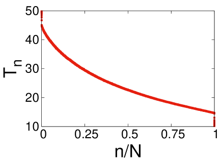
Figure 1: The temperature profile of c-FPU-$\beta$ at $(T_{L},T_{R},l,N)=(50,10,4,2^{15})$. One can see the gaps and the varying gradient.

We also note about the arbitrariness of the defined heat conductivity. One can define energy currents and temperature profiles based on the particle index or on the field coordinate Dhar (2008). This is a property of the lattice systems. This arbitrariness makes following confusing situations under the globally far from equilibrium conditions. The density heterogeneity causes the two different temperature gradients, although the steady state values of the energy currents show the quantitative correspondence ($\langle J_{field}\rangle=\langle J_{particle}\rangle$ for PR-6). Then the values of heat conductivity defined by the ratios are different. This difference remains even though the system is of nearly local equilibrium, because the system satisfies the isobaric (not isodense) conditions under the steady heat conduction. In our PR-6 case, however, we observe the density difference takes a rather small value, roughly 10 percent of initial packing density $d^{-1}$. This is negligible for the discussion of the anomaly. In compressed FPU-$\beta$ case there is no arbitrariness, because one can take the lattice constant as large as one wants Mai et al. (2007). We take the particle type observables, e.g. $J_{n+1,n}:=\frac{p_{n+1}+p_{n}}{2}\left(-\frac{\partial V(x_{n+1,n})}{\partial x_{n+1,n}}\right)$ with energy density $e_{n}:=p_{n}^{2}/(2m)+(V(x_{n+1,n})+V(x_{n,n-1}))/2$, through this paper. One can also define the stress along particle coordinates $\sigma_{n+1,n}=-\frac{\partial V(x_{n+1,n})}{\partial x_{n+1,n}}$. It gives the pressure of the steady state (in the sense of particle coordinates) conforming to the virial theorem.

III Results

III.1 Result of Nonequilibrium Simulation

Now we observe the kinetic temperature, which corresponds to the thermodynamic one under the local equilibrium condition (, $(T_{n+1}-T_{n})/T_{n}\ll 1$ for the finite interparticle distance). Here, the kinetic temperature is defined as

$$T_{n}:=\left\langle\frac{p_{n}^{2}}{m_{n}}\right\rangle.$$ (16)

We use the bracket $\langle\rangle$ to express the long time average.

Figure 1 is the temperature profile of c-FPU-$\beta$ under the steady heat conduction at $(T_{L},T_{R},l,N)=(50,10,4,2^{15})$ and shows the gaps at the edges and the gradient varying at the bulk. As $N$ increases, the gaps are slowly decreasing and the varying gradient remains . The situation of the PR-6 case is the same with it. We consider the points. Firstly, it is necessary to remove the boundary gap, which can show the convergence of pretense Hatano (1999), for the accurate observation of the system size dependence. Secondly, the spatially varying gradient means the spatially varying heat conductivity.

Then we define heat conductivity in two ways to discuss its system size dependence and its spatial variance. $J_{n+1,n}$ is independent of the index in the average of the steady state if the $n,n+1$th particles have no interaction with reservoirs. So we simply call it $J$. Firstly, to study the system size dependence, we introduce the bulk averaged gradient $\overline{\nabla_{n}T_{n}}$, which is given by the linear fitting of $T_{n}$ in $1/4\leq n/N\leq 3/4$, and define the following heat conductivity,

$$\bar{\kappa}(N):=\langle J\rangle/\overline{\nabla T}.$$ (17)

Here we call it bulk heat conductivity. We discuss the anomaly of the bulk through this observable under an assumption that the effect of the discontinuities is negligible. This assumption is valid in nonintegrable large systems. These gaps occur within the reservoir-attached particles at the edges, so they come from purely interfacial resistance. Secondly, to study the spatial variance, we introduce the segmented averaged gradient $\widehat{\nabla_{n}T_{n}}$, which is given by the linear fitting of $T_{n}$ in a sufficiently narrow temperature range sufficiently slowly varying, and define the following heat conductivity with the assumption that $\widehat{\nabla_{n}T_{n}}$ is a function of the average temperature of each segment and $N$,

$$\kappa(T;N):=\langle J\rangle/\widehat{\nabla T}.$$ (18)

Now we call it local heat conductivity. We took two ways to prepare the data of such a temperature range. One is that we equally divide the data 16 (or 32) and cut out $T_{n}$ of the reservoir-attached particles. The other is that we set ($T,\Delta\ll T$) and extract $T_{n}$ satisfying the condition $|T_{n}-T|<\Delta$. Our assumption of local heat conductivity is valid in the systems of normal heat conduction. Heat conductivity of normal heat conduction depends only on the local thermodynamic quantities, although that of anomalous heat conduction depends also on the positions and on the system sizes. Then, this observable lets us know the temperature dependence of the heat conductivity under the isobaric conditions of the pressure $P$ given by the boundary conditions, if the system recovers the intensive property of heat conductivity. We study the asymptotic master curve of the intensive heat conductivity. We can observe such temperature dependence at once under the globally far from equilibrium conditions.

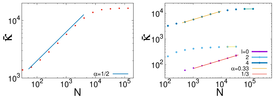
Figure 2: Bulk heat conductivity (Left: PR-6, Right: c-FPU-$\beta$). Parameters are $(T_{L},T_{R},d)=(4,1,3/4)$ for PR-6 and $(T_{L},T_{R},\gamma,l)=(50,30,2,4)$ for c-FPU-$\beta$. They show the convergence except c-FPU-$\beta$ at $l=0$. The transient exponents are $1/2$ in PR-6 and $0.33$ in c-FPU-$\beta$ at $l=4$. For accuracy, we check the power of the last two points in c-FPU-$\beta$ at $l=2,4$ as an indicator of the convergence. The powers are $0.018(l=2)$ and $0.009(l=4)$, which show the quantitative evidence of the convergence.

III.1.1 System size dependence of bulk heat conductivity

Figure 2 is the result of the bulk heat conductivity $\overline{\kappa}$ and shows the convergence in some ways. $\overline{\kappa}$ of PR-6 shows the transient anomalous scaling $\alpha=0.498\pm 0.005$ in $10^{2}\lesssim N\lesssim 10^{4}$ (the exponent of which is fitted in $2^{7}\leq N\leq 2^{12}$ ) and the recovery of normal heat conduction without showing the FH scaling $\alpha=1/3$. $\overline{\kappa}$ of c-FPU-$\beta$ is somewhat strange. It shows the FH anomalous scaling $\alpha=1/3$ at $l=0$, consistent with previous reports Lepri et al. (1997); Mai et al. (2007), but it shows the convergence at $l=2,4$. Particularly, at $l=4$, it shows the anomalous scaling $\alpha=0.330\pm 0.006$ in the transient $N$-dependence (fitted in $2^{9}\leq N\leq 2^{13}$ ), which is almost the FH exponent 1/3. It suggests that the convergence should occur after the FH scaling, in the continuum limit.

$\overline{\kappa}$ of PR-6 shows the divergence with the exponent $\alpha\simeq 1/2$ in $10^{2}\lesssim N\lesssim 10^{4}$ and the convergence at larger sizes. This convergence is consistent with Gendelman and Savin (2014). Its exponent $\alpha\simeq 1/2$ is larger than FH scaling $\alpha=1/3$ and just the second universality exponent van Beijeren (2012); Hurtado and Garrido (2015). The intensive behavior remains even at $N\sim 10^{5}$. As recently reported, diatomic hardcore shows the convergence if their chosen parameters are nearly integrable Chen et al. (2014). Some nearly integrable systems may show significant slow-down to obey the prediction of the continuum theory like in the FPU-problem Spohn (2015). However, our choice of parameters provides the strong nonlinearity, although PR-6 has integrable in some limits (See Settings). We need another explanation of the convergence. It might generate the ballistic transport of the hardcore by the local thermal activation to cause this result. This mechanism is consistent with the dissociation-induced recovery proposed in Gendelman and Savin (2014).

$\overline{\kappa}$ of c-FPU-$\beta$ shows the anomaly at $l=0$ but the converging behavior at $l=2,4$ and we observe the transient anomaly at $l=4$ where the exponent is the FH $\alpha\simeq 1/3$. Firstly, the result at $l=0$ is consistent with the ordinary understanding of anomalous heat conduction Lepri et al. (1997); Mai et al. (2007). The difference of the trend from the previous results at $l=0$ with small sizes is caused by the difference of reservoirs and by the definitions of the temperature gradient. In our case, the number of the attached particles is slightly larger, so the boundary resistance is rather small, and the direct measurement of gradients reduces the effect of temperature gaps to the observable. Secondly, $\overline{\kappa}$ at $l=2$ changes the $N$-dependence completely from the case at $l=0$ and shows the converging behavior throughout the observation. This is inconsistent with ordinary predictions Narayan and Ramaswamy (2002), then we calculated $\overline{\kappa}$ until $N>10^{4}$ but the results were the same. Here we introduce the power measured from the last two points as the indicator of convergence. The power is $\alpha\simeq 0.018$ at $l=2$, almost 20 times smaller than the predicted exponents. The increase goes to be saturated. At the last, $l=4$ is the delicate case. We got the transient exponent $\alpha\simeq 1/3$ in $10^{2}\lesssim N\lesssim 10^{4}$ , which is consistent with the FH theory, but $\overline{\kappa}$ shows another trend at large $N$. There is a plateau at larger sizes. We checked the power from the last two points and got $0.009$. It is the convergence. The weak exponents in FPU-$\alpha\beta$ at some parameters are already observed in Savin and Kosevich (2014), but the converging behavior like our case was not reported in their studies. We can see the transient exponent smaller than 0.1 in $l=2$ case, so it may correspond to their reports of such weak exponents. The difference would be caused by the temperature or by finite size effects. We chose the high temperature ($T\geq 10$), highly nonlinear, and $N>10^{4}$, but their choice was low $T(\leq 0.1)$, weakly nonlinear, and $N<10^{4}$. Actually, the long time tail is sensitive to the energy. The result in Di Cintio et al. (2015) showed the normal-anomalous crossover around $e\sim 0.1$ in FPU-$\alpha\beta$ (at $\alpha=0.1$) of the same unit with us. Repeatedly we note the high-temperature of our system. It is also hard to suppose the possibility of dissociation because of the system property. This is directly checked by the following results of the temperature dependence in the local heat conductivity.

One can doubt whether our results are transient plateaus. The flattening before the FH scaling is actually reported in the previous research Das et al. (2014b). Our case of FPU-$\beta$ also has such a flattening at $l=2,4$ in $N\lesssim 10^{3}$. However, one can see the convergence which is after the FH scaling at $l=4$. This is not included in their studies. next we study the local heat conductivity to avoid the rash conclusion, although our results of bulk heat conductivity suggested the recovery of the intensive property accompanying the increase of pressure.

III.1.2 Temperature dependence of
intensive local heat conductivity

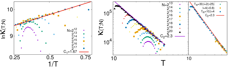
Figure 3: Local heat conductivity (Left: PR-6, Center and Right: c-FPU-$\beta$). Parameters are $(T_{L},T_{R},d)=(4,1,3/4)$ for PR-6 and $(T_{L},T_{R},l)=(50,10,4)$ for c-FPU-$\beta$ in the center panel. The right panel shows the values of FPU-$\beta$ at the largest size of our observations with multiplication of normalization factors. They can be fitted with a unique curve approximately. One can observe the two different types of temperature dependence: the Arrhenius type connected with the thermally activated recovery in PR-6 and the non-Arrhenius type in c-FPU-$\beta$, suggesting another process from thermal activation.

Figure 3 is the result of local heat conductivity $\kappa$ and shows the two asymptotic master curves $\kappa(T;\infty)$ accompanying the recovery of normal heat conduction. Here we call the suggesting master curve $\kappa(T;\infty)$. Although the secured convergence of $\kappa(T;N)\to\kappa(T;\infty)$ in the thermodynamic limit is still controversial, these $N$-independent curves are the strong evidence of the recovery. Apparent $N$-dependence of $\kappa$ means the breakdown of our assumption that the local heat conductivity is described by the local $(T,P)$, and one can see such $N$-dependence only at small sizes. From the master curves, one can see the Arrhenius $T$-dependence in PR-6 which corresponds to the thermal activation of dissociation Gendelman and Savin (2014) and the non-Arrhenius one in c-FPU-$\beta$, which corresponds to a different mechanism from thermal activation.

$\kappa$ of PR-6 shows the recovery of the intensive property and the Arrhenius temperature dependence,

$$\kappa(T,\infty)\sim e^{C_{1}/T}.$$ (19)

The recovery began from the bulk. $C_{1}$ is estimated as $C_{1}\simeq 1.67\pm 0.04$ from our fitting. It is already reported that soft rod systems also show the Arrhenius type heat conductivity given by the GK formula Gendelman and Savin (2014), and they claimed the effective vacancy, dissociation should cause the normal heat conductivity. Such a mechanism would be also realized in this case. The local dissociation is naturally understood as the high energy property in this system (integrable hardcore).

$\kappa(T;N)$ of compressed FPU-$\beta$ at $(l,T_{R})=(4,10)$ recovers the intensive property from the hotter side of the bulk and converges to the power-law curve,

$$\kappa(T;\infty)\sim T^{-C_{2}}.$$ (20)

$C_{2}$ is estimated as $C_{2}\simeq 2.30\pm 0.01$ from our fitting. We note the replacement of $T_{R}$ ($30\to 10$) is done to obtain the sufficiently wide temperature range. The result looks robust against the replacement. Figure 3 (Right) shows the values of FPU-$\beta$ at the largest size of our observations ($(T_{R},l)=(30,2),(30,4),(10,4)$, corresponding size $N=2^{15},2^{17},2^{20}$) with multiplication of normalization factors ($\times 25,0.8,1$ respectively). They can be roughly fitted with a unique curve. The non-Arrhenius $T$-dependence suggests another mechanism from some thermal activation. Taking into consideration the high $T$ property of this system, the result of bulk heat conductivity and this non-Arrhenius $T$-dependence, one can expect that this recovery of the intensive property may be understood with some continuum theory. We also observed the different exponent from already reported $\kappa\sim T^{1/4}$ scaling of zero pressure FPU-$\beta$ Aoki and Kusnezov (2001). The cause may be provided from the convergence of the heat conductivity or the pressure dependence of the heat conductivity because of the effect that the density fields of FPU-$\beta$ becomes spatially non-uniform to satisfy the constraint of uniform $(P,J)$ conditions except $P=0$. We also observed almost the same scaling at $l=2$, then it may come from the normal-anomalous crossover. More accurate discussions on this change of the $T$-dependence across the crossover need other experiments from ours. We firstly took the assumption that the global coupling is negligible. This assumption cannot be applied in anomalous heat conduction. Our interest is the difference of the temperature dependence from the already reported Arrhenius one and it was shown, so we do not go into the detailed discussion of this difference here.

III.2 Result of Equilibrium Simulation

It was suggested through the observations of steady heat conduction that there should be a thermally activated recovery of the heat conduction and that of continuums. Particularly, the latter case showed a striking negative example for ordinary fluctuating hydrodynamic predictions. Then we also study the convergence of heat conductivity through the observations of total energy current power spectra under the isolated equilibrium periodic boundary conditions to check our problematic result. Here we assume the equivalence of ensembles and change the boundary conditions from the isobaric isothermal $\langle\rangle^{eq}_{T,P}$ to the isothermal isodense $\langle\rangle^{eq}_{T,l}$. We studied its power spectra $|\hat{J}(\omega)|^{2}$, the Fourier components of the correlations $\langle\hat{J}(0)\hat{J}(t)\rangle^{eq}_{T,l}$, and their $l$-dependence.

We beforehand discuss the validity of such equivalence. It is necessary to characterize the heat conductivity by a single value of temperature $T$ that the temperature difference is sufficiently small in the correlation length of the energy current, but such a length does not exist in the systems of anomalous heat conduction Pomeau and Resibois (1975); Das et al. (2014a). The quantitative correspondence of the heat conductivity in globally far from equilibrium with the correlation function in the isolated periodic boundary is actually a delicate problem Casati and Prosen (2003); Das et al. (2014b). Nevertheless, one can observe the long time tails of the currents under the isolated periodic boundary conditions and these scalings of the anomaly show the correspondence even with such changes of boundaries (see the $l=0$ case of Figure 4), furthermore, one can see the correspondence well because of the absence of boundary perturbations Lepri et al. (1998); Hatano (1999).

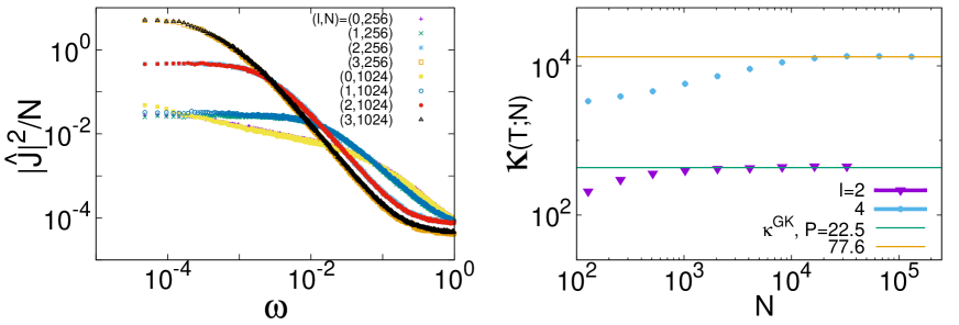
Figure 4: Left: Normalized power spectra of the total energy currents $|\hat{J}(\omega)|^{2}/N$ of c-FPU-$\beta$ at $T=30$ in $10^{-5}\lesssim\omega\lesssim 1$. Right: Comparison between the local heat conductivity at the averaged temperature $\bar{T}$ of steady heat conduction and the corresponding value given by the Green Kubo formula. One can see the anomalous scaling $|\hat{J}(\omega)|/N\sim\omega^{\alpha}$ at small $\omega$ of $l=0$, but Lorentzian$|\hat{J}(\omega)|^{2}/N\sim a/(1+(b\omega)^{2})$ recovers with $l$ increasing ($l=2,3$). There is no system size dependence at $l=2,3$. The trends of (a,b) that (a,b) increase with $l$ are consistent with Figure 2. Pressure looks to suppress the long time tail. The comparison of heat conductivity (Right) shows the consistent convergence of heat conductivity in highly compressed FPU-$\beta$.

Figure 4 (Left) shows normalized power spectra of total energy currents $|\hat{J}(\omega)|^{2}/N$ in compressed FPU-$\beta$ at $T=30$. The anomalous scaling $|\hat{J}(\omega)|^{2}/N\sim\omega^{-\alpha},\alpha=1/3$ is observed in the $l=0$ case of zero pressure. The strong exponent observed at high frequencies corresponds to the next FH exponent $4/3$. However, $l=1$ case shows no FH scaling at low frequencies although one can see the next FH $4/3$ tails at high frequencies. Then it asserts the FH tail in low frequencies is suppressed by the compression. The scaling changes to the Lorentzian at highly compressed cases ($l=2,3$) and one can see the clear suppression of the anomaly at low frequencies. The trend in the Lorentzian of the height and that of the time scale are consistent with our experiment of steady state heat conduction that they increase with compression. We checked the $N$-convergence of the Lorentzian and the results at $N=256,1024$ were the same. In the ordinary understanding, if the ad hoc cutoff of the anomaly $\omega>2\pi c/N$ is valid also under this condition, the spectra at $l=1,2,3$ should show the long time tails at the same area with $l=0$ case, except the improbable explosion of $t_{m}$ with $l$-increasing, because the sound velocity is only doubled through the $l$-increasing ($l=0\to 3$ at $T=30$). The result that there is only the 4/3 exponent (no 1/3) at $l$ = 1 and the Lorentzian recovery at $l=2,3$ suggests that the compression (pressure) should induce the suppression.

This result of equilibrium correlations should show the quantitative correspondence with our result of steady heat conduction if the convergence is not a fake. The Green Kubo formula requires that a variable given by the equilibrium correlations $N^{-1}\int^{\infty}_{0}dt\langle\hat{J}(0)\hat{J}(t)\rangle^{eq}_{T,P}$ and heat conductivity of the system $\kappa_{*}(T,P,N)$ take a same value, that is

$$\lim_{N\to\infty}\left(\frac{1}{N}\int^{\infty}_{0}dt\langle\hat{J}(0)\hat{J}(t)\rangle^{eq}_{T,P}-\kappa_{*}(T,P,N)\right)=0.\hskip 16.0pt$$ (21)

In general, we should include the other orders of the system and in such a case, one can translate $(T,P)$ into the whole intensive variables conjugate with the conserved fields of the system except $N$. We can expect FPU-$\beta$ should not have such additional orders because of the consistency between equilibrium correlations of FPU-$\beta$ and the prediction of fluctuating hydrodynamics for simple fluids Das et al. (2014a). Furthermore, if the system shows the normal heat conduction, the above relation becomes more tractable. Firstly, energy currents in the systems of normal heat conduction have the finite correlation length, so heat conductivity is not modified under the change of boundaries if the change does not vary $(T,P,N)$. It means

$$\frac{1}{N}\int^{\infty}_{0}dt\langle\hat{J}(0)\hat{J}(t)\rangle^{eq}_{T,P}=\frac{1}{N}\int^{\infty}_{0}dt\langle\hat{J}(0)\hat{J}(t)\rangle^{eq}_{T,l_{*}(T,P)}.$$

We defined $l_{*}(T,P)$ as the compression that gives the pressure $P$ under the temperature $T$ (and $N$). Also, in the system of normal heat conduction, heat conductivity is independent of the observational condition if $(T,P)$ take the same values. It is another consequence of the locality guaranteed in the systems of normal heat conduction. Then, from the above relations, the question about the consistency between the variable given by the equilibrium correlations,

$$\kappa^{GK}(T,l,N):=\frac{1}{N}\int^{\infty}_{0}dt\langle\hat{J}(0)\hat{J}(t)\rangle^{eq}_{T,l},$$ (23)

and our local heat conductivity $\kappa(T,N)$ gives us the hint whether the numerical convergence captures the behavior in the thermodynamic limit. For this investigation, it is enough to check the relation,

$$\lim_{N\to\infty}\left(\kappa^{GK}(T,l_{*},N)-\kappa(T,N)\right)=0.$$ (24)

We note the Green Kubo relation holds even at finite sizes if the observational condition and the size are the same, which can be proved with fluctuation theorem Seifert (2012) (see Appendix), but this is not guaranteed in different sizes or with different boundaries. So, this consistency becomes strong evidence of the convergence in the thermodynamic limit, though we cannot access the limit in rigorous sense.

Figure 4 (Right) shows the consistency between $\kappa^{GK}(T,l_{*},N)$ of equilibrium simulations and $\kappa(T,N)$ of steady heat conduction at the averaged temperature of reservoirs $T=\bar{T}(:=(T_{L}+T_{R})/2)$. As subtle but significant notation, $l_{*}$ and $l$ of nonequilibrium simulations of far from equilibrium conditions should not take the same value in general, because local compression of nonequilibrium simulations takes a different value from $l$. Homogeneity of pressure under the simulation is satisfied for the steady condition, so the choice of pressure avoids meaningless confusion. The values of pressure in nonequilibrium simulations are $P\simeq 22.5(l=2),77.6(l=4)$ with Langevin reservoirs ($T_{L}=30,T_{R}=50,\bar{T}=40,\gamma=2,N=2^{15}$, attached particle number 10+10) at the edges. The values of pressure were robust against the size in our case. We measured $\kappa^{GK}$ at the rather small sizes ($N=1024(l=2),256(l=4)$) on receiving the $N$-independence as seen in the left panel of Figure 4. Both cases of different compression $l=2,4$ show the quantitative correspondence with Green Kubo values at large sizes. The transient exponent at $l=4$ is consistent with the corresponding bulk heat conductivity. This system shows the numerical consistency of two variables under the different conditions (of sizes and of boundaries). It strongly asserts the normal heat conduction which remains at the larger sizes.

III.3 Result of Analysis

Our simulations showed two different types of temperature dependence on intensive heat conductivity. They suggest two mechanisms in the recovery of Fourier’s law. The Arrhenius form connects to a thermally activated inhibitor and the non-Arrhenius one suggests a continuum mechanism different from the former. Here, we try to explain these processes phenomenologically.

III.3.1 Transition-state theory of
thermally activated dissociation

Here we estimate the coefficient of the Arrhenius $T$-dependence in PR-6 along the scenario of thermally activated dissociation proposed in Gendelman and Savin (2014). In PR-6, there is no FH scaling before the convergence and the temperature dependence is the Arrhenius form. This result suggests the possibility that some non-continuum effect would suppress the anomaly. According to them, this convergence is caused by the effective vacancy (dissociation) formation. Now we assume it as an effective point defect and estimate the effective activation energy to compare with our numerical result.

If one can define the maximum energy state on each vacancy formation path, according to the transition-state theory, the vacancy formation ratio $P_{*}\sim\exp(-E_{*}/T)$ can be decided by the minimum of their energy cost Eyring (1935), i.e. $E_{*}$ is the energy difference between the maximum energy and the minimum energy on the path to generate a defect with the smallest energy cost. In this case, the path corresponds to the quasi-static path, then $E_{*}$ corresponds to the minimum energy benefit to make a vacancy at the bulk. Concretely, as the minimum work to make a vacancy of the characteristic length $d$ at the bulk including $N$ particles, one can estimate $E_{*}$ as

$$E_{*} \sim N\left(V\left(d\left(1-\frac{1}{N}\right)\right)-V(d)\right)-V(d)$$ (25)

$$\simeq -\frac{\partial V(d)}{\partial d}d-V(d).$$ (26)

Then, the minimum length which has a vacancy in average would be

$$N_{*}\sim P_{*}^{-1}\sim e^{E_{*}/T}.$$ (27)

Then, assuming the scaling $\kappa\sim$ $N^{\alpha}$ is saturated at $N_{*}$, the temperature dependence of $\kappa$ is given by

$$\kappa\sim N_{*}^{\alpha}\sim e^{\alpha E_{*}/T}.$$ (28)

We compare the estimation with the numerical value: $C_{1}\simeq 1.7\sim 2$. We derive the value: $C_{1}\sim 2.341\sim 2$ from the above discussion with $\alpha\simeq 1/2$ of the simulation. The mechanism of the recovery caused by the thermally activated point defect gives an approximate picture to this convergence, even though the dissociation is not well defined in this system. One can take elastically colliding systems like in Gendelman and Savin (2014) as the model systems for more accurate treatments, where the dissociation is safely defined.

III.3.2 Fluctuating hydrodynamic description of
the pressure-induced recovery

We investigate how the pressure fluctuation changes the observed transport coefficients here. Our numerical simulations suggest that there would be a pressure-induced mechanism of the recovery of Fourier’s law in one dimensional momentum-conserving systems. This non-Arrhenius temperature dependence is inconsistent with the scenario of thermally activated dissociation, so we should consider the recovery with some continuum theory. Here we consider the mechanism with the fluctuating hydrodynamics.

One dimensional full fluctuating hydrodynamic equations describe the slow motion of the conserved quantities (: mass, momentum and energy) and consist of the following equations of continuity, writing $(\rho,v,e)$ as mass density, velocity and energy density,

$$\left\{\begin{array}[]{lll}\partial_{t}\rho+\partial_{x}(\rho v)=0\\ \partial_{t}(\rho v)+\partial_{x}(\rho v^{2}+\sigma)=0,\hskip 3.0pt\sigma=P-\mu\partial_{x}v-s\\ \partial_{t}e+\partial_{x}J=0,\hskip 3.0ptJ=ev+v\sigma-\kappa\partial_{x}T-g\hskip 22.0pt.\end{array}\right.$$ (32)

Here $(P,T)$ express pressure and temperature and are the functions of mass density and internal energy density ($\rho,e-\rho v^{2}/2$). ($\mu,\kappa$) are bulk viscosity and heat conductivity. $(s,g)$ are random stress and random heat current. The currents of momentum and those of energy include dissipation terms which consist of the deterministic part expressed as the linear irreversible process and the stochastic part satisfying fluctuation dissipation relation (FDR) Kubo et al. (2012). $(s,g)$ are described by the white noise as a consequence of the central limit theorem, and satisfy the following relations expressing the local FDR, using $\langle\rangle$ as the noise average,

$$\left\{\begin{array}[]{lll}\langle s(x,t)s(x^{\prime},t^{\prime})\rangle&=&2\mu T\delta(x-x^{\prime})\delta(t-t^{\prime})\\ \langle g(x,t)g(x^{\prime},t^{\prime})\rangle&=&2\kappa T^{2}\delta(x-x^{\prime})\delta(t-t^{\prime})\\ \langle s(x,t)g(x^{\prime},t^{\prime})\rangle&=&0.\end{array}\right.$$ (36)

In addition, the high wave number cutoff $\Lambda$ is assumed because of the non-continuum area of short-wavelength.

We want to derive some simple model to study the effect of compressibility based on these equations here. We treat our equilibrium result as the observation of the anomaly suppression, then do not consider the nonequilibrium effects. Our treatment to discuss the convergence also neglects the nonlinear terms of dissipation terms, because they are irrelevant even in the inviscid scaling Spohn (2015). We restrict our attention in such a parameter range. We write $(\rho,u:=\rho v,e)$ as mass density, momentum density and energy density, and study the fluctuations$(\delta\rho,u,\delta e)$ from the base of a static equilibrium state $(\rho_{0},0,e_{0})$. Their motion is described by the following equations, at the lowest order of nonlinearity neglecting irrelevant dissipative nonlinear terms,

$$\left\{\begin{array}[]{lll}\partial_{t}\delta\rho+\partial_{x}u=0\\ \partial_{t}u+\frac{1}{\rho_{0}}\partial_{x}u^{2}\\ =-\left(\frac{\partial P}{\partial\rho}\right)_{0}\partial_{x}\delta\rho-\left(\frac{\partial P}{\partial\rho}\right)_{0}\partial_{x}(\delta e-\frac{u^{2}}{2\rho_{0}})+\nu_{0}\Delta u+\partial_{x}s_{0}\\ \hskip 10.0pt-\frac{1}{2}\partial_{x}\left[\left(\frac{\partial^{2}P}{\partial\rho^{2}}\right)_{0}(\delta\rho^{2})+2\left(\frac{\partial^{2}P}{\partial\rho\partial e}\right)_{0}\delta\rho\delta e+\left(\frac{\partial^{2}P}{\partial e^{2}}\right)_{0}\delta e^{2}\right]\\ \partial_{t}\delta e+\frac{1}{\rho_{0}}\partial_{x}(u\delta e)\\ =-h_{0}\partial_{x}u+\kappa_{0}\left(\frac{\partial T}{\partial\rho}\right)_{0}\Delta\delta\rho+\kappa_{0}\left(\frac{\partial T}{\partial e}\right)_{0}\Delta\delta e+\partial_{x}g_{0}\\ \hskip 10.0pt-\frac{e_{0}}{\rho_{0}}\partial_{x}\left(u\frac{\delta\rho}{\rho_{0}}\right)-\partial_{x}\left[u/\rho_{0}\left(\left(\frac{\partial P}{\partial\rho}\right)_{0}\delta\rho+\left(\frac{\partial P}{\partial\rho}\right)_{0}\delta e\right)\right]\,\,.\end{array}\right.$$ (44)

We defined ($\nu_{0}:=\mu_{0}/\rho_{0},h_{0}:=(P_{0}+e_{0})/\rho_{0}$) and $0$ is the indicator of original equilibrium values. The derivation of the above equations is almost the same with  Spohn (2015). He chose the particle distance as a conserved quantity instead of mass, but this is basically equivalent Spohn (2014). The nonlinear terms arise from pressure nonlinearity and Galilean invariance of fluids. Pressure nonlinearity is well studied in his papers. He assumed fluid equations in the particle currents (Lagrangian description) and no streaming terms appear in the decription. Compared with pressure, streaming terms seem to have attracted less attention in spite of the famous mechanism of the anomaly induced by them Forster et al. (1977). Then we continue the analysis with the approximation of weak pressure fluctuations here to study the other origin of nonlinear effects. For further approximation, we treat the pressure fluctuations as the perturbations and neglect the corresponding nonlinear terms. We also neglect the nonlinear term including ($\delta\rho/\rho_{0}$) taking into account the arbitrarily large lattice constant of lattice sytems, then get the following equations,

$$\left\{\begin{array}[]{lll}\partial_{t}\delta\rho+\partial_{x}u=0\\ \partial_{t}u+\frac{1}{\rho_{0}}\partial_{x}u^{2}=-Y_{0}\partial_{x}\delta\rho-Z_{0}\partial_{x}\delta e+\nu_{0}\Delta u+\partial_{x}s_{0}\\ \partial_{t}\delta e+\frac{1}{\rho_{0}}\partial_{x}u\delta e=-h_{0}\partial_{x}u+D_{0}\Delta\delta e+E_{0}\Delta\delta\rho+\partial_{x}g_{0}\,\,.\end{array}\right.$$ (49)

(50)

Here we defined the coefficients $Y_{0}:=\left(\frac{\partial P}{\partial\rho}\right)_{0}$, $D_{0}:=\kappa_{0}\left(\frac{\partial T}{\partial e}\right)_{0}$, $Z_{0}:=\left(\frac{\partial P}{\partial\rho}\right)_{0}$ and $E_{0}:=\kappa_{0}\left(\frac{\partial T}{\partial\rho}\right)_{0}$. $D_{0}$ is positive in general. $h_{0}$ can take the negative values, e.g. negative $h_{0}$ corresponds to some expanded states in FPU-$\beta$. In $Z_{0}=0$ case, corresponding to zero pressure in FPU-$\beta$, $Y_{0}$ is positive because the sound velocity takes the real value. Particularly, ($Y_{0},Z_{0},h_{0},E_{0}\to 0$) corresponds to the dynamics of the passive scalar on noisy Burgers fluids Drossel and Kardar (2002), and the divergence of observed transport coefficients ($\nu,D$) obeys the inviscid scaling Forster et al. (1977); Kardar et al. (1986). Then, one can see this model as a minimal model to study the effect of compression.

The explicit calculation of renormalization into the observed transport coefficients on these equations clarifies how the pressure fluctuations affect the observed heat conductivity as a consequence of Galilean invariance. In particular, $Z=0$ ($Z$ negligible) case is consistent with decoupling hypothesis in Spohn (2015), where the heat mode is passive to the sound modes, and we choose the parameter. Here, those waves are defined as the plane waves of perfect fluids. The propagation speed is zero in heat mode and the sound speed in sound modes. Original decoupling hypothesis assumes that relation between plane waves only at the long wavelength and means the asymptotic irrelevance of contribution from the heat to the sounds. The prediction based on the approximation is tested with good correspondence Das et al. (2014a), so this hypothesis would capture the truth. We also emphasize $Z=0$ is the unique parameter satisfying decoupling hypothesis except special sets of the coefficients. We put the MCT results under this parameter choice, which renormalizes the contribution of the higher wave length fluctuations at once in the lowest order of nonlinearity  Forster et al. (1977). The result of heat diffusion coefficient takes the following value in the long wavelength and low frequency limit,

$$\frac{D_{R}}{D_{0}} = 1+\frac{T_{0}}{2\pi\rho_{0}\sqrt{Y_{0}}\sqrt{D_{0}(D_{0}+\nu_{0})}}\frac{D_{0}+2\nu_{0}}{D_{0}+\nu_{0}}$$

$$\times\left(2\arctan(W_{0}\Lambda)+\frac{(3D_{0}+\nu_{0})W_{0}\Lambda}{(D_{0}+2\nu_{0})(1+(W_{0}\Lambda)^{2})}\right),$$

$$W_{0} := \sqrt{\frac{D_{0}(D_{0}+\nu_{0})}{Y_{0}}}.$$ (51)

This convergence is consistent with our numerical simulation. We note that the zero sound velocity limit ($Y_{0}\to 0$) recovers the ordinary result of the $D_{R}$ divergence ($D_{R}\to\infty)$. Considering the difference between ours and noisy Burgers solution ($Y_{0}\to 0$ case), one can understand the convergence of the renormalized heat conductivity ($\kappa_{R}\simeq D_{R}/\left(\frac{\partial T}{\partial e}\right)_{0}$) as the cutoff of the anomaly around the characteristic wavenumber $k_{*}:=2\sqrt{Y_{0}}/\nu_{0}$. This wave number is defined as the characteristic wavenumber of the momentum field Green function absorbing the density fluctuations, given by

$$G_{0}(k,t):=\int\frac{d\omega e^{ikt+i\omega t}}{i\omega+\nu_{0}k^{2}-iY_{0}k^{2}/\omega},$$ (52)

to show the effect of compressibility, i.e.

$$G_{0}(k,t)\simeq\left\{\begin{array}[]{ll}e^{-\nu_{0}k^{2}t},&k\gg k_{*}\\ e^{-\frac{\nu_{0}k^{2}}{2}t}\cos(\frac{\nu_{0}k_{*}|k|}{2}t),&k\ll k_{*}.\end{array}\right.$$ (55)

Then the compressibility would be intrinsic for this convergence. As other results, we derived the followings,

$$\frac{\nu_{R}}{\nu_{0}} = \infty,$$ (56)

$$\frac{h_{R}}{h_{0}} = 1+\frac{(D_{0}-E_{0}/h_{0})T_{0}\arctan(W_{0}\Lambda)}{2\pi\nu_{0}\rho_{0}\sqrt{Y_{0}}\sqrt{D_{0}(D_{0}+\nu_{0})}},$$ (57)

and $Y_{R}-Y_{0},Z_{R}-Z_{0},E_{R}-E_{0}=0$. $h_{R}\neq h_{0}$ is understood as the renormalization of the thermal fluctuations into the energy. The value of the renormalized viscosity $\nu_{R}\to\infty$ asserts the result of $D_{R}$ is caused by some breakdown of the hyperscaling because two transport coefficients show the same scaling with sizes if the hyperscaling holds Forster et al. (1977).

However, there are at least three problems for this interpretation. One is the unknown parameter $\nu_{0}$. The above result of $D_{R}$ asserts that the cutoff would be determined by the balance between viscosity and compressibility, but $\nu_{0}$ is not observable. The second one is the correspondence of this result and the previous works which claim the divergence of heat conductivity in the inviscid limit. The third one is $\nu_{R}$ divergence. Some RG flow study can avoid the problems, but the RG study of those equations lacks brevity in spite of the unclear validity of our approximation.

The passive scalar limit, $Z_{0}=h_{0}=E_{0}=0$ extremely simplifies the problem, then we study the RG flow on this condition with believing some universality. This parameter simplification does not change our MCT results for the two transport coefficients $D$ and $\nu$. It means the results of our MCT analysis can be understood based on the following RG discussion. For further simplicity, we do not discuss the slightly messy flow of passive scalar here. Its flow does not affect the flow of the other conserved fields and should show the breakdown of the hyperscaling as the consistency with our MCT analysis (i.e. the value is absorbed into 0 under the flow). Then our starting point is

$$\left\{\begin{array}[]{lll}\partial_{t}\delta\rho+\partial_{x}u&=&0\\ \partial_{t}u+\frac{1}{\rho_{0}}\partial_{x}u^{2}&=&-Y_{0}\partial_{x}\delta\rho+\nu_{0}\Delta u+\partial_{x}s_{0}\end{array}\right..$$ (60)

These equations correspond to fluctuating hydrodynamic equations where pressure is temperature-independent and weakly fluctuates. $c_{0}:=\sqrt{Y_{0}}$ is the original sound velocity. One can do the same diagram calculation with the noisy Burgers case Forster et al. (1977), then we briefly report the results. We introduce the formal nonlinear intensity $\lambda$ and replace $1/\rho_{0}$ with $\lambda_{0}:=1/\rho_{0}$. We write the noise intensity as $\Sigma,\,\Sigma_{0}:=2\rho_{0}\nu_{0}T_{0}$ to avoid the confusion of notation and define the coefficients $\bar{Y}:=4Y/(\nu\Lambda)^{2},\bar{\lambda}:=\lambda\sqrt{\Sigma/(\nu^{3}\Lambda)}$ for preparation.

The renormalization of the contribution from short wavelength $\Lambda>|k|>\Lambda e^{-l},u^{>}:=u\theta(|k|-\Lambda e^{-l})$ to long wavelength $|k|<e^{-l},u^{<}:=u-u^{>}$ and the rescaling along the scaling of $u$, $k^{\prime}:=e^{l}k,\omega^{\prime}:=$ $e^{\int^{l}_{0}z(l^{\prime})dl^{\prime}}$ $\omega,u^{<}=:\zeta u^{\prime}$,$y(l):=\frac{d}{dl}\log\zeta-(z+1/2)$ shape the following RG flow,

$$\frac{d\nu}{dl} = \nu\left(z-2+\frac{\bar{\lambda}^{2}}{2\pi}\right)$$ (61)

$$\frac{d\Sigma}{dl} = \Sigma\left(z-2-2y+\frac{\bar{\lambda}^{2}}{2\pi}\frac{1}{\sqrt{1-\bar{Y}}^{3}}\right)$$ (62)

$$\frac{d\lambda}{dl} = \lambda(-3/2+z+y)$$ (63)

$$\frac{dY}{dl} = Y(-2+2z).$$ (64)

$\zeta$ is chosen to make the same RG flow of $(\nu,\Sigma)$, and $z$ is chosen as $\nu$ fixed at their initial values. The values are

$$y = \frac{\bar{\lambda}^{2}}{4\pi}\left[\frac{1}{\sqrt{1-\bar{Y}}^{3}}-1\right]$$ (65)

$$z = 2-\frac{\bar{\lambda}^{2}}{2\pi}.$$ (66)

Under the choice, the RG flow is reduced to

$$\frac{d\bar{Y}}{dl} = \bar{Y}\left(2-\frac{\bar{\lambda}^{2}}{\pi}\right)$$ (67)

$$\frac{d\bar{\lambda}}{dl} = \bar{\lambda}\left[\frac{1}{2}-\frac{\bar{\lambda}^{2}}{4\pi}\left(3-\frac{1}{\sqrt{1-\bar{Y}}^{3}}\right)\right].$$ (68)

We put the flow in Figure 5. Now one can find four fixed points, trivial Gaussian fixed point $(\bar{\lambda},\bar{\lambda},y,z)=(0,0,0,2)$, the well-known inviscid fixed point $(\bar{\lambda},\bar{Y},y,z)=(\sqrt{\pi},0,0,3/2)$, $\bar{Y}$ divergent Gaussian fixed point $(\bar{\lambda},\bar{Y},y,z)=(0,\infty,0,2)$ and the other non-trivial fixed point $(\bar{\lambda},\bar{Y},y,z)=(\sqrt{2\pi},1-2^{-2/3},1/2,1)$. Here we call it ballistic fixed point because of its $z$ value $z=1$. Gaussian fixed points are unstable in one dimension as already pointed out Forster et al. (1977), and the situation is the same in this analysis. It is noteworthy that only the ballistic fixed point is linearly stable. $\bar{Y}$ divergent Gaussian fixed point is unstable in $\bar{\lambda}>0$, so it would have no meaning because we started the analysis with $\bar{\lambda}_{0}\neq 0$. The inviscid fixed point is unstable to the $\bar{Y}$ direction and stable only in $\bar{Y}=0$. If the system at the point is perturbed to the $\bar{Y}$ direction, $\bar{Y}$ increases and the flow is absorbed to the ballistic fixed point. This result corresponds to the anomaly cutoff in our MCT analysis. We repeat the positivity of $\bar{Y}_{0}$ in this case.

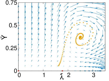
Figure 5: The RG flow field (67),(68) of approximated full fluctuating hydrodynamic equations in the passive scalar limit. There are four fixed points, $(\bar{\lambda},\bar{Y})=(0,0),(0,\infty),(\sqrt{\pi},0),(\sqrt{2\pi},1-2^{-2/3})$. The latter two points are the well-known inviscid fixed point and the non-trivial ballistic fixed point. The linearly stable fixed point is the ballisitc fixed point only. The inviscid fixed point is unstable except in $\bar{Y}=0$. We marked the three fixed points taking finite values and show the typical flow in the same figure. $\bar{Y}$ slowly increases around the inviscid fixed point and the flow is accelerated after the detachment and wraps around the ballistic fixd point.

With the above results, one can interpret the anomaly cutoff of the observed heat conductivity as some crossover between those two fixed points. The cutoff is determined by the characteristic wavenumber $\Lambda_{*}$ where viscosity and compressibility are balanced. $\Lambda_{*}$ is defined as the minimum wavenumber satisfying the following relation,

$$\frac{2c}{\nu(\Lambda_{*})\Lambda_{*}}=1.$$ (69)

These quantities are observable. If the system obeys the inviscid scaling, one can roughly estimate $\nu$ as $\nu(k)\sim k^{-1/3}$ then the viscous fluids have such $\Lambda_{*}$ because of $c>0$. The corresponding system size $N_{*}:=2\pi/\Lambda_{*}$ is also given if $\Lambda_{*}$ exists. Now, the scenario asserted from the results is as follows. At first, heat conductivity increases obeying the inviscid scaling in the small system sizes $N\ll N_{*}$, but the trend changes at $N\sim N_{*}$ and the heat conductivity shows the convergence at the larger system sizes $N\gg N_{*}$, i.e.

$$\kappa\sim\left[\min[N,N_{*}]\right]^{1/3}.$$ (70)

The flow stagnates around the inviscid fixed point, then there can be a certain period to show the anomaly. The result is consistent with the result of c-FPU-$\beta$ at ($l=4,T\gg 1$) where bulk heat conductivity increases with $\alpha\sim 1/3$ transiently and shows the tendency of saturation at larger system sizes. The result at $l=2$ showing the rapid saturation can be interpreted as the case where initial $(\bar{\lambda},\bar{Y})$ are near the ballistic fixed point.

The above scenario would be appropriately modified to include the apparent counter example, the inviscid fixed point $(\bar{Y},\lambda)=(0,\sqrt{\pi})$ in our analysis. This parameter $\bar{Y}=0$ corresponds to the $l=0$ case showing the agreement to the ordinary theories Narayan and Ramaswamy (2002); Spohn (2015). The stability of two nontrivial fixed points would be also changed by the effect of pressure nonlinearity. Even though, we expect full analysis would keep the main ideas of this discussion that the convergence our simulation captured would be connected to the crossover between two fixed points in the intermediate wavelength. According to our RG analysis, there can be a transition in the long wavelength limit of full fluctuating hydrodynamics.

IV Discussions

Here we discuss the correspondence between our results and previous works, the RG flow results (explicit calculations of noisy incompressible fluids, those of noisy Burgers fluids Forster et al. (1977) and the scaling analysis Narayan and Ramaswamy (2002)), MCT results of Full FH (for the scaling of equilibrium correlators Spohn (2015) and for steadily sheared systems Lutsko and Dufty (2002)), numerical simulations and the carbon-nanotube experiments Chang et al. (2008).

Thermally activated dissociation and pressure fluctuations would cause the recovery of Fourier’s law in one dimensional momentum-conserving systems. The integrable systems at the dilute (high-energy) limit (e.g. PR-$\delta$ Savin and Kosevich (2014) and soft rod Gendelman and Savin (2014)) would be the models of the thermally activated recovery. The poly(quasi)-stable interaction potential systems like coupled rotator model would be also in this class by the same reason. The direct calculation of heat conductivity in coupled rotator model with onsite potential predicts the Arrhenius $T$-dependence Pereira and Falcao (2006). With the same mechanism, carbon-nanotube may also show the saturation caused by thermally generated defects which is not avoidable in the real experiments Kittel (2005). The dissociation discussed here is not static and did not get the sufficient test, and the realtion between dissociation class and nearly integrable systems which show the convergence (e.g. diatomic hardcore with small mass difference Chen et al. (2014)) is still unclear. Further study is needed. Also, we note one can see the long time tails of energy currents in diatomic PR-$6$ at the golden mass ratio. The reason would be the nonintegrability in its dilute limit (diatomic hardcore). At the same time, the sum of momentum in each same-mass particles shows the long time tail, which means this observable is effectively conserved. The diatomic systems may need careful treatments Chen et al. (2014); Hurtado and Garrido (2015). The previous numerical simulation reporting the importance of the ballistic behavior in normal heat conduction Li et al. (2015) was criticized because of their zero-temperature simulations Kosevich and Savin (2015), but our following ballistic scaling observation is at the high temperature, where the system shows the anomaly at zero pressure. Potential asymmetry makes non-zero pressure, then this ballistic-inviscid crossover on the RG flow may give some insight to the controvertial systems of the convergence like FPU-$\alpha,\beta$ and LJ Lepri et al. (2015); Chen et al. (2012); Wang et al. (2013); Savin and Kosevich (2014); Das et al. (2014b); Lepri et al. (2005). For the real experiments, if our discussions are right, the dominance of these two effects is not clear, then to find the system showing the two mechanisms (corresponding to two temperature dependence) is also of interest. The multi-particle collision system Di Cintio et al. (2015) is intriguing. The recovery of Fourier’s law in the thermodynamic limit should also still be discussed.

The continuum suppression of the anomaly is caused by the response to the pressure fluctuations in our analysis, and then compressibility can be an intrinsic factor. Our analysis considers the pressure fluctuations as the base of the linearized hydrodynamics and the wave number of saturation is decided with the sound velocity ($\sqrt{Y_{0}}$). In incompressible fluids, the pressure effect is the first order of nonlinearity (then $\mathcal{O}(l)$) and the response to the pressure becomes the second order (then $\mathcal{O}(l^{2})$), so the (first derivative) RG flow of incompressible fluids Forster et al. (1977) does not include this saturation. In zero sound velocity limit, our result corresponds to the noisy Burgers result Forster et al. (1977); Kardar et al. (1986). We repeat our RG result demonstrated the instability of the inviscid fixed point to the assignment of compressibility. The property and the validity of our equations in $d>2$-dimensional cases, where the RG flow of Noisy Burgers has an unstable fixed point Forster et al. (1977), should be tested. It may be constructive to derive the ballistic fixed point along the discussion deciding the anomalous exponent Narayan and Ramaswamy (2002) here. Firstly, we rescale time and space as $x=x^{\prime}e^{l},t=t^{\prime}e^{zl}$ and assume the conserved fields we choose $(\rho,{\bf u},e)$ take the same scaling $(\rho,{\bf u},e)=\zeta(\rho^{\prime},{\bf u}^{\prime},e^{\prime})$. Then, if mass conservation law $\partial_{t}\rho+{\bf\nabla u}=0$ is required to be invariant under the RG flow, $t$ and $x$ scale in the same way because of the required assumption. This is the desired exponent $z=1$. This scaling discussion is in contrast to the discussion in Narayan and Ramaswamy (2002) which required the same rescaling of the set $(\rho,{\bf v},e)$, where the scaling ($z=3/2,d=1$) is derived from the requirement of the same scaling of $(\rho,{\bf v},e)$, relevance of nonlinearity in the flow and the scaling invariance of the equal-time equilibrium fluctuations $\int dx^{d}(\rho^{2},{\bf v}^{2},e^{2})$ under the flow (long range Gaussian property in their terms). In their discussions, the scaling dimension of the three variables is $-d/2$ and it corresponds to $-(d/2+z)$ if the variables are treated as densities of the time directions (as a roughly sketched example:$\rho\to\rho\Delta t$) as described in Forster et al. (1977). The second assumption is satisfied in $d<2$ dimension. The last assumption can be understood as the extensive property of the fluctuations. Then, in other words, one can get the ballistic fixed point if one replaces the extensive fluctuations of $(\rho,{\bf v},e)$ with those of $(\rho,{\bf u},e)$ in their discussion. We also note that the scaling exponent $z=1$ is independent of the dimension in this discussion. We do not know the meaning. Our scaling discussion expanded here is of heuristics and apparently has no use for the stability, but our example of the RG flow showed the possibility that compressibility should make the flow around the inviscid fixed point unstable.

In addition, the MCT analysis under sheared conditions (nonequilibrium steady states) already reported the tail strengthening, corresponding to the normal transport Lutsko and Dufty (2002). This may work as an analogy of the possibility that the nonequilibrium effect causes the convergence. They reported that the tail exponent changed at the characteristic wave number of the shear and that the strengthened exponent of the long wave length corresponded to the normal transport. We did not discuss such possibility here, but it is not hard to suppose that the nonequilibrium condition (isobaric but varying temperature) may affect the heat conduction because of the global coupling as in the GK formula Casati and Prosen (2003).

At the last, we go back to the most detailed MCT analysis of equilibrium correlations in one dimensional full FH Spohn (2015) for the discussion of the correspondence. We mention the difference that our analysis and his analysis are based on different equations. He started the analysis from the equations of continuity of conserved quantities (volume, momentum and total energy), study the effect of pressure nonlinearity with MCT and with some approximations, and get the scalings of the autocorrelation functions for the three plane waves of the linearized perfect fluids (one heat mode and two sound modes). Their analysis is based on the linearized hydrodynamics added pressure nonlinearity in. In his analysis, the anomaly is directly connected with the heat-heat mode correlator which becomes to the symmetric Levy distribution in sound cones propagating at the sound speed. His prediction is already tested in some anomalous systems with good agreements, but some deviation was also reported Das et al. (2014a). He used some approximations, however, he also claimed the possibility that his result remains without his approximations in his equations. His claim looks based on the mirror symmetry of sound cones and nonlinear terms of currents. Then the difference with us may come from the starting point equations. Their equations do not include no streaming terms because of the derivative along the constituent particles Spohn (2014), then the nonlinear currents are mirror-symmetric because the pressure depends only on mass and on internal energy. However, our equations include streaming terms and the nonlinear current ($u\delta e$) is mirror-antisymmetric. Our result may assert the significance of this difference. One can have some questions to the validity of our $D_{R}$ convergence, so to get the credit, we also note the result of $D_{R}$ (51) is also the exact solution of the passive scalar diffusion coefficient in the fluids neglecting their temperature dependence of pressure. As another derivation, one can easily get the same diagram of (50) with the same procedure of Bedeaux and Mazur (1974). Then our result has the universality based on the ballistic fixed point in some extent.

To clarify the difference, the test of current fluctuations would be sufficient. His concrete prediction is as follows. Firstly, he decomposed the conserved quantities ${\bf Q}_{n}=^{T}(\Delta x_{n}:=x_{n}-x_{n-1},p_{n},\tilde{e}_{n}:=V(\Delta x_{n})+p_{n}^{2}/(2m))$ into the three plane waves of the linearized perfect fluids $\tilde{\bf Q}_{n}$. If one obtains the linearized equations of perfect fluids $(\partial_{t}+\partial_{x}A){\bf Q}=0$ and the covariance matrix $C\,s.t.\,C_{mn}:=\langle Q_{m}(x,t):Q_{n}(y,s)\rangle^{eq}_{T,P}/(\delta(x-y)\delta(t-s))$, one can define the linear transformation matrix $R$ satisfying the conditions $RAR^{-1}=diag(-c,0,c),RCR^{T}=diag(1,1,1)$ and derive $\tilde{\bf Q}:=R{\bf Q}$. We used $\langle:\rangle^{eq}_{T,P}$ as $\langle f:g\rangle^{eq}_{T,P}:=\langle fg\rangle^{eq}_{T,P}-\langle f\rangle^{eq}_{T,P}\langle g\rangle^{eq}_{T,P}$. One can decide $R$ uniquely except the trivial arbitrariness $\pm 1$. One of the sets takes the following matrix. See Spohn (2014) for details. Here we abbreviate the time and the position for discussing the correlations of equal time and equal place. Shortening $\langle\rangle^{eq}_{T,P}$ to $\langle\rangle$, $\Delta x_{n}$ to $x$ and $V(\Delta x_{n})$ to $V$, and defining

$$\tilde{\Gamma}^{-1} := T^{-1}\left(\langle x:x\rangle\langle V:V\rangle-\langle x:V\rangle^{2}\right)$$ (71)

$$+\frac{T}{2}\langle x:x\rangle$$

and

$$\left\{\begin{array}[]{lll}c&:=&\tilde{\Gamma}\left(\langle(V+Px):(V+Px)\rangle+\frac{T^{2}}{2}\right)\\ \tilde{Z}_{1}&:=&\sqrt{2T}c\\ \tilde{\kappa}&:=&\sqrt{2T\tilde{\Gamma}}\\ \partial_{l}P&:=&-\tilde{\Gamma}\left(\langle V:(V+Px)\rangle+\frac{T^{2}}{2}\right)\\ \partial_{e}P&:=&\tilde{\Gamma}\langle x:(V+Px)\rangle\hskip 3.0pt,\end{array}\right.$$ (77)

we can define $R$ as

$$R := \tilde{Z}_{1}^{-1}\begin{pmatrix}\partial_{l}P&-c&\partial_{e}P\\ \tilde{\kappa}P&0&\tilde{\kappa}\\ \partial_{l}P&c&\partial_{e}P\end{pmatrix}.$$ (78)

These values are easily calculated with the numerical integration of the corresponding canonical values. And then he derived the analytic formulae of $\tilde{\bf Q}$ autocorrelators. One of the heat mode becomes symmetric Levy, and ones of the sound modes become the sound speed propagating KPZ.

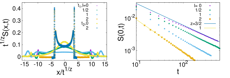
Figure 6: Left: The equilibrium autocorrelation of the heat mode in c-FPU-$\beta$ at $T=1,t=t_{n}\sim 400n/c,N=2048$. Right: $S(0,t)$ in $t\leq t_{2}$. z values of the left panel are chosen as $z=3/2$ at $l\neq 2$ and $z=1$ at $l=2$. One can see the symmetric Levy in sound cones at $l=0$ and the growing bumps around the cones at $l\neq 0$. $S(x,t)$ shows the ballistic scaling at $l=2$. The width scaling is the inviscid one $x/t^{2/3}$ at $l=0$ and the ballistic one $x/t$ at $l=2$. $S(0,t)$ shows the clear crossover.

Here we report the deviation with $l$-increasing in c-FPU-$\beta$, which looks the asymptotic form with respect to $t$-increasing. We set the data of the heat-heat correlator ($\Delta t=0.005,T=1$) in Figure 6. We abbreviate hear-mode autocorrelator $S_{h}$ as $S$ here. We only note about the sound modes that inclined sound-sound correlators already reported in Spohn (2015) is also observed. The symmetric Levy distribution of the heat-heat correlator in the sound cones $S(x,t)\simeq t^{-2/3}f_{I}(x/t^{2/3})$ are observed at $l=0$ Das et al. (2014a), however, the phase difference of the sound cones looks tripled at $l=0.5$. The deviation is consistent with our other results and also with the previous reports Das et al. (2014a). The height scaling looks to change at the same time. The observations of $S(0,t)$ show the change of the height scaling from $z=3/2$ to $z=1$. Furthermore, the heat-mode autocorrelator grows up around cones with the decreasing center top at $l=1,2$. The top is almost negligible at $l=2$. We also note the bumps around the cones are scaled by $x/t$, which is just the ballistic scaling $z=1$. This exponent change and growing bumps mean the scaling crossover from the inviscid scaling $S(x,t)\simeq t^{-2/3}f_{I}(x/t^{2/3})$ to the ballistic scaling $S(x,t)\simeq t^{-1}f_{B}(x/t)$. The sound-heat correlations or the correlation overlaps Das et al. (2014a) may affect the result. If the anomaly remains in his equations, this difference may come from streaming terms. We could not observe the cutoff of the scaling to provide the convergence, although the crossover is observed. It is difficult to observe the anomaly cutoff like $S(x,t)\simeq e^{-t/\tau}t^{-1}f_{B}(x/t)$ at the long time scale as already pointed out in Das and Dhar (2014) and we do not know how the possible cutoff looks to be. We may need the extensive tests of his conjecture.

V Conclusion

Our numerical experiments of steady heat conduction suggested some possible origins of normal heat conduction in one dimensional momentum-conserving systems. The recovery had been explained by the thermally activated dissociation. However, compressed FPU-$\beta$ under the strong compression and of high energy ($l=2,4,T\gg 1$) showed the recovery of Fourier’s law with the non-Arrhenius $T$-dependence of heat conductivity. It suggested the existence of the class of normal heat conduction the origin of which is explained by some macroscopic continuum theory in one dimensional momentum-conserving systems. There would be at least two mechanisms of normal heat conduction. The vanishing long time tails of total energy currents suggested some relation between the novel non-Arrhenius type recovery and the pressure. Then we tried to explain the two mechanisms with corresponding phenomenologies. Firstly, for the case of the Arrhenius $T$-dependence, we studied the coefficient with the transition-state theory following the scenario reported in Gendelman and Savin (2014) that the convergence is caused by the thermal activation of dissociation and got quantitative agreement with our numerical simulations of PR-$6$ in a certain extent. Secondly, for the case of the non-Arrhenius $T$-dependence, we executed the MCT analysis based on full FH equations of a specific limit and got the suggestion that the pressure fluctuations suppressed the anomaly. This was consistent with our numerical result of compressed FPU-$\beta$. The RG flow of further approximated equations asserted the connection between this result and the ballistic fixed point, another nontrivial fixed point from the inviscid fixed point. The fixed point was induced by the compressibility in our RG analysis. Discussing the correspondence with the previous accurate theory of equilibrium correlators Spohn (2015), we found the possibility of the inviscid-ballistic crossover of the heat mode autocorrelator. Further investigation is needed to examine the possibility of normal heat conduction in one dimensional momentum-conserving systems.

Appendix A Derivation of the Green Kubo formula

We derive the Green Kubo formula of the normal heat conduction here in two ways. One of them (102) is the expansion from the globally equilibrium conditions and the other (115) is the expansion from the locally equilibrium conditions. In the far from equilibrium conditions, one cannot use the former, but can use the latter.

A.1 Setting

Let us consider a system that connects to two stochastic reservoirs at the edges. Each reservoir has its connecting area and satisfies the local detailed balance condition. We assume the time-reversal symmetry of the system Hamiltonian and the nearest-neighbor interaction (“short range” interaction). We further assume the unique steady state ensemble $P^{st}$ independent of the initial conditions. Here we consider the macroscopic variables along the particle index, but can translate it to that along the field coordinate $(A_{i}\to A(x)=\sum_{i}A_{i}\delta(x-x_{i}))$. Under that translation, the choice of the variable $r_{i}(:=x_{i+1}-x_{i})$ in the expansion from the locally equilibriums would be translated into that of the mass density $\rho(x)=\sum_{i}m_{i}\delta(x-x_{i})$. Also, one can extend this discussion to the case having additional order parameters.

We describe the fundamental relation to deive the formula as the preparation. We note $\Gamma$ as the phase space coordinate and $\mathcal{H}$ as the system Hamiltonian. $h_{i}$ is the $i$-th particle energy density, $j_{i+1,i}$ is the corresponding energy current and $r_{i}$ is the $i$-th particle compression here. $\beta_{\pm}(\beta_{+}>\beta_{-})$ is the temperature of the reservoir $\pm$. Energy conservation law can be written as

$$\partial_{t}h_{i}+j_{i+1,i}-j_{i,i-1} = \sum_{\pm}\dot{Q}^{\pm}_{i}\chi[i\in D_{\pm}],$$ (79)

$$\chi[\mbox{A}] = \left\{\begin{array}[]{ll}1&\mbox{A:true}\\ 0&\mbox{A:false}\end{array}.\right.$$ (82)

$D_{\pm}$ is the connecting area of the reservoir $\pm$ ($|D_{\pm}|\ll N,\,N$:system size) and $\dot{Q}^{\pm}_{i}$ is the energy came from the reservoir $\pm$ to the $i$-th particle per time. By the local detailed balance condition, the path probability on the path $\hat{\Gamma}$ within the time $t\in[0,\tau]$ and that on the time-reversal path $\hat{\Gamma}^{\dagger}$ satisfy the relation,

$$\frac{P(\hat{\Gamma}|\Gamma_{0})}{P(\hat{\Gamma}^{\dagger}|\Gamma_{\tau}^{*})}=e^{-\beta_{\pm}Q_{\tau}^{\pm}}.$$ (83)

Here, $Q_{\tau}^{\pm}$ is defined as $Q_{\tau}^{\pm}:=\int^{\tau}_{0}\sum_{i\in D_{\pm}}\dot{Q}^{\pm}_{i}$, $\Gamma_{0}$ is the initial state of $\hat{\Gamma}$ and $\Gamma_{\tau}$ is the end state of $\hat{\Gamma}$. $*$ is the index that expresses the time-reversal quantity $B^{*}$ of the instantaneous variable $B(\Gamma)$. $P(\hat{\Gamma}|\Gamma)$ is the conditional probability of the path under this thermostat condition.

It is convenient for later discussions to introduce McLennan ensembles (95) Maes and Netočnỳ (2010); Itami and Sasa (2015). Firstly, we note that fluctuation theorem (88) holds for path-dependent variables $\mathcal{A}(\hat{\Gamma})$ because of the existence of the local detailed balance(83). Now we use $\langle\rangle$ as the average of the stochastic reservoir forces. Defining

$$\Sigma(\hat{\Gamma}):=\beta_{\pm}Q_{\tau}^{\pm}+\log\frac{P^{ref}(\Gamma_{0})}{P^{ref}(\Gamma_{\tau}^{*})}$$ (84)

and using ${\dagger}$ as the indicator of the time-reversals of the path-dependent variables ($\mathcal{A}^{\dagger}(\hat{\Gamma})=\mathcal{A}(\hat{\Gamma}^{\dagger})$), one can get

$$\langle\mathcal{A}(\hat{\Gamma})\rangle := \int d\hat{\Gamma}P(\hat{\Gamma}|\Gamma_{0})P^{ref}(\Gamma_{0})\mathcal{A}(\hat{\Gamma})$$ (86)

$$= \int d\hat{\Gamma}^{\dagger}P(\hat{\Gamma}^{\dagger}|\Gamma_{\tau}^{*})P^{ref}(\Gamma_{\tau}^{*})\mathcal{A}(\hat{\Gamma})$$

$$\hskip 10.0pt\times\exp\left(\beta_{\pm}Q_{\tau}^{\pm}+\log\frac{P^{ref}(\Gamma_{0})}{P^{ref}(\Gamma_{\tau}^{*})}\right)$$

$$= \int d\hat{\Gamma}P(\hat{\Gamma}|\Gamma_{0})P^{ref}(\Gamma_{0})e^{\Sigma^{\dagger}(\hat{\Gamma})}\mathcal{A}^{\dagger}(\hat{\Gamma}).$$ (87)

That is

$$\langle\mathcal{A}\rangle=\langle\mathcal{A}^{\dagger}e^{\Sigma^{\dagger}}\rangle.$$ (88)

Secondly, we consider the time evolution of an ensemble $P_{\tau}$ that started from a reference ensemble $P^{ref}$. We choose $\mathcal{A}=\delta(\Gamma^{\prime}-\Gamma_{\tau})$ in the above fluctuation theorem, and get

$$P_{\tau}(\Gamma^{\prime}) = \langle\delta(\Gamma^{\prime}-\Gamma_{\tau})\rangle=\langle\delta(\Gamma^{\prime}-\Gamma_{0}^{*})e^{\Sigma^{\dagger}}\rangle$$ (90)

$$= P^{ref}((\Gamma^{\prime})^{*})$$

$$\times\int d\hat{\Gamma}P(\hat{\Gamma}|\Gamma_{0})e^{\Sigma^{\dagger}(\hat{\Gamma})}\delta(\Gamma_{0}-(\Gamma^{\prime})^{*}).$$

We take the limit $\tau\to\infty$, and the steady distribution is expressed as

$$P^{st}(\Gamma) = P^{ref}(\Gamma^{*})$$ (91)

$$\times\lim_{\tau\to\infty}\int d\hat{\Gamma}P(\hat{\Gamma}|\Gamma_{0})e^{\Sigma^{\dagger}(\hat{\Gamma})}\delta(\Gamma_{0}-\Gamma^{*}).\hskip 15.0pt$$

We promise that $\langle\rangle^{st}$ expresses the steady state average. This expression is transformed into another form for the instantaneous variables $B(\Gamma)$. Using the relation $d\Gamma=d\Gamma^{*}$, one can get the tractable form

$$\langle B\rangle^{st} = \int d\Gamma^{*}B^{*}(\Gamma^{*})(P^{st})^{*}(\Gamma^{*})$$ (92)

$$= \int d\Gamma B^{*}(\Gamma)(P^{st})^{*}(\Gamma)$$ (93)

$$= \lim_{\tau\to\infty}\int d\hat{\Gamma}B^{*}(\Gamma)P^{ref}(\Gamma)P(\hat{\Gamma}|\Gamma)e^{\Sigma^{\dagger}(\hat{\Gamma})}.\hskip 8.0pt$$ (94)

Namely,

$$\langle B\rangle^{st} = \lim_{\tau\to\infty}\langle B^{*}e^{\Sigma^{\dagger}}\rangle^{ref}.$$ (95)

We expressed the reference ensemble average as $\langle\rangle^{ref}$.

A.2 Derivation

A.2.1 Derivation-1.
Expansions from globally equilibrium conditions

We consider the expansion from the static globally equilibrium state

$$(\langle r_{i}\rangle^{st},\langle p_{i}\rangle^{st},\langle h_{i}\rangle^{st})=(l,0,e).$$ (96)

Corresponding intensive variables are

$$(\beta P,\beta V,\beta)=(\bar{\beta}P_{0},0,\beta),\,\,\bar{\beta}=\frac{\beta_{+}+\beta_{-}}{2}.$$ (97)

$P$ is pressure and $V$ is averaged velocity. Now we choose

$$P^{ref}=P^{can}_{\bar{\beta}}:=e^{-\bar{\beta}\mathcal{H}}/Z$$ (98)

as the reference ensemble. It means the choice of $(T,l)$. We use $\langle\rangle^{can}_{\bar{\beta}}$ to express the average by the ensemble $P^{can}_{\bar{\beta}}$. Entropy production $\Sigma$ takes the form

$$\Sigma = -\beta_{\pm}Q^{\pm}_{\tau}+\bar{\beta}(\mathcal{H}(\Gamma^{*}_{\tau})-\mathcal{H}(\Gamma))=\Delta\beta Q.$$ (99)

We used the time-reversal symmetry of the Hamiltonian $\mathcal{H}(\Gamma^{*}_{\tau})=\mathcal{H}(\Gamma_{\tau})$ and defined $\Delta\beta:=\beta_{+}-\beta_{-},Q:=(Q_{-}-Q_{+})/2$. Corresponding time-reversals are $\Sigma^{\dagger}=-\Delta\beta Q,\dot{Q}^{*}=-\dot{Q}$. The energy conservation law of the systems at the steady states requires $\sum_{\pm}\langle\dot{Q}^{\pm}\rangle^{st}=0$. Also, the energy balance at the bulk ($n\bar{\in}D_{\pm}$) yields the relation,

$$|\langle J\rangle^{st}| := |\langle j_{n+1,n}\rangle^{st}|=\langle\dot{Q}\rangle^{st}$$ (100)

$$= \lim_{\tau\to\infty}\langle-\dot{Q}e^{-\Delta\beta Q}\rangle^{can}_{\bar{\beta}}$$ (101)

$$= \Delta\beta\int^{\infty}_{0}dt\langle\dot{Q}(0)\dot{Q}(t)\rangle^{can}_{\bar{\beta}}+\mathcal{O}((\Delta\beta)^{2}).\hskip 12.0pt$$ (102)

The sign of $J$ is minus if the reservoir $+$ is at the left and plus if it is at the right. The error from the relation can be large if $\Delta\beta$ is comparable with $\bar{\beta}$ and not negligible in that case.

A.2.2 Derivation-2.
Expansions from locally equilibrium conditions

One can know the steady state value of the energy and the compression through the careful observation even if their values spatially change, and we consider the expansion from the static locally equilibrium conditions

$$(\langle r_{i}\rangle^{st},\langle p_{i}\rangle^{st},\langle h_{i}\rangle^{st})=(l_{i},0,e_{i}).$$ (103)

Spatial homogeneity of pressure is needed to keep the zero value of the momenta, then corresponding intensive variables are

$$((\beta P)_{i},(\beta V)_{i},\beta_{i})=(\beta_{i}P,0,\beta_{i}).$$ (104)

Now we suppose $l_{i}$ and $e_{i}$ are slowly varying quantities in space scaled with the correlation length of microscopic variables (particularly $j_{i+1,i},v_{i}:=p_{i}/m_{i}$). Also, we suppose the temperature gaps at the edges are negligible. If the system shows the normal heat conduction, one can realize them with sufficiently large (but finite) system sizes $N$. Under the condition, one can expand the contribution from the entropy production $\Sigma$ around the local equilibriums. So we take the isobaric local equilibrium ensemble as the reference ensemble,

$$P^{ref}=P^{lc}_{\{\beta_{i}\}_{i},P}:=e^{-\beta_{i}h_{i}-\frac{\beta_{i+1}+\beta_{i}}{2}Pr_{i}}/Z.$$ (105)

It means the choice of $(\{T_{i}\}_{i},P)$. $\beta_{i}$ is chosen as the parameter satisfying the relation,

$$i\bar{\in}D_{\pm},\langle h_{i}\rangle^{lc}_{\{\beta_{i}\}_{i},P}=\langle h_{i}\rangle^{st};\,\,i\in D_{\pm},\beta_{i}=\beta_{\pm}.$$ (106)

We use $\langle\rangle^{lc}_{(\{\beta_{i}\}_{i},P)}$ to express the average by the ensemble $P^{lc}_{\{\beta_{i}\}_{i},P}$. Entropy production takes the value

$$\Sigma = -\beta_{\pm}Q^{\pm}_{\tau}+\beta_{i}(h_{i}(\Gamma^{*}_{\tau})-h_{i}(\Gamma))$$ (108)

$$\hskip 38.0pt+\frac{\beta_{i+1}+\beta_{i}}{2}P(r_{i}(\Gamma^{*}_{\tau})-r_{i}(\Gamma))$$

$$= -\int^{\tau}_{0}dt\left[\beta_{i}(j_{i+1,i}-j_{i,i-1})\right.$$

$$\hskip 38.0pt\left.-\frac{\beta_{i+1}+\beta_{i}}{2}P(v_{i+1}-v_{i})\right]$$

$$= \int^{\tau}_{0}dt\left[(\beta_{i+1}-\beta_{i})j_{i+1,i}-\frac{\beta_{i+1}-\beta_{i-1}}{2}Pv_{i}\right].\hskip 18.0pt$$ (109)

The time-reversals are $\Sigma^{\dagger}=-\Sigma,j^{*}_{i+1,i}=-j_{i+1,i}$. Then the averaged value of the current at the bulk $n\sim N/2$ can be estimated as

$$\langle J\rangle^{st}:=\langle j_{n+1,n}\rangle^{st}$$ (112)

$$= \lim_{\tau\to\infty}\left\langle-j_{n+1,n}\right.$$

$$\hskip 20.0pt\left.\times e^{-\int^{\tau}_{0}dt[(\beta_{i+1}-\beta_{i})j_{i+1,i}-\frac{\beta_{i+1}-\beta_{i-1}}{2}Pv_{i}]}\right\rangle^{lc}_{(\{\beta_{i}\}_{i},P)}$$

$$= \left\langle j_{n+1,n}(0)\int^{\infty}_{0}dt\left[(\beta_{i+1}-\beta_{i})j_{i+1,i}\right.\right.$$

$$\hskip 10.0pt\left.\left.-\frac{\beta_{i+1}-\beta_{i-1}}{2}Pv_{i}\right]\right\rangle^{lc}_{(\{\beta_{i}\}_{i},P)}+\mathcal{O}((d\partial_{n}\beta)^{2}).$$

$d$ is the largest correlation length of the currents. $\langle j_{n+1,n}\rangle^{lc}_{(\{\beta_{i}\}_{i},P)}=\langle j^{*}_{n+1,n}\rangle^{lc}_{(\{\beta_{i}\}_{i},P)}=0$ follows the time reversal symmetry of the chosen ensemble reflecting $\mathcal{H}^{*}=\mathcal{H}$. This relation corresponds to that derived by Casati & Prosen Casati and Prosen (2003) under the chaotic pictures. However, the estimated error under the anomalous heat conduction is different from the above. Under the condition, the estimated error was $\mathcal{O}((N\partial_{n}\beta)^{2})=\mathcal{O}((\Delta\beta)^{2})$ because there were no scale separations anymore and the correlation length grows to the system size ($d\sim N$). The situation of the system of normal heat conduction is in sharp contrast to it. In the systems of normal heat conduction, this modified error estimation $\mathcal{O}((d\partial_{n}\beta)^{2})$ assures us the safety to use the relation even under the far from equilibrium conditions ($\Delta\beta\sim\bar{\beta}$). Our interest is in the Green Kubo formula on the systems of normal heat conduction, so the average of the right hand side can be estimated under the equilibrium condition with further expansions. Writing the ensemble average by the isobaric canonical $P^{can}_{\beta,P}:=\exp(-\beta(\mathcal{H}+P\sum_{i}r_{i}))/Z$ as $\langle\rangle^{can}_{(\beta,P)}$, we get the estimation,

$$\langle J\rangle^{st} = (\beta_{n+1}-\beta_{n})$$ (113)

$$\times\left\langle j_{n+1,n}(0)\int^{\infty}_{0}dt\sum_{i}[j_{i+1,i}-Pv_{i}]\right\rangle^{can}_{(\beta_{n},P)}$$

$$+\mathcal{O}((d\partial_{n}\beta)^{2},d^{2}\partial^{2}_{n}\beta).$$

We promise that we do not take the summation on the index $n$ (though we have taken the summation on the index $i$). This relation is valid for each gradient $\beta_{n+1,n}(n\sim N/2)$, i.e. $\beta_{n}$-dependence of the averaged current correlations corresponds to the temperature dependence of the heat conductivity $(\times\beta^{-2})$ in the isobaric cases. Also, at the middle of the system $n\sim N/2$, the forces from the reservoirs within the correlation time $\tau_{c}$ does not affect the dynamics of the particles far from the edges within the time and the contribution of the past forces from the reservoirs are used only for the setting of the initial condition, then one can estimate the average with static isolated-periodic boundary. This translation is done by the change of the conditional probability $P(\hat{\Gamma}|\Gamma)\to\delta(\hat{\Gamma}(\Gamma)-\hat{\Gamma})$ (, where $\hat{\Gamma}(\Gamma)$ is the solution of the equation of motion determined by the system Hamiltonian with the initial condition $\Gamma$,) and we note it as $\langle\rangle^{can-IP}_{(\beta,P)}$. Then it can be reduced to

$$\langle J\rangle^{st} = (\beta_{n+1}-\beta_{n})$$ (114)

$$\times\left\langle j_{n+1,n}(0)\int^{\infty}_{0}dt\sum_{i}[j_{i+1,i}-Pv_{i}]\right\rangle^{can-IP}_{(\beta_{n},P)}$$

$$+\mathcal{O}\left((d\partial_{n}\beta)^{2},d^{2}\partial^{2}_{n}\beta,d\partial_{n}\beta\frac{c\tau_{c}}{N}\right).$$

We repeat the no summation on the index $n$. The propagation speed of the effect is constrained by the sound speed $c$, so the error accompanying this translation is estimated as $\mathcal{O}(d\partial_{n}\beta\cdot c\tau_{c}/N)$. In the monatomic case, the second term vanishes because of the momentum conservation $\sum_{i}p_{i}=0$, then

$$\langle J\rangle^{st} = (\beta_{n+1}-\beta_{n})\frac{1}{N}\int^{\infty}_{0}dt\left\langle\hat{J}(0)\hat{J}(t)\right\rangle^{can-IP}_{(\beta_{n},P)}$$ (115)

$$+\mathcal{O}\left((d\partial_{n}\beta)^{2},d^{2}\partial^{2}_{n}\beta,d\partial_{n}\beta\frac{c\tau_{c}}{N}\right).$$

This is the desired relation. Here we defined $\hat{J}:=\sum_{i}j_{i+1,i}$. Apparently, it can be used even if $\Delta\beta$ is comparable with $\bar{\beta}$. The perturbation is roughly estimated as $(\Delta\beta d)/(\bar{\beta}N)$. Smallness of the perturbation comes from the scale separation $d/N\ll 1$. The reverse transformation of the boundary $\langle\rangle^{can-IP}\to\langle\rangle^{can}$ and the change of the choice of the macroscopic variable $P\to l(T,P)$ recovers the ordinary Green Kubo formula as already discussed in the paper.

A.3 Remarks

We note that there is no need to assume the small coupling between the resevoirs and the system if the reservoirs are described as the stochastic ones and satisfy the local detailed balance (83). It is naturally obeyed by the smallness of the heated area compared to the bulk. So, one can choose any stochastic forces of the thermostats if they keep the local detailed balance. Furthermore, these relations can be applied to the cases of the finite-size systems if it keeps the temperature gaps at the edges negligibly small.

The choice of the reference ensemble determines the accuracy of the expansion, so the reference must be chosen to keep the averages of the macroscopic variables almost unchanged under the ensemble transformation ($P^{st}\to P^{ref}$). Then, the ensemble choice of the homogeneous compression ($l_{i}=l,P^{ref}=\exp(-\beta_{i}h_{i})/Z$) would not make sense in the far from equilibriums ($\Delta\beta\sim\bar{\beta}$) in general because such a choice can allow the particles to move in average ($\partial_{n}P\neq 0$). Such a static steady state cannont exsist. If $\partial P(T,l)/\partial T$ becomes relevant, the difference between two ensembles is not negligible.

As a convincing expample on the validity of the local equilibrium ensembles, we show the case of a thermal rectifer Li et al. (2004). In that case, the system Hamiltonian takes the form

$$\mathcal{H} = \mathcal{H}_{L}(x_{1},..,x_{N_{L}},p_{1},..,p_{N_{L}})$$ (116)

$$+ \mathcal{H}_{R}(x_{N_{L}+1},..,x_{N},p_{N_{L}+1},..,p_{N})$$

$$+ \lambda V(x_{N_{L}+1,N_{L}}),\,\,\lambda\ll 1.$$

According to the simulation, suppose the situation

$$P=0;\,\,i\leq N_{L},T_{i}=T_{L};\,\,i>N_{L},T_{i}=T_{R}.$$ (117)

$T_{L(R)}$ is the reservoir temperature of the left (right) side. One cannot expand $\Sigma$ by $d\partial_{n}\beta$ now, but can get the following relation repeating the same calculation with that of Derivation 2, defining $q:=j_{N_{L}+1,N_{L}}$,

$$\langle q\rangle^{st} = \Delta\beta\int dt\langle q(0)q(t)\rangle^{lc}_{\beta_{L},\beta_{R}}+\mathcal{O}((\Delta\beta)^{2}\lambda^{3})\hskip 12.0pt$$ (118)

$$\propto \lambda^{2}$$ (119)

$\Delta\beta:=1/T_{R}-1/T_{L}$ is the inverse temperature difference between the left reservoir and the right reservoir. $\langle\rangle^{lc}_{\beta_{L},\beta_{R}}$ is the average by the local equilibrium ensemble (105) of the corresponding situation. We expanded $\Sigma$ by the small parameter $\lambda$. $j_{N_{L}+1,N_{L}}\propto\lambda(dV(x_{N_{L}+1,N_{L}}))/(dx_{N_{L}+1,N_{L}})=\mathcal{O}(\lambda)$ predicts the scaling $\langle j_{N_{L}+1,N_{L}}\rangle^{st}\propto\lambda^{2}$. This relation is actually observed in Li et al. (2004). Also, neglecting the $\mathcal{O}(\lambda^{3})$ terms in the time evolution that come from the system coupling, one can estimate the right hand side with the time-evolution of the separated systems ($\mathcal{H}=\mathcal{H}_{L}+\mathcal{H}_{R}$), as already done in Li et al. (2004). The temperature assymmetry that cannot be treated in the expansions from the global equilibriums is now included in this linear response.

We also note the second term in the Green Kubo of the local equilibriums (114) would remain in the diatomic systems under the compression (tension) even if they recover the normal heat conduction. In addition, even in the case of diatomic systems around the globally equilibriums, the expansion from the isobaric equilibrium shows a different Green Kubo formula which corresponds to (114) from the iso-dense case (102). There may be another order because they should be equivalent if we specify the values of all macroscopic variables. Monatomic systems actually have no such confusion. Diatomic systems may need careful modifications on that point.

Appendix B On the vanishment of
the temperature gaps at the edges

In the preceding appendix, we show the simple derivation of the Green Kubo formula and we supposed the vanishment of the temperature gaps at the edges (between the system and the reservoirs) there. It is reasonable to have doubt whether the gaps really vanish in the simulations. We showed the data of the temperature profile only at $N=2^{15}=32768$ (FIG 1), where the gaps still remain. Here we show the vanishment of the gaps in our simulations of c-FPU-$\beta$.

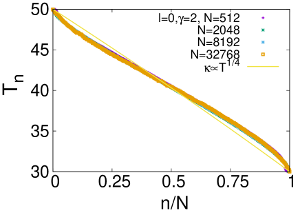
Figure 7: Temperature profile at c-FPU-$\beta$ at $l=0,\gamma=2,T_{L}=50,T_{R}=30\,\,(T_{L(R)}:$ left (right) reservoir temperature ). The corresponding curve of normal heat conduction $\kappa\propto T^{1/4}$ is also shown in the same figure. There are the cusps at the edges corresponding to the anomaly but the gaps at the edges cannot be seen. The clear systematic deviation means the asymptotics of the anomaly realized in this parameter region.

We begin by seeing that the scale-invariant form of the anomaly can appear at $l=0$ even in $\gamma=2,\Delta T/\bar{T}=0.5$ ($\Delta T$: temperature difference between two reservoirs). Figure 7 is the temperature profile at the parameters ($\gamma=2,\Delta T/\bar{T}=0.5,l=0$). The $n$-th particle’s temperature $T_{n}$ is defined by the kinetic temperature with the long time average. One can see the existence of the scale-invariant form

$$T_{n}=\tilde{T}_{l=0}(n/N).$$ (120)

($N$: system size.) As known, The heat conductivity shows power law temperature dependence $\kappa\propto T^{1/4}$ if one takes the temperature difference sufficiently small Aoki and Kusnezov (2001) in this parameter $l=0$. If the system recovers the normal heat condution with the power law temperature dependence of heat conductivity $\kappa\propto T^{a}$, their corresponding temperature profile must be described as $m\leq n\leq N-m,$

$$T_{n}=\left[T_{1+m}^{a+1}+(T_{N-m}^{a+1}-T_{1+m}^{a+1})\frac{n-m}{N-2m}\right]^{\frac{1}{a+1}},$$ (121)

but one cannot see the convergence to it in the figure. ($m$: the number of reservoir-attached particles to each reservoir.) There are increase of the gradient (cusps) around the edges (besides the gaps at the edges). This is a characteristic feature of the anomalous heat conduction and is caused by the growth of the correlation length. The position-dependent Green Kubo formula (at the position $n$) is proportional to $\int dt\sum_{i}\langle j_{n+1,n}j_{i+1,i}\rangle^{lc}$ ($\langle\rangle^{lc}$:local canonical averange defined in the precedeing appendix), so this is understood as the consequence of the fact that the integration range of the position becomes smaller than the correlation length $(\sim N)$ van Beijeren (2012). Here $j_{i+1,i}$ is the energy current between the $i+1,i$-th particles. Then this systematic deviation corresponds to the anomaly. Now the temperature gaps at the edges vanish. Only the cusps remain.

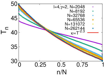
Figure 8: Temperature profile at c-FPU-$\beta$ at $l=4,\gamma=2,T_{L}=50,T_{R}=30$. The corresponding curve of normal heat conduction $\kappa\propto T^{-2.3}$ is also shown in the same figure. The clear convergence means the realization of the asymptotic form in this system. The gaps at the edges vanish at larger sizes.

Next, we checked whether the system at $l=4$ reaches the asymptotics (FIG 8). Before the discussion, we note that there are temperature gaps at smaller sizes, but the relation proposed by Aoki & Kusnezov (121) Aoki and Kusnezov (2002) can be used even in the situations. Then, seeing the profile at small sizes $N=2048,8192,32768$, one can find the increase of the gradient (cusps) at the edges, that corresponds to the anomaly. It means that there are actually the anomaly in this system at small sizes. The graph $\bar{\kappa}-N$ (FIG 2) actually has the region that shows the anomaly $\bar{\kappa}\sim N^{1/3}$ and the region just corresponds to the sizes we found here. After the checking, please see the convergence to the asymptotic curve as the gaps decrease. The profile that was straight at $N=8192$ has slowly bent and converges to the master curve $\kappa\propto T^{-2.3}$ of normal heat conduction at $N=131072,262144$. We put the curve of normal heat conduction $\kappa\propto T^{-2.3}$ with $T_{m+1}=49.7,T_{N-m}=30.3$. It is clear that it converges to the profile of the normal heat conduction. At least, one can understand that this behavior is not the artifact that merely cuts the pre-asymptotics only. The gaps vanish at larger sizes and one can safely use the Green Kubo formula in this case.

References

- De Groot and Mazur (2013) S. R. De Groot and P. Mazur, Non-equilibrium thermodynamics (Courier Corporation, 2013).
- Lepri et al. (2003) S. Lepri, R. Livi, and A. Politi, Physics Reports 377, 1 (2003).
- Dhar (2008) A. Dhar, Advances in Physics 57, 457 (2008).
- Lepri et al. (2015) S. Lepri, R. Livi, and A. Politi, arXiv preprint arXiv:1510.07844 (2015).
- Rieder et al. (1967) Z. Rieder, J. Lebowitz, and E. Lieb, Journal of Mathematical Physics 8, 1073 (1967).
- Casati et al. (1984) G. Casati, J. Ford, F. Vivaldi, and W. M. Visscher, Physical review letters 52, 1861 (1984).
- Prosen and Robnik (1992) T. Prosen and M. Robnik, Journal of Physics A: Mathematical and General 25, 3449 (1992).
- Matsuda and Ishii (1970) H. Matsuda and K. Ishii, Progress of Theoretical Physics Supplement 45, 56 (1970).
- Rubin and Greer (1971) R. J. Rubin and W. L. Greer, Journal of Mathematical Physics 12, 1686 (1971).
- O’Connor and Lebowitz (1974) A. O’Connor and J. Lebowitz, Journal of Mathematical Physics 15, 692 (1974).
- Narayan and Ramaswamy (2002) O. Narayan and S. Ramaswamy, Physical review letters 89, 200601_1 (2002).
- Dhar (2001) A. Dhar, Physical review letters 86, 5882 (2001).
- Kundu et al. (2010) A. Kundu, A. Chaudhuri, D. Roy, A. Dhar, J. L. Lebowitz, and H. Spohn, EPL (Europhysics Letters) 90, 40001 (2010).
- Saito and Dhar (2010) K. Saito and A. Dhar, Physical review letters 104, 040601 (2010).
- Spohn (2015) H. Spohn, arXiv preprint arXiv:1505.05987 (2015).
- Lepri et al. (1997) S. Lepri, R. Livi, and A. Politi, Physical review letters 78, 1896 (1997).
- Hatano (1999) T. Hatano, Physical Review E 59, R1 (1999).
- Savin et al. (2002) A. V. Savin, G. P. Tsironis, and A. V. Zolotaryuk, Physical review letters 88, 154301 (2002).
- Mai et al. (2007) T. Mai, A. Dhar, and O. Narayan, Physical review letters 98, 184301 (2007).
- Chang et al. (2008) C.-W. Chang, D. Okawa, H. Garcia, A. Majumdar, and A. Zettl, Physical review letters 101, 075903 (2008).
- Landau and Lifshitz (1987) L. Landau and E. Lifshitz, “Fluid mechanics (; oxford),” (1987).
- Grassberger et al. (2002) P. Grassberger, W. Nadler, and L. Yang, Physical review letters 89, 180601 (2002).
- Mendl and Spohn (2013) C. B. Mendl and H. Spohn, Physical review letters 111, 230601 (2013).
- Das et al. (2014a) S. G. Das, A. Dhar, K. Saito, C. B. Mendl, and H. Spohn, Physical Review E 90, 012124 (2014a).
- Kardar et al. (1986) M. Kardar, G. Parisi, and Y.-C. Zhang, Physical Review Letters 56, 889 (1986).
- Mendl and Spohn (2015) C. B. Mendl and H. Spohn, Journal of Statistical Mechanics: Theory and Experiment 2015, P03007 (2015).
- Kawasaki and Oppenheim (1965) K. Kawasaki and I. Oppenheim, Physical Review 139, A1763 (1965).
- Pomeau and Resibois (1975) Y. Pomeau and P. Resibois, Physics Reports 19, 63 (1975).
- Forster et al. (1977) D. Forster, D. R. Nelson, and M. J. Stephen, Physical Review A 16, 732 (1977).
- Mai and Narayan (2006) T. Mai and O. Narayan, Physical Review E 73, 061202 (2006).
- Hu et al. (2000) B. Hu, B. Li, and H. Zhao, Physical Review E 61, 3828 (2000).
- Bricmont and Kupiainen (2007) J. Bricmont and A. Kupiainen, Physical review letters 98, 214301 (2007).
- Pereira and Falcao (2006) E. Pereira and R. Falcao, Physical review letters 96, 100601 (2006).
- Lepri et al. (1998) S. Lepri, R. Livi, and A. Politi, EPL (Europhysics Letters) 43, 271 (1998).
- Kubo et al. (2012) R. Kubo, M. Toda, and N. Hashitsume, Statistical physics II: nonequilibrium statistical mechanics, Vol. 31 (Springer Science & Business Media, 2012).
- Gendelman and Savin (2000) O. V. Gendelman and A. V. Savin, Physical review letters 84, 2381 (2000).
- Giardinà et al. (2000) C. Giardinà, R. Livi, A. Politi, and M. Vassalli, Physical review letters 84, 2144 (2000).
- Das and Dhar (2014) S. G. Das and A. Dhar, arXiv preprint arXiv:1411.5247 (2014).
- Zhong et al. (2011) Y. Zhong, Y. Zhang, J. Wang, and H. Zhao, arXiv preprint arXiv:1107.3306 (2011).
- Chen et al. (2012) S. Chen, Y. Zhang, J. Wang, and H. Zhao, arXiv preprint arXiv:1204.5933 (2012).
- Savin and Kosevich (2014) A. V. Savin and Y. A. Kosevich, Physical Review E 89, 032102 (2014).
- Das et al. (2014b) S. G. Das, A. Dhar, and O. Narayan, Journal of Statistical Physics 154, 204 (2014b).
- Gendelman and Savin (2014) O. V. Gendelman and A. V. Savin, EPL (Europhysics Letters) 106, 34004 (2014).
- Wang et al. (2013) L. Wang, B. Hu, and B. Li, Physical Review E 88, 052112 (2013).
- Di Cintio et al. (2015) P. Di Cintio, R. Livi, H. Bufferand, G. Ciraolo, S. Lepri, and M. J. Straka, arXiv preprint arXiv:1509.08796 (2015).
- Chen et al. (2014) S. Chen, J. Wang, G. Casati, and G. Benenti, Physical Review E 90, 032134 (2014).
- Note (1) In the sense that the maximum Lyapunov exponent is large compared with dilute case () and the Lyapunov spectra shows the same shape with high energy FPU-, which correspond to the case that the Hessian of Hamiltonian is able to be replaced by the random matrix Newman (1986) on the surface spanned by conserved quantities.
- Bou-Rabee and Owhadi (2010) N. Bou-Rabee and H. Owhadi, SIAM Journal on Numerical Analysis 48, 278 (2010).
- Note (2) This is a prefetch but one cannot see the gradient increasing at the edges in this case, which is a characteristic feature of anomalous systems van Beijeren (2012).
- van Beijeren (2012) H. van Beijeren, Physical review letters 108, 180601 (2012).
- Hurtado and Garrido (2015) P. I. Hurtado and P. L. Garrido, arXiv preprint arXiv:1506.03234 (2015).
- Aoki and Kusnezov (2001) K. Aoki and D. Kusnezov, Physical review letters 86, 4029 (2001).
- Casati and Prosen (2003) G. Casati and T. Prosen, Physical Review E 67, 015203 (2003).
- Seifert (2012) U. Seifert, Reports on Progress in Physics 75, 126001 (2012).
- Eyring (1935) H. Eyring, The Journal of Chemical Physics 3, 107 (1935).
- Spohn (2014) H. Spohn, Journal of Statistical Physics 154, 1191 (2014).
- Drossel and Kardar (2002) B. Drossel and M. Kardar, Physical Review B 66, 195414 (2002).
- Lutsko and Dufty (2002) J. F. Lutsko and J. W. Dufty, Physical Review E 66, 041206 (2002).
- Kittel (2005) C. Kittel, Introduction to solid state physics (Wiley, 2005).
- Li et al. (2015) Y. Li, S. Liu, N. Li, P. Hänggi, and B. Li, New Journal of Physics 17, 043064 (2015).
- Kosevich and Savin (2015) Y. A. Kosevich and A. V. Savin, arXiv preprint arXiv:1509.03219 (2015).
- Lepri et al. (2005) S. Lepri, P. Sandri, and A. Politi, The European Physical Journal B-Condensed Matter and Complex Systems 47, 549 (2005).
- Bedeaux and Mazur (1974) D. Bedeaux and P. Mazur, Physica 73, 431 (1974).
- Maes and Netočnỳ (2010) C. Maes and K. Netočnỳ, Journal of Mathematical Physics 51, 015219 (2010).
- Itami and Sasa (2015) M. Itami and S.-i. Sasa, Journal of Statistical Physics 158, 37 (2015).
- Li et al. (2004) B. Li, L. Wang, and G. Casati, Physical review letters 93, 184301 (2004).
- Aoki and Kusnezov (2002) K. Aoki and D. Kusnezov, Annals of Physics 295, 50 (2002).
- Newman (1986) C. M. Newman, Communications in Mathematical Physics 103, 121 (1986).