Entropy production and large deviation function for systems with microscopically irreversible transitions

Abstract

We obtain the large deviation function for entropy production of the medium and its distribution function for two-site totally asymmetric simple exclusion process (TASEP) and three-state unicyclic network. Since such systems are described through microscopic irreversible transitions, we obtain time-dependent transition rates by sampling the states of these systems at a regular short time interval $\tau$. These transition rates are used to derive the large deviation function for the entropy production in the nonequilibrium steady state and its asymptotic distribution function. The shapes of the large deviation function and the distribution function depend on the value of the mean entropy production rate which has a non-trivial dependence on the particle injection and withdrawal rates in case of TASEP. Further, it is argued that in case of a TASEP, the distribution function tends to be like a Poisson distribution for smaller values of particle injection and withdrawal rates.

1 Introduction

The entropy production of the surrounding medium of a system driven out of equilibrium is arguably the most convenient tool for quantifying the irreversiblity. In the long time limit when the steady state value of the entropy production arising due to the boundary contributions could be neglected, the probability distribution function $P(\Delta S_{m},t)$ for the change in the medium entropy $\Delta S_{m}$ at time $t$, is known to satisfy certain symmetry relation, generally known as the fluctuation theorem evans1 ; gcsymm1 ; gcsymm2 ; kurchan ; lebowitz ; harris :

$$\frac{P(\Delta S_{m},t)}{P(-\Delta S_{m},t)}=\lim_{t\rightarrow\infty}e^{\Delta S_{m}}.$$ (1)

This symmetry relation implies that the probability of observing the entropy annihilation over a long time interval becomes negligibly small and can be viewed as the nonequilibrium generalization of the second law of thermodynamics. The derivation of the distribution function in the asymptotic time limit is often performed by finding out the corresponding large deviation function(LDF) $I(\Delta S_{m})$ which is related to the distribution function as,

$$I(\Delta S_{m})\equiv\lim_{t\rightarrow\infty}-\frac{1}{t}\ln P(\Delta S_{m},t).$$ (2)

The LDF plays the role of the free energy functions in equilibrium systems ellis ; touchette and in the case of nonequilibrium systems, its symmetry property, $I(-\Delta S_{m})=I(\Delta S_{m})+\Delta S_{m}/t$, validates the fluctuation theorem or the Gallavotti-Cohen symmetry gcsymm1 ; gcsymm2 ; kurchan ; lebowitz ; harris .

For a system described by the continuous time Markov dynamics, a microscopic transition from its configuration $i$ to $j$ with a transition rate, $\omega_{ij}$, causes the entropy of the surrounding medium to change lebowitz ; harris ; schn ; jchemphys ; seifert2 ; seifert3 by the amount $\Delta S_{m}=\ln\left(\frac{\omega_{ij}}{\omega_{ji}}\right)$, where $k_{B}$, the Boltzmann constant, is assumed to be unity. Of the many studies on the entropy production of the medium for systems with microscopic reversibility seifert2 ; seifert3 ; imparato ; rkpzia ; barato ; pleimling2 , some recent works on the properties of the LDF and its symmetry relation can be found in imparato ; pleimling2 where the authors studied the asymptotic distributions of the entropy production by finding out the LDF using a generating function based approach. In reference pleimling2 , the authors obtained the LDF for partially asymmetric simple exclusion processes and reaction-diffusion processes with microscopic reversibility. The emergence of a kink-like feature in the LDF at zero entropy production was argued to be generic for such processes. This kink could be characterized by the average value of the medium entropy production rate, making the entropy production rate a good candidate for quantifying the irreversibility in nonequilibrium systems.

While there is a wide applicability of the above formula for finding the medium entropy production for nonequilibrium systems having bi-directional transitions between its various states, this formula cannot be applied directly when we encounter a system with irreversible microscopic transitions between its states zeraati . Totally asymmetric simple exclusion processes(TASEP) where particles move in only one direction respecting the exclusion principle is one such example of systems with irreversible microscopic transition. Other examples include enzymatic reaction networks modeled by Michaelis-Menten scheme, directed percolation etc. In these systems when some of the transition rates $\omega_{ij}$ become zero, this formula predicts an infinite entropy production which have not been observed in realistic situations oliveira ; takeuchi . To address this shortcoming, ben-Avraham et al. pleimling1 proposed a regularization scheme by sampling the states of the system at small time interval and obtained the modified transition probabilities. Using those transition probabilities, they computed the medium entropy production rate and its LDF for a three-state irreversible loop. In reference zeraati , the authors used a slightly different method by introducing small backward transitions and determined the lower bound for the average rate of medium entropy production originating from the predominant irreversible transitions.

In this paper, we obtain the effective time-dependent transition rates for systems with irreversible transitions by allowing the systems to undergo all possible allowed transitions over small time interval $\tau$ and, then, deriving the probabilities of transition between any two states at the end of the time interval, $\tau$. The new transition rates are identical to the original transition rates for small $\tau$. These transition rates allow us to extend straightforwardly the generating function based approach used earlier lebowitz ; imparato to find out the LDF for the mean entropy production for irreversible systems. For a two-site TASEP and a three-state irreversible system, we first obtain the transition probabilities between any two arbitrary states by solving the governing Master equations. The transition rates are obtained after keeping the leading order terms in $\tau$ in the Taylor expansion of the time-dependent probabilities and then differentiating with respect to $\tau$. These new rates are used to obtain the average rate of medium entropy production and further to obtain the LDF for the entropy production through a saddle point approximation. At zero entropy production, the LDFs for both the models show a kink which can be characterized by the average entropy production rate mehl ; pleimling1 ; pleimling2 ; speck_t . Finally, the LDF is used to find the distribution of the entropy production in the long time limit. In the case of a two-site TASEP, the average rate of medium entropy production monotonically increases with the particle injection and withdrawal rates $\alpha$. For large values of the medium entropy production rate, the distribution function for the entropy production appears like a Gaussian distribution. For low entropy production rates, the distribution function turns out to be a non-Gaussian one. The features of the LDF that are responsible for producing the non-Gaussian shape of the entropy distribution function are strongly (exponentially) suppressed in the case of large entropy production rates.

The rest of the paper is organized as follows. In section 2, we introduce the entropy production formalisms for Markov jump processes and a practical way to apply those for systems having unidirectional transitions. In section 3, we first compute the rate of medium entropy production in the nonequilibrium steady state for two-site TASEP with equal injection and withdrawal rates denoted by $\alpha$. Next, we obtain the LDF as well as the distribution function for the medium entropy production for different values of $\alpha$. In section 4, using the same lines of approach, we obtain the analytical form of the LDF for entropy production for a three-state irreversible loop. The results are summarized in section 5.

2 Systems with irreversible transitions

In this section, we first present a brief overview of these relations schn ; lebowitz ; harris ; jchemphys ; seifert2 ; seifert3 ; tome valid for stochastic dynamics modeled as continuous time Markovian dynamics with finite, discrete configuration space. Next, we elucidate the feasibility of using the known entropy production formulae for a system having one or more microscopically irreversible transitions between its finite number of discrete states. Due to the microscopic irreversibility inherent in the system, some of the transition rates involved in the entropy production formulations are zero. Here, without introducing negligibly small backward transition rates as was done in rkpzia ; zeraati , we obtain the new set of transition rates by sampling the states of the system at a small time interval $\tau$. In the limit $\tau\rightarrow 0$, these new transition rates approach their original values, thus making the computations of entropy production rate and its LDF more accurate.

2.1 Entropy productions for Markov jump processes

We consider a continuous-time Markov jump process, for the time interval $0\leq t\leq t_{f}$, with finite number of states. The dynamical evolution of the probability $P_{i}(t)$, that the system is found in state $i$, is described by the Master equation

$$\frac{\partial}{\partial t}P_{i}(t) = \sum_{j\neq i}\left(\omega_{ji}(t)P_{j}(t)-\omega_{ij}(t)P_{i}(t)\right)$$ (3)

$$= \sum_{j}T_{ij}P_{j},$$

where $\omega_{ji}$ and $\omega_{ij}$ are the transition rates for the jump from state $j$ to $i$ and from state $i$ to $j$, respectively. Equation(3) can be written in matrix form as,

$$\frac{\partial}{\partial t}\mathbf{P}(t)=\mathbf{T}\mathbf{P}(t),$$ (4)

where $\mathbf{P}=(P_{1},P_{2},\dots)^{T}$ is the column matrix and the $\{i,j\}$th element of the transition matrix $\mathbf{T}$ are

$$T_{ij}=\omega_{ji}-\delta_{ij}\sum_{k\neq i}\omega_{ik}.$$ (5)

In order to obtain the expression for the entropy production due to a transition from one state to another, we begin by defining the average Gibbs entropy of the system as

$$\langle S\rangle=-\sum_{i}P_{i}\ln P_{i}.$$ (6)

The expression for the time evolution of the system entropy has the form (schn, ; lebowitz, ; harris, ; jchemphys, ; seifert2, ; seifert3, ; tome, )

$$\langle\dot{S}\rangle=\sum_{i,j}P_{i}\omega_{ij}\ln\left(\frac{P_{i}\omega_{ij}}{P_{j}\omega_{ji}}\right)-\sum_{i,j}P_{i}\omega_{ij}\ln\left(\frac{\omega_{ij}}{\omega_{ji}}\right),$$ (7)

where the overdot implies a derivative with respect to time. The first term on the right hand side of the above relation is always positive and is identified as the total entropy production rate due to stochastic transitions. The second term is the medium entropy production rate or the entropy flow into the medium due to these transitions. The total rate of the entropy production is now expressed as

$$\langle\dot{S}_{tot}\rangle=\langle\dot{S}\rangle+\langle\dot{S}_{m}\rangle,$$ (8)

with

$$\langle\dot{S}_{tot}\rangle=\sum_{i,j}P_{i}\omega_{ij}\ln\left(\frac{P_{i}\omega_{ij}}{P_{j}\omega_{ji}}\right)\ \ {\rm and}\ \ \langle\dot{S}_{m}\rangle=\sum_{i,j}P_{i}\omega_{ij}\ln\left(\frac{\omega_{ij}}{\omega_{ji}}\right).$$ (9)

2.2 Computations of time-dependent transition rates

In order to calculate the medium entropy production rate, we first briefly describe the strategy to compute the transition rates employing a matrix-based approach. To begin with, we consider a Markov process in which transitions between the discrete states $i=(1,2,\dots N)$ are measured in discrete time steps, $t=n\Delta t$, where $n=0,1,2\dots$. The solution of equation(4) is determined by diagonalizing the matrix $\mathbf{T}$ as $\mathbf{T_{D}}=\mathbf{B}^{-1}\cdot\mathbf{T}\cdot\mathbf{B}$, where matrix $\mathbf{B}$ is formed of the eigenvectors of $\mathbf{T}$ arranged column-wise, and $\mathbf{B}^{-1}$ is the inverse of $\mathbf{B}$. The diagonal matrix $\mathbf{T_{D}}$ has the eigenvalues of $\mathbf{T}$ as its diagonal elements. The solution of equation(4) then reads

$$\mathbf{P}(t)=\mathbf{B}\cdot e^{t\mathbf{T_{D}}}\cdot\mathbf{B}^{-1}\cdot\mathbf{P}(0)=\mathbf{\bar{T}}\cdot\mathbf{P}(0).$$ (10)

The elements of the $\mathbf{\bar{T}}$ matrix are the transition probabilities. For instance, the element $\bar{T}_{ij}$, in conventional notation, implies $\bar{T}(i,t|j,0)$, i.e., the probability of finding the system at $i$-th state at time $t$, provided it was at $j$-th state at the initial time. These transition probabilities allow us to obtain the time-dependent transition rates reichl if the states of the system are sampled at small time interval $\Delta t$. To be more specific, let us consider the probability $P_{i}(t+\Delta t)$ at time $t+\Delta t$ of finding the system at state $i$. In the limit $\Delta t\rightarrow 0$, we have,

$$P_{i}(t+\Delta t)\approx P_{i}(t)+\Delta t\frac{\partial}{\partial t}P_{i}(t)$$

$$=P_{i}(t)+\Delta t\sum_{j}W_{ij}P_{j}(0).$$ (11)

This relation defines $W_{ij}$ which denotes the transition rate from state $j$ to $i$. In the subsequent sections, these transition rates are used in relation (9) to calculate the average rate of entropy production of the medium, its LDF and the distribution function in the asymptotic time limit.

3 Entropy production for two-site TASEP

3.1 Time-dependent transition rates

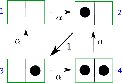
Figure 1: Four states with the transition rates for two-site TASEP.

We consider two-site TASEP with equal particle injection and withdrawal rates $\alpha$ as our first model of a system with irreversible transitions between its four states as shown in figure 1. Let us consider the time evolution of the probability densities $\mathbf{P}=(P_{1},P_{2},P_{3},P_{4})^{T}$, where the element $P_{i}$ of the column matrix denotes the probability of finding the system in state $i$. The governing Master equation can be written as,

$$\frac{\partial}{\partial t}\mathbf{P}(t)=\mathbf{T}\mathbf{P}(t),$$ (12)

where $\mathbf{T}$ is the $4\times 4$ matrix having the following form,

$$\mathbf{T}=\left(\begin{array}[]{rrrr}-\alpha&0&\alpha&0\\ \alpha&-1&0&\alpha\\ 0&1&-2\alpha&0\\ 0&0&\alpha&-\alpha\\ \end{array}\right).$$ (13)

The eigenvalues of $\mathbf{T}$ are $\lambda_{1}=0,\ \lambda_{2}=-\alpha,\ \lambda_{3}=-\frac{1}{2}[1+3\alpha+\sqrt{1-6\alpha+\alpha^{2}}],\ \lambda_{4}=\frac{1}{2}[-1-3\alpha+\sqrt{1-6\alpha+\alpha^{2}}]$ with the corresponding eigenvectors

$$e_{1}=(1,2\alpha,1,1)^{T};\ e_{2}=(-1,0,0,1)^{T};\ e_{3}=\left(1,\frac{1}{2\alpha}[1-3\alpha+\sqrt{1-6\alpha+\alpha^{2}}],-\frac{1}{2\alpha}[1+\alpha+\sqrt{1-6\alpha+\alpha^{2}}],1\right)^{T};$$ (14)

$$e_{4}=\left(1,\frac{1}{2\alpha}[1-3\alpha-\sqrt{1-6\alpha+\alpha^{2}}],-\frac{1}{2\alpha}[1+\alpha-\sqrt{1-6\alpha+\alpha^{2}}],1\right)^{T}.$$ (15)

The matrix $\mathbf{B}^{-1}$ has the form

$$\mathbf{B}^{-1}=\frac{1}{3+2\alpha}\left(\begin{array}[]{cccc}1&1&1&1\\ -(3+2\alpha)/2&0&0&(3+2\alpha)/2\\ \frac{\alpha-1-2\alpha^{2}+m(1+2\alpha)}{4m}&\frac{1+3\alpha-m}{2m}&\frac{1-\alpha(3+4\alpha)-m}{2m}&\frac{\alpha-1-2\alpha^{2}+m(1+2\alpha)}{4m}\\ \frac{1-\alpha+2\alpha^{2}+m(1+2\alpha)}{4m}&\frac{-(1+3\alpha+m)}{2m}&\frac{\alpha(3+4\alpha)-1-m}{2m}&\frac{1-\alpha+2\alpha^{2}+m(1+2\alpha)}{4m}\\ \end{array}\right),$$ (20)

with $m=\sqrt{1+\alpha(\alpha-6)}$.

Substituting $\mathbf{B}$, $\mathbf{T}_{D}$ and $\mathbf{B}^{-1}$ in equation(10), each element of the column vector ${\bf P}(t)$ is expressed as

$$P_{i}(t)=\sum_{j}\bar{T}_{ij}P_{j}(0),$$ (21)

which can be written in the compact form as

$$\mathbf{P}(t)=\mathbf{\bar{T}}\mathbf{P}(0).$$ (22)

In the above equation, the conditional probability $\bar{T}_{ij}$ implies the probability of finding the system at $i$-th state at time $t$, provided it was at $j$-th state at initial time. $\bar{T}_{ii}$ term corresponds to the null transition. If we consider the time interval, $t=\tau$, to be small such that the sampling time becomes, $\tau<<1/\alpha$, it is then ensured that the transition matrix $\mathbf{W}$ becomes closer to the original transition matrix (13). In this limit, the matrix $\mathbf{\bar{T}}$ has the form,

$$\mathbf{\bar{T}}=\left(\begin{array}[]{cccc}1-\alpha\tau+\frac{\alpha^{2}\tau^{2}}{2}&\frac{\alpha\tau^{2}}{2}&\alpha\tau-\frac{3\alpha^{2}\tau^{2}}{2}&\frac{\alpha^{2}\tau^{3}}{6}\\ \alpha\tau-\frac{\alpha(1+\alpha)\tau^{2}}{2}&1-\tau+\frac{\tau^{2}}{2}&\alpha^{2}\tau^{2}&\alpha\tau-\frac{\alpha(1+\alpha)\tau^{2}}{2}\\ \frac{\alpha\tau^{2}}{2}&\tau-(\alpha+\frac{1}{2})\tau^{2}&1-2\alpha\tau+2\alpha^{2}\tau^{2}&\frac{\alpha\tau^{2}}{2}\\ \frac{\alpha^{2}\tau^{3}}{6}&\frac{\alpha\tau^{2}}{2}&\alpha\tau-\frac{3\alpha^{2}\tau^{2}}{2}&1-\alpha\tau+\frac{\alpha^{2}\tau^{2}}{2}\\ \end{array}\right).$$ (27)

The corresponding transition matrix $\mathbf{W}$ as defined in (11) is

$$\mathbf{W}=\left(\begin{array}[]{cccc}\alpha^{2}\tau-\alpha&\alpha\tau&\alpha-3\alpha^{2}\tau&\frac{\alpha^{2}\tau^{2}}{2}\\ \alpha-\alpha(1+\alpha)\tau&\tau-1&2\alpha^{2}\tau&\alpha-\alpha(1+\alpha)\tau\\ \alpha\tau&1-2(\alpha+\frac{1}{2})\tau&4\alpha^{2}\tau-2\alpha&\alpha\tau\\ \frac{\alpha^{2}\tau^{2}}{2}&\alpha\tau&\alpha-3\alpha^{2}\tau&\alpha^{2}\tau-\alpha\\ \end{array}\right).$$ (32)

3.2 Average entropy production rate of the medium

Having obtained the time-dependent transition rates in the previous subsection, we now evaluate the average rate of medium entropy production in the nonequilibrium steady state as defined in equation(9). We define the transition rate for a transition from state $j$ to $i$ as $\tilde{\omega}_{ji}$ which is related to the corresponding element of the transition matrix as, $\tilde{\omega}_{ji}=W_{ij}$. The steady state probability densities for the two-site model are obtained as,

$$P_{1s}=P_{3s}=P_{4s}=\frac{1}{3+2\alpha};\ \ \ \ P_{2s}=\frac{2\alpha}{3+2\alpha}.$$ (33)

In the small time limit, the ratio of the forward and the reverse transition rates are approximated as,

$$\frac{\tilde{\omega}_{12}}{\tilde{\omega}_{21}}\approx\frac{\tilde{\omega}_{31}}{\tilde{\omega}_{13}}\approx\frac{\tilde{\omega}_{42}}{\tilde{\omega}_{24}}\approx\frac{\tilde{\omega}_{34}}{\tilde{\omega}_{43}}\approx\frac{1}{\tau},$$ (34)

$$\frac{\tilde{\omega}_{23}}{\tilde{\omega}_{32}}\approx\frac{1}{2\alpha^{2}\tau}.$$ (35)

The average rate of entropy production of the medium is thus obtained as,

$$\langle\dot{S}_{m}\rangle = \sum_{i,j}P_{is}\tilde{\omega}_{ij}\ln\frac{\tilde{\omega}_{ij}}{\tilde{\omega}_{ji}}$$ (36)

$$= \frac{2\alpha(1-\tau-3\alpha\tau)}{(3+2\alpha)}\left[2\ln(1/\tau)+\ln(1/(2\alpha^{2}\tau))\right].$$

The entropy production rate is plotted in the figure 2(a) with $\alpha$. The positivity of the entropy production suggests that the medium entropy increases as the system undergoes transition from one state to another.

3.3 Large deviation function for entropy production and its distribution function

With the definition of the transition matrix $\mathbf{W}$ in the previous section, we calculate the LDF for entropy productionlebowitz ; imparato . Let $\phi_{i}(\Delta S_{m},t)$ be the probability that the system is in the $i$-th state at time $t$ while the change in the medium entropy is $\Delta S_{m}$. The probability of finding the system at time $t+\tau$ after a small time interval $\tau$, during which the entropy exchange with the medium is $\Delta s_{ji}=\ln\left(\frac{\tilde{\omega}_{ji}}{\tilde{\omega}_{ij}}\right)$ due to the jump of the system from state $j$ to $i$, is expressed as imparato ,

$$\phi_{i}(\Delta S_{m},t+\tau)\approx\phi_{i}(\Delta S_{m},t)+\tau\sum_{j}\left[\tilde{\omega}_{ji}\phi_{j}(\Delta S_{m}-\Delta s_{ji},t)-\tilde{\omega}_{ij}\phi_{i}(\Delta S_{m},t)\right].$$ (37)

In the limit $\tau\rightarrow 0$, we have,

$$\frac{\partial\phi_{i}}{\partial t}=\sum_{j}\left[\tilde{\omega}_{ji}\left(\sum_{n=0}^{\infty}\frac{(-\Delta s_{ji})^{n}}{n!}\frac{\partial^{n}}{\partial(\Delta S_{m})^{n}}\phi_{j}\right)-\tilde{\omega}_{ij}\phi_{i}\right].$$ (38)

Introducing the generating function

$$\psi_{i}(\lambda,t)=\int d(\Delta S_{m})e^{-\lambda\Delta S_{m}}\phi_{i},$$ (39)

we write the time evolution of the generating function as,

$$\frac{\partial\psi_{i}}{\partial t} = \sum_{j}\tilde{\omega}_{ji}\psi_{j}e^{-\lambda\Delta s_{ji}}-\sum_{j}\tilde{\omega}_{ij}\psi_{i}$$ (40)

$$= \sum_{j}\tilde{\omega}_{ji}^{1-\lambda}\tilde{\omega}_{ij}^{\lambda}\psi_{j}-\sum_{j}\tilde{\omega}_{ij}\psi_{i}=\sum_{j}L_{ij}\psi_{j}.$$

The above equation can be written in a matrix form as,

$$\frac{\partial{\bm{\psi}}}{\partial t}=\mathbf{L}{\bm{\psi}},$$ (41)

where

$$\mathbf{L}=\left(\begin{array}[]{llll}-(\alpha+\alpha^{2}\tau(\tau-2)/2)&(\alpha\tau)^{1-\lambda}(\alpha-\alpha(1+\alpha)\tau)^{\lambda}&(\alpha-3\alpha^{2}\tau)^{1-\lambda}(\alpha\tau)^{\lambda}&\frac{\alpha^{2}\tau^{2}}{2}\\ (\alpha-\alpha(1+\alpha)\tau)^{1-\lambda}(\alpha\tau)^{\lambda}&\tau-1&(2\alpha^{2}\tau)^{1-\lambda}[1-2(\alpha+0.5)\tau]^{\lambda}&(\alpha-\alpha(1+\alpha)\tau)^{1-\lambda}(\alpha\tau)^{\lambda}\\ (\alpha\tau)^{1-\lambda}(\alpha-3\alpha^{2}\tau)^{\lambda}&(1-2(\alpha+0.5)\tau)^{1-\lambda}(2\alpha^{2}\tau)^{\lambda}&(4\alpha^{2}\tau-2\alpha)&(\alpha\tau)^{1-\lambda}(\alpha-3\alpha^{2}\tau)^{\lambda}\\ \frac{\alpha^{2}\tau^{2}}{2}&(\alpha\tau)^{1-\lambda}(\alpha-\alpha(1+\alpha)\tau)^{\lambda}&(\alpha-3\alpha^{2}\tau)^{1-\lambda}(\alpha\tau)^{\lambda}&-(\alpha+\alpha^{2}\tau(\tau-2)/2)\\ \end{array}\right),$$ (46)

and ${\bm{\psi}}=(\psi_{1},\psi_{2},\psi_{3},\psi_{4})^{T}$.

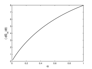
(a) (b)

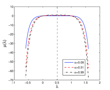
Figure 2: (a) Rate of average entropy production of the medium. The value of the small time interval, $\tau=0.001$. (b) The smallest eigenvalue, $\mu(\lambda)$, for different values of particle injection/withdrawal rates $\alpha$. For smaller values of $\alpha$, it becomes more flat around $\mu=0$. The symmetry about the vertical dashed line at $\lambda=0.5$ is the manifestation of the fluctuation theorem.

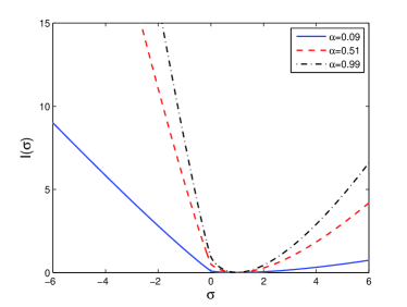
(a) (b)

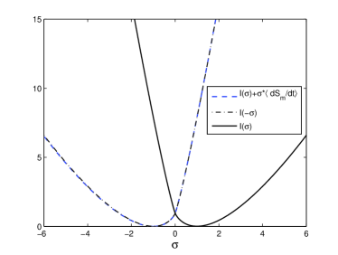
Figure 3: (a) Large deviation function for the scaled entropy production $\sigma$ for different values of particle injection and withdrawal rates, $\alpha$. The kink like feature in the LDF at zero entropy production becomes more prominent for larger values of $\alpha$. The blue solid line, the red dashed line and the black dashed-dot line correspond to the values of the average rate of entropy production $1.379,5.389,\textrm{and}\ 7.911$ respectively. (b) This figure displays the validity of the symmetry relation, $I(\sigma)+\langle\dot{S}_{m}\rangle\sigma=I(-\sigma)$, satisfied by the LDF. The dashed line and the dashed-dot line have merged completely in the figure.

In order to find the total probability distribution $\phi(\Delta S_{m},t)=\sum_{i}\phi_{i}(\Delta S_{m},t)$, we need to introduce the total generating function $\psi(\lambda,t)=\sum_{i}\psi_{i}(\lambda,t)$. In the large time limit, the total generating function can be approximated as,

$$\psi(\lambda)\approx\lim_{t\rightarrow\infty}\exp(-t\mu_{0}(\lambda)),$$ (47)

where $\mu_{0}(\lambda)$ is the smallest of all the eigenvalues defined through the following equation

$$\mathbf{L}\mathbf{l_{n}}(\lambda)=-\mu_{n}(\lambda)\mathbf{l_{n}}(\lambda).$$ (48)

We evaluate the smallest eigenvalue numerically and it is plotted in figure 2(b) with $\lambda$. The symmetry of the smallest eigenvalue about $\lambda=0.5$ validates the fluctuation theorem $\mu_{0}(\lambda)=\mu_{0}(1-\lambda)$ gcsymm1 ; gcsymm2 ; kurchan ; lebowitz ; harris . The average rate of entropy production of the medium $\langle\dot{S}_{m}\rangle$ is related to the smallest eigenvalue as,

$$\left\langle\dot{S}_{m}\right\rangle=\frac{\partial\mu_{0}(\lambda)}{\partial\lambda}|_{\lambda=0}.$$ (49)

In order to obtain the probability distribution $\phi_{i}(\Delta S_{m},t)$, one has to invert the relation in equation (39). The final integration is done using a saddle point approximation scheme. The LDF or the rate function $I(\sigma)$ with $\sigma=\frac{\Delta S_{m}}{t\left\langle\dot{S}_{m}\right\rangle}$ as the normalised rate of entropy production, can be expressed as the Legendre transform of $\mu_{0}(\lambda)$

$$I(\sigma)=\mu_{0}(\lambda^{*})-\lambda^{*}\sigma\left\langle\dot{S}_{m}\right\rangle.$$ (50)

Here $\lambda^{*}$ is the saddle point defined through the equation $\frac{\partial\mu_{0}(\lambda)}{\partial\lambda}|_{\lambda^{*}}=\sigma\left\langle\dot{S}_{m}\right\rangle$. From figure 2(a), it is evident that the average entropy production rate is always positive and it increases as we increase the value of $\alpha$. At zero entropy production, the LDF shows a kink which becomes prominent for larger values of $\alpha$ (see figure 3(a)). The symmetry property displayed by the LDF, $I(\sigma)+\langle\dot{S}_{m}\rangle\sigma=I(-\sigma)$, as shown in figure 3(b), is attributed to the symmetry property of the distribution function of entropy production quantified through the fluctuation theorem.

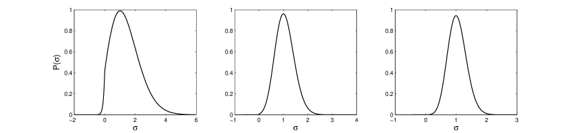
Figure 4: Probability distribution for the scaled entropy production at time $t=10$. From the left to right panel, the three figures correspond to the rates $\alpha=0.09$, $\alpha=0.51$ and $\alpha=0.99$, respectively. For the small values of the entry and exit rates, the distribution is non-Gaussian. The distribution tends to be Gaussian for larger values of entry and exit rates.

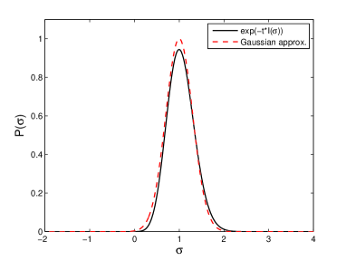
Figure 5: Probability distribution for the scaled entropy production at time $t=10$ for $\alpha=0.99$. For this value of $\alpha$, $\langle\dot{S}_{m}\rangle=7.911$. The solid black curve corresponds to the $\exp(-t*I(\sigma))$ and the red dashed curve is obtained using equation(52).

Using the expression for the LDF, one may find out the probability distribution function of the normalized entropy production rate $P(\sigma)$ in the asymptotic time limit as

$$P(\sigma)\sim\lim_{t\rightarrow\infty}\exp(-tI(\sigma)).$$ (51)

The LDF provides the detailed information about the distribution function, which is non-Gaussian in nature in our case, for large fluctuations. However, for larger values of $\alpha$ when the value of the average entropy production rate is also large, the central part of the distribution tends to be Gaussian, while for smaller values of $\alpha$ it has a non-Gaussian form. Intuitively, for small $\alpha$, the number of transitions are also small and over the time interval $t=10$, the smaller number of events cause the distribution function to have a Poisson distribution-like form. The distribution functions $P(\sigma)$ for three different values of $\alpha$ are plotted in figure 4.

To have a qualitative understanding of the distribution function for larger values of $\langle\dot{S}_{m}\rangle$, it should be noted from figure 3(a) that the values of the LDF from its minimum are larger if the rate of medium entropy production is increased. These large fluctuations are strongly suppressed in the exponential form of the distribution function. Thus, if we perform a Taylor expansion of the LDF about its minimum at $\sigma=1$, we have

$$I(\sigma)\approx\frac{1}{2}\frac{d^{2}I(\sigma)}{d\sigma^{2}}|_{\sigma=1}(\sigma-1)^{2}.$$ (52)

We determine the second derivative numerically and for $\langle\dot{S}_{m}\rangle=7.911$, its value is, $\frac{d^{2}I(\sigma)}{d\sigma^{2}}|_{\sigma=1}=1.101$. Taking the form of $I(\sigma)$ as in the equation(52), we obtain the distribution function for large values of medium entropy production (see figure 5). The matching between the original distribution and the approximated one is remarkable and thus, the distribution can be approximated as Gaussian for large $\langle\dot{S}_{m}\rangle$. However, similar approximation cannot be made for smaller values of $\langle\dot{S}_{m}\rangle$ since in this case, the fluctuations away from the center are not so large. This explains why the distribution function in this case becomes non-Gaussian.

4 Three-state unicyclic network

Here we apply the present method to a three-state irreversible loop pleimling1 where the transitions between the three states denoted as $1,\ 2\ {\rm and}\ 3$ happen in a cyclic way as $1\rightarrow 2,\ 2\rightarrow 3,\ 3\rightarrow 1$ with rate $1$. In the small time interval $\tau$, the transition rates $\tilde{\omega}_{ij}$s have the form,

$$\tilde{\omega}_{12}=\tilde{\omega}_{23}=\tilde{\omega}_{31}\approx 1-2\tau,$$ (53)

$$\tilde{\omega}_{21}=\tilde{\omega}_{32}=\tilde{\omega}_{13}\approx\tau.$$ (54)

As before, the time evolution of the generating function $\psi_{i}$ $(i=1,2,3)$, as defined in equation(39), is governed by,

$$\frac{\partial{\bm{\psi}}}{\partial t}=\mathbf{L}{\bm{\psi}},$$ (55)

where ${\bm{\psi}}=(\psi_{1},\psi_{2},\psi_{3})^{T}$ and $\mathbf{L}$ has the form,

$$\mathbf{L}=\left(\begin{array}[]{lll}\tau-1&(1-2\tau)^{\lambda}\tau^{1-\lambda}&(1-2\tau)^{1-\lambda}\tau^{\lambda}\\ (1-2\tau)^{1-\lambda}\tau^{\lambda}&\tau-1&(1-2\tau)^{\lambda}\tau^{1-\lambda}\\ (1-2\tau)^{\lambda}\tau^{1-\lambda}&(1-2\tau)^{1-\lambda}\tau^{\lambda}&\tau-1\\ \end{array}\right).$$ (59)

The smallest eigenvalue of ${\bf L}$ dominates the large time behavior of the total generating function $\psi=\sum_{i}\psi_{i}$. In this case, the smallest eigenvalue is

$$\mu_{0}(\lambda)=1-\tau-(1-2\tau)^{\lambda}\tau^{1-\lambda}-(1-2\tau)^{1-\lambda}\tau^{\lambda}.$$ (60)

The rate of medium entropy production is found as,

$$\langle\dot{S}_{m}\rangle=\frac{\partial\mu_{0}}{\partial\lambda}|_{\lambda=0}=(1-3\tau)\ln[(1-2\tau)/\tau].$$ (61)

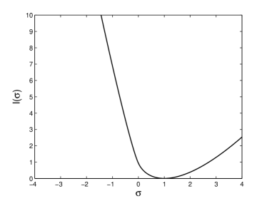
(a) (b)

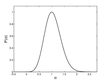
Figure 6: (a) Large deviation function for the scaled entropy production $\sigma$ for $\tau=0.001$. (b) Distribution of the scaled entropy production at time $t=10$.

The LDF for the normalized entropy production $\sigma=\Delta S_{m}/(t\langle\dot{S}_{m}\rangle)$ has the form

$$I(\sigma)=\mu_{0}(\lambda^{*})-\lambda^{*}\sigma\left\langle\dot{S}_{m}\right\rangle,$$ (62)

where the saddle point $\lambda^{*}$ is defined implicitly as

$$\tau^{\lambda^{*}}(1-2\tau)^{1-\lambda^{*}}-(1-2\tau)^{\lambda^{*}}\tau^{1-\lambda^{*}}=\sigma(1-3\tau).$$ (63)

Expressing equation (63) in terms of $x$, where $x=\tau^{\lambda^{*}}(1-2\tau)^{-\lambda^{*}}$, we find

$$x=\frac{\sigma(1-3\tau)+\sqrt{\sigma^{2}(1-3\tau)^{2}+4\tau(1-2\tau)}}{2(1-2\tau)}.$$ (64)

The saddle point $\lambda^{*}$ is related to $x$ as

$$\lambda^{*}=-(1-3\tau)\frac{\ln(x)}{\langle\dot{S}_{m}\rangle}.$$ (65)

Substituting equation(60), (61) and (65) into (62), we have

$$I(\sigma)=1-\tau-\frac{\tau}{x}-(1-2\tau)x+\sigma(1-3\tau)\ln(x).$$ (66)

The symmetry property of the LDF, $I(\sigma)-I(-\sigma)=-\langle\dot{S}_{m}\rangle\sigma$, implies that the fluctuation relation for the entropy production in the medium holds for the system in the long time limit. The plot of the LDF for the entropy production (see figure 6(a)) shows a kink at zero entropy production as a consequence of the fluctuation theorem pleimling1 ; pleimling2 . The distribution function for the entropy production, as shown in 6(b), is obtained directly from equation (66).

5 Summary and future perspectives

In summary, we have obtained the LDF and the probability distribution function for the medium entropy production for a two-site TASEP and a three-state cyclic process. Both TASEP and the three-state process involve irreversible transitions due to the hopping of particles in a specific direction and the unicyclic nature of the three-state process. In order to apply the general results of entropy production for stochastic jump processes, we obtained first the time-dependent transition rates by sampling the states of the systems over a short time interval. These new transition rates are incorporated in the subsequent derivations of the LDF for the entropy production which satisfies Gallavotti-Cohen symmetry. For the two-site TASEP, the value of the LDF for large fluctuations becomes higher as the average entropy production rate is increased. As a consequence of this, the distribution function tends to be Gaussian. For smaller values of particle injection and withdrawal rates, which in turn makes the average entropy production rate smaller, the distribution function becomes non-Gaussian and it resembles Poisson distribution because of lesser number of events over the time interval. For the three-state irreversible loop, we have found the analytical forms of the smallest eigenvalue and the LDF. For both the processes, the smallest eigenvalue and the LDF are derived keeping the first order terms in $\tau$ in the new transition rates. The smallest eigenvalue and the LDF for the medium entropy production satisfy the fluctuation theorem. Our results for the three-state process differ slightly from the previous study pleimling1 since we incorporate here the conventional definition of the transition rates in the subsequent derivations of the smallest eigenvalue and the LDF. In reference ohkubo , applying Bayes theorem to the posterior probabilities, it has been shown that the microscopic reversibility condition is not a necessity to propose a generalize fluctuation theorem for total entropy production. Since using time coarse-graining procedure, we obtain nonzero reverse transition probabilities even for processes involving irreversible transitions, it is expected that this procedure leads to holding symmetry relations of certain kinds for the probability distribution of entropy production. Using similar coarsening theorem, the authors in reference pleimling3 have shown the validity of integral fluctuation theorem and Crooks relation for Hatano-Sasa entropy of many-state irreversible processes. Finally, the present methodology based on derivation of the time-dependent transition rates seems to be useful for studying a broad range of models relevant to physical and biophysical processes including complex networks involving multiple degrees of freedom pleimling3 ; robert .

References

- (1) Evans D J, Cohen E G D and Morriss G P, 1993 Phys. Rev. Lett. 71 2401
- (2) Gallavotti G and Cohen E G D, 1995 Phys. Rev. Lett. 74 2694
- (3) Gallavotti G and Cohen E G D, 1995 J. Stat. Phys. 80 931
- (4) Kurchan J, 1998 J. Phys. A 31 3719
- (5) Lebowitz J L and Spohn H, 1999 J. Stat. Phys. 95 333
- (6) Harris R J and Schütz G M, 2007 J. Stat. Mech. P07020
- (7) Ellis R S, 1985 Entropy, Large Deviations, and Statistical Mechanics (Berlin: Springer)
- (8) Touchette H, 2009 Physics Reports 478 1
- (9) Schnakenberg J, 1976 Rev. Mod. Phys. 48 571
- (10) Andrieux D and Gaspard P, 2004 J. Chem. Phys. 121 6167
- (11) Seifert U, 2005 Phys. Rev. Lett. 95 040602
- (12) Seifert U, 2008 Eur. Phys. J. B 64 423
- (13) Tomé T and de Oliveira M J 2012 Phys. Rev. Lett. 108 020601
- (14) Zia R K P and Schmittmann B, 2007 J. Stat. Mech. P07012
- (15) Barato A C, Chetrite R, Hinrichsen H and Mukamel D, 2010 J. Stat. Mech. P10008
- (16) Imparato A and Peliti L, 2007 J. Stat. Mech. L02001
- (17) Dorosz S and Pleimling M, 2011 Phys. Rev. E 83 031107
- (18) de Oliveira Rodrigues J E and Dickman R, 2010 Phys. Rev. E 81 061108
- (19) Takeuchi K A, Kuroda M, Chaté H and Sano M, 2007 Phys. Rev. Lett. 99 234503
- (20) ben-Avraham D, Dorosz S and Pleimling M, 2011 Phys. Rev. E 84 011115
- (21) Zeraati S, Jafarpour F H and Hinrichsen H, 2012 J. Stat. Mech. L12001
- (22) Mehl J, Speck T and Seifert U, 2008 Phys. Rev. E 78 011123
- (23) Speck T, Engel A and Seifert U, 2012 J. Stat. Mech. P12001
- (24) Reichl L E, 1980 A Modern Course in Statistical Physics (Weinheim: Wiley-VCH)
- (25) Ohkubo J, 2009 J. Phys. Soc. Jpn. 78 123001
- (26) ben-Avraham D, Dorosz S and Pleimling M, 2011 Phys. Rev. E 83 041129
- (27) Gernert R, Emary C and Klapp S H L, 2014 Phys. Rev. E 90 062115