A New Relaxation Approach to Normalized Hypergraph Cut

Abstract

Normalized graph cut (NGC) has become a popular research topic due to its wide applications in a large variety of areas like machine learning and very large scale integration (VLSI) circuit design. Most of traditional NGC methods are based on pairwise relationships (similarities). However, in real-world applications relationships among the vertices (objects) may be more complex than pairwise, which are typically represented as hyperedges in hypergraphs. Thus, normalized hypergraph cut (NHC) has attracted more and more attention. Existing NHC methods cannot achieve satisfactory performance in real applications. In this paper, we propose a novel relaxation approach, which is called relaxed NHC (RNHC), to solve the NHC problem. Our model is defined as an optimization problem on the Stiefel manifold. To solve this problem, we resort to the Cayley transformation to devise a feasible learning algorithm. Experimental results on a set of large hypergraph benchmarks for clustering and partitioning in VLSI domain show that RNHC can outperform the state-of-the-art methods.

1 Introduction

The goal of graph cut (or called graph partitioning) Wu and Leahy (1993) is to divide the vertices (nodes) in a graph into several groups (clusters), making the number of edges across different clusters minimized while the number of edges within the clusters maximized. Besides the goal which should be achieved in graph cut, normalized graph cut (NGC) should also make the volumes of different clusters as balanced as possible by adopting some normalization techniques. In many real applications, NGC has been proved to achieve better performance than unnormalized graph cut Shi and Malik (2000); Ng et al. (2001); Gonzalez et al. (2012). Thus, NGC is a popular theme due to its wide applications in a large variety of areas, including machine learning Ng et al. (2001); Xie et al. (2014), parallel and distributed computation Gonzalez et al. (2012); Jain et al. (2013); Chen et al. (2015), image segmentation Shi and Malik (2000), and social network analysis Tang and Liu (2010); Li and Schuurmans (2011), and so on. For example, graph-based clustering methods such as spectral clustering Ng et al. (2001) can be seen as NGC methods. In social network analysis, NGC has been widely used for community detection in social networks (graphs).

Most of traditional NGC methods are based on pairwise relationships (similarities) Shi and Malik (2000); Ng et al. (2001). However, the relationships between vertices (objects) can be more complex than pairwise in real-world applications. In particular, the objects may be grouped together according to different properties or topics. The groups can be viewed as relationships which are typically not pairwise. A good example in industrial domain is the very large scale integration (VLSI) circuit design Hagen and Kahng (1992). The objects in the circuits are connected in groups via wire nets. Typically, these complex non-pairwise relationships can be represented as hyperedges in hypergraphs Berge and Minieka (1973). More specifically, a hypergraph contains a set of vertices and a set of hyperedges, and a hyperedge is an edge that connects at least two vertices in the hypergraph. Note that an ordinary pairwise edge can be treated as a special hyperedge which connects exactly two vertices.

Like NGC, normalized hypergraph cut (NHC) Catalyurek and Aykanat (1999); Zhou et al. (2006) tries to divide the vertices into several groups (clusters) by minimizing the number of hyperedges connecting nodes in different clusters and meanwhile maximizing the number of hyperedges within the clusters. Furthermore, some normalization techniques are also adopted in NHC methods. NHC has been widely used in many applications and attracted more and more attention. For example, NHC has been used to reduce the communication cost and balance the workload in parallel computation such as sparse matrix-vector multiplication Catalyurek and Aykanat (1999). In fact, it is pointed out that hypergraphs can model the communication cost of parallel graph computing more precisely Catalyurek and Aykanat (1999). In addition, the large scale machine learning framework GraphLab Gonzalez et al. (2012) utilizes similar ideas for distributed graph computing. Due to its wide applications, a lot of algorithms have been proposed for the NHC problem Bolla (1993); Karypis et al. (1999); Catalyurek and Aykanat (1999); Zhou et al. (2006); Ding and Yilmaz (2008); Bulò and Pelillo (2009); Pu and Faltings (2012); Anandkumar et al. (2014). These algorithms can be divided into three main categories: heuristic approach, spectral approach, and tensor approach.

The “hMetis” Karypis et al. (1999) and “Parkway” Trifunovic and Knottenbelt (2004) are two famous tools to solve the NHC problem by using some heuristics. The basic idea is to first construct a sequence of successively coarser hypergraphs. Then the coarsest (smallest) hypergraph is cut (partitioned), based on which the cut (partitioning) of the original hypergraph is obtained by successively projecting and refining the cut results of the former coarser level to the next finer level of the hypergraph.

Spectral approach Bolla (1993); Zhou et al. (2006); Agarwal et al. (2006); Rodríguez (2009) is also used to solve the NHC problem. In Bolla (1993), the eigen-decomposition on an unnormalized Laplacian matrix is proposed for hypergraph cut by using “clique expansion.” More specifically, each hyperedge is replaced by a clique (a fully connected subgraph) and the hypergraph is converted to an ordinary graph based on which the Laplacian matrix is constructed. Zhou et al. Zhou et al. (2006) also use “clique expansion” as that in Bolla (1993) to convert the hypergraph to an ordinary graph, and then adopt the well-known spectral clustering methods Ng et al. (2001) to perform clustering on the normalized Laplacian matrix. Agarwal et al. Agarwal et al. (2006) survey various Laplace like operators for hypergraphs and study the relationships between hypergraphs and ordinary graphs. In addition, some theoretical analysis for the hypergraph Laplacian matrix is also provided in Rodríguez (2009).

Recent studies Frieze and Kannan (2008); Cooper and Dutle (2012) suggest using an affinity tensor of order $k$ to represent $k$-uniform hypergraphs, in which each hyperedge connects to $k$ nodes exactly. Note that the ordinary graph is a $2$-uniform hypergraph. Tensor decomposition of a high-order normalized Laplacian is then used to solve the NHC problem. Frieze and Kannan Frieze and Kannan (2008) first use a 3-d matrix (order 3 tensor) to represent a 3-uniform hypergraph and find cliques. Cooper and Dutle Cooper and Dutle (2012) generalize such an idea to any uniform hypergraphs and use the high-order Laplacian to partition the hypergraphs.

The existing methods mentioned above are limited in some aspects. More specifically, implementation of the heuristic approaches is simple. However, there does not exist any theoretical guarantee for those approaches. Although proved to be efficient, the spectral approach using “clique expansion” does not model the NHC precisely because it approximates the non-pairwise relationships via pairwise ones. Subsequently, some information of the original structure of the hypergraph may be lost due to the expansion. The tensor approach can only be used for uniform hypergraphs, but hypergraphs from real applications are typically not uniform.

In this paper, we propose a novel relaxation approach, which is called relaxed NHC (RNHC), to solve the NHC problem. The main contributions are briefly outlined as follows:

• We propose a novel model to precisely formulate the NHC problem. Our model can preserve the original structure of general hypergraphs. Moreover, our model does not require the hypergraphs to be uniform.

• Our formulation for the NHC yields a NP-hard problem. We propose a novel relaxation on the Stiefel manifold. And we efficiently solve the relaxed problem via designing an algorithm based on the Cayley transformation.

• Experimental results on several large hypergraphs show that RNHC can outperform the state-of-the-art methods.

The remainder of this paper is organized as follows. We first introduce some basic definitions as well as the baseline algorithm in Section 2. The RNHC model and our algorithm are proposed in Section 3. In Section 4, we present the experimental results on several VLSI hypergraph benchmarks. Finally, we conclude this paper in Section 5.

2 Preliminaries

In this section, we present the notation and problem definition of this paper. In addition, the spectral clustering approach Zhou et al. (2006) is also briefly introduced.

2.1 Notation

Let $V=\{v_{1},v_{2},\ldots,v_{n}\}$ denote the set of $n$ vertices (nodes), and $E=\{e_{1},e_{2},\ldots,e_{m}\}$ denote the set of $m$ undirected hyperedges. A hyperedge $e\in E$ is a subset of $V$ which might contain more than two vertices. Note that an ordinary edge is still a hyperedge which has exactly two vertices. A hypergraph is defined as $H=(V,E)$ with vertex set $V$ and hyperedge set $E$. A hypergraph $H$ can be represented by an $n\times m$ matrix ${\bf B}$ with entries $B(v,e)=1$ if $v\in e$ and $0$ otherwise. We define an $n\times n$ diagonal matrix ${\bf D}$ with diagonal entries $D(v,v)=\sum_{e\in E}B(v,e)$ which is the degree of vertex $v$. Some notations that will be used are listed in Table 1.

Table 1: Notation

Notation	Description
$\big{|}\{\cdot\}\big{|}$	The number of elements in a set
$V=\{v_{1},v_{2},\ldots,v_{n}\}$	The set of vertices
$|V|=n$	The cardinality of $V$
$E=\{e_{1},e_{2},\ldots,e_{m}\}$	The set of hyperedges
$|E|=m$	The cardinality of $E$
$D(v,v)$	The degree of vertex $v$
${\bf 1}_{p}$	The $p\times 1$ all-one vector
${\bf I}_{p}$	The $p\times p$ identity matrix
$U_{ij}$	The $(i,j)$th element of matrix ${\bf U}$
${\bf U}^{T}$	The transpose of matrix ${\bf U}$
${\bf U}^{-1}$	The inverse of matrix ${\bf U}$
${\bf W}={\bf U}\odot{\bf V}$	$W_{ij}=U_{ij}\times V_{ij}$
${\bf W}={\bf U}./{\bf V}$	$W_{ij}=U_{ij}/V_{ij}$
$1_{\{condition\}}$	$1$ if the condition is satisfied;
	$0$ otherwise
$[p]$	$\{1,2,\ldots,p\}$
${\bf U}=\ln({\bf V})$	$U_{ij}=\ln(V_{ij})$
${\bf U}=\exp({\bf V})$	$U_{ij}=\exp(V_{ij})$
$||{\bf U}||$	F-norm of ${\bf U}$, i.e., $\sqrt{\sum_{ij}U_{ij}^{2}}$
$\mathrm{tr}({\bf U})$	$\sum_{i}U_{ii}$
${\bf U}=\nabla f({\bf V})$	The gradient of function $f({\bf V})$,
	i.e., $U_{ij}=\big{(}\frac{\partial f({\bf V})}{\partial V_{ij}}\big{)}$

2.2 Normalized Hypergraph Cut

Let each vertex $v\in V$ be uniquely assigned to a cluster $c\in C$ where $C=\{c_{1},c_{2},\ldots,c_{p}\}$ denotes the $p$ clusters. Then each hyperedge spans a set of different clusters. A $p$-way hypergraph cut is a sequence of disjoint subsets $c_{i}\subseteq V$ with $\cup_{i=1}^{p}c_{i}=V$. A min-cut problem is to find a hypergraph cut such that the number of hyperedges spanning different clusters is minimized.

Now we formally define the normalized hypergraph cut (NHC) problem. We define the volume of cluster $c_{i}$ to be $vol(c_{i})=\sum_{v\in c_{i}}D(v,v)$. A hyperedge gets one cut if its vertices span two different clusters. Given the set of clusters $C$, the cut of a hyperedge $e$ is defined as

$$\sum_{i\in[p]}\sum_{j\in[p],j\neq i}1_{\{e\cap c_{i}\neq\emptyset,e\cap c_{j}\neq\emptyset\}},$$

i.e., the number of pairs of different clusters that cut $e$. Then the cut-value of a hypergraph cut (denoted $hcut(C)$) is the total number of cuts of all the hyperedges in the hypergraph:

$$hcut(C)=\sum_{e\in E}\sum_{i\in[p]}\sum_{j\in[p],j\neq i}1_{\{e\cap c_{i}\neq\emptyset,e\cap c_{j}\neq\emptyset\}}.$$

The cut-value caused by a specific cluster $c_{i}$ is

$$hcut(c_{i})=\sum_{e\in E}\sum_{j\in[p],j\neq i}1_{\{e\cap c_{i}\neq\emptyset,e\cap c_{j}\neq\emptyset\}}.$$

Then, if we normalize the cut-value of each cluster by its volume, we can get the NHC value $nhcut(C)$:

$$nhcut(C)=\sum_{i\in[p]}\frac{\sum_{e\in E}\sum_{j\in[p],j\neq i}1_{\{e\cap c_{i}\neq\emptyset,e\cap c_{j}\neq\emptyset\}}}{vol(c_{i})}.$$ (1)

The normalized hypergraph cut (NHC) problem is to find a hypergraph cut which can minimize the $nhcut(C)$. Note that in $nhcut(C)$ the weights of the hyperedges and vertices are assumed to be $1$, which means that the hypergraph is unweighted. However, our model, learning algorithm and results of this paper can be easily extended to weighted hypergraphs, which is not the focus of this paper.

2.3 Spectral Approach

The spectral approach Zhou et al. (2006) approximates the NHC via “clique expansion.” Each hyperedge $e$ is expanded to a fully connected subgraph with the same edge weight $1/\big{|}e\big{|}$. Then, the hypergraph is converted to a weighted ordinary graph. The NHC problem is solved by spectral clustering Ng et al. (2001) on the expanded graph. That is, the $p$ smallest eigenvalues will be calculated, and the corresponding eigenvectors will be treated as the new features for the vertices, which will be further clustered via the K-Means algorithm to get the final solution.

In the spectral approach, the number of cuts of a hyperedge is approximated by the edge cut of the corresponding clique, which is the number of edges across different clusters normalized by the total number of vertices in the clique. Note that any pair of vertices in a clique is connected by an edge. Thus, the hypergraph cut is approximated as

$$approx\_hcut(C)=\sum_{i\in[p]}\sum_{e\in E}\big{|}e\cap c_{i}\big{|}(\big{|}e\big{|}-\big{|}e\cap c_{i}\big{|})/\big{|}e\big{|},$$

and the corresponding NHC is approximated as

$$approx\_nhcut(C)=\sum_{i\in[p]}\frac{\sum_{e\in E}\big{|}e\cap c_{i}\big{|}(\big{|}e\big{|}-\big{|}e\cap c_{i}\big{|})/\big{|}e\big{|}}{vol(c_{i})}.$$

Although such approximation sounds reasonable, it loses the original structure of the hypergraph and solving the NHC problem becomes indirectly.

3 Methodology

In this section, we provide a novel model to formulate the NHC problem as well as a corresponding relaxed optimization problem. An efficient learning algorithm is then presented to solve it.

3.1 NHC Formulation

We first rewrite (1) into a matrix form. The solution can be represented as an $n\times p$ matrix ${\bf X}$ with entries $X(v,c)=1$ if $v\in c$ and $0$ otherwise, where $v$ is a vertex and $c$ is a cluster. Note that the columns of ${\bf X}$ are mutually orthogonal. Given the assignment of the vertices, the assignment of hyperedges is consequently obtained. A hyperedge occurs in a cluster if and only if at least one of its vertices occurs in the cluster. Thus, the corresponding assignment of hyperedges can be represented as a $p\times m$ matrix ${\bf S}$ with entries $S(c,e)=1$ if $\exists v\in c$ such that $e\ni v$ and $S(c,e)=0$ otherwise, where $e$ is a hyperedge. Note that ${\bf S}=sgn({\bf X}^{T}{\bf B})$ where $sgn()$ is the element-wise sign function. The $i$th row of ${\bf S}=[{\bf s}_{1},{\bf s}_{2},\ldots,{\bf s}_{p}]^{T}$ represents the hyperedges belonging to the corresponding cluster $c_{i}$. Note that ${\bf s}_{i}^{T}{\bf s}_{j}$ represents the number of hyperedges between the two clusters $c_{i}$ and $c_{j}$, namely, the cut associated with the two clusters. And the $i$the diagonal element of the matrix ${\bf X}^{T}{\bf D}{\bf X}$ corresponds to the volume of the $i$th cluster.

Thus, the NHC problem can be represented as:

$$\min\limits_{{\bf X}}\mathrm{tr}({\bf S}{\bf S}^{T}({\bf 1}_{p}{\bf 1}_{p}^{T}-{\bf I}_{p})({\bf X}^{T}{\bf D}{\bf X})^{-1}).$$ (2)

Recall that ${\bf X}$ is column orthogonal. To express such constraints, we normalize the columns of ${\bf X}$ to get $\bar{\bf X}$ such that $\bar{X}(v,c)=X(v,c)/\sqrt{\sum_{i=1}^{n}X(i,c)}$. Thus, we have $\bar{\bf X}^{T}\bar{\bf X}={\bf I}_{p}$. We also let $\bar{\bf S}=sgn(\bar{\bf X}^{T}{\bf B})$. To simplify the representation, we assume the degrees of the vertices are roughly the same. Then, we can rewrite the optimization problem in (2) as follows:

$$\min\limits_{\bar{\bf X}}\mathrm{tr}(\bar{\bf S}^{T}({\bf 1}_{p}{\bf 1}_{p}^{T}-{\bf I}_{p})\bar{\bf S}),\mbox{ s.t. }\bar{\bf X}^{T}\bar{\bf X}={\bf I}_{p}.$$ (3)

3.2 Relaxation

The problem in (3) is NP-hard, which is intractable to solve because of the quadratic form in the objective function and the occurrence of the sign function. To make the problem tractable, we will simplify the expression and use elementary matrix operations to obtain ${\bf S}$ and the corresponding $\bar{\bf S}$ before we relax the problem.

First, we simplify the objective function. Note that the quadratic form in (3) can be rewritten in a summation form

$$\sum_{e\in E}p_{e}\times(p_{e}-1),$$ (4)

where $p_{e}$ is the number of clusters that hyperedge $e$ occurs, or $p_{e}=\sum_{c\in C}S(c,e)$. Obviously, minimizing (4) is equivalent to minimize

$$\sum_{e\in E}p_{e},$$ (5)

which leads to a simpler expression of the problem:

$$\min\limits_{\bar{\bf X}}\sum_{ij}\bar{S}_{ij},\mbox{ s.t. }\bar{\bf X}^{T}\bar{\bf X}={\bf I}_{p}.$$ (6)

Next, we simplify the expression of ${\bf S}$. Recall the definition of ${\bf S}$, that is, $S(c,e)=1$ if and only if $\exists v\in e$ such that $v\in c$. In that case, each element of ${\bf S}$ can be expressed as $S(c,e)=\max_{v\in e}X(v,c)$. And the minimizer does not change if we substitute ${\bf X}$ with $\bar{{\bf X}}$.

Now we further relax the problem. We simply relax $\bar{{\bf X}}$ to a $n\times p$ real matrix satisfying $\bar{\bf X}^{T}\bar{\bf X}={\bf I}_{p}$. To make the objective function differentiable, we replace the maximum function by the log-sum-exp function, which is a differentiable approximation of the maximum function. We denote the relaxed $\bar{{\bf S}}$ by $\hat{{\bf S}}$. Then, we have $\hat{S}(c,e)=\frac{1}{\alpha}\ln\big{\{}\sum_{v\in e}\exp[\alpha\bar{X}(v,c)]\big{\}}$, where $\alpha$ is an enough large parameter. When $\alpha$ gets larger, the approximation gets closer to the maximum function. Moreover, $\bar{{\bf S}}$ can be written in a matrix form:

$$\hat{{\bf S}}=\frac{1}{\alpha}\ln\big{[}\exp(\alpha\bar{{\bf X}})^{T}{\bf B}\big{]}.$$ (7)

Then, we can relax the NHC problem as follows:

$$\min\limits_{\bar{\bf X}}\sum_{ij}\hat{S}_{ij},\mbox{ s.t. }\bar{\bf X}^{T}\bar{\bf X}={\bf I}_{p}.$$ (8)

3.3 Learning Algorithm

Now we devise an learning algorithm to solve the relaxed optimization problem in (8). Since the objective function is minimized under the orthogonality constraint, the corresponding feasible set $\mathcal{M}_{n}^{p}=\big{\{}\bar{\bf X}\in\mathbb{R}^{n\times p}\big{|}\bar{\bf X}^{T}\bar{\bf X}={\bf I}_{p}\big{\}}$ is called the Stiefel manifold. There are algorithms in Edelman et al. (1998); Wen and Yin (2013), which have been proposed to deal with such kinds of constraints. Note that the optimization problem with orthogonality constraints is non-convex, which means there is no guarantee to obtain a global minimizer. To find a local minimizer on the Stiefel manifold, we introduce the Cayley transformation Wen and Yin (2013) to devise the learning algorithm.

Given any feasible $\bar{\bf X}$ and the differentiable objective function $f(\bar{\bf X})=\sum_{ij}\hat{S}_{ij}$, where $\hat{\bf S}$ is defined in (7), we compute the gradient matrix with respect to $\bar{\bf X}$:

$${\bf G}=\big{\{}{\bf B}\big{[}({\bf 1}_{p}{\bf 1}_{m}^{T})./(\widetilde{{\bf X}}^{T}{\bf B})\big{]}^{T}\big{\}}\odot\widetilde{{\bf X}},$$ (9)

where $\widetilde{{\bf X}}=\exp(\alpha\bar{\bf X})$.

Denote

$${\bf A}={\bf G}{\bf X}^{T}-{\bf X}{\bf G}^{T},$$ (10)

which is skew-symmetric. Then we have the Cayley transformation

$${\bf Q}=({\bf I}+\frac{\tau}{2}{\bf A})^{-1}({\bf I}+\frac{\tau}{2}{\bf A}).$$ (11)

And the new trial point starting from $\bar{\bf X}$ will be searched on the curve

$${\bf Y}(\tau)={\bf Q}\bar{\bf X}.$$ (12)

Note that ${\bf Y}(0)=\bar{\bf X}$, ${\bf Y}(\tau)^{T}{\bf Y}(\tau)=\bar{\bf X}^{T}\bar{\bf X}$ for all $\tau\in\mathbb{R}$, and ${\bf Y}(\tau)$ is smooth in $\tau$. Furthermore, $\{{\bf Y}(\tau)\}_{\tau\geq 0}$ is a descent path because $\frac{\mathrm{d}}{\mathrm{d}\tau}{\bf Y}(0)$ equals the projection of $(-{\bf G})$ into the tangent space of $\mathcal{M}_{n}^{p}$ at $\bar{\bf X}$.

With all the properties above, we can solve the relaxed problem by a gradient descent algorithm on the curve and discretize the solution via the K-Means clustering algorithm. We present the whole learning procedure in Algorithm 1.

Algorithm 1 A relaxed learning algorithm for the NHC problem (RNHC)

0:  A hypergraph $H$ and the corresponding matrix ${\bf B}$; number of clusters $p$; maximal number of iterations $T$; a stopping criterion $\epsilon$; the parameter $\alpha$ of log-sum-exp function

0:  A binary matrix ${\bf X}$.

1:  Initialization: pick an arbitrary orthogonal matrix $\bar{{\bf X}}_{0}\in\mathbb{R}^{n\times p}$, set $t\leftarrow 0$.

2:  for $t\leftarrow\{1,\cdots,T\}$ do

3:     Generate $f(\bar{\bf X}_{t})$, ${\bf G}$, and ${\bf A}$ according to (8), (9), (10).

4:     Compute the step size $\tau_{t}$ by using line search along the path ${\bf Y}(\tau)$ defined by (12).

5:     Set $\bar{\bf X}_{t+1}\leftarrow{\bf Y}(\tau_{t})$.

6:     if $\parallel\nabla f(\bar{\bf X}_{t+1})\parallel\leq\epsilon$ then

7:        Stop.

8:     end if

9:  end for

10:  ${\bf X}=\textit{K-Means}(\bar{{\bf X}}_{t},p)$.

3.4 Complexity Analysis

We now study the time complexity and storage cost of our algorithm.

3.4.1 Time Complexity

We analyze the time complexity step by step. The flops for computing the objective function, the gradient matrix ${\bf G}$ and the corresponding skew-symmetric matrix ${\bf A}$ are $O(mnp)$, $O(mnp)$ and $O(n^{2}p)$, respectively. The computation of ${\bf Q}$ in (11) needs to compute the inverse of $({\bf I}+\frac{\tau}{2}{\bf A})$. According to the Sherman-Morrison-Woodbury formula, when $p$ is much smaller than $n/2$, we only need to compute the inverse of a $2p\times 2p$ matrix. Thus, the computation of ${\bf Y}(\tau)$ needs $8np^{2}+O(p^{3})$. For a different $\tau$, updating ${\bf Y}(\tau)$ needs $4np^{2}+O(p^{3})$. Note that we always have $m\geq n$.

Putting all the above components together, assuming the number of iterations to be $T$ and ignoring the K-Means step, the time complexity of our algorithm is $O(T\times mnp)$.

Ignoring the K-Means step, the time complexity of the spectral approach Zhou et al. (2006) is $O(mnp)$ for computing the $p$ largest singular values and singular vectors.

Although the time complexity of our algorithm seems larger than the spectral approach Zhou et al. (2006), the number of iterations $T$ can be tuned by changing the stopping criterion. Note that $T$ is usually small enough, so it can be viewed as a constant, which yields the same time complexity $O(mnp)$ as the spectral approach. Moreover, a smaller $T$ may lead to a constant factor of reduction for the time complexity.

3.4.2 Storage Cost

Ignoring the K-Means step, the largest matrix constructed in our algorithm is $\hat{{\bf S}}$. So the storage cost is $O(mp)$.

4 Experiment

In this section, empirical evaluation on real hypergraphs is used to verify the effectiveness of our algorithm. Our experiment is taken on a workstation with Intel E5-2650-v2 2.6GHz ($2\times 8$ cores) and 128GB of DDR3 RAM.

4.1 Datasets and Baselines

The hypergraphs used in our experiment are from a set of hypergraph benchmarks for clustering and partitioning in VLSI domain from the ISPD98 Circuit Benchmark Suite . There are totally $18$ hypergraphs in the dataset. The $12$ largest ones of them are chosen for our experiment. The information of the datasets is shown in Table 2.

Table 2: Hypergraph datasets

Hypergraph	# Vertices	# Hyperedges
ibm07	45926	48117
ibm08	51309	50513
ibm09	53395	60902
ibm10	69429	75196
ibm11	70558	81454
ibm12	71076	77240
ibm13	84199	99666
ibm14	147605	152772
ibm15	161570	186608
ibm16	183484	190048
ibm17	185495	189581
ibm18	210613	201920

In our experiment, we adopt the spectral approach Zhou et al. (2006) mentioned in Section 2.3 as the baseline. Our method in Algorithm 1 is named as relaxed normalized hypergraph cut (RNHC). In all the experiments, we pick parameter $\alpha=100$, the maximal number of iterations $T=1000$, and the stopping criterion $\epsilon=10^{-9}$ for our algorithm. The reason why we do not compare our algorithm with the heuristic approaches such as hMetis and Parkway is that we only focus on solving NHC problem via optimization in this paper. And the spectral approach is the algorithm most related to our work.

4.2 Clustering Visualization

We visualize the clustering produced by the spectral approach and RNHC on ibm07 in Figure 1. In the figure, we illustrate the matrix ${\bf B}$ defined in Section 2.1. Each row of ${\bf B}$ represents a vertex and each column represents a hyperedge. A non-blank point located at $(x,y)$ in the figure implies that the $y$th vertex belongs to the $x$th hyperedge. The number of clusters is 3. Different colors indicate different clusters. The vertices are rearranged such that vertices in the same cluster will be grouped together. And the hyperedges in both Figures 1(a) and 1(b) are arranged in the same order. In a better clustering, there should be less overlapping columns (hyperedges) between clusters.

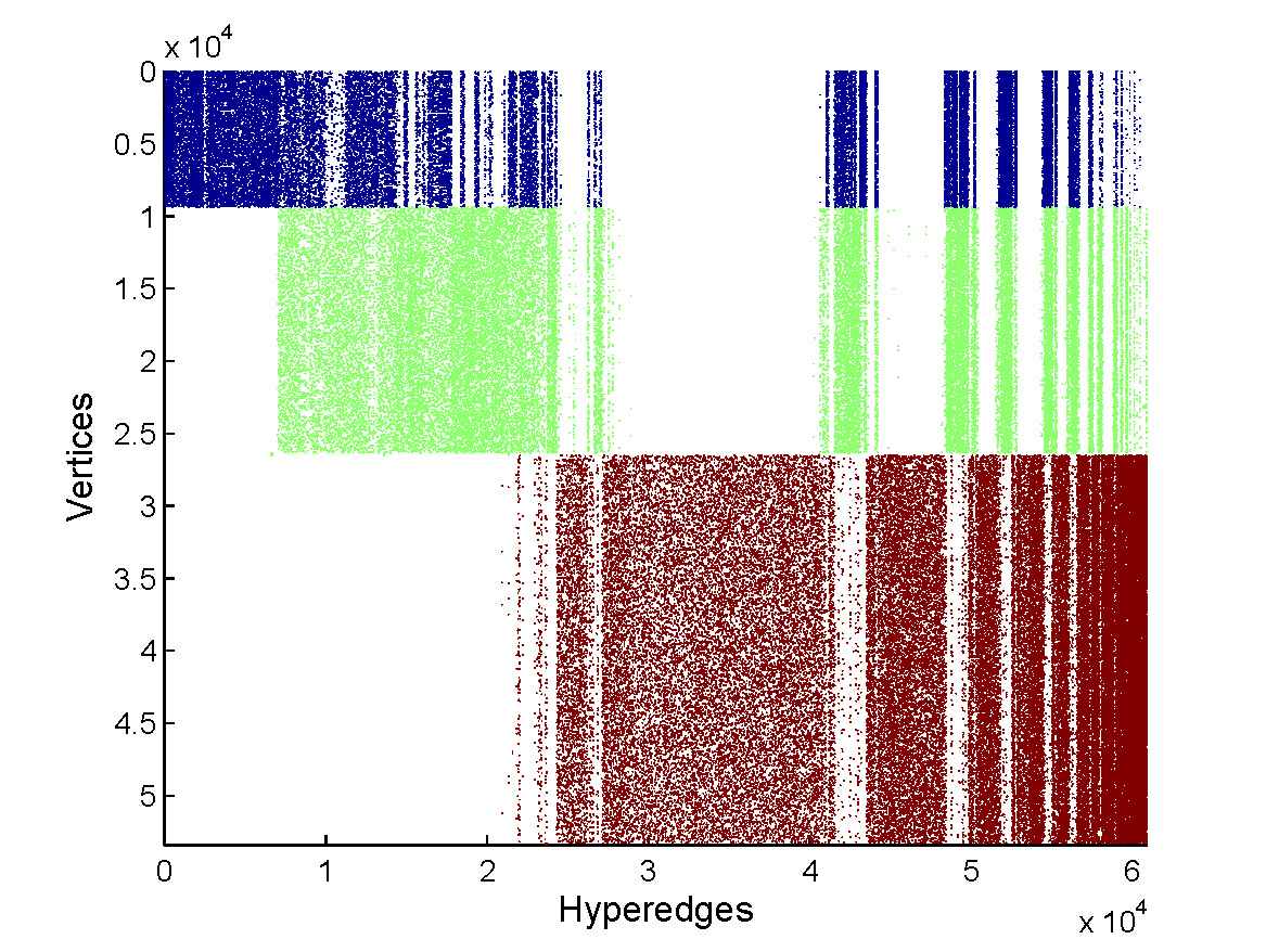
(a) Spectral approach

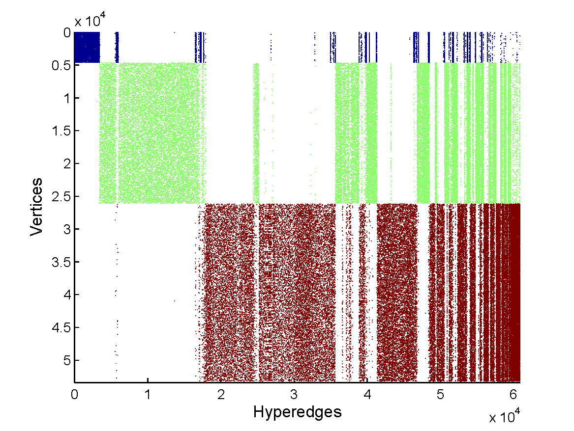
(b) RNHC

Figure 1: Clustering visualization on matrix ${\bf B}$ of ibm09. There are 3 clusters indicated by blue, green and red. Note that each column in the image represents a hyperedge. The number of colors of a column indicates the number of clusters that the corresponding hyperedge spans. It can be seen from Figure 1(a) that the blue and green clusters share many hyperedges (columns), which implies a bad clustering. And in Figure 1(b), less overlapping columns are produced by RNHC, which means a better clustering.

4.3 Accuracy Comparison

We evaluate the number of clusters from $2$ to $8$. For each trial, both algorithms will be tested for 40 times and the best NHC value will be picked for comparison. The reason why we compare the best NHC value instead of the average performance is that both algorithms utilize the K-Means algorithm for final clustering, whose result depends on the starting point. Sometimes K-Means simply fails to obtain $p$ clusters, which means that some of the clusters are empty. Moreover, K-Means occasionally produces extremely bad NHC values because of some bad starting point. Such failures may make the average performance meaningless. Furthermore, it is also hard to tell which trial fails and which one succeeds.

We test the objective value of NHC in (2) for each algorithm. The comparison of the objective value is shown in Figure 2. Note that a smaller objective value implies a better NHC. It can be seen that our algorithm produces a better objective value in most cases.

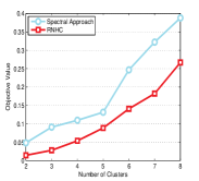
(a) ibm07

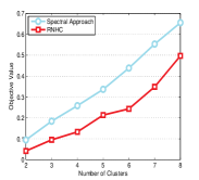
(b) ibm08

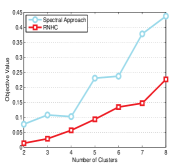
(c) ibm09

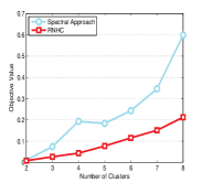
(d) ibm10

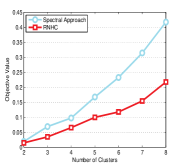
(e) ibm11

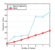
(f) ibm12

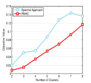
(g) ibm13

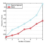
(h) ibm14

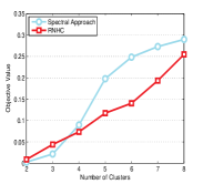
(i) ibm15

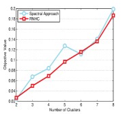
(j) ibm16

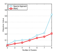
(k) ibm17

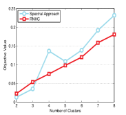
(l) ibm18

Figure 2: Objective value of clustering on ibm07-18

4.4 Speed Comparison

The comparison of the time for clustering on the largest 4 datasets is shown in Figure 3. To guarantee fairness, all the experiments are carried out in a single thread by setting “maxNumCompThreads(1)” in MATLAB. We can find that our RNHC algorithm is faster than the baseline in all cases.

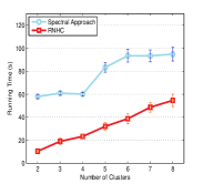
(a) ibm15

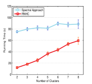
(b) ibm16

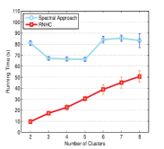
(c) ibm17

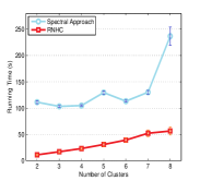
(d) ibm18

Figure 3: Running time of clustering on ibm15-18

5 Conclusion

In this paper we have proposed a new model to formulate the normalized hypergraph cut problem. Furthermore, we have provided an effective approach to relax the new model, and developed an efficient learning algorithm to solve the relaxed hypergraph cut problem. Experimental results on real hypergraphs have shown that our algorithm can outperform the state-of-the-art approach. It is interesting to apply our approach to other practical problems, such as the graph partitioning problem in distributed computation, in the future work.

References

- Agarwal et al. [2006] Sameer Agarwal, Kristin Branson, and Serge Belongie. Higher order learning with graphs. In Proceedings of the 23rd International Conference on Machine Learning, pages 17–24, 2006.
- Anandkumar et al. [2014] Animashree Anandkumar, Rong Ge, Daniel Hsu, and Sham M Kakade. A tensor approach to learning mixed membership community models. The Journal of Machine Learning Research, 15(1):2239–2312, 2014.
- Berge and Minieka [1973] Claude Berge and Edward Minieka. Graphs and hypergraphs, volume 7. North-Holland Publishing Company Amsterdam, 1973.
- Bolla [1993] Marianna Bolla. Spectra, euclidean representations and clusterings of hypergraphs. Discrete Mathematics, 117(1):19–39, 1993.
- Bulò and Pelillo [2009] Samuel R Bulò and Marcello Pelillo. A game-theoretic approach to hypergraph clustering. In Proceedings of Advances in Neural Information Processing Systems, pages 1571–1579, 2009.
- Catalyurek and Aykanat [1999] Umit V Catalyurek and Cevdet Aykanat. Hypergraph-partitioning-based decomposition for parallel sparse-matrix vector multiplication. IEEE Transactions on Parallel and Distributed Systems, 10(7):673–693, 1999.
- Chen et al. [2015] Rong Chen, Jiaxin Shi, Yanzhe Chen, and Haibo Chen. Powerlyra: Differentiated graph computation and partitioning on skewed graphs. In Proceedings of the 10th European Conference on Computer Systems, 2015.
- Cooper and Dutle [2012] Joshua Cooper and Aaron Dutle. Spectra of uniform hypergraphs. Linear Algebra and its Applications, 436(9):3268–3292, 2012.
- Ding and Yilmaz [2008] Lei Ding and Alper Yilmaz. Image segmentation as learning on hypergraphs. In Proceedings of the Seventh International Conference on Machine Learning and Applications, pages 247–252, 2008.
- Edelman et al. [1998] Alan Edelman, Tomás A Arias, and Steven T Smith. The geometry of algorithms with orthogonality constraints. SIAM Journal on Matrix Analysis and Applications, 20(2):303–353, 1998.
- Frieze and Kannan [2008] Alan M Frieze and Ravi Kannan. A new approach to the planted clique problem. In Proceedings of IARCS Annual Conference on Foundations of Software Technology and Theoretical Computer Science, volume 2, pages 187–198, 2008.
- Gonzalez et al. [2012] Joseph E Gonzalez, Yucheng Low, Haijie Gu, Danny Bickson, and Carlos Guestrin. Powergraph: Distributed graph-parallel computation on natural graphs. In Proceedings of the 10th USENIX Symposium on Operating Systems Design and Implementation, pages 17–30, 2012.
- Hagen and Kahng [1992] Lars Hagen and Andrew B Kahng. New spectral methods for ratio cut partitioning and clustering. IEEE Transactions on Computer-Aided Design of Integrated Circuits and Systems, 11(9):1074–1085, 1992.
- Jain et al. [2013] Nilesh Jain, Guangdeng Liao, and Theodore L Willke. Graphbuilder: scalable graph etl framework. In Proceedings of the First International Workshop on Graph Data Management Experiences and Systems, 2013.
- Karypis et al. [1999] George Karypis, Rajat Aggarwal, Vipin Kumar, and Shashi Shekhar. Multilevel hypergraph partitioning: applications in vlsi domain. IEEE Transactions on Very Large Scale Integration Systems,, 7(1):69–79, 1999.
- Li and Schuurmans [2011] Wenye Li and Dale Schuurmans. Modular community detection in networks. In Proceedings of the 22nd International Joint Conference on Artificial Intelligence, pages 1366–1371, 2011.
- Ng et al. [2001] Andrew Y Ng, Michael I Jordan, and Yair Weiss. On spectral clustering: Analysis and an algorithm. Proceedings of Advances in Neural Information Processing Systems, pages 849–856, 2001.
- Pu and Faltings [2012] Li Pu and Boi Faltings. Hypergraph learning with hyperedge expansion. In Proceedings of the European Conference on Machine Learning and Knowledge Discovery in Databases, pages 410–425. 2012.
- Rodríguez [2009] JA Rodríguez. Laplacian eigenvalues and partition problems in hypergraphs. Applied Mathematics Letters, 22(6):916–921, 2009.
- Shi and Malik [2000] Jianbo Shi and Jitendra Malik. Normalized cuts and image segmentation. IEEE Trans. Pattern Anal. Mach. Intell., 22(8):888–905, 2000.
- Tang and Liu [2010] Lei Tang and Huan Liu. Community Detection and Mining in Social Media. Synthesis Lectures on Data Mining and Knowledge Discovery. Morgan & Claypool Publishers, 2010.
- Trifunovic and Knottenbelt [2004] Aleksandar Trifunovic and William J Knottenbelt. Parkway 2.0: A parallel multilevel hypergraph partitioning tool. In Computer and Information Sciences-ISCIS 2004, pages 789–800. 2004.
- Wen and Yin [2013] Zaiwen Wen and Wotao Yin. A feasible method for optimization with orthogonality constraints. Mathematical Programming, 142(1-2):397–434, 2013.
- Wu and Leahy [1993] Zhenyu Wu and Richard M. Leahy. An optimal graph theoretic approach to data clustering: Theory and its application to image segmentation. IEEE Trans. Pattern Anal. Mach. Intell., 15(11):1101–1113, 1993.
- Xie et al. [2014] Cong Xie, Ling Yan, Wu-Jun Li, and Zhihua Zhang. Distributed power-law graph computing: Theoretical and empirical analysis. In Proceedings of Advances in Neural Information Processing Systems, pages 1673–1681, 2014.
- Zhou et al. [2006] Dengyong Zhou, Jiayuan Huang, and Bernhard Schölkopf. Learning with hypergraphs: Clustering, classification, and embedding. In Proceedings of Advances in Neural Information Processing Systems, pages 1601–1608, 2006.