Virtually Abelian Quantum Walks

Abstract

We study discrete-time quantum walks on Cayley graphs of non-Abelian groups, focusing on the easiest case of virtually Abelian groups. We present a technique to reduce the quantum walk to an equivalent one on an Abelian group with coin system having larger dimension. This method allows one to extend the notion of wave-vector to the virtually Abelian case and study analytically the walk dynamics. We apply the technique in the case of two quantum walks on virtually Abelian groups with planar Cayley graphs, finding the exact solution in terms of dispersion relation.

I Introduction

Discrete-time quantum walks (QWs) Ambainis et al. (2001); Aharonov et al. (2001); Knight et al. (2004) describe the unitary evolution of a quantum ``particle'' on a graph. Every node of the graph corresponds to a finite dimensional Hilbert space—the so-called coin system, representing the internal degree of freedom of the particle. The graph edges, on the other hand, represent local interactions among neighbouring sites.

Under the hypothesis of locality and homogeneity of the evolution one can show D'Ariano and Perinotti (2014) that the graph is the Cayley graph of a group. This allows one to use group representation theory to analyze the dynamics of the particle described by the walk. Classical random walks on Cayley graphs were studied as an integral part of discrete group theory Gromov , and only later developed as models of computation e.g. in Ref. Arrighi et al. (2012). The first paper addressing the issue of constructing QWs on Cayley graphs is Ref. Acevedo and Gobron (2006), where the focus is on Cayley graphs of free Abelian groups $\mathbb{Z}^{d}$. A first analysis investigating QWs on non-Abelian groups can be found in Ref. Acevedo et al. (2008). Here the authors consider the special class of scalar QWs (the coin system has dimension one) and classify the walks on Cayley graphs of finite groups presented with two or three generators.

In the present paper we study QWs on Cayley graphs, focusing attention on those groups that can be embedded in a Euclidean manifold quasi-isometrically, i.e. without distorting the distance defined in terms of minimum arc length on the graph (see Section II). Geometrically, QWs on these groups are the most general QWs with a flat geometry. The class of Cayley graphs that are quasi-isometrically embeddable in a Euclidean manifold coincides with virtually Abelian groups—including Abelian groups as a special case—that are generally non-Abelian. A critical issue for QWs on such groups is that, differently from the continuous flat case, they cannot be simply represented in the wave-vector space via the Fourier transform, computing for example the walk dispersion relation. Here we bridge this gap, showing how to solve the dynamics for walks on virtually Abelian groups in terms of a wave-vector representation.

The proposed solution consists in a coarse-graining procedure for coined quantum walks. Tiling procedures for QWs were recently proposed in Refs. Portugal et al. (2015a, b), where they are exploited for the study of QW search algorithms. The coarse-graining technique that we introduce here allows us to reduce the walks on virtually Abelian groups to walks on Abelian groups with a larger coin system.

On technical grounds, the above result enables the application of the Fourier analysis technique, with the definition of plane-waves and the adoption of the wave-vector as an invariant of the dynamics. As regards the physical motivation for the present analysis, we remind that the theory of quantum walks on Abelian groups has been used in Refs. D'Ariano and Perinotti (2014); Bisio et al. (2015, 2016a) providing a mechanism for understanding the dynamics of free relativistic quantum fields. In the same perspective, the approach that is proposed in the present paper can provide a similar understanding of the origin of spin and charge degrees of freedom. If the original walk has a trivial coin, indeed, the coarse-grained representation evolves particles of a spinorial or vectorial field, thus carrying non-trivial internal degrees of freedom, as studied in Ref. Bisio et al. (2016b), where the one-dimensional Dirac walk is derived by coarse-graining of a walk with trivial coin on the Cayley graph of the infinite dihedral group.

The technique that we introduce reduces the mathematical description of the walk to a simpler one, without loss of any information, and in this respect it cannot be considered a renormalization technique, in the spirit of Kadanoff's proposal for the treatment of discrete systems on larger scales Kadanoff (1966). However, our approach can also suggest the basic step for implementing the algebraic procedure of Ref. Bény and Osborne (2015), where renormalization is described in terms of CP embedding of C*-algebras corresponding to the system observables at different scales.

II Cayley graphs

In this section we review the notion of the Cayley graph of a group, and that of quasi-isometries between metric spaces, which allows to characterize the class of Cayley graphs quasi-isometrically embeddable in Euclidean spaces.

We can always think of a group $G$ as generated by a set of its elements $S_{+}$ called generators. We will denote by $S=S_{+}\cup S_{-}$ the union of $S_{+}$ with the set of its inverses $S_{-}$. Using $S$ as an alphabet, we formally build up words $w$ that represent multiplication of generators, corresponding to the group element $[w]\in G$. Generally there exist different words $w$ such that $[w]=e\in G$ is the identity. A set of relators $R=\{w_{n}\}$ is a set of words with $[w_{n}]=e$ such that every word $w$ with $[w]=e$ is a juxtaposition of words in $R$. For every group $G$, a choice of a generating set $S_{+}$ and a relator set $R$ provides a presentation $G=\langle S_{+}|R\rangle$ of the group. Any presentation of $G$ completely specifies $G$, and has the following graphical representation.

Definition 1 (Cayley graph)

Given a group $G$ and a set $S_{+}$ of generators of the group, the Cayley graph $\Gamma(G,S_{+})$ is defined as the directed edge-colored graph having vertex set $G$, edge set $\{(x,xg);x\in G,g\in S_{+}\}$, and a color assigned to each generator $g\in S_{+}$.

In the above representation the relators of the group are closed paths over the graph.
In the left of Fig. 1 we see an example of Cayley graph for the finite dihedral group $G=D_{3}$ with presentation $D_{3}=\langle a,b|a^{2},b^{3},(ab)^{2}\rangle$. In the middle and right of Fig. 1 we show two examples of Cayley graphs for infinite groups: the Abelian $\mathbb{Z}^{2}=\langle a,b|aba^{-1}b^{-1}\rangle$ and the non-Abelian group $F=\langle a,b|a^{5},b^{5},(ab)^{2}\rangle$ (a special case of Fuchsian group).

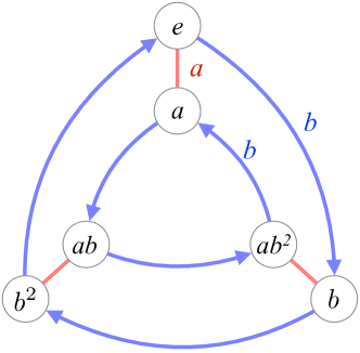
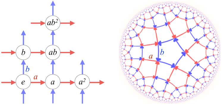
Figure 1: (colors online) Given a group $G$ and a set $S_{+}$ of generators, the Cayley graph $\Gamma(G,S_{+})$ is defined as the colored directed graph having set of nodes $G$, set of edges $\{(x,xh);x\in G,h\in S_{+}\}$, and a color assigned to each generator $h\in S_{+}$. Top: the Cayley graph of the dihedral group $D_{3}=\langle a,b|a^{2},b^{3},(ab)^{2}\rangle$. Bottom left: the Cayley graph of the Abelian group $\mathbb{Z}^{2}$ with presentation $\mathbb{Z}^{2}=\langle a,b|aba^{-1}b^{-1}\rangle$, where $a$ and $b$ are two commuting generators. Bottom right: the Cayley graph of the non-Abelian group $G=\langle a,b|a^{5},b^{5},(ab)^{2}\rangle$. The Abelian-group graph is embedded into the Euclidean space $\mathbb{R}^{2}$, the non-Abelian $G$ into the Hyperbolic space $\mathbb{H}_{2}$ with (negative) curvature.

Defining the length $l(w)$ of a word $w$ as the number of generators that compose it, one introduces the word-distance of two points $x_{1},x_{2}\in G$ as the length of the shortest word $w$ such that $[w]=x_{1}x_{2}^{-1}$. The Cayley graph equipped with the word-metric is a metric space. In the following section the Cayley graphs will be the lattice of a quantum walk.

Even for finitely presented groups (namely with $|S_{+}|$ and $|R|$ both finite), the algebraic properties of the group can be very hard to assess, or even provably undecidable (this is the case of triviality $G=\{e\}$, which is one of the Dehn problems Dehn (1911)). An effective way of studying the algebraic properties of groups is that of connecting them with the geometry of their Cayley graphs: this is the aim of geometric group theory de La Harpe (2000). The main idea of the approach is the notion of quasi-isometry due to Gromov Gromov (1984), which is defined as follows. Given two metric spaces $(M_{1},d_{1})$, $(M_{2},d_{2})$, we say that $M_{1}$ is quasi-isometric to $M_{2}$ if there is a map $f:M_{1}\to M_{2}$ such that there exist three constants $a>1$, $b>0$, $c>0$, such that $\forall x,y\in M_{1}$ one has

$$\frac{1}{a}d_{2}[f(x),f(y)]-b\leq d_{1}(x,y)\leq ad_{2}[f(x),f(y)]+b,$$

and $\forall z\in M_{2}$, there exists $x\in M_{1}$ such that

$$d_{2}[z,f(x)]\leq c.$$

The quasi-isometry is an equivalence relation between metric spaces Campbell (1999). For example, all Cayley graphs of a group $G$ are quasi-isometric Campbell (1999), and we will transfer the quasi-isometric class to $G$ itself. Moreover, quasi-isometric groups share relevant algebraic features. For example a group $G$ is quasi-isometric to a Euclidean space $\mathbb{R}^{n}$ if and only if it is virtually Abelian Kapovich (2012); de Cornulier et al. (2007), namely it has an Abelian subgroup $H$ with finite index (the number of cosets). In such a case $H\subseteq G$ is isomorphic to $\mathbb{Z}^{n}$ with $n\geq 0$. Two examples of virtually Abelian groups are considered in detail in Sections IV.1 and IV.2 (see also Figs. 2 and 3). Therefore, if $G$ is not virtually Abelian and embeddable in a metric manifold, then the manifold must have a nonvanishing curvature. An example is provided in the right of Fig. 1.

III Quantum walks on Cayley graphs

A quantum walk with $s$-dimensional coin system ($s\geq 1$) is a unitary evolution of a system with Hilbert space $\ell^{2}(V)\otimes\mathbb{C}^{s}$ such that

$$|\psi_{x,t+1}\rangle=\sum_{y\in V}A_{x,y}|\psi_{y,t}\rangle,$$

where $V\subseteq\mathbb{Z}$ and $A_{x,y}\in M_{s}(\mathbb{C})$ for $x,y\in V$ are $s\times s$ transition matrices. The set of nonnull matrices $A_{x,y}$ define a set $E\subseteq V\times V$ which can be regarded as the edge set of a graph $\Gamma(V,E)$. As we will see in the following, the conditions for the evolution to be unitary correspond to nontrivial constraints for the set of transition matrices. The case of interest in the present paper is when the graph is the Cayley graph $\Gamma(G,S_{+})$ of a group $G$, where the elements of $G$ are in bijective correspondence with the graph vertices $x\in V$. In addition the different colors and orientations of the edges from $x\in V$ correspond to different transition matrices $\{A_{g}\}_{g\in S}$ (meaning that $\forall x\,A_{x,xg}=A_{g}$). The independence of the matrix set of $x\in G$ corresponds to the homogeneity of the walk, whereas the finiteness of the set $S$ is the assumption of locality D'Ariano and Perinotti (2014).

If we now consider the right regular representation $T_{g}$ of the finitely generated group $G$, acting on $\ell^{2}(G)$ as $T_{g}|x\rangle:=|xg^{-1}\rangle$, we can write the quantum walk as

$$A:=\sum_{g\in S}T_{g}\otimes A_{g}.$$ (1)

The unitarity conditions for the walk operator (1) are $AA^{\dagger}=A^{\dagger}A=T_{e}\otimes I_{s}$ which imply

$$\sum\limits_{gg^{\prime-1}=f}A_{g}A_{g^{\prime}}^{\dagger} =\sum\limits_{g^{-1}g^{\prime}=f}A_{g}^{\dagger}A_{g^{\prime}}=0,\ \ \ \text{(with $f\neq e$)},$$ (2)

$$\sum\limits_{g\in S}A_{g}A_{g}^{\dagger} =\sum\limits_{g\in S}A_{g}^{\dagger}A_{g}=I_{s},$$ (3)

where $I_{s}$ is the identity operator over $\mathbb{C}^{s}$. Another relevant symmetry of a QW on a Cayley graph is the isotropy, saying that ``any direction on $\Gamma(G,S_{+})$ is equivalent''. This condition is translated in mathematical terms requiring that there exists a subset $S^{\prime}$ of $S$, with $S_{+}\subseteq S^{\prime}$, and a unitary representation $U$ over $\mathbb{C}^{s}$ of a group $Q$ of graph automorphisms, transitive over $S^{\prime}$, such that one has the covariance condition

$$A=\sum_{g\in S}T_{g}\otimes A_{g}=\sum_{g\in S}T_{f(g)}\otimes U_{f}A_{g}U^{\dagger}_{f},\quad\forall f\in Q.$$ (4)

As shown in D'Ariano and Perinotti (2014), QWs satisfying isotropy can be classified imposing the condition

$$\sum\limits_{g\in S}A_{g}=I_{s}$$ (5)

and then multiplying the resulting transition matrices by an arbitrary unitary matrix commuting with the representation $U$ of the automorphisms group.

III.1 Quantum walks on Cayley graphs of Abelian groups

The simplest case of quantum walks on Cayley graphs is when the group is free Abelian, i.e. $\mathbb{Z}^{d}$, since the walk can be easily diagonalized by a Fourier transform. We will label the elements $\mathbf{x}\in\mathbb{Z}^{d}$, using the usual additive notation for the group composition. The right regular representation of $\mathbb{Z}^{d}$ is expressed as follows

$$T_{\mathbf{y}}\left|\mathbf{x}\right>=\left|\mathbf{x}-\mathbf{y}\right>.$$

The representation is decomposed into irreducible representations, which are all one-dimensional, over which one diagonalizes $T_{\mathbf{y}}$ via Fourier in the wave-vector space as follows

$$\left|\mathbf{k}\right>\mathrel{\mathop{:}}=\frac{1}{\left(2\pi\right)^{\frac{d}{2}}}\sum\limits_{\mathbf{x}\in\mathbb{Z}^{d}}e^{-i\mathbf{k}\cdot\mathbf{x}}\left|\mathbf{x}\right>,$$

where $\mathbf{k}$ belongs to the first Brillouin zone $\mathcal{B}\subseteq\mathbb{R}^{d}$, which is the largest set that contains vectors $\mathbf{k}$ corresponding to inequivalent elements $\left|\mathbf{k}\right>$. The walk is written in the direct integral decomposition

$$A=\int_{\mathcal{B}}d\mathbf{k}\left|\mathbf{k}\right>\left<\mathbf{k}\right|\otimes A_{\mathbf{k}},\quad A_{\mathbf{k}}:=\sum_{\mathbf{h}\in S}e^{-i\mathbf{k}\cdot\mathbf{h}}A_{\mathbf{h}},$$

where $A_{\mathbf{k}}$ is unitary for every $\mathbf{k}\in\mathcal{B}$. Notice that the Brillouin zone depends on $S$, which in turn corresponds to a specific Cayley graph of $\mathbb{Z}^{d}$; e.g. for $\mathbb{Z}^{3}$ one has different Brillouin zones depending on the choice of presentation, which can correspond to the simple cubic lattice, or the body-centered cubic one, etc. (for details, see Ref. D'Ariano and Perinotti (2014)).
Diagonalizing $A_{\mathbf{k}}$, one obtains

$$A_{\mathbf{k}}\left|u_{r}(\mathbf{k})\right>=e^{i\omega_{r}(\mathbf{k})}\left|u_{r}(\mathbf{k})\right>,$$

where the $\omega_{r}(\mathbf{k})$ are the dispersion relation of the walk, and $\left|u_{r}(\mathbf{k})\right>$ the corresponding eigenstates. The dispersion relation gives the kinematics of the walk, with its first and second derivatives providing respectively the group velocity and the diffusion coefficient of particle states.

While for free Abelian groups the Fourier transform approach is straightforward, this is no longer true for generally non-Abelian groups. However, for virtually Abelian groups the procedure is still possible as we will see in the next section.

IV Virtually Abelian quantum walks

In this section we study quantum walks on Cayley graphs of a virtually Abelian group $G$ with finite-index Abelian subgroup $H\cong\mathbb{Z}^{d}$ (this choice is not restrictive by the classification of Abelian groups). We will see how the virtual Abelianity of the group allows one to define a coarse-graining of the Cayley graph that leads to an equivalent quantum walk on a Cayley graph of $H$. The basic idea is to partition $G$ into cosets of $H$, denoting them by a finite set of labels. In the following we will consider right cosets without loss of generality. The vertices of the Cayley graph of $G$ are thus grouped into clusters—containing one vertex from each coset—that become the nodes of a new coarse-grained graph and are in correspondence with the elements of $H$. Correspondingly, one can find an equivalent walk in terms of the generators of $H$, designating the coset labels as additional internal degrees of freedom.

Firstly we will provide a formal definition of the intuitive notion of ``regular tiling of a Cayley graph''.

Definition 2 (Regular tiling)

Let $G$ be a virtually Abelian group and let $H$ be an Abelian subgroup of $G$ of finite index. If $G$ is finitely generated and $H\cong\mathbb{Z}^{d}$, we call regular tiling of order $l$ the following right cosets partition for the Cayley graph of $G$

$$\bigcup\limits_{j=1}^{l}Hc_{j}=G\qquad\text{(with $c_{1}=e$)}.$$

Notice that the regular tiling is not unique and depends on the choice of $H$ and that of the representatives $c_{j}$. For any choice we can now provide a wave-vector representation of the quantum walk.

Consider the quantum walk $A$ on the Cayley graph given by the following presentation

$$G:=\langle S_{+}|R\rangle=\langle g_{1},\ldots g_{n}|r_{1},\ldots,r_{m}\rangle,$$ (6)

$$A:=\sum_{g\in S}T_{g}\otimes A_{g},\quad\left(A:\ell^{2}(G)\otimes\mathbb{C}^{s}\rightarrow\ell^{2}(G)\otimes\mathbb{C}^{s}\right).$$

Consider a regular tiling for $G$ corresponding to an Abelian subgroup $H$ of index $l$ and right cosets representatives $c_{1},\ldots,c_{l}$. We show how the virtually Abelian quantum walk (6) on $\ell^{2}(G)\otimes\mathbb{C}^{s}$ can be regarded as an Abelian QW on $\ell^{2}(H)\otimes\mathbb{C}^{sl}$.

In the following we will adopt the vector notation for the elements of $H$, keeping the multiplicative notation for the general group composition in $G$. While this choice may be slightly confusing, it is unavoidable to define the Fourier transform. The notation $\mathbf{x}c_{j}$ should thus not be interpreted as the rescaling of the vector $\mathbf{x}$ by a scalar, but just as group composition in $G$.

From the disjointness of the cosets it follows that every $x\in G$ admits the unique decomposition $x=\mathbf{x}c_{j}$ with $\mathbf{x}\in H$. One can then define a unitary mapping between $\ell^{2}\left(G\right)$ and $\ell^{2}\left(H\right)\otimes\mathbb{C}^{l}$ as follows

$$U_{H}:\ell^{2}\left(G\right) \longrightarrow\ell^{2}\left(H\right)\otimes\mathbb{C}^{l},\qquad U_{H}\left|\mathbf{x}c_{j}\right>=\left|\mathbf{x}\right>\left|j\right>.$$

Now we can define the plane waves on cosets

$$\left|\mathbf{k}\right>_{j}\mathrel{\mathop{:}}=\frac{1}{\left(2\pi\right)^{\frac{d}{2}}}\sum\limits_{\mathbf{x}\in H}e^{-i\mathbf{k}\cdot\mathbf{x}}\left|\mathbf{x}c_{j}\right>,$$

which via the map $U_{H}$ define the vector $\left|\mathbf{k}\right>_{H}$ as follows

$$\begin{split}U_{H}\left|\mathbf{k}\right>_{j}&=\left|\mathbf{k}\right>_{H}\left|j\right>.\end{split}$$

One has that $\forall g\in S$, $\forall\mathbf{x}\in H$ and $\forall c_{j}$ there exist an element $\mathbf{x^{\prime}}\in H$ and a coset representative $c_{j^{\prime}}$ (with $j^{\prime}$ function of $\left(g,j\right)$) such that

$$\mathbf{x}c_{j}g^{-1}=:\mathbf{x}^{\prime}c_{j^{\prime}\left(g,j\right)},\qquad\mathbf{h}_{j,g}\mathrel{\mathop{:}}=\mathbf{x}-{\mathbf{x}^{\prime}}=c_{j^{\prime}\left(g,j\right)}gc_{j}^{-1}\in H.$$

Thus one has that the translation operator $T_{g}$ for an arbitrary generator $g\in S$ of $G$ acts on the coset plane waves as

$$\begin{split}T_{g}\left|\mathbf{k}\right>_{j}&=\frac{1}{\left(2\pi\right)^{\frac{d}{2}}}\sum\limits_{\mathbf{x}\in H}e^{-i\mathbf{k}\cdot\mathbf{x}}\left|\mathbf{x}c_{j}g^{-1}\right>=\\ &=\frac{1}{\left(2\pi\right)^{\frac{d}{2}}}\sum\limits_{\mathbf{x}^{\prime}\in H}e^{-i\mathbf{k}\cdot\left(\mathbf{h}_{j,g}+\mathbf{x}^{\prime}\right)}\left|\mathbf{x}^{\prime}c_{j^{\prime}\left(g,j\right)}\right>=\\ &=e^{-i\mathbf{k}\cdot\mathbf{h}_{j,g}}\left|\mathbf{k}\right>_{j^{\prime}\left(g,j\right)},\end{split}$$ (7)

and on the wave-vector $\left|\mathbf{k}\right>_{H}\left|j\right>$ as

$$\begin{split}\left(U_{H}T_{g}U_{H}^{\dagger}\right)\left|\mathbf{k}\right>_{H}\left|j\right>&=e^{-i\mathbf{k}\cdot\mathbf{h}_{j,g}}\left|\mathbf{k}\right>_{H}\left|j^{\prime}\left(g,j\right)\right>.\end{split}$$ (8)

The last equation shows that $\left|\mathbf{k}\right>_{H}$ is an invariant space of the coarse-grained generators

$$\tilde{T}_{g}\mathrel{\mathop{:}}=U_{H}T_{g}U_{H}^{\dagger}\quad(\tilde{T}_{g}:\ell^{2}(H)\otimes\mathbb{C}^{l}\rightarrow\ell^{2}(H)\otimes\mathbb{C}^{l}).$$ (9)

While $T_{g}$ in the original walk description was changing the coset wave-vector (see Eq. (7)), its coarse-grained version $\tilde{T}_{g}$ keeps the wave-vector $\left|\mathbf{k}\right>_{H}$ invariant (up to a phase factor dependent on the generator $g$) with a non trivial action only on the additional coin system $\mathbb{C}^{l}$ (see Eq. (8)).

Accordingly, this mapping allows to diagonalize the generators of $G$ over the wave-vector space of $\ell^{2}(H)\otimes\mathbb{C}^{l}$ exploiting their action on the additional degrees of freedom. The coarse-grained quantum walk is thus given by

$$\mathcal{R}\left[A\right]\mathrel{\mathop{:}}=\left(U_{H}\otimes I\right)A\left(U_{H}\otimes I\right)^{\dagger}=\sum\limits_{g}\tilde{T}_{g}\otimes A_{g}.$$

Now, evaluating the matrix elements for the translations $\tilde{T}_{g}$, with $g\in S$

$$\left<\mathbf{k}\right|_{H}\left<i\right|\tilde{T}_{g}\left|\mathbf{k}\right>_{H}\left|j\right>=e^{-i\mathbf{k}\cdot\mathbf{h}_{j,g}}\delta_{i,j^{\prime}\left(g,j\right)},\quad i,j=1,\dots,l,$$

we can finally obtain the wave-vector representation of the walk $A_{\mathbf{k}}$. The last one is block-partitioned with block $ij$ given by

$$(A_{\mathbf{k}})_{ij}=\sum_{g:j^{\prime}(g,j)=i}A_{g}e^{-i\mathbf{k}\cdot\mathbf{h}_{j,g}}.$$

Notice that coarse-grained QWs corresponding to different choices of the regular tiling are unitarily equivalent. Let $U_{H},V_{H^{\prime}}$ be the coarse-graining unitary operators corresponding to two different choices of the subgroup of finite index (or even just to two different choices of the coset representatives for the same subgroup $H=H^{\prime}$): then, defining $\mathcal{R}\left[A\right]\mathrel{\mathop{:}}=\left(U_{H}\otimes I\right)A\left(U_{H}\otimes I\right)^{\dagger}$ and $\mathcal{R}^{\prime}\left[A\right]\mathrel{\mathop{:}}=\left(V_{H^{\prime}}\otimes I\right)A\left(V_{H^{\prime}}\otimes I\right)^{\dagger}$, one has that the two coarse-grained QWs are connected through the unitary mapping

$$\mathcal{R}^{\prime}\left[A\right]=\left(V_{H^{\prime}}U_{H}^{\dagger}\otimes I\right)\mathcal{R}\left[A\right]\left(V_{H^{\prime}}U_{H}^{\dagger}\otimes I\right)^{\dagger}.$$

In particular, two different choices do not change the dispersion relation.

While we defined the coarse-graining of a QW restricting to the case of interest of virtually Abelian groups, the procedure is general and can be easily defined for QWs on any arbitrary group $G$ which is virtually $G^{\prime}$ (namely any $G$ having a non-Abelian subgroup $G^{\prime}$ of finite index $l^{\prime}$). Indeed, also in this case the procedure can be performed as described above through a unitary mapping $U_{G^{\prime}}$ between $\ell^{2}\left(G\right)$ and $\ell^{2}\left(G^{\prime}\right)\otimes\mathbb{C}^{l^{\prime}}$, leading to a QW on a Cayley graph of $G^{\prime}$ with a larger coin system. However, one is not able to define plane waves on the cosets of $G^{\prime}$ if this is not Abelian, and this does not allow one to represent the walk in the k-space.

In the following we present the first two examples of QWs on non-Abelian groups whose evolution is analytically solved via the procedure described in this section.

IV.1 Example of a massive virtually Abelian QW

Let us consider the virtually Abelian group $G_{1}$ with the presentation

$$G_{1}=\langle a,b\ |\ a^{4},b^{4},(ab)^{2}\rangle,$$

and with Cayley graph corresponding to the simple square lattice, modulo a suitable re-coloring and re-orienting of the edges (see Fig. 2).

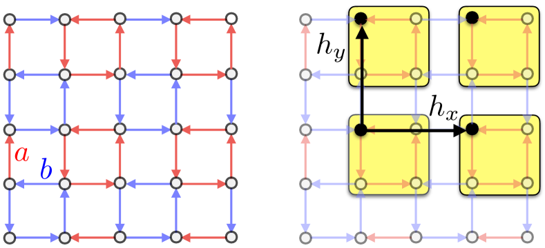
Figure 2: (colors online) Left: the Cayley graph of $G_{1}$ corresponding to the presentation $G_{1}=\langle a,b\ |\ a^{4},b^{4},{\left(ab\right)}^{2}\rangle$. The group is clearly not Abelian ($a$ and $b$ do not commute) but it is virtually Abelian. Right: a possible regular tiling of the Cayley graph of $G_{1}$. First we choose a subgroup (subgraph) isomorphic to $\mathbb{Z}^{2}$, in the figure the black sites given by the subgroup generators $h_{x}=a^{-1}b$ and $h_{y}=ba^{-1}$, which commute. The subgroup has index four and we choose a set of cosets representatives, in the figure $e,a,a^{2},a^{3}$, which define the tiling, each tile containing four elements of $G_{1}$.

Solving the unitarity constraints for

$$A=\sum_{g\in\{a,b,a^{-1},b^{-1}\}}T_{g}\otimes A_{g}$$

on the Hilbert space $\ell^{2}(G_{1})\otimes\mathbb{C}^{s}$ we obtain the admissible QWs on the Cayley graph of $G_{1}$ and with two-dimensional coin system. Due to the relators of the $G_{1}$ the first unitary condition (2) leads to the following relations

$$\begin{split}&A_{i^{-1}}A_{{j}^{-1}}^{\dagger}=A_{i^{-1}}^{\dagger}A_{{j}^{-1}}=\\ &=A_{i}A_{{j}}^{\dagger}=A_{i}^{\dagger}{A_{{j}}}=0,\qquad i\neq j\in\{a,b\}\end{split}$$ (10)

$$\begin{split}&A_{i}A_{j^{-1}}^{\dagger}+A_{{j}^{-1}}A_{i}^{\dagger}=\\ &=A_{i^{-1}}^{\dagger}A_{j}+A_{j}^{\dagger}A_{{i}^{-1}}=0,\qquad i,j\in\{a,b\},\end{split}$$ (11)

while the constraint (3) gives

$$\begin{split}&A_{a}A^{\dagger}_{a}+A_{b}A^{\dagger}_{b}+A_{a^{-1}}A^{\dagger}_{a^{-1}}+A_{b^{-1}}A^{\dagger}_{b^{-1}}=\\ &=A^{\dagger}_{a}A_{a}+A^{\dagger}_{b}A_{b}+A^{\dagger}_{a^{-1}}A_{a^{-1}}+A^{\dagger}_{b^{-1}}A_{b^{-1}}=I_{s}.\end{split}$$ (12)

From Eqs. (LABEL:eq:ort1) one can see that for $s=1$ at least one of the transition matrices must be null, contradicting the hypothesis (the edges of the graph correspond to non null transition matrices) hence there is no quantum walk on the considered Cayley graph. The simplest case is thus $s=2$, and in Appendix A we show that assuming the isotropy of the QW (see Section III) the solutions are divided into two non-unitarily equivalent classes

$$A^{\mathrm{I}}_{a} =\zeta^{\pm}Z_{\pm}\begin{pmatrix}1&0\\ 0&0\end{pmatrix}, A^{\mathrm{I}}_{b} =\zeta^{\pm}Z_{\pm}\begin{pmatrix}0&0\\ 0&1\end{pmatrix},$$

$$A^{\mathrm{I}}_{a^{-1}} =(A^{\mathrm{I}}_{a})^{\dagger}, A^{\mathrm{I}}_{b^{-1}} =(A^{\mathrm{I}}_{b})^{\dagger},$$

$$A^{\mathrm{II}}_{a} =A^{\mathrm{I}}_{a}, A^{\mathrm{II}}_{b} =A^{\mathrm{I}}_{b}, A^{\mathrm{II}}_{a^{-1}} =(A^{I}_{b})^{\dagger}, A^{\mathrm{II}}_{b^{-1}} =(A^{\mathrm{I}}_{a})^{\dagger},$$

where $\zeta^{\pm}:=\frac{1\pm i}{2}$ and $Z_{\pm}:=nI_{2}\pm im\sigma_{x}$ with $n^{2}+m^{2}=1$, $n,m\geq 0$.

In order to solve this class of walks analytically we apply the algorithm of Section IV. First we choose an Abelian subgroup of finite index $H\cong\mathbb{Z}^{2}$, and this is the group generated by $\mathbf{h}_{x}=a^{-1}b$, $\mathbf{h}_{y}=ba^{-1}$ of index four. Then we chose the regular tiling of the Cayley graph of $G_{1}$ achieved by the coset partition

$$G_{1}=\bigcup_{j=0}^{3}Hc_{j},\quad c_{j}=a^{j}.$$

Now we can define the plane waves on the cosets

$$\left|\mathbf{k}\right>_{j}\mathrel{\mathop{:}}=\frac{1}{2\pi}\sum\limits_{\mathbf{x}\in H}e^{-i\mathbf{k}\cdot\mathbf{x}}\left|\mathbf{x}a^{j}\right>,\ \ j=0,1,2,3,$$

and compute the action of the original walk on the cosets wave-vectors

$$T_{a}\left|\mathbf{k}\right>_{0} =\left|\mathbf{k}\right>_{3}, T_{a}\left|\mathbf{k}\right>_{1} =\left|\mathbf{k}\right>_{0},$$

$$T_{a}\left|\mathbf{k}\right>_{2} =\left|\mathbf{k}\right>_{1}, T_{a}\left|\mathbf{k}\right>_{3} =\left|\mathbf{k}\right>_{2},$$

$$T_{b}\left|\mathbf{k}\right>_{0} =e^{-ik_{x}}\left|\mathbf{k}\right>_{3}, T_{b}\left|\mathbf{k}\right>_{1} =e^{-ik_{y}}\left|\mathbf{k}\right>_{0},$$

$$T_{b}\left|\mathbf{k}\right>_{2} =e^{ik_{x}}\left|\mathbf{k}\right>_{1}, T_{b}\left|\mathbf{k}\right>_{3} =e^{ik_{y}}\left|\mathbf{k}\right>_{2},$$

$$T_{a^{-1}}\left|\mathbf{k}\right>_{0} =\left|\mathbf{k}\right>_{1}, T_{a^{-1}}\left|\mathbf{k}\right>_{1} =\left|\mathbf{k}\right>_{2},$$

$$T_{a^{-1}}\left|\mathbf{k}\right>_{2} =\left|\mathbf{k}\right>_{3}, T_{a^{-1}}\left|\mathbf{k}\right>_{3} =\left|\mathbf{k}\right>_{0},$$

$$T_{b^{-1}}\left|\mathbf{k}\right>_{0} =e^{ik_{y}}\left|\mathbf{k}\right>_{1}, T_{b^{-1}}\left|\mathbf{k}\right>_{1} =e^{-ik_{x}}\left|\mathbf{k}\right>_{2},$$

$$T_{b^{-1}}\left|\mathbf{k}\right>_{2} =e^{-ik_{y}}\left|\mathbf{k}\right>_{3}, T_{b^{-1}}\left|\mathbf{k}\right>_{3} =e^{ik_{x}}\left|\mathbf{k}\right>_{0},$$

where $k_{x}=\mathbf{k}\cdot\mathbf{h}_{x},\ k_{y}=\mathbf{k}\cdot\mathbf{h}_{y}$. It follows the expression for the coarse-grained QW

$$\mathcal{R}\left[A\right] =\int_{\mathcal{A}}d\mathbf{k}\left|\mathbf{k}\right>\left<\mathbf{k}\right|_{H}\otimes\mathcal{R}\left[A\right]_{\mathbf{k}},$$

where

$$\begin{aligned} \mathcal{R}\left[A\right]_{\mathbf{k}}&=\begin{pmatrix}A_{k_{y}}&A_{k_{x}}^{{}^{\prime}}\\ A_{-k_{x}}^{{}^{\prime}}&A_{-k_{y}}\end{pmatrix}\\ A_{k}&=\begin{pmatrix}0&A_{a}+e^{-ik}A_{b}\\ A_{a^{-1}}+e^{ik}A_{b^{-1}}&0\end{pmatrix},\\ A_{k}^{{}^{\prime}}&=\begin{pmatrix}0&A_{a^{-1}}+e^{ik}A_{b^{-1}}\\ A_{a}+e^{-ik}A_{b}&0\end{pmatrix}.\end{aligned}$$

By diagonalizing the $8\times 8$ matrix $\mathcal{R}\left[A\right]_{\mathbf{k}}$ we can finally compute the four eigenvalues $e^{-i\omega^{\pm}_{r}(k_{x},k_{y})}$, $r=1,2$ (each with multiplicity 2) of the coarse-grained walk with

$$\omega^{\pm}_{1}=\pm\arccos\alpha(\nu,k_{1},k_{2})-\pi/4,\quad\omega_{2}=\omega_{1}^{\pm}-\pi,$$

$$\alpha(\nu,k_{1},k_{2}):=\nu\sqrt{\frac{1}{2}\left(\cos^{2}\frac{k_{x}}{2}+\cos^{2}\frac{k_{y}}{2}\right)},$$

and $\nu=n$ ( respectively $\nu=m$) for the first (respectively second) class of solutions. The $\omega_{r}$ provides the QW dispersion relations providing the information on the kinematics of particle states. Close to the minimum of the dispersion relation, namely for small wave-vectors, one recovers a massive relativistic dispersion relation, with mass given by $\sqrt{1-\nu^{2}}$. The mass is upper bounded by one and at the bound the dispersion relation becomes flat (this feature is due to unitarity and has already been pointed out in Refs. D'Ariano and Perinotti (2014); D'Ariano (2012); Bisio et al. (2015)). In this example we observe how the non-Abelianity of the group $G_{1}$ induces a ``massive'' non trivial dynamics for the coarse-grained QW on the Abelian group $H$.

IV.2 Example of a massless virtually Abelian QW

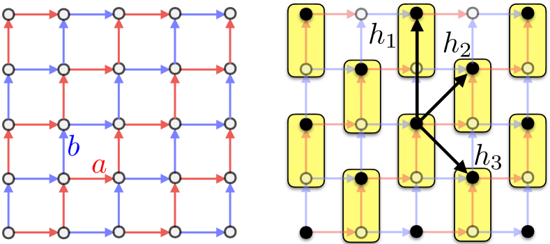
Figure 3: (colors online) Left: the Cayley graph of $G_{2}$ corresponding to the presentation $G_{2}=\langle a,b\ |\ a^{2}b^{-2}\rangle$. The group is not Abelian ($a$ and $b$ do not commute) but it is virtually Abelian. Right: a regular tiling of the Cayley graph of $G_{2}$. First we choose a subgroup (subgraph) isomorphic to $\mathbb{Z}^{2}$, in the figure the black sites gien by the subgroup commuting generators $h_{1}=ba$ and $h_{2}=a^{2}$. The subgroup has index two and we choose a set of cosets representatives, in the figure $e,a$, which define the tiling, each tile containing two elements of $G_{2}$.

In this section we consider another virtually Abelian group quasi-isometric to $\mathbb{R}^{2}$

$$G_{2}=\langle a,b\ |\ a^{2}b^{-2}\rangle,$$

whose Cayley graph is depicted in Fig. 3 and has vertices on the simple square lattice.

As in the previous section we start deriving the most general isotropic QW

$$A=\sum_{g\in\{a,b,a^{-1},b^{-1}\}}T_{g}\otimes A_{g}$$

on the Cayley graph of $G_{2}$ solving the unitarity constraints on the transition matrices. Using the relators of the group it is easy to see that the first unitary condition (2) leads to the following relations

$$A_{i}A_{{j}^{-1}}^{\dagger}=A_{i}^{\dagger}A_{{j}^{-1}}=0,$$ (13)

$$\begin{split}&A_{i}A_{j}^{\dagger}+A_{{i}^{-1}}A_{{j}^{-1}}^{\dagger}=A_{i}^{\dagger}{A_{j}}+A_{{i}^{-1}}^{\dagger}{A_{{j}^{-1}}}=\\ &=A_{i}A_{{i}^{-1}}^{\dagger}+A_{j}A_{{j}^{-1}}^{\dagger}=A_{i}^{\dagger}{A_{{i}^{-1}}}+A_{j}^{\dagger}{A_{{j}^{-1}}}=0,\end{split}$$ (14)

for $i\neq j\in\{a,b\}$, while the constraint (3) gives

$$\begin{split}&A_{a}A^{\dagger}_{a}+A_{b}A^{\dagger}_{b}+A_{a^{-1}}A^{\dagger}_{a^{-1}}+A_{b^{-1}}A^{\dagger}_{a^{-1}}=\\ &=A^{\dagger}_{a}A_{a}+A^{\dagger}_{b}A_{b}+A^{\dagger}_{a^{-1}}A_{a^{-1}}+A^{\dagger}_{b^{-1}}A_{b^{-1}}=I_{s}.\end{split}$$ (15)

As in the previous example there is no QW on the considered Cayley graph with $s=1$. In Appendix B we prove that for $s=2$ the only two solutions are

$$\begin{split}A^{\mathrm{I}}_{a}&=\frac{1}{2}\begin{pmatrix}1&0\\ 1&0\end{pmatrix},\quad A^{\mathrm{I}}_{b}=\frac{1}{2}\begin{pmatrix}1&0\\ -1&0\end{pmatrix},\\ A^{\mathrm{I}}_{a^{-1}}&=\frac{1}{2}\begin{pmatrix}0&1\\ 0&1\end{pmatrix},\quad A^{\mathrm{I}}_{b^{-1}}=\frac{1}{2}\begin{pmatrix}0&-1\\ 0&1\end{pmatrix},\end{split}$$

$$A_{g}^{\mathrm{II}} =Y{\left(A_{g}^{\mathrm{I}}\right)}^{t}Y^{\dagger},\ \ \ Y=\frac{1}{\sqrt{2}}\left(I_{2}+i\sigma_{y}\right),$$

which are anti-unitarily equivalent.

We choose now the Abelian subgroup $H\cong\mathbb{Z}^{2}$ of index $2$ generated by $\mathbf{h}_{2}=a^{2}$, $\mathbf{h}_{3}=a^{-1}b$ and the $G_{2}$ regular tiling partition

$$G_{2}=H\cup Hc,\ \ c=a^{-1}.$$

It is then useful to introduce the graph corresponding to the presentation

$$H=\langle\mathbf{h}_{1},\mathbf{h}_{2},\mathbf{h}_{3}\ |\ \mathbf{h}_{1}-\left(\mathbf{h}_{2}-\mathbf{h}_{3}\right)\rangle,$$ (16)

whose vertices are a subset of the vertices of the original Cayley graph of $G$ (the Abelian notation is used since $H\cong\mathbb{Z}^{2}$) where we added the redundant generator $\mathbf{h}_{1}=ba$.

Due to the normality (since it is of index 2) of $H$ in $G_{2}$ we can define the wave-vector on cosets, namely the invariant spaces under the $T_{\mathbf{h}_{i}}$, $i=1,2,3$,

$$\left|\mathbf{k}\right>_{0}\mathrel{\mathop{:}}=\frac{1}{2\pi}\sum\limits_{\mathbf{x}\in H}e^{-i\mathbf{k}\cdot\mathbf{x}}\left|\mathbf{x}\right>,\ \left|\mathbf{k}\right>_{1}\mathrel{\mathop{:}}=\frac{1}{2\pi}\sum\limits_{\mathbf{x}\in H}e^{-i\mathbf{k}\cdot\mathbf{x}}\left|\mathbf{x}a^{-1}\right>.$$

Evaluating the action of the generator of $G_{2}$ on the $\left|\mathbf{k}\right>_{j}$, one can reconstruct the coarse-grained walk $\mathcal{R}[A]$, which will be written in terms of the generators of $H$ and their inverses. First we evaluate the action of the $G_{2}$ generators on the cosets wave-vectors

$$T_{a}\left|\mathbf{k}\right>_{0} =\left|\mathbf{k}\right>_{1}, T_{a}\left|\mathbf{k}\right>_{1} =e^{-ik_{2}}\left|\mathbf{k}\right>_{0},$$

$$T_{b}\left|\mathbf{k}\right>_{0} =e^{-ik_{3}}\left|\mathbf{k}\right>_{1}, T_{b}\left|\mathbf{k}\right>_{1} =e^{-ik_{1}}\left|\mathbf{k}\right>_{0},$$

$$T_{a^{-1}}\left|\mathbf{k}\right>_{0} =e^{ik_{2}}\left|\mathbf{k}\right>_{1}, T_{a^{-1}}\left|\mathbf{k}\right>_{1} =\left|\mathbf{k}\right>_{0},$$

$$T_{b^{-1}}\left|\mathbf{k}\right>_{0} =e^{ik_{1}}\left|\mathbf{k}\right>_{1}, T_{b^{-1}}\left|\mathbf{k}\right>_{1} =e^{ik_{3}}\left|\mathbf{k}\right>_{0}.$$

It follows the off-diagonal expression for the renormalized walk

$$\mathcal{R}[A]_{\mathbf{k}} =\begin{pmatrix}0&A_{\mathbf{k}}\\ A_{\mathbf{k}}^{\prime}&0\end{pmatrix},$$ (17)

$$A_{\mathbf{k}} =e^{-ik_{2}}A_{a}+e^{-ik_{1}}A_{b}+A_{a^{-1}}+e^{ik_{3}}A_{b^{-1}},$$

$$A_{\mathbf{k}}^{\prime} =A_{a}+e^{-ik_{3}}A_{b}+e^{ik_{2}}A_{a^{-1}}+e^{ik_{2}}A_{b^{-1}}.$$

Exploiting the relator in (16) equations (17) become

$$A_{\mathbf{k}}=e^{-i\frac{k_{y}}{2}}B_{\mathbf{k}},\qquad A_{\mathbf{k}}^{\prime}=e^{i\frac{k_{y}}{2}}\sigma_{z}B_{\mathbf{k}}\sigma_{z},$$

$$B_{\mathbf{k}}\mathrel{\mathop{:}}=\left(e^{-i\frac{k_{x}}{2}}A_{a}+e^{-i\frac{k_{y}}{2}}A_{b}+e^{i\frac{k_{y}}{2}}A_{a^{-1}}+e^{i\frac{k_{x}}{2}}A_{b^{-1}}\right),$$

where $k_{x}:=k_{2}+k_{3}$ and $k_{y}:=k_{1}$. Defining

$$V\mathrel{\mathop{:}}=\begin{pmatrix}I&0\\ 0&e^{i\frac{k_{y}}{2}}\sigma_{z}\end{pmatrix},\qquad R:=\frac{1}{\sqrt{2}}\begin{pmatrix}1&1\\ 1&-1\end{pmatrix},$$

one has

$$\mathcal{R}[A]_{\mathbf{k}}=V(R\otimes I)\left(\sigma_{z}\otimes B_{\mathbf{k}}\sigma_{z}\right)(R^{\dagger}\otimes I)V^{\dagger}.$$ (18)

Accordingly $\mathcal{R}\left[A\right]_{\mathbf{k}}$ is unitarily equivalent to $\sigma_{z}\otimes B_{\mathbf{k}}\sigma_{z}$ whose four eigenvalues $e^{-i\omega_{r}^{\pm}(k_{x},k_{y})}$, $r=1,2$ are expressed in terms of the walk dispersion relations

$$\omega^{\pm}_{1}:=\pm\arccos\alpha(k_{x},k_{y})+\pi/2,\qquad\omega^{\pm}_{2}:=\omega^{\pm}_{1}+\pi,$$

$$\alpha(k_{x},k_{y}):=\frac{1}{2}\left(\sin\frac{k_{x}}{2}+\sin\frac{k_{y}}{2}\right).$$

We notice that this dispersion relations are equivalent, up to shifts in wave-vectors, to the Weyl QW one. The Weyl QW (which is the unique isotropic QW for $s=2$ on the Cayley graph $\mathbb{Z}^{2}=\langle a,b|aba^{-1}b^{-1}\rangle$ D'Ariano and Perinotti (2014)). While the coarse-graining procedure for the example in Section IV.1 led to a class of walks with ``massive'' dispersion relation, in this case the dispersion relation close to its minimum (for wave-vectors close to $(\pi,\pi)$) is linear in $\mathbf{k}$. In this sense the non-Abelianity of the original graph does not induce relevant effects on the dynamics of the coarse-grained QW.

We conclude analyzing the relation between the coarse-graining of the two solutions obtained in this section, namely $\mathcal{R}[A^{\mathrm{I}}]_{\mathbf{k}}$ and $\mathcal{R}[A^{\mathrm{II}}]_{\mathbf{k}}$. Through a block diagonal change of basis matrix, we saw that $\mathcal{R}[A^{I}]_{\mathbf{k}}$ is unitarily equivalent to $\sigma_{z}\otimes B_{\mathbf{k}}\sigma_{z}$. In Since two solutions $A^{\mathrm{I}}$ and $A^{\mathrm{II}}$ are connected by a local anti-unitary transformation (see Appendix B), $\mathcal{R}[A^{II}]_{\mathbf{k}}$ is, by linearity, unitarily equivalent to $\sigma_{z}\otimes\sigma_{z}B^{T}_{\mathbf{k}}$, which is just $\mathcal{R}[A^{I}]^{\dagger}_{-\mathbf{k}}$ (up to a change of basis). This means that the two coarse-grained QWs are connected by $\mathsf{PT}$ symmetry, with parity and time-reversal maps given by $\mathsf{P}:\mathbf{k}\longmapsto-\mathbf{k}$ and $\mathsf{T}:A\ \longmapsto A^{\dagger}$.

V Conclusions

In this manuscript we considered quantum walks on Cayley graphs of non-Abelian groups, with emphasis on the case of virtually Abelian groups. We devised a coarse-graining technique to reduce the quantum walk to an equivalent one on an Abelian group with coin system of larger dimension. This method, based on the group structure of the graph, allows one to extend the notion of wave-vector as an invariant of the walk dynamics to the virtually Abelian case. Within this framework, virtually Abelian QWs can be diagonalized in terms of a dispersion relation, which carries relevant kinematic information.

We derived the class of QWs allowed on two special virtually Abelian groups with planar Cayley graphs. We then applied the coarse-graining technique to solve the aforementioned walks analytically. Interestingly, for one of the two groups the dynamics of the QW leads to a massive dispersion relation by virtue of the presence of nontrivial cyclic subgroups.

The coarse-graining technique represents a crucial step in the derivation of the complete set of quantum walks allowed on Cayley graphs that are quasi-isometric to $\mathbb{R}^{d}$.

Finally, our technique can also be exploited as an intermediate step in a general renormalization procedure, where besides coarse-graining one also needs to implement the disposal of information for the purpose of changing the relevant scale of description of the walk dynamics. For example, this can be accomplished by an algebraic approach to renormalization as illustrated in Ref. Bény and Osborne (2015).

Appendix A Derivation of the QW in Section IV.1

Here we derive the walk in Section IV.1 on the Cayley graph of $G_{1}=\langle a,b\ |\ a^{4},b^{4},{\left(ab\right)}^{2}\rangle$. Assuming the isotropy of the walk (see Section III), we show how to solve the unitarity constraints Eqs. (LABEL:eq:ort1,LABEL:eq:sum1,LABEL:eq:norm1) obtained from the above Cayley graph. We take the polar decomposition of the QW transition matrices $A_{g}=V_{g}P_{g}$ ($g\in S=\{a,b,a^{-1},b^{-1}\}$) and considering that $P_{q}=P_{q}^{\dagger}$, the conditions in Eq.(LABEL:eq:ort1) become

$$V_{i^{\pm 1}}P_{i^{\pm 1}}{P_{{j}^{\pm 1}}}{V_{{j}^{\pm 1}}}^{\dagger} =0,$$ (19)

$$P_{i^{\pm 1}}{V_{i^{\pm 1}}}^{\dagger}{V_{{j}^{\pm 1}}}{P_{{j}^{\pm 1}}} =0.$$ (20)

Being the $V$ matrices unitary, we need to have $P_{i^{\pm 1}}{P_{{j}^{\pm 1}}}=0$, and being both $P_{i}$ and $P_{j}$ nonnull (all transition matrices are nonnull by definition) they must be both rank one. Moreover, from (19) one has

$$P_{i^{\pm 1}}=\alpha_{i^{\pm 1}}\left|+_{i^{\pm 1}}\right>\left<+_{i^{\pm 1}}\right|,\ \ P_{j^{\pm 1}}=\alpha_{j^{\pm 1}}\left|-_{i^{\pm 1}}\right>\left<-_{i^{\pm 1}}\right|,$$

with $\alpha_{g}>0$ and $\left\{\left|+_{g}\right>,\left|-_{g}\right>\right\}$ orthonormal bases for $\mathbb{C}^{2}$. From equation (20) we get $\left<+_{i^{\pm 1}}\right|{V_{i^{\pm 1}}}^{\dagger}V_{{j}^{\pm 1}}\left|-_{i^{\pm 1}}\right>=0$ and, since ${V_{i^{\pm 1}}}^{\dagger}V_{{j}^{\pm 1}}$ is unitary, it must be diagonal on the basis $\left\{\left|+_{i^{\pm 1}}\right>,\left|-_{i^{\pm 1}}\right>\right\}$ (with entries corresponding to phases). The $V_{g}$ are not uniquely determined by the polar decomposition, since the $A_{g}$ are not full rank. In fact, if $A_{i^{\pm 1}}=V_{i^{\pm 1}}P_{i^{\pm 1}}$ holds for a $V_{i^{\pm 1}}$, there exists an infinite class of unitary matrices $V_{i^{\pm 1}}^{\prime}$ such that $A_{i^{\pm 1}}=V_{i^{\pm 1}}^{\prime}P_{i^{\pm 1}}$: all the unitary matrices

$$V_{i^{\pm 1}}^{\prime}=V_{i^{\pm 1}}\left(\left|+_{i^{\pm 1}}\right>\left<+_{i^{\pm 1}}\right|+e^{i\theta_{i^{\pm 1}}}\left|-_{i^{\pm 1}}\right>\left<-_{i^{\pm 1}}\right|\right)$$ (21)

give the same polar decomposition for $A_{i^{\pm 1}}$. The same freedom holds for $A_{{j}^{\pm 1}}$, $j\neq i$ and one can always fix it computing

$$\begin{split}{V_{i^{\pm 1}}^{\prime}}^{\dagger}V_{j^{\pm 1}}^{\prime}&=e^{i\theta_{j^{\pm 1}}}\left<+_{i^{\pm 1}}\right|{V_{i^{\pm 1}}}^{\dagger}V_{j^{\pm 1}}\left|+_{i^{\pm 1}}\right>\left|+_{i^{\pm 1}}\right>\left<+_{i^{\pm 1}}\right|\\ &+e^{-i\theta_{i^{\pm 1}}}\left<-_{i^{\pm 1}}\right|{V_{i^{\pm 1}}}^{\dagger}V_{{j}^{\pm 1}}\left|-_{i^{\pm 1}}\right>\left|-_{i^{\pm 1}}\right>\left<-_{i^{\pm 1}}\right|\end{split}$$

and posing $e^{i\theta_{j^{\pm 1}}}\left<+_{i^{\pm 1}}\right|{V_{i^{\pm 1}}}^{\dagger}V_{j^{\pm 1}}\left|+_{i^{\pm 1}}\right>=1$ and $e^{-i\theta_{i^{\pm 1}}}\left<-_{i^{\pm 1}}\right|{V_{i^{\pm 1}}}^{\dagger}V_{j^{\pm 1}}\left|-_{i^{\pm 1}}\right>=1$. Accordingly one has

$$V_{i^{\pm 1}}^{\prime\dagger}V_{{j}^{\pm 1}}^{\prime}=I\Longrightarrow\ V_{{j}^{\pm 1}}^{\prime}=V_{i^{\pm 1}}^{\prime}$$ (22)

that leads to the following structure for the transition matrices

$$A_{a}=\alpha_{a}V\left|+_{a}\right>\left<+_{a}\right|,A_{b}=\alpha_{b}V\left|-_{a}\right>\left<-_{a}\right|,$$ (23)

$$A_{a^{-1}}=\alpha_{a^{-1}}W\left|+_{a^{-1}}\right>\left<+_{a^{-1}}\right|,$$ (24)

$$A_{b^{-1}}=\alpha_{b^{-1}}W\left|-_{a^{-1}}\right>\left<-_{a^{-1}}\right|,$$ (25)

with $\alpha_{g}>0$ and $\{\left|+_{q}\right>,\left|-_{q}\right>\}$ orthonormal bases for $\mathbb{C}^{2}$.

Combining (LABEL:eq:ort1) and (LABEL:eq:sum1) one obtains

$$A_{i^{-1}}A_{i}^{\dagger}A_{j^{-1}}=0,\qquad A_{i}A_{i^{-1}}^{\dagger}A_{j}=0,$$

$$A_{j}A_{i^{-1}}^{\dagger}A_{i}=0,\qquad A_{j^{-1}}A_{i}^{\dagger}A_{i^{-1}}=0.$$

and using the expression (23) for the $A_{g}$ we get

$$\left<+_{a}\vphantom{+_{a^{-1}}}\right|\left.+_{a^{-1}}\vphantom{+_{a}}\right>\left<-_{a^{-1}}\right|W^{\dagger}V\left|+_{a}\right>=0,$$ (26)

$$\left<-_{a}\vphantom{-_{a^{-1}}}\right|\left.-_{a^{-1}}\vphantom{-_{a}}\right>\left<+_{a^{-1}}\right|W^{\dagger}V\left|-_{a}\right>=0,$$

$$\left<+_{a}\vphantom{-_{a^{-1}}}\right|\left.-_{a^{-1}}\vphantom{+_{a}}\right>\left<+_{a^{-1}}\right|W^{\dagger}V\left|+_{a}\right>=0,$$

$$\left<-_{a}\vphantom{+_{a^{-1}}}\right|\left.+_{a^{-1}}\vphantom{-_{a}}\right>\left<-_{a^{-1}}\right|W^{\dagger}V\left|-_{a}\right>=0.$$

Considering that $\left<+_{a}\vphantom{-_{a^{-1}}}\right|\left.-_{a^{-1}}\vphantom{+_{a}}\right>=0\Leftrightarrow\left|+_{a}\right>=\left|+_{a^{-1}}\right>\Leftrightarrow\left<-_{a}\vphantom{+_{a^{-1}}}\right|\left.+_{a^{-1}}\vphantom{-_{a}}\right>=0$ (up to phase factors that would not appear in the $A_{g}$), condition (26) can be satisfied only in two cases

1. $\begin{aligned} \left<+_{a^{-1}}\right|W^{\dagger}V\left|-_{a}\right>=\left<-_{a^{-1}}\right|W^{\dagger}V\left|+_{a}\right>=0,\\ \end{aligned}$

2. $\begin{aligned} \left<-_{a^{-1}}\right|W^{\dagger}V\left|-_{a}\right>=\left<+_{a^{-1}}\right|W^{\dagger}V\left|+_{a}\right>=0.\end{aligned}$

Let's note that just two of the matrix elements which appear in (32) can be zero: indeed, suppose by contradiction that this is not be the case, let's define $U$ any of the possible matrices which connect the two orthonormal bases found; thus $U^{\dagger}W^{\dagger}V$ would have at least three vanishing matrix elements, but this is absurd for it is unitary. Accordingly, the two cases are:

1. $\begin{aligned} A^{\mathrm{I}}_{a}&=\alpha_{a}\mu W\left|+\right>\left<+\right|&A^{\mathrm{I}}_{b}&=\alpha_{b}\nu W\left|-\right>\left<-\right|\\ A^{\mathrm{I}}_{a^{-1}}&=\alpha_{a^{-1}}W\left|+\right>\left<+\right|&A^{\mathrm{I}}_{b^{-1}}&=\alpha_{b^{-1}}W\left|-\right>\left<-\right|,\end{aligned}$

2. $\begin{aligned} A^{\mathrm{II}}_{a}&=\alpha_{a}\mu W\left|+\right>\left<+\right|&A^{\mathrm{II}}_{b}&=\alpha_{b}\nu W\left|-\right>\left<-\right|\\ A^{\mathrm{II}}_{a^{-1}}&=\alpha_{a^{-1}}W\left|-\right>\left<-\right|&A^{\mathrm{II}}_{b^{-1}}&=\alpha_{b^{-1}}W\left|+\right>\left<+\right|,\end{aligned}$

with $\mu,\nu$ phase factors and each of them can be equal either to $i$ or to $-i$. From the condition (5), $W$ is found simply substituting the $A_{g}$ and inverting the resulting relation, while from the normalization (LABEL:eq:norm1) one can find the $\alpha_{g}$. The transition matrices for the case I are

$$A^{\mathrm{I}}_{a} =\zeta^{\pm}\begin{pmatrix}1&0\\ 0&0\end{pmatrix}, A_{b} =\zeta^{\pm}\begin{pmatrix}0&0\\ 0&1\end{pmatrix},$$

$$A^{\mathrm{I}}_{a^{-1}} =\zeta^{\mp}\begin{pmatrix}1&0\\ 0&0\end{pmatrix}, A^{\mathrm{I}}_{b^{-1}} =\zeta^{\mp}\begin{pmatrix}0&0\\ 0&1\end{pmatrix}.$$

where $A^{\mathrm{I}}_{a^{-1}}=(A^{\mathrm{I}}_{a})^{\dagger}$, $A^{\mathrm{I}}_{b^{-1}}=(A^{\mathrm{I}}_{b})^{\dagger}$, $\zeta^{\pm}\mathrel{\mathop{:}}=\frac{1\pm i}{2}$, while the solutions II are the same up to the swap $a^{-1}\leftrightarrow b^{-1}$.

It is now simple to verify that the solutions derived in this section satisfy the isotropy constraint (4). Indeed for the group $G_{1}:=\langle a,b\ |\ a^{4},b^{4},{\left(ab\right)}^{2}\rangle$ the only transitive automorphism of $S_{+}=\{a,b\}$ is the swap $a\leftrightarrow b$ of the generators. It is easy to verify that this automorphism is represented by the unitary matrix $\sigma_{x}$.

Accordingly we see that by left multiplication of the transition matrices with a unitary matrix commuting with $\sigma_{x}$—whose general form is

$$Z_{\pm}=nI\pm im\sigma_{x},$$

for $n,m\geq 0$ and $n^{2}+m^{2}=1$—both the unitarity conditions and the isotropy of the QW are unchanged. This shows that whole class of isotropic QWs on $G_{1}$ is obtained by left multiplication of the above solutions by the matrix $Z_{\pm}=nI\pm im\sigma_{x}$.

Appendix B Derivation of the QW in Section IV.2

In this appendix we present the derivation of the walk in Section IV.2 on the Cayley graph of $G_{2}=\langle a,b\ |\ a^{2}b^{-2}\rangle$. We know that this corresponds to solve the unitarity conditions in Eqs. (13,LABEL:eq:sum2,LABEL:eq:norm2) for the walk transition matrices. The procedure is very similar to the case analysed in the previous section but for the convenience of the reader we detail the full derivation.

Taking a polar decomposition $A_{g}=V_{g}P_{g}$ for the transition matrices and noticing that $P_{g}=P_{g}^{\dagger}$, Eq. (13) becomes

$$V_{i}P_{i}{P_{{j}^{-1}}}{V_{{j}^{-1}}}^{\dagger} =0,$$ (27)

$$P_{i}{V_{i}}^{\dagger}{V_{{j}^{-1}}}{P_{{j}^{-1}}} =0,$$ (28)

for $i\neq j\in\{a,b\}$. Being the $V$ matrices unitary, we need to have $P_{i^{\pm 1}}{P_{{j}^{\pm 1}}}=0$, and being both $P_{i}$ and $P_{j^{-1}}$ nonnull (all transition matrices are nonnull by definition) they must be both rank one. Furthermore from (27) one can write

$$P_{i}=\alpha_{i}\left|+_{i}\right>\left<+_{i}\right|,\ \ P_{j^{-1}}=\alpha_{j^{-1}}\left|-_{i}\right>\left<-_{i}\right|$$

with $\alpha_{q}>0$ and $\left\{\left|+_{i}\right>,\left|-_{i}\right>\right\}$ orthonormal bases for $\mathbb{C}^{2}$.

From equations (28) one finds that $\left<+_{i}\right|{V_{i}}^{\dagger}V_{{j}^{-1}}\left|-_{i}\right>=0$ and, since ${V_{i}}^{\dagger}V_{{j}^{-1}}$ is unitary, it must be diagonal on the basis $\left\{\left|+_{i}\right>,\left|-_{i}\right>\right\}$ (with entries given by phase factors). The $V_{q}$ are not uniquely determined by the polar decomposition, since the $A_{q}$ are not full rank. In fact, if $A_{i}=V_{i}P_{i}$ holds for a $V_{i}$, there exists an infinite class of unitary matrices $V_{i}^{\prime}$ such that $A_{i}=V_{i}^{\prime}P_{i}$:

$$V_{i}^{\prime}=V_{i}\left(\left|+_{i}\right>\left<+_{i}\right|+e^{i\theta_{i}}\left|-_{i}\right>\left<-_{i}\right|\right)$$

are unitary and give the $A_{i}$ polar decomposition for. The same holds for $A_{{j}^{-1}}$ and one can always fix this arbitrariness computing

$${V_{i}^{\prime}}^{\dagger}V_{j^{-1}}^{\prime}= e^{i\theta_{j^{-1}}}\left<+_{i}\right|{V_{i}}^{\dagger}V_{j^{-1}}\left|+_{i}\right>\left|+_{i}\right>\left<+_{i}\right|+$$ (29)

$$e^{-i\theta_{i}}\left<-_{i}\right|{V_{i}}^{\dagger}V_{{j}^{-1}}\left|-_{i}\right>\left|-_{i}\right>\left<-_{i}\right|$$ (30)

and taking $e^{i\theta_{j^{-1}}}\left<+_{i}\right|{V_{i}}^{\dagger}V_{j^{-1}}\left|+_{i}\right>=1$ and $e^{-i\theta_{i}}\left<-_{i}\right|{V_{i}}^{\dagger}V_{j^{-1}}\left|-_{i}\right>=1$. It follows ${V_{i}^{\prime}}^{\dagger}V_{{j}^{-1}}^{\prime}=I_{2}\ \Longrightarrow\ V_{{j}^{-1}}^{\prime}=V_{i}^{\prime}$ that allows to write the transition matrices as

$$A_{a} =\alpha_{a}V\left|+_{a}\right>\left<+_{a}\right|,\ \ A_{b^{-1}}=\alpha_{b^{-1}}V\left|-_{a}\right>\left<-_{a}\right|,$$ (31)

$$A_{b} =\alpha_{b}W\left|+_{b}\right>\left<+_{b}\right|,\ \ A_{a^{-1}}=\alpha_{a^{-1}}W\left|-_{b}\right>\left<-_{b}\right|.$$

Combining Eq. (LABEL:eq:sum2) and Eq. (13) we get

$$A_{i}A_{j}^{\dagger}A_{i} =0, A_{i}A_{i^{-1}}^{\dagger}A_{i} =0,$$

$$A_{i^{-1}}A_{j^{-1}}^{\dagger}A_{i^{-1}} =0, A_{i^{-1}}A_{i}^{\dagger}A_{i^{-1}} =0.$$

that using the expressions in (31) are equivalent to

$$\left<+_{a}\vphantom{-_{b}}\right|\left.-_{b}\vphantom{+_{a}}\right>\left<-_{b}\right|W^{\dagger}V\left|+_{a}\right> =0,$$ (32)

$$\left<-_{a}\vphantom{+_{b}}\right|\left.+_{b}\vphantom{-_{a}}\right>\left<+_{b}\right|W^{\dagger}V\left|-_{a}\right> =0,$$

$$\left<+_{a}\vphantom{+_{b}}\right|\left.+_{b}\vphantom{+_{a}}\right>\left<+_{b}\right|W^{\dagger}V\left|+_{a}\right> =0,$$

$$\left<-_{a}\vphantom{-_{b}}\right|\left.-_{b}\vphantom{-_{a}}\right>\left<-_{b}\right|W^{\dagger}V\left|-_{a}\right> =0.$$

Considering that $\left<+_{a}\vphantom{-_{b}}\right|\left.-_{b}\vphantom{+_{a}}\right>=0\Leftrightarrow\left|+_{a}\right>=\left|+_{b}\right>\Leftrightarrow\left<-_{a}\vphantom{+_{b}}\right|\left.+_{b}\vphantom{-_{a}}\right>=0$ (up to phase factors that would not appear in the $A_{g}$), (32) are satisfied in the following two cases

1. $\begin{aligned} \left|+_{a}\right>&=\left|+_{b}\right>\mathrel{\mathop{:}}=\left|+\right>\\ \left|-_{a}\right>&=\left|-_{b}\right>\mathrel{\mathop{:}}=\left|-\right>\end{aligned}$

2. $\begin{aligned} \left|+_{a}\right>&=\left|-_{b}\right>\mathrel{\mathop{:}}=\left|+\right>\\ \left|-_{a}\right>&=\left|+_{b}\right>\mathrel{\mathop{:}}=\left|-\right>\end{aligned}$

We observe that just two of the matrix elements which appear in (32) can be zero: indeed, suppose by contradiction that this is not the case, let's denote by $U$ any of the possible matrices connecting the two orthonormal bases; thus $U^{\dagger}W^{\dagger}V$ would have at least three vanishing entries, but this is absurd because it is a $2\times 2$ unitary matrix. Accordingly, in both cases it is $V\mathrel{\mathop{:}}=W\left(\mu\left|+\right>\left<-\right|+\nu\left|-\right>\left<+\right|\right)$ where, using Eq. (LABEL:eq:sum2), one finds

$$\mu\nu=-1,\ \alpha_{a^{-1}}=\alpha_{b}\mathrel{\mathop{:}}=\beta,\ \alpha_{a}=\alpha_{b^{-1}}\mathrel{\mathop{:}}=\alpha,$$ (33)

and

1. $\begin{aligned} A_{a}&=\alpha\nu W\left|-\right>\left<+\right|&A_{b}&=\beta W\left|+\right>\left<+\right|\\ A_{a^{-1}}&=\beta W\left|-\right>\left<-\right|&A_{b^{-1}}&=-\alpha\nu^{*}W\left|+\right>\left<-\right|,\end{aligned}$

2. $\begin{aligned} A_{a}&=\alpha\nu W\left|-\right>\left<+\right|&A_{b}&=\beta W\left|-\right>\left<-\right|\\ A_{a^{-1}}&=\beta W\left|+\right>\left<+\right|&A_{b^{-1}}&=-\alpha\nu^{*}W\left|+\right>\left<-\right|,\end{aligned}$

with the two solutions simply connected through the swap $b\leftrightarrow a^{-1}$.

From the normalization condition (LABEL:eq:norm2) it straightforwardly follows that $\beta=\sqrt{1-\alpha^{2}}$, while from the condition (5), $W$ is found substituting the $A_{g}$ and inverting the resulting relation. The transition matrices for case I are then

$$A_{a}^{\mathrm{I}} =\alpha\begin{pmatrix}\alpha&0\\ \sqrt{1-\alpha^{2}}\nu&0\end{pmatrix},$$

$$A_{b}^{\mathrm{I}} =\sqrt{1-\alpha^{2}}\begin{pmatrix}\alpha&0\\ -\alpha\nu&0\end{pmatrix},$$

$$A_{a^{-1}}^{\mathrm{I}} =\sqrt{1-\alpha^{2}}\begin{pmatrix}0&\alpha\nu^{*}\\ 0&\alpha\end{pmatrix},$$

$$A_{b^{-1}}^{\mathrm{I}} =\alpha\begin{pmatrix}0&-\sqrt{1-\alpha^{2}}\nu^{*}\\ 0&\alpha\end{pmatrix}.$$

As one can easily verify, a unitary matrix $X$ such that $XA_{a}^{\ref{ca}}X^{\dagger}=A_{b}^{\ref{ca}}$ must be diagonal and so it would multiply the entries of $A_{a}^{\ref{ca}}$ by a phase factor; accordingly, the transitive action (4) of the isotropy group on $S_{+}=\{a,b\}$ imposes $\alpha^{2}=1-\alpha^{2}$, namely $\alpha=\frac{1}{\sqrt{2}}$.

Let's define the unitary $U\left(\nu\right)\mathrel{\mathop{:}}=\bigl{(}\begin{smallmatrix}1&0\\ 0&\nu\end{smallmatrix}\bigr{)}$: and by direct computation verify that

$$U\left(\nu\right)A_{q}\left(\nu\right){U\left(\nu\right)}^{\dagger}=A_{q}\left(1\right).$$

By linearity of the walk, this implies that with a local unitary conjugation one can remove the dependence from the phase factor $\nu$ and the transition matrices I are finally given by

$$A_{a}^{\mathrm{I}} =\frac{1}{2}\begin{pmatrix}1&0\\ 1&0\end{pmatrix}, A_{b}^{\mathrm{I}} =\frac{1}{2}\begin{pmatrix}1&0\\ -1&0\end{pmatrix},$$

$$A_{a^{-1}}^{\mathrm{I}} =\frac{1}{2}\begin{pmatrix}0&1\\ 0&1\end{pmatrix}, A_{b^{-1}}^{\mathrm{I}} =\frac{1}{2}\begin{pmatrix}0&-1\\ 0&1\end{pmatrix}.$$

Now we notice that the solution I and II are connected by an anti-unitary transformation

$$Y{\left(A_{g}^{\mathrm{I}}\right)}^{T}Y^{\dagger}=A_{g}^{\mathrm{II}},\ \ \ Y=\frac{1}{\sqrt{2}}\left(I_{2}+i\sigma_{y}\right).$$

As in the previous example it is now simple to verify the isotropy of the QWs derived in this section. The only $G_{2}$-automorphism transitive on $S_{+}=\{a,b\}$ is the swap $a\leftrightarrow b$ of the generators that can be represented on the coin system $\mathbb{C}^{2}$ by the unitary matrix $\sigma_{z}$ to satisfy Eq. (4). We could then multiply the transition matrices by an arbitrary unitary matrix commuting with $\sigma_{z}$, but from Eq. (18) it's easy to see that this just amounts to a shift in the $k_{x},k_{y}$.