Exact sampling of diffusions with
a discontinuity in the drift

Abstract

We introduce exact methods for the simulation of sample paths of one-dimensional diffusions with a discontinuity in the drift function. Our procedures require the simulation of finite-dimensional candidate draws from probability laws related to those of Brownian motion and its local time and are based on the principle of retrospective rejection sampling. A simple illustration is provided.

[BPR06] and [BPR08] introduce a collection of efficient algorithms for the exact simulation of skeletons of diffusion processes. While the methodology is intrinsically limited in the multivariate case to processes which can be transformed into unit volatility diffusions with drifts which can be written as the gradient of a potential, for one-dimensional non-explosive diffusions the algorithm’s applicability depends, more or less, only on smoothness conditions on the diffusion and drift coefficients.

However, being able to simulate one-dimensional diffusions with discontinuous drifts is of considerable interest, not least because this then allows us to tackle reflecting boundaries by suitable unfolding procedures. Therefore, in this paper we focus on extending these exact algorithms to the case of discontinuous drift. Namely, we consider solutions to one-dimensional SDEs of the form

$$dX_{t}=\alpha(X_{t})dt+dB_{t},\quad X_{0}=x,\quad t\in[0,T],\;T<\infty$$ (1)

where $B$ denotes one-dimensional Brownian motion and $\alpha$ is a discontinuous function which satisfies assumptions as specified later on.

These exact algorithms carry out rejection sampling in the diffusion trajectory space. The difficulty for discontinuous drift lies in the choice of suitable candidate measure for proposals in rejection sampling and in performing the acceptance/rejection step which reduces to sampling random variable with Bernoulli distribution with unknown explicitly probability of success. We address these problems by suggesting a new methodology for sampling some conditional laws of Brownian motion and its local time. We construct a stochastic process to be used as proposal within rejection sampling in this context, which we call “local time tilted biased Wiener process”; this is to be contrasted with the simpler “end-point tilted Wiener process”, which has been used when the drift is continuous. Overall, our approach is a natural evolution of the research program put forward in [BPR06] for simulation of diffusion sample paths using the Wiener-Poisson factorisation of diffusion measure together with retrospective rejection sampling principles. The present work forms part of the doctoral thesis in [Tay15].

Concurrent to our work is that of [EM14], who address the same fundamental problem as we do here. They follow a different approach from the one we undertake in this article, one based on the limiting argument (with $n\to\infty$) applied to their earlier results for exact sampling of solutions to SDEs of the type $dX_{t}=\alpha(X_{t})dt+dB_{t}+\frac{1}{n}dL_{t}$. They then prove by indirect analytic arguments that their limiting algorithm does successfully simulate exactly from the SDE in (1). In contrast to that work, our paper offers a much simpler and more direct algorithm with a direct probabilistic interpretation as rejection sampling on path space. It is difficult to be precise about the computational cost comparison between the two methods, although we estimate that our algorithms can be anything from 2-20 times quicker than that in [EM14].

1 Derivation of algorithms

Our aim here is to sample from $\mathbb{Q}$, the measure induced by the diffusion $X$ on $(C,\mathcal{C})$, the space of continuous functions on $[0,T]$ with the supremum norm and cylinder $\sigma$-algebra. Note that the strong solution to (1) exists under mild conditions, namely if $\alpha$ is bounded and measurable (see Theorem 4 in [Zvo74]). Denote by $\mathbb{W}$ the measure induced by Brownian motion started at $x$ on $(C,\mathcal{C})$. Under the following Assumption 1 we apply the Cameron-Martin-Girsanov theorem to obtain the Radon-Nikodym derivative of $\mathbb{Q}$ with respect to $\mathbb{W}$.

Assumption 1.

The Cameron-Martin-Girsanov theorem holds and the Radon-Nikodym derivative $\frac{d\mathbb{Q}}{d\mathbb{W}}$ is a true martingale:

$$\frac{d\mathbb{Q}}{d\mathbb{W}}=\exp\Big{\{}\int_{0}^{T}\alpha(X_{t})dX_{t}-\frac{1}{2}\int_{0}^{T}\alpha^{2}(X_{t})dt\Big{\}}.$$

The first step towards performing an acceptance/rejection step is the substitution of the stochastic integral $\int_{0}^{T}\alpha(X_{t})dX_{t}$. In existing Exact Algorithms for diffusions with sufficiently smooth coefficients (see e.g. [BR05, BPR06]) this is done by application of Itô’s lemma to $A(X_{t})$ where $A:=\int_{0}^{u}\alpha(y)dy$. The discontinuity of $\alpha$ precludes proceeding in the same way, although we can generalise the approach by appealing to the generalised Itô formula.

Assumption 2.

Let $r_{1}<r_{2}<\cdots<r_{n}$ be real numbers, and define $D=\{r_{1},r_{2},\cdots,r_{n}\}$. Assume that the drift function $\alpha:\mathbb{R}\rightarrow\mathbb{R}$ is continuous on $\mathbb{R}\smallsetminus D$ and $\alpha^{\prime}$ exists and is continuous on $\mathbb{R}\smallsetminus D$, and the limits

$$\alpha^{\prime}(r_{k}+):=\lim_{x\downarrow r_{k}}\alpha^{\prime}(x)\quad\text{ and }\quad\alpha^{\prime}(r_{k}-):=\lim_{x\uparrow r_{k}}\alpha^{\prime}(x),\quad k\in\{1,\cdots,n\}$$

exist and are finite.

Under Assumption 2 $A$ is the difference of two convex functions and

$$A(X_{t}) =A(x)+\int_{0}^{t}\alpha(X_{s})dX_{s}+\frac{1}{2}\int_{0}^{t}\alpha^{\prime}(X_{s})ds$$

$$+\frac{1}{2}\sum_{k=1}^{n}L_{t}^{r_{k}}[\alpha(r_{k}+)-\alpha(r_{k}-)],\;\text{a.s. for }t\in[0,T].$$

The algorithms that we present address the problem in the case where the drift function $\alpha$ has one point of discontinuity which without loss of generality can be assumed to be at $0$, and denote the discontinuity jump by

$$\theta=\frac{1}{2}(\alpha(0+)-\alpha(0-))\,.$$

Then the Radon-Nikodym derivative of $\mathbb{Q}$ with respect to $\mathbb{W}$ is equal to

$$\frac{d\mathbb{Q}}{d\mathbb{W}} =\exp\big{\{}A(X_{T})-A(x)-\frac{1}{2}\int_{0}^{T}(\alpha^{\prime}(X_{t})+\alpha^{2}(X_{t}))dt-\theta L^{0}_{T}(X)\big{\}}\;\text{a.s.}$$ (2)

The main question here is how to use (2) for simulation. If (2) is used in rejection sampling it needs to be uniformly bounded above.

Assumption 3.

There exist constants $\kappa$ and $M$ with

$$-\infty<\kappa\leq\frac{1}{2}(\alpha^{2}(u)+\alpha^{\prime}(u))\mathbbm{1}_{u\neq 0}\leq\kappa+M.$$

On the basis of this assumption, we define

$$\varphi(u)=\frac{1}{2}(\alpha^{2}(u)+\alpha^{\prime}(u))\mathbbm{1}_{u\neq 0}-\kappa\,.$$

The main problem here is that multiplicative term $\exp\{A(X_{T})-\theta L^{0}_{T}(X)\}$ may be unbounded. We address this issue by biasing - using exponential tilting - the dominating measure $\mathbb{W}$, by these terms. Thus we define $\mathbb{S}$ on $(C,\mathcal{C})$ with paths starting at $x$ and satisfying

$$\frac{d\mathbb{S}}{d\mathbb{W}}\propto\mathbbm{1}_{\{L_{T}(X)>0\}}(X)\frac{g(X_{T},L_{T}(X))}{f^{x}_{T}(X_{T},L_{T}(X))}+\mathbbm{1}_{\{L_{T}(X)=0\}}(X)\frac{g_{*}(X_{T})}{f_{*,T}^{x}(X_{T})}$$ (3)

with the following definitions

$$g(b,l):=c_{g}f_{T}^{x}(b,l)e^{A(b)-l\theta}\,,\quad\text{ for }l>0$$ (4)

$$g_{*}(b):=c_{g}f_{*,T}^{x}(b)e^{A(b)}$$ (5)

$$\text{such that}\quad\int_{\mathbb{R}}\int_{(0,\infty)}g(b,l)dldb+\int_{\mathbb{R}}g_{*}(b)db=1.$$

Above, $f$ and $f_{*}$ describe joint law of Brownian motion and its local time at level zero (see e.g. [BS02])

$$f_{s}^{x}(b,l)db\;dl :=P(B_{s}\in db,L_{s}\in dl|B_{0}=x)=(s\sqrt{2\pi s})^{-1}(l+|b|+|x|)$$

$$\times\exp\Big{\{}-\frac{(l+|b|+|x|)^{2}}{2s}\Big{\}}\;db\;dl,\quad\text{ for }l>0$$ (6)

If $x>0$ and $b>0$ (or $x<0$ and $b<0$) then

$$f_{*,s}^{x}(b)db :=P(B_{s}\in db,L_{s}=0|B_{0}=x)=\phi_{x,s}(b)\big{(}1-e^{-\frac{2bx}{s}}\big{)}db.$$ (7)

The above definitions of $g$ and $g_{*}$ rely on Assumption 4 below.

Assumption 4.

$\int_{\mathbb{R}}\int_{(0,\infty)}f_{T}^{x}(b,l)e^{A(b)-l\theta}dldb<\infty$ and
$\int_{R}f_{*,T}^{x}(b)e^{A(b)}db<\infty$

A fairly direct calculation then yields,

$$\frac{d\mathbb{Q}}{d\mathbb{S}}\propto\exp\Big{\{}-\int_{0}^{T}\varphi(X_{t})\;dt\Big{\}}\;\text{a.s.}$$

[BPR06] show that for Radon-Nikodym derivatives of this form for $\phi>0$ and bounded, and provided finite-dimensional distributions of $\mathbb{S}$ can be simulated exactly, exact simulation of sample paths from $\mathbb{Q}$ is feasible using retrospective rejection sampling using auxiliary Poisson processes. We present now Algorithm 1 which requires Assumptions 1, 2 (with $n=1$), 3 and 4. We denote by $\{0=t^{0},t^{1},\cdots,t^{n},t^{n+1}=T\}$ the time instances at which we want to sample the diffusion. Recall that $X_{0}=x$. The following algorithm returns values of the diffusion $X$ together with its local time at collection of chosen and random time points.

 

Exact Algorithm for drift with discontinuity
 

I

Generate $(X_{T},L_{T})$ according to law given by (4) and (5)

II

Sample an auxiliary Poisson process $\Psi$ on $[0,T]$ with a rate parameter $M$ to get $(\tau_{1},\cdots,\tau_{k})$ and then $\psi_{i}\sim U(0,M)$ i.i.d. for $i=1,\cdots,k$

III

Generate $X$ and $L$ at times $(\tau_{1},\tau_{2},\cdots,\tau_{k})$ conditioned on values at $0$ and $T$ (see Sections 2.2 and 2.3)

IV

Use $\Psi$ to perform rejection sampling:

(i)

Compute $\varphi(X_{\tau_{i}})$ for $i\in\{1,\cdots,k\}$

(ii)

If $\varphi(X_{\tau_{i}})<\psi_{\tau_{i}}$ for each $i\in\{1,\cdots,k\}$ then proceed to (V) otherwise start again at (I)

V

Generate $X$ jointly with $L$ at times $(t^{1},\cdots,t^{n})$ conditioned on values at $(0,\tau_{1},\tau_{2},\cdots,\tau_{k},T)$ (Sections 2.2 and 2.3).

VI

Return $(0,x,0),(t_{1},X_{t_{1}},L_{t_{1}}),\cdots,(t_{k+n},X_{t_{k+n}},L_{t_{k+n}}),(T,X_{T},L_{T})$

 

The practical and probabilistic challenges with this algorithm are contained in Step I, which requires simulation from a bivariate distribution on the endpoint of path and its accumulated local time at 0, and Step III which requires finite-dimensional distributions of Brownian motion and its local time. In the rest of this section we address the first challenge and in Section 2 the second challenge. However, as we show below solving the second problem can also provide alternative and more efficient solutions to the first, given an additional assumption.

1.1 Simulating the end-point distribution

We first provide some further insight on the exponential tilting employed in the definition of $\mathbb{S}$. Note that we are biasing the joint distribution of $(X_{T},L_{T}(X))$ under the Wiener measure, with the terms $e^{A(X_{T})}$ and $e^{-\theta L_{T}(X)}$. This observation generates our first method for simulating from $\mathbb{S}$, when the discontinuity jump is positive, i.e., if $\theta>0$. We decompose the law of $(X_{T},L_{T}(X))$ as the marginal of $X_{T}$ and the conditional of $L_{T}(X)|X_{T}$. The simulation of $X_{T}$ in this case is done according to

$$h(u)\;\propto\;\exp\{A(u)\}\phi_{x,T}(u)$$ (8)

where $\phi_{\mu,\sigma^{2}}$ denotes the density ($\Phi_{\mu,\sigma^{2}}$ denotes respectively cumulative distribution function) of the normal distribution with mean $\mu$ and variance $\sigma^{2}$. This step is in fact common to all exact algorithms for diffusions. Conditionally on $X_{T}$ drawn according to this scheme, $L_{T}|X_{T}$ is proposed according to the conditional law of local time given point evaluation under the Wiener measure, as described in Section 2. Any value produced in this way is then accepted with probability $e^{-\theta L_{T}(X)}$. An accepted pair $(X_{T},L_{T}(X))$ produced by this procedure is drawn from $\mathbb{S}$.

When the jump is negative, $\theta<0$, the above procedure cannot work and the biasing due to the local time has to be dealt in a slightly more involved way, albeit still by rejection sampling. We will simulate $(X_{T},L_{T}(X))$ jointly in this case, and find it useful to use mixture distribution consisting of six mixture components appropriately chosen to dominate either the tails or the central part of probability distribution given by $g$ and $g_{*}$ in case $(b\geq 0,l>0),(b<0,l>0)$ or $(b>0,l=0)$ (or $(b<0,l=0)$ if $x<0$). Suppose $\xi_{1},\xi_{3}>0$ and $\xi_{2},\xi_{4}<0$. Let $h_{i}:\mathbb{R}\times(0,\infty)\to\mathbb{R}$ ($i=1,\dots,4$) and $h_{i}:\mathbb{R}\to\mathbb{R}$ ($i=5,\dots,8$) be probability distributions such that

$$h_{1}>0\;\text{ iff }\;(b,l)\in[0,\xi_{1}]\times(0,\infty)\quad \quad h_{2}>0\;\text{ iff }\;(b,l)\in(\xi_{1},\infty)\times(0,\infty)$$

$$h_{3}>0\;\text{ iff }\;(b,l)\in[\xi_{2},0)\times(0,\infty)\quad \quad h_{4}>0\;\text{ iff }\;(b,l)\in(-\infty,\xi_{2})\times(0,\infty)$$

$$h_{5}>0\;\text{ iff }\;b\in[0,\xi_{3}]\quad \quad h_{6}>0\;\text{ iff }\;b\in(\xi_{3},\infty)$$

$$h_{7}>0\;\text{ iff }\;b\in[\xi_{4},0]\quad \quad h_{8}>0\;\text{ iff }\;b\in(-\infty,\xi_{4})$$

We use $h_{i}$’s with $i\in\{1,\cdots,6\}$ when $x>0$, with $i\in\{1,2,3,4,7,8\}$ when $x<0$ and with $i\in\{1,\cdots,4\}$ when $x=0$. Assume for now that $x>0$. Chose $K$ such that $\frac{g(b,l)}{\frac{1}{6}h_{i}(b,l)}<K$ whenever $h_{i}>0$ for $i=1,\cdots 4$ and $\frac{g_{*}(b)}{\frac{1}{6}h_{i}(b)}<K$ whenever $h_{i}>0$ for $i=5,6$ then the procedure of sampling the candidate end pair $(b,l)$ is as described below.

 

Endpoint rejection sampling
 

  repeat

     $U_{1}\sim$ DiscreteUniform on $\{1,2,\cdots,6\}$

     $U_{2}\sim$ Unif$(0,1)$

     for $i=1$ to $4$ do

        

        if $u_{1}=i$ then

           $(b,l)\sim h_{i}$

           

           if $u_{2}\leq\frac{g(b,l)}{K\frac{1}{6}h_{i}(b,l)}$ then

              accept $(b,l)$

     for $i=5$ to $6$ do

        

        if $u_{1}=i$ then

           $b\sim h_{i}$

           

           if $u_{2}\leq\frac{g_{*}(b)}{K\frac{1}{6}h_{i}(b)}$ then

              accept $b$, set $l=0$

  until $b$ accepted

  return  $(b,l)$

 

2 Sampling procedures for Brownian motion and its local time

In this section we discuss sampling from the conditional laws $\mathcal{L}(L_{s_{2}}|B_{s_{1}},\par$

2.1 Sampling from $\mathcal{L}(L_{s_{2}}|B_{s_{1}},B_{s_{2}},L_{s_{1}})$

We compute probability that the local time does not increase on $[s_{1},s_{2}]$. Assuming $b_{1}<0$ and $b_{2}<0$ (or $b_{1}>0$ and $b_{2}>0$)

$$P(L_{s_{2}}=l_{1}|B_{s_{1}}=b_{1},B_{s_{2}}=b_{2},L_{s_{1}}=l_{1}) \;=\;\frac{f^{b_{1}}_{*,s_{2}-s_{1}}(b_{2})}{\phi_{b_{1},s_{2}-s_{1}}(b_{2})}=1-e^{\frac{-2b_{1}b_{2}}{s_{2}-s_{1}}}.$$

Now suppose that $l_{2}>l_{1}$

$$P(L_{s_{2}}\in dl_{2}|B_{s_{1}}=b_{1},B_{s_{2}}=b_{2},L_{s_{1}}=l_{1})=\frac{f^{b_{1}}_{s_{2}-s_{1}}(b_{2},l_{2}-l_{1})}{\phi_{b_{1},s_{2}-s_{1}}(b_{2})}dl_{2}$$

$$=\frac{1}{s_{2}-s_{1}}((l_{2}-l_{1})+|b_{2}|+|b_{1}|)e^{\frac{-((l_{2}-l_{1})+|b_{2}|+|b_{1}|)^{2}}{2(s_{2}-s_{1})}}e^{\frac{(b_{2}-b_{1})^{2}}{2(s_{2}-s_{1})}}\;dl_{2}$$

$$\text{and further by substituting }\;l:=(l_{2}-l_{1})+|b_{2}|+|b_{1}|$$

$$\propto\frac{l}{s_{2}-s_{1}}e^{-\frac{l^{2}}{2(s_{2}-s_{1})}}dl.$$

Sampling from $\mathcal{L}(L_{s_{2}}|B_{s_{1}},B_{s_{2}},L_{s_{1}})$ with $B_{s_{1}}=b_{1},B_{s_{2}}=b_{2},L_{s_{1}}=l_{1}$

1. If $b_{1}<0<b_{2}$ or $b_{1}>0>b_{2}$ proceed to (2.)
   Otherwise

   Sample $U\sim U(0,1)$

   If $u\leq 1-e^{\frac{-2b_{1}b_{2}}{s_{2}-s_{1}}}$ set $l_{2}=l_{1}$ and finish here

   otherwise proceed to (2.)

2. Sample $Z\sim U\big{(}1-e^{-\frac{(|b_{2}|+|b_{1}|)^{2}}{2(s_{2}-s_{1})}},1\big{)}$
   Set $y=\sqrt{-2(s_{2}-s_{1})\ln(1-z)}$

   Set $l_{2}=y+l_{1}-|b_{2}|-|b_{1}|$

2.2 Sampling from $\mathcal{L}(B_{s_{2}},L_{s_{2}}|B_{s_{1}},B_{s_{3}},L_{s_{1}},L_{s_{3}})$ where $L_{s_{1}}=L_{s_{3}}$

In this and following Section 2.3 we are interested in conditioning Brownian motion and its local time on both past and future values. Here we consider $L_{s_{1}}=L_{s_{3}}$ which implies that $B_{s}\neq 0$ for all $s\in[s_{1},s_{3}]$ a.s.. Also here $L_{s_{2}}$ is trivially equal to $L_{s_{1}}$. Throughout this section we suppose $b_{1}>0$, $b_{2}>0$ and $b_{3}>0$; the case $b_{1}<0$, $b_{2}<0$ and $b_{3}<0$ can be treated completely symmetrically.

Using Bayes’ theorem obtain

$$\nu_{1}(db_{2}) :=P(B_{s_{2}}\in db_{2}|B_{s_{1}}=b_{1},B_{s_{3}}=b_{3},L_{s_{1}}=l_{1},L_{s_{3}}=l_{1})$$

$$=\frac{f^{b_{1}}_{*,s_{2}-s_{1}}(b_{2})f^{b_{2}}_{*,s_{3}-s_{2}}(b_{3})}{f^{b_{1}}_{*,s_{3}-s_{1}}(b_{3})}db_{2}$$

$$=\phi_{\mu,\sigma^{2}}(b_{2})\Big{(}1-e^{\frac{-2b_{2}b_{1}}{s_{2}-s_{1}}}\Big{)}\Big{(}1-e^{\frac{-2b_{3}b_{2}}{s_{3}-s_{2}}}\Big{)}\Big{(}1-e^{\frac{-2b_{3}b_{1}}{s_{3}-s_{1}}}\Big{)}^{-1}e^{\frac{-2b_{3}b_{1}}{s_{3}-s_{1}}}db_{2}$$

$$\text{where }\mu :=\frac{b_{1}(s_{3}-s_{2})+b_{3}(s_{2}-s_{1})}{s_{3}-s_{1}}\quad\sigma^{2}:={(s_{2}-s_{1})(s_{3}-s_{2})\over s_{3}-s_{1}}$$ (9)

Next we introduce measure $\nu_{2}$ which will be useful for an auxiliary rejection sampling.

$$\nu_{2}(db_{2}) :=P(B_{s_{2}}\in db_{2}|B_{s_{1}}=b_{1},B_{s_{3}}=b_{3})$$

$$\quad\times(P(B_{s_{2}}>0|B_{s_{1}}=b_{1},B_{s_{3}}=b_{3},b_{1}>0,b_{3}>0))^{-1}$$

$${d\nu_{1}\over d\nu_{2}} =\Big{(}1-e^{{-2b_{2}b_{1}\over s_{2}-s_{1}}}\Big{)}\Big{(}1-e^{{-2b_{3}b_{2}\over s_{3}-s_{2}}}\Big{)}e^{{-2b_{3}b_{1}\over s_{3}-s_{1}}}\Big{(}1-e^{{-2b_{3}b_{1}\over s_{3}-s_{1}}}\Big{)}^{-1}\Big{(}1-\Phi_{\mu,\sigma^{2}}(0)\Big{)}.$$

Sampling from $\mathcal{L}(B_{s_{2}}|B_{s_{1}},B_{s_{3}},L_{s_{1}},L_{s_{3}})$ where $L_{s_{1}}=L_{s_{3}}$

1. Sample $Z\sim$ truncated normal distribution $N(\mu,\sigma^{2})$ on $(0,\infty)$ where $\mu$ and $\sigma^{2}$ as in (2.2)

2. Sample $U\sim U(0,1)$

3. If $u<{d\nu_{1}\over d\nu_{2}}$ then set $b_{2}=z$ otherwise start again at (1.)

2.3 Sampling from $\mathcal{L}(B_{s_{2}},L_{s_{2}}|B_{s_{1}},B_{s_{3}},L_{s_{1}},L_{s_{3}})$ where $L_{s_{1}}\neq L_{s_{3}}$

In this Section we concentrate on sampling Brownian motion and its local time at $s_{2}$ when $L_{s_{1}}=l_{1}\neq L_{s_{3}}=l_{3}$.

We need to consider three cases, namely when local time stays constant over $[s_{1},s_{2}]$, over $[s_{2},s_{3}]$ and the last one when is not constant over any of these intervals.

1. Suppose $l_{1}=l_{2}$ but $l_{1}\neq l_{3}$. Note that here we only consider $b_{1}>0$ and $b_{2}>0$ (or $b_{1}<0$ and $b_{2}<0$). Define $\xi_{1}(b_{2},l_{1})$ and $p_{1}$ as follows

   $$P(B_{s_{2}}\in db_{2},L_{s_{2}}=l_{1}|B_{s_{1}}=b_{1},B_{s_{3}}=b_{3},L_{s_{1}}=l_{1},L_{s_{3}}=l_{3})=:\xi_{1}(b_{2},l_{1})db_{2}$$

   $$p_{1}:=\int_{-\infty}^{\infty}\xi_{1}(b_{2},l_{1})db_{2}=P(L_{s_{2}}=l_{1}|B_{s_{1}}=b_{1},B_{s_{3}}=b_{3},L_{s_{1}}=l_{1},L_{s_{3}}=l_{3})$$

   The upper or the lower limit of integration above, depending if $b_{1}<0$ or $b_{1}>0$ respectively, can be changed to $0$.

2. Suppose $l_{2}=l_{3}$ but $l_{1}\neq l_{3}$. Note that here we only consider $b_{3}>0$ and $b_{2}>0$ (or $b_{3}<0$ and $b_{1}<0$). Define $\xi_{3}(b_{2},l_{3})$ and $p_{3}$ as follows

   $$P(B_{s_{2}}\in db_{2},L_{s_{2}}=l_{3}|B_{s_{1}}=b_{1},B_{s_{3}}=b_{3},L_{s_{1}}=l_{1},L_{s_{3}}=l_{3})=:\xi_{3}(b_{2},l_{3})db_{2}$$

   $$p_{3}:=\int_{-\infty}^{\infty}\xi_{3}(b_{2},l_{3})db_{2}=P(L_{s_{2}}=l_{3}|B_{s_{1}}=b_{1},B_{s_{3}}=b_{3},L_{s_{1}}=l_{1},L_{s_{3}}=l_{3})$$

   The upper or the lower limit of integration above, depending if $b_{3}<0$ or $b_{3}>0$ respectively, can be changed to $0$.

3. Suppose $l_{2}\in(l_{1},l_{3})$ and $l_{1}\neq l_{3}$. Define $\xi_{2}(b_{2},l_{2})$ and $p_{2}$ as follows

   $$P(B_{s_{2}}\in db_{2},L_{s_{2}}\in dl_{2}|B_{s_{1}}=b_{1},B_{s_{3}}=b_{3},L_{s_{1}}=l_{1},L_{s_{3}}=l_{3})=:\xi_{2}(b_{2},l_{2})db_{2}dl_{2}$$

   $$p_{2}:=\int_{(l_{1},l_{3})}\int_{\mathbb{R}}\xi_{2}(b_{2},l_{2})db_{2}dl_{2}$$

   $$=P(L_{s_{2}}\in(l_{1},l_{3})|B_{s_{1}}=b_{1},B_{s_{3}}=b_{3},L_{s_{1}}=l_{1},L_{s_{3}}=l_{3})$$

We introduced $p_{1},p_{2}$ and $p_{3}$ (where $p_{1}+p_{2}+p_{3}=1$) so that we can use it to split simulation into two steps. First we determine the case and then conditioned on the case we sample the value of $B_{s_{2}}$ (or in case (3.) of both: $B_{s_{2}}$ and $L_{s_{2}}$). Observe that

$$\xi_{2}(b_{2},l_{2})={f^{b_{1}}_{s_{2}-s_{1}}(b_{2},l_{2}-l_{1})f^{b_{2}}_{s_{3}-s_{2}}(b_{3},l_{3}-l_{2})\over f^{b_{1}}_{s_{3}-s_{1}}(b_{3},l_{3}-l_{1})}$$

$$=c(l_{2}-l_{1}+|b_{2}|+|b_{1}|)e^{-{(l_{2}-l_{1}+|b_{2}|+|b_{1}|)^{2}\over 2(s_{2}-s_{1})}}(l_{3}-l_{2}+|b_{3}|+|b_{2}|)e^{-{(l_{3}-l_{2}+|b_{3}|+|b_{2}|)^{2}\over 2(s_{3}-s_{2})}}$$

$$\text{where }c:=0.5\pi^{-1}(s_{2}-s_{1})^{-{3\over 2}}((s_{3}-s_{2})^{-{3\over 2}}(f^{b_{1}}_{s_{3}-s_{1}}(b_{3},l_{3}-l_{1}))^{-1}$$

Note in the above formula for $\xi_{2}(b_{2},l_{2})$ the symmetry in $b_{2}$ about $0$, i.e. $\xi_{2}(y,l_{2})=$
$=\xi_{2}(-y,l_{2})$ for $y\in\mathbb{R}$ and $l_{2}\in(l_{1},l_{3})$. Assume that $b_{2}>0$ then by substituting $u$ and $v$ defined as follows

$$u:=l_{2}-l_{1}+|b_{2}|+|b_{1}|\qquad v:=l_{3}-l_{2}+|b_{3}|+|b_{2}|$$ (10)

we further have

$$\xi_{2}(b_{2},l_{2})\propto ue^{-{u^{2}\over 2(s_{2}-s_{1})}}ve^{-{v^{2}\over 2(s_{3}-s_{2})}}.$$ (11)

Recall that $\mathcal{L}(B_{s_{2}},L_{s_{2}}|B_{s_{1}},B_{s_{3}},L_{s_{1}},L_{s_{3}})$ is a.s. equal to $0$ outside $\mathbb{R}\times[l_{1},l_{3}]$. Under the linear transformation $(b_{2},l_{2})\to(u,v)$ given by (10) we have that the region $R_{1}:=[0,\infty)\times[l_{1},l_{3}]$ is mapped onto the region $R_{2}$ bounded by the following lines:

$$v =u+l_{1}-l_{3}-|b_{1}|+|b_{3}|$$

$$v =u-(l_{1}-l_{3})-|b_{1}|+|b_{3}|$$

$$v =-u-l_{1}+l_{3}+|b_{1}|+|b_{3}|.$$

Observe that form of (11) allows us to use sampling of two independent random variables with Rayleigh distribution but with different scale parameters. However it is important to remember that this distribution needs to be truncated to region $R_{2}$.

Sampling from $\mathcal{L}(B_{s_{2}},L_{s_{2}}|B_{s_{1}},B_{s_{3}},L_{s_{1}},L_{s_{3}})$ where $L_{s_{1}}\neq L_{s_{3}}$

1. Sample $U\sim U(0,1)$

2. Compute $p_{1}$. If $u>p_{1}$ proceed to (3.) otherwise

Set $l_{2}=l_{1}$

Sample $Z\sim h(z)\propto\xi_{1}(z,l_{1})$

Set $b_{2}=z$ and finish here

3. Compute $p_{3}$. If $z_{1}>p_{1}+p_{3}$ proceed to (4.) otherwise

Set $l_{2}=l_{3}$

Sample $Z\sim h(z)\propto\xi_{3}(z,l_{3})$

Set $b_{2}=z$ and finish here

4. Sample $(U,V)\sim h(u,v)\propto\mathbbm{1}_{(u,v)\in R_{2}}(u,v)ue^{-{u^{2}\over 2(s_{2}-s_{1})}}ve^{-{v^{2}\over 2(s_{3}-s_{2})}}$

Set $l_{2}={u-v+l_{3}+l_{1}-|b_{1}|+|b_{3}|\over 2}$

Sample $Y\sim\text{Ber}(0.5)$

If $y=1$ then set $b_{2}={u+v-l_{3}+l_{1}-|b_{1}|-|b_{3}|\over 2}$

otherwise set $b_{2}=-{u+v-l_{3}+l_{1}-|b_{1}|-|b_{3}|\over 2}$.

Explicit formulas for $p_{1}$ and $p_{3}$ can be found in the Appendix.

3 Examples

In this Section we present simple examples of numerical simulation of diffusions with discontinuous drift, namely satisfying SDEs: (1) $dX_{t}=a_{i}dt+dB_{t}$ and (2) $dX_{t}=sin(X_{t}-\theta_{i})dt+dB_{t}$ with $a_{1},\theta_{1}$ if $X_{t}\geq 0$ and $a_{2},\theta_{2}$ if $X_{t}<0$.

We produce 100000 observations of diffusions at time $T=1$ applying our exact methods and we use them for kernel density estimation. Our method is substantilly quicker than using the Euler-Maruyama scheme with $\Delta t=0.0001$ (as used for diagrams below) or even $\Delta t=0.001$. Moreover coarser discretisation leave the Euler-Maruyama competitive on running time, but with appreciable bias. In each example we set $X_{0}=0$ to observe the effect of the discontinuity in the drift.

The computing time for implementation of these algorithms on an Apple MacBook Air computer 1.86 GHz Intel Core 2 Duo were around 500s when using mixture distribution to produce candidate $(X_{T},L_{T})$ and 50s when two step procedure (first sampling $X_{T}$ then $L_{T}|X_{T}$) was applied, figures which compare favourably with [EM14] which reported running times of over 1000s on a similar example. All code was implemented in R, and it is considered that the algorithm using mixture distribution could be much more efficient with optimised code.

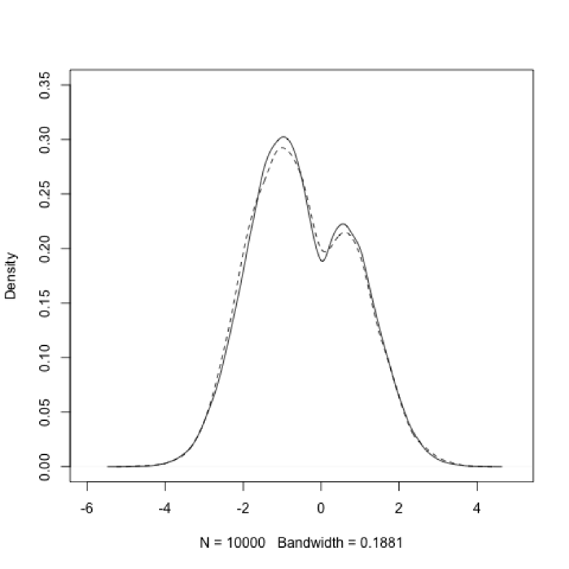
SDE$(1),a_{1}=0.2,a_{2}=-0.9$

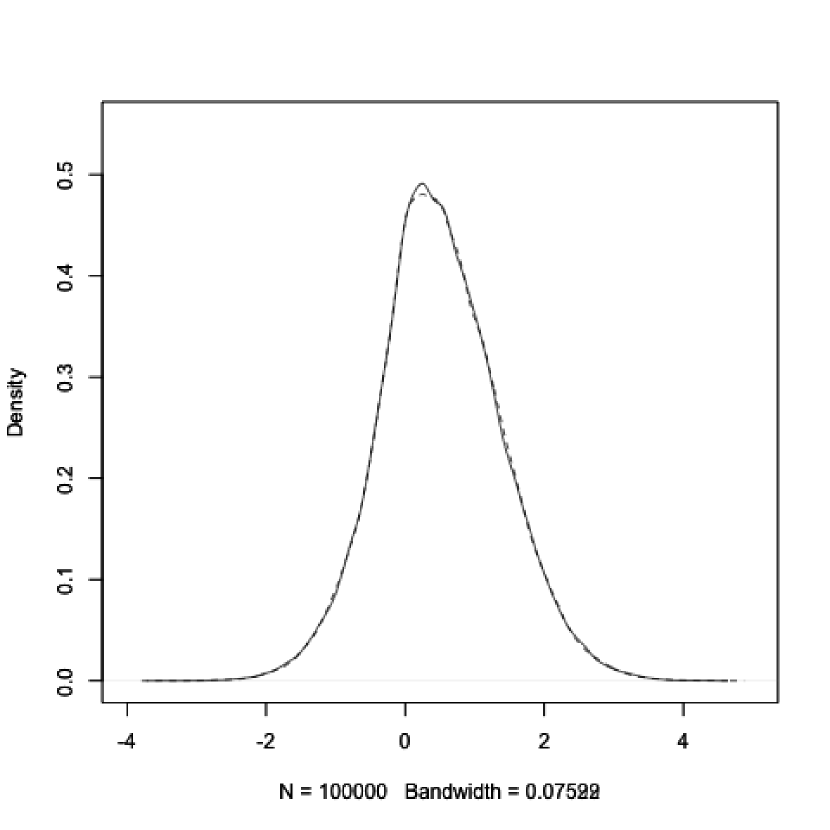
    SDE$(1),a_{1}=0.3,a_{2}=0.9$

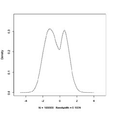
SDE (2), $\theta_{1}={7\over 6}\pi,\theta_{2}={1\over 4}\pi$

Figure 2: Kernel density estimation for $X$ at time $T=1$ using observations obtained by exact methods (solid line) and the Euler-Maruyama method (dashed line).

Appendix

Explicit formulas for $p_{1}(l_{1})$ and $p_{3}(l_{3})$ used in Section 2.3.

$$p_{1}(l_{1})= \mathbbm{1}_{b_{1}>0}c_{1}e^{-{(b_{1}+k_{1})^{2}\over 2(s_{3}-s_{1})}}[\sigma^{2}e^{-{\mu_{1}^{2}\over 2\sigma^{2}}}+\sqrt{2\pi}\sigma(\mu_{1}+k_{1})(1-\Phi_{\mu_{1},\sigma^{2}}(0))$$

$$-e^{{\mu_{2}^{2}-\mu_{1}^{2}\over 2\sigma^{2}}}(\sigma^{2}e^{-{\mu_{2}^{2}\over 2\sigma^{2}}}+\sqrt{2\pi}\sigma(\mu_{2}+k_{1})(1-\Phi_{\mu_{2},\sigma^{2}}(0)))]$$

$$+\mathbbm{1}_{b_{1}<0}c_{1}e^{-{(b_{1}-k_{1})^{2}\over 2(s_{3}-s_{1})}}[\sigma^{2}e^{-{\mu_{3}^{2}\over 2\sigma^{2}}}-\sqrt{2\pi}\sigma(\mu_{3}-k_{1})\Phi_{\mu_{3},\sigma^{2}}(0)$$

$$+e^{{\mu_{4}^{2}-\mu_{3}^{2}\over 2\sigma^{2}}}(-\sigma^{2}e^{-{\mu_{4}^{2}\over 2\sigma^{2}}}+\sqrt{2\pi}\sigma(\mu_{4}-k_{1})\Phi_{\mu_{4},\sigma^{2}}(0))]$$

$$p_{3}(l_{3})= \mathbbm{1}_{b_{3}>0}c_{2}e^{-{(b_{3}+k_{2})^{2}\over 2(s_{3}-s_{1})}}[\sigma^{2}e^{-{\nu_{1}^{2}\over 2\sigma^{2}}}+\sqrt{2\pi}\sigma(\nu_{1}+k_{2})(1-\Phi_{\nu_{1},\sigma^{2}}(0))$$

$$-e^{{\nu_{2}^{2}-\nu_{1}^{2}\over 2\sigma^{2}}}(\sigma^{2}e^{-{\nu_{2}^{2}\over 2\sigma^{2}}}+\sqrt{2\pi}\sigma(\nu_{2}+k_{2})(1-\Phi_{\nu_{2},\sigma^{2}}(0)))]$$

$$+\mathbbm{1}_{b_{3}<0}c_{2}e^{-{(b_{3}-k_{2})^{2}\over 2(s_{3}-s_{1})}}[\sigma^{2}e^{-{\nu_{3}^{2}\over 2\sigma^{2}}}-\sqrt{2\pi}\sigma(\nu_{3}-k_{2})\Phi_{\nu_{3},\sigma^{2}}(0)$$

$$+e^{{\nu_{4}^{2}-\nu_{3}^{2}\over 2\sigma^{2}}}(-\sigma^{2}e^{-{\nu_{4}^{2}\over 2\sigma^{2}}}+\sqrt{2\pi}\sigma(\nu_{4}-k_{2})\Phi_{\nu_{4},\sigma^{2}}(0))]$$

where

$$c_{1} =(f_{s_{3}-s_{1}}^{b_{1}}(b_{3},l_{3}-l_{1}))^{-1}(2\pi)^{-1}(s_{2}-s_{1})^{-{1\over 2}}(s_{3}-s_{2})^{-{3\over 2}}$$

$$c_{2} =(f_{s_{3}-s_{1}}^{b_{1}}(b_{3},l_{3}-l_{1}))^{-1}(2\pi)^{-1}(s_{2}-s_{1})^{-{3\over 2}}(s_{3}-s_{2})^{-{1\over 2}}$$

$$k_{1} =l_{3}-l_{1}+|b_{3}|\hskip 85.35826ptk_{2}=l_{3}-l_{1}+|b_{1}|$$

$$\mu_{1} ={b_{1}(s_{3}-s_{2})-k_{1}(s_{2}-s_{1})\over s_{3}-s_{1}}\hskip 28.45274pt\mu_{2}=\mu_{1}-2b_{1}{s_{3}-s_{2}\over s_{3}-s_{1}}$$

$$\mu_{3} ={b_{1}(s_{3}-s_{2})+k_{1}(s_{2}-s_{1})\over s_{3}-s_{1}}\hskip 28.45274pt\mu_{4}=\mu_{3}-2b_{1}{s_{3}-s_{2}\over s_{3}-s_{1}}$$

$$\nu_{1} ={b_{3}(s_{2}-s_{1})-k_{2}(s_{3}-s_{2})\over s_{3}-s_{1}}\hskip 28.45274pt\nu_{2}=\nu_{1}-2b_{3}{s_{2}-s_{1}\over s_{3}-s_{1}}$$

$$\nu_{3} ={b_{3}(s_{2}-s_{1})+k_{2}(s_{3}-s_{2})\over s_{3}-s_{1}}\hskip 28.45274pt\nu_{4}=\nu_{3}-2b_{3}{s_{2}-s_{1}\over s_{3}-s_{1}}$$

$$\sigma^{2}=(s_{2}-s_{1})(s_{3}-s_{2})(s_{3}-s_{1})^{-1}$$

References

- [BPR06] A. Beskos, O. Papaspiliopoulos, and G.O. Roberts. Retrospective exact simulation of diffusion sample paths with applications. Bernoulli, 12(6):1077, 2006.
- [BPR08] A. Beskos, O. Papaspiliopoulos, and G. O. Roberts. A factorisation of diffusion measure and finite sample path constructions. Methodology and Computing in Applied Probability, 10(1):85–104, 2008.
- [BR05] A. Beskos and G.O. Roberts. Exact simulation of diffusions. Annals of Applied Probability, 15(4):2422–2444, 2005.
- [BS02] A. N Borodin and P. Salminen. Handbook of Brownian motion: facts and formulae. Springer, 2002.
- [EM14] P. Etore and M. Martinez. Exact simulation for solutions of one-dimensional stochastic differential equations with discontinuous drift. ESAIM: Probability and Statistics, 18:686–702, 2014.
- [Tay15] K. B. Taylor. Exact Algorithms for simulation of diffusions with discontinuous drift and robust Curvature Metropolis-adjusted Langevin algorithms. PhD thesis, University of Warwick, 2015.
- [Zvo74] A. K. Zvonkin. A transformation of the state space of a diffusion process that annihilates the drift. Mat. Sb., Nov. Ser, 93(135):129–149, 1974.