Symmetric matrices, Catalan paths, and correlations

Abstract.

Kenyon and Pemantle (2014) gave a formula for the entries of a square matrix in terms of connected principal and almost-principal minors. Each entry is an explicit Laurent polynomial whose terms are the weights of domino tilings of a half Aztec diamond. They conjectured an analogue of this parametrization for symmetric matrices, where the Laurent monomials are indexed by Catalan paths. In this paper we prove the Kenyon-Pemantle conjecture, and apply this to a statistics problem pioneered by Joe (2006). Correlation matrices are represented by an explicit bijection from the cube to the elliptope.

1. Introduction

In this paper we present a formula for each entry of a symmetric $n\times n$ matrix $X=(x_{ij})$ as a Laurent polynomial in $\binom{n+1}{2}$ distinguished minors of $X$. Our result verifies a conjecture of Kenyon and Pemantle from [3]. Let $I$ and $J$ be subsets of $[n]=\{1,2,\dots,n\}$ with $|I|=|J|$. Let $X^{J}_{I}$ denote the minor of $X$ with row indices $I$ and column indices $J$. Here the indices in $I$ and $J$ are always taken in increasing order. The following signed minors will be used:

$$\,\,\begin{matrix}&p_{I}&:=&(-1)^{\lfloor\,|I|/2\,\rfloor}\cdot X_{I}^{I}&\\ {\rm and}&a_{ij|I}&:=&(-1)^{\lceil\,|I|/2\,\rceil}\cdot X^{jI}_{iI}&\,\,\,\hbox{for}\,\,\,i,j\not\in I,\quad i\neq j.\end{matrix}$$

We call $p_{I}$ and $a_{ij|I}$ the principal and almost-principal minors, respectively. The minors $p_{I}$, $a_{ij|I}$ and $a_{ji|I}$ are called connected if $1\leq i<j\leq n$ and $I=\{i{+}1,i{+}2,\dots,j{-}2,j{-}1\}$. The $1{\times}1$-minors $a_{ij}:=a_{ij|\emptyset}=x_{ij}$ and $p_{k}=x_{kk}$ are connected when $|i-j|=1$ and $1\leq k\leq n$.

These definitions make sense for every $n\times n$ matrix $X$, even if $X$ is not symmetric. A general $n{\times}n$ matrix $X$ has $2^{n}$ principal minors, of which $\binom{n-2}{2}+n$ are connected. It also has $n(n-1)2^{n-2}$ almost-principal minors, of which $n(n-1)$ are connected. A symmetric $n{\times}n$ matrix has $\binom{n}{2}2^{n-2}$ distinct almost-principal minors $a_{ij|I}$, of which $\binom{n}{2}$ are connected.

A Catalan path $C$ is a path in the $xy$-plane which starts at $(0,0)$ and ends on the $x$-axis, always stays at or above the $x$-axis, and consists of steps northeast $(1,1)$ and southeast $(1,-1)$. We say that $C$ has size $n$ if its endpoints have distance $2n-2$ from each other. Let $\mathscr{C}_{n}$ denote the set of Catalan paths of size $n$. Its cardinality equals the Catalan number

$$\qquad\quad|\mathscr{C}_{n}|\,=\,\frac{1}{n}\binom{2n-2}{n-1},\quad\hbox{which is}\,\,1,2,5,14,42,132,429,1430,4862\,\,\hbox{for $n=2,\ldots,10$}.$$

Let $G_{n}$ denote the planar graph whose vertices are the $\binom{n+1}{2}$ lattice points $(x,y)$ with $x\geq y\geq 0$ and $x+y\leq 2n-2$ even, and edges are northeast and southeast steps. Thus $\mathscr{C}_{n}$ consists of the paths from $(0,0)$ to $(2n-2,0)$ in $G_{n}$. We label the nodes and regions of $G_{n}$ as follows. We assign label $j$ to the node $(2j-2,0)$, label $a_{ij|I}$ to the node $(i+j-2,j-i)$, and label $p_{I}$ to the region below that node. Thus, connected principal and almost-principal minors of $X$ are identified in the graph $G_{n}$ with regions and nodes strictly above the $x$-axis.

The weight $W_{\mathscr{C}}(C)$ of a Catalan path $C$ is a Laurent monomial, derived from the drawing of $C$ in the graph ${G}_{n}$. Its numerator is the product of the labels $a_{ij|I}$ of the nodes of $G_{n}$ that are local maxima or local minima of $C$, and its denominator is the product of the labels $p_{I}$ of the regions which are either immediately below a local maximum or immediately above a local minimum. Thus $W_{\mathscr{C}}(C)$ is a Laurent monomial of degree $\leq 1$. There is no lower bound on the degree; for instance, $\frac{a_{13|2}a_{35|4}a_{57|6}a_{79|8}}{p_{2}p_{3}p_{4}p_{5}p_{6}p_{7}p_{8}}$ has degree $-3$ and appears for $n=9$.

The following result was conjectured by Kenyon and Pemantle in [3, Conjecture 1].

Theorem 1.1.

The entries of an $n\times n$ symmetric matrix $X=(x_{ij})$ satisfy the identity

(1) $$x_{ij}\,\,=\,\,\sum_{C}W_{\mathscr{C}}(C),$$

where the sum is over all Catalan paths $C$ between node $i$ and node $j$ in $G_{n}$

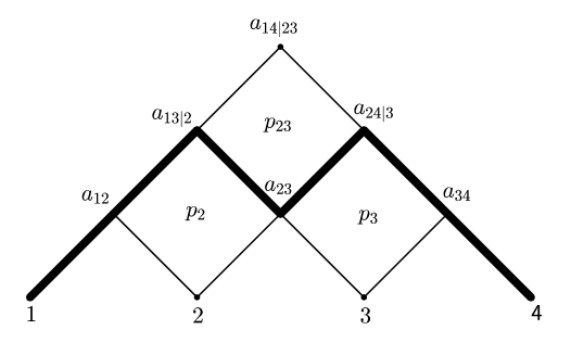
Figure 1. A Catalan path $C$ in the planar graph ${G}_{4}$ with weight $\frac{a_{13|2}a_{23}a_{24|3}}{p_{2}p_{23}p_{3}}$.

For symmetric matrices of size $n=4$, Theorem 1.1 states the following formula:

(2) $$X\,=\,\begin{pmatrix}\,p_{1}\,&\,a_{12}\,&\frac{a_{13|2}}{p_{2}}+\frac{a_{12}a_{23}\phantom{|}}{p_{2}}&\frac{a_{14|23}}{p_{23}}+\frac{a_{12}a_{24|3}}{p_{2}p_{3}}+\frac{a_{13|2}a_{34}}{p_{2}p_{3}}+\frac{a_{12}a_{23}a_{34}\phantom{|}}{p_{2}p_{3}}+\frac{a_{13|2}a_{23}a_{24|3}}{p_{2}p_{23}p_{3}}\vskip 3.0pt plus 1.0pt minus 1.0pt\\ \,*&p_{2}&a_{23}&\frac{a_{24|3}}{p_{3}}+\frac{a_{23}a_{34}\phantom{|}}{p_{3}}\vskip 3.0pt plus 1.0pt minus 1.0pt\\ \,*&*&p_{3}&a_{34}\vskip 3.0pt plus 1.0pt minus 1.0pt\\ \,*&*&*&p_{4}\end{pmatrix}$$

The entry $x_{14}=x_{41}$ is the sum of five Laurent monomials, one for each Catalan path from node $1$ to node $4$. The last term $\frac{a_{13|2}a_{23}a_{24|3}}{p_{2}p_{23}p_{3}}$ equals $W_{\mathscr{C}}(C)$ for the path $C$ shown in Figure 1.

The proof of Theorem 1.1 is given in Section 4. We start in Section 2 by reviewing a theorem of Kenyon and Pemantle [3] which expresses the entries of an arbitrary square matrix in terms of almost-principal and principal minors, as a sum of Laurent monomials that are in bijection with domino tilings of a half Aztec diamond. In Section 3, we give a bijection between these domino tilings and Schröder paths, and restate their theorem using Schröder paths. We then prove our theorem by constructing a projection from Schröder paths to Catalan paths and applying the relation (7) among minors of symmetric matrices.

In Section 5 we connect Theorem 1.1 to an application in statistics, developed in work of Joe, Kurowicka and Lewandowski [2, 5]. Namely, we focus on symmetric matrices that are positive definite and have all diagonal entries equal to $1$. These are the correlation matrices, and they form a convex set that is known in optimization as the elliptope [1, 4]. Our formula yields an explicit bijection between the elliptope and the open cube $(-1,1)^{\binom{n}{2}}$.

2. Square matrices and tilings of the half Aztec diamond

In this section we review the Kenyon-Pemantle formula in [3, Theorem 4.4]. The half Aztec diamond $HD_{n}$ of order $n$ is the union of the unit squares whose vertices are in the set

$$\{\,(a,b)\in\mathbb{Z}^{2}\,\,:\,\,\,|a|\leq n,\,0\leq b\leq n,\,|a|+|b|\leq n+1\,\}.$$

We label the boxes in the bottom row of $HD_{n}$ by the numbers $1$ through $2n$, from left to right. We label certain lattice points of $HD_{n}$ by minors as follows. Fix $b\in[n]$. The connected principal minors $p_{I}$ such that $|I|=b$ are assigned to the lattice points $(a,b)$ with $a+b$ even. The connected almost-principal minors $a_{ij|I}$ with $i>j$ and $|I|=b-1$ are assigned to the lattice points $(a,b)$ with $a+b$ odd. In both cases, the assignment is from left to right using the lexicographic order on $I$. The case $n=4$ is shown in Figure 2.

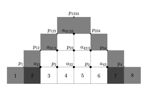
Figure 2. The half Aztec diamond $HD_{4}$. The white boxes are to be tiled.

Fix integers $a$ and $b$ such that $a$ is even, $b$ is odd, and $1{<}a{<}b{<}2n$. We define the colored half Aztec diamond $HD_{n}(a,b)$ by coloring the boxes of $HD_{n}$ black, grey, or white. First color boxes $a$ and $b$ in the bottom row black. Let $L_{a}$ be the diagonal line of slope $1$ through box $a-1$, and let $L_{b}$ be the line of slope $-1$ through box $b+1$. If a box (or any part of it) lies to the left of $L_{a}$ or to the right of $L_{b}$, then color it grey. All other boxes are white. A domino tiling (or simply a tiling) of $HD_{n}(a,b)$ is a tiling of the white boxes by $1{\times}2$ and $2{\times}1$ rectangles. Let $\mathscr{A}_{n}(a,b)$ denote the set of tilings of $HD_{n}(a,b)$. Figure 3 shows the set $\mathscr{A}_{4}(2,7)$, i.e. the six tilings of $HD_{4}(2,7)$, with lines $L_{2}$ and $L_{7}$ superimposed on the tilings.

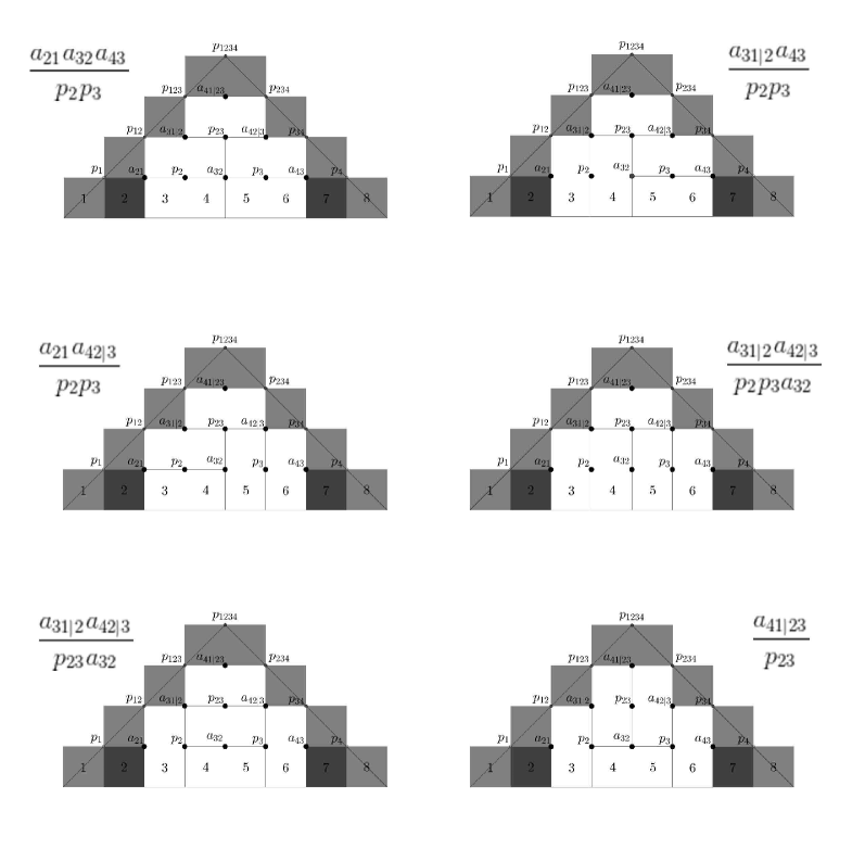
Figure 3. The six tilings of the colored half Aztec diamond $HD_{4}(2,7)$.

Each tiling $T$ of the colored half Aztec diamond $HD_{n}(a,b)$ gets a Laurent monomial weight, which we now define. We regard $T$ as a simple graph whose nodes are the lattice points of $HD_{n}$, and whose edges are induced by the edges of the rectangles in the tiling together with the edges of the unit squares outside the tiling. An interior lattice point of $HD_{n}(a,b)$ is a lattice point which lies strictly to the right of $L_{a}$ and strictly to the left of $L_{b}$. The interior lattice points that will concern us are shown in bold in Figures 2 and 3. Each of these is labeled by a variable $v_{\ell}$ which is a connected principal or almost-principal minor. The weight $W_{\mathscr{A}}(T)$ of a tiling $T\in\mathscr{A}_{n}(a,b)$ is defined to be the Laurent monomial

$$W_{\mathscr{A}}(T)\,\,:=\,\,\prod_{\ell}v_{\ell}^{d(\ell)-3},$$

where $\ell$ ranges over the interior lattice points of $HD_{n}(a,b)$ and $d(\ell)$ is the degree of $\ell$ in $T$.

Theorem 2.1 (Kenyon-Pemantle [3]).

The entries of an $n\times n$ matrix $X=(x_{ij})$ satisfy

$$x_{ij}\quad=\sum_{T\in\mathscr{A}_{n}(2j,2i-1)}W_{\mathscr{A}}(T)\qquad{\rm for}\,\,i>j.$$

Theorem 4.4 in [3] also gives a similar formula for $x_{ij}$ with $i<j$, but we omit that formula, as it is not needed here.

Example 2.2.

Figure 3 shows the six tilings of $HD_{4}(2,7)$ with their weights. By Theorem 2.1, the upper right matrix entry for $n=4$ is the sum of these six Laurent monomials:

(3) $$x_{41}\,\,=\,\,\frac{a_{21}a_{32}a_{43}}{p_{2}p_{3}}+\frac{a_{31|2}a_{43}}{p_{2}p_{3}}+\frac{a_{21}a_{42|3}}{p_{2}p_{3}}+\frac{a_{31|2}a_{42|3}}{p_{2}p_{3}a_{32}}+\frac{a_{31|2}a_{42|3}}{p_{23}a_{32}}+\frac{a_{41|23}}{p_{23}}.$$

The full $4\times 4$ matrix is shown on page 8 of [3], albeit with different notation.

3. Square matrices and Schröder paths

In this section we continue our discussion of arbitrary square matrices. A Schröder path $S$ is a path in the $xy$-plane which starts at $(0,0)$, always stays at or above the $x$-axis, and consists of steps which are either northeast $(1,1)$, southeast $(1,-1)$, or horizontal $(2,0)$. A Schröder path has order $n$ if it ends at $(2n-4,0)$. Let $G_{n}^{\prime}$ denote the planar graph whose nodes are the lattice points $(x,y)$ with $0\leq y\leq x$ and $x+y\leq 2n-4$ even, with edges given by northeast, southeast and horizontal steps. The set $\mathscr{S}_{n}$ of Schröder paths of order $n$ is identified with the left-to-right paths in $G_{n}^{\prime}$ from $(0,0)$ to $(2n-4,0)$. The cardinality of $\mathscr{S}_{n}$ is the Schröder number, which is given by the generating function

$$\sum_{n=2}^{\infty}|\mathscr{S}_{n}|z^{n-2}\,\,=\,\,\frac{1-z-\sqrt{1-6z+z^{2}}}{2z}\,=\,1+2z+6z^{2}+22z^{3}+90z^{4}+394z^{5}+1806z^{6}+\cdots$$

The graph $G_{n}^{\prime}$ is labeled by connected minors. We assign $a_{ij|I}$ to the node $(i{+}j{-}3,i{-}j{-}1)$ for $i>j$, and we assign $p_{I}$ to the triangle below that node. We refer to $(2i-2,0)$ as node $i$. Figure 4 shows the case $n=4$. The six Schröder paths in $\mathscr{S}_{4}$ are shown in Figure 6.

Figure 4. The graph $G^{\prime}_{4}$ encodes the Schröder paths of order $4$.

We now define the weight $W_{\mathscr{S}}(S)$ of a Schröder path $S$ on $G^{\prime}_{n}$. We regard $S$ as a graph with vertices $V(S)$ and edges $E(S)$. Given a Schröder path $S$ on $G^{\prime}_{n}$, we define the sets

$$\begin{matrix}\alpha(S)&=&\{v\in V(S):v\text{ is a weak local maximum of }S\},\qquad\qquad\qquad\qquad\,\,\\ \beta(S)&=&\{e\in E(S):e\text{ is immediately below a weak local minimum of }S\},\\ \gamma(S)&=&\{e\in E(S):e\text{ is a horizontal edge of }S\},\qquad\qquad\qquad\qquad\qquad\quad\\ \delta(S)&=&\{v\in V(S):v\text{ is immediately below a horizontal edge of }S\},\quad\quad\,\,\\ \epsilon(S)&=&\,\{e\in E(S):e\text{ is immediately below a strict local maximum of }S\},\\ \zeta(S)&=&\quad\,\,\,\{v\in V(S):v\text{ is a strict local minimum (but not an endpoint) of }S\}.\end{matrix}$$

Each of these is regarded as a monomial by taking the product of all labels. Then we define

(4) $$W_{\mathscr{S}}(S)\,\,=\,\,\frac{\alpha(S)\beta(S)}{\gamma(S)\delta(S)\epsilon(S)\zeta(S)}.$$

Figure 6 shows the six Schröder paths for $n=4$, together with their weights. The sum of these weights is the Laurent polynomial in (3), which evaluates to the matrix entry $x_{41}$.

The main result of this section is a reformulation of Theorem 2.1 in terms of Schröder paths. We write $\mathscr{S}_{n}(a,b)$ for the set of all Schröder paths from node $a$ to node $b$ in $G^{\prime}_{n}$.

Theorem 3.1.

The entries of an $n\times n$ matrix $X=(x_{ij})$ satisfy

$$x_{ij}\,\,\,\,=\sum_{S\in\mathscr{S}_{n}(j,i-1)}\!\!W_{\mathscr{S}}(S)\qquad{\rm for}\,\,\,i>j.$$

We shall present a weight-preserving bijection $\Phi:\mathscr{A}_{n}(2j,2i-1)\rightarrow\mathscr{S}_{n}(j,i-1)$ between tilings and Schröder paths. Note that we can superimpose the graph $G^{\prime}_{n}$ on the graph $HD_{n}$ so that the labels (connected minors) match up. When we do this, the vertex $j$ (respectively, $i-1$) of $G^{\prime}_{n}$ gets identified with the top right corner of the square $2j$ (respectively, the top left corner of the square $2i-1$) in $HD_{n}$. We draw a Schröder path $\Phi(T)$ on top of a tiling $T$, as in Figure 5. We may then think of the path as an element of $\mathscr{S}_{n}(j,i-1)$.

Figure 5. How to construct a Schröder path from a tiling.

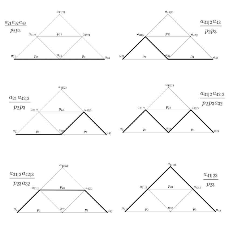
Figure 6. The six Schröder paths in $\mathscr{S}_{4}$ together with their weights.

More formally, given $T\in\mathscr{A}_{n}(2j,2i-1)$, the path $\Phi(T)\in\mathscr{S}_{n}(j,i-1)$ is defined as follows. Its starting point is the top right corner of square $2j$ in $HD_{n}(2j,2i-1)$. We inductively add steps to $\Phi(T)$ depending on the local behavior of the tiling, as shown in Figure 5. Let $x$ denote the endpoint of the path that we have built so far. Then we proceed as follows:

• If there is a vertical tile to the east of $x$, then we add a northeast step to our path.

• If there is a vertical tile to the southeast of $x$, such that $x$ is at its northwest corner, then we add a southeast step to our path.

• If there is a horizontal tile to the southeast of $x$, then add an east step to our path.

• If $x$ is already at the top left corner of square $2i-1$, then we stop.

The map $\Phi$ maps the six tilings in Figure 3 to the six Schröder paths in Figure 6.

Lemma 3.2.

The map $\Phi:\mathscr{A}_{n}(2j,2i-1)\to\mathscr{S}_{n}(j,i-1)$ is well-defined and is a bijection.

Proof.

This is the solution to Exercise 6.49 in [7], based on an idea of Dana Randall. ∎

Proposition 3.4 states that this bijection is weight-preserving. First, another lemma:

Lemma 3.3.

The local move shown in the top of Figure 7 alters the weight of both the tiling and the corresponding Schröder path by the same factor: when passing from the left to the right, the exponents of $b$ and $h$ increase by $1$, while those of $d$ and $f$ decrease by $1$.

Figure 7. A flip of a tiling and the corresponding local move on Schröder paths.

Proof.

The statement is clear by inspection for the tilings. Checking the assertion for Schröder paths is more complicated. We need to examine the various cases of what the path looks like on the left and right of the square being modified. In other words, we need to specify whether the path increases, stays flat or decreases as it enters node $d$, and ditto for when it leaves node $f$. One such case is seen in Figure 8. When we perform that local move, the exponents of $b$ and $h$ in (4) increase by $1$, while the exponents of both $d$ and $f$ decrease by $1$. All other cases are similar. ∎

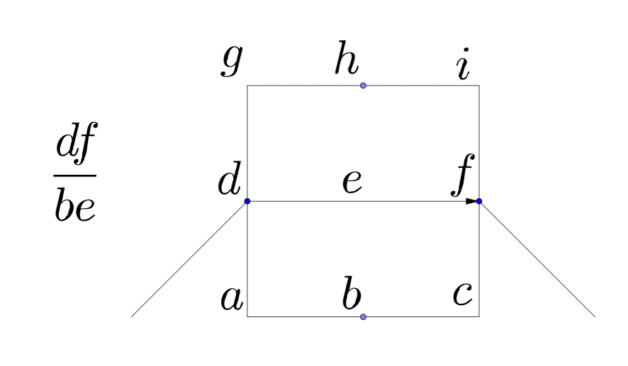
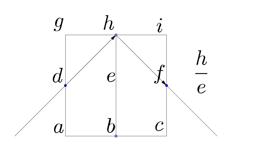
Figure 8. This local move multiplies the weight of the Schröder path by $\frac{bh}{df}$.

Proposition 3.4.

If $T$ is a tiling in $\mathscr{A}_{n}(2j,2i-1)$, where $i>j$, then $W_{\mathscr{S}}(\Phi(T))=W_{\mathscr{A}}(T)$.

Proof.

It is well known [6] that two domino tilings of a simply connected region can always be connected by a sequence of flips, where a flip is the local move that switches two horizontal tiles for two vertical tiles or vice-versa, as seen in Figure 7.

Let $T_{0}$ be the tiling consisting only of horizontal tiles. The corresponding Schröder path $\Phi(T_{0})$ is a horizontal path. Here, the two objects have the same weight:

(5) $$W_{\mathscr{S}}(\Phi(T_{0}))\,=\,W_{\mathscr{A}}(T_{0})\,=\,\frac{a_{j+1,j}a_{j+2,j+1}a_{j+3,j+2}\dots a_{i,i-1}}{p_{j+1}p_{j+2}p_{j+3}\dots p_{i-1}}.$$

By Lemma 3.3, if $W_{\mathscr{S}}(\Phi(T))=W_{\mathscr{A}}(T)$ and $T^{\prime}$ is obtained by a flip, then $W_{\mathscr{S}}(\Phi(T^{\prime}))=W_{\mathscr{A}}(T^{\prime})$. Since the tilings in $\mathscr{A}_{n}(2j,2i{-}1)$ are connected by flips, the assertion follows. ∎

Proof of Theorem 3.1.

This follows from Theorem 2.1, Lemma 3.2 and Proposition 3.4. ∎

4. Back to symmetric matrices

The strategy for proving Theorem 1.1 is to combine Theorem 3.1 with a projection from Schröder paths to Catalan paths. Let $S$ be any Schröder path in $G^{\prime}_{n}$. The associated Catalan path $\pi(S)$ in $G_{n}$ is defined by

• replacing each horizontal step in $S$ with a strict local minimum, i.e. a southeast step followed by a northeast step;

• adding a northeast step at the beginning of $S$ and a southeast step at the end of $S$.

If $S$ starts at $i$ and ends at $j-1$ in $G^{\prime}_{n}$ then $\pi(S)$ starts at $i$ and ends at $j$ in $G_{n}$. Figure 9 shows how four of the six Schröder paths in $\mathscr{S}_{4}(1,3)$ map to four of the five Catalan paths in $\mathscr{C}_{4}(1,4)$. The two other Schröder paths in Figure 6 map to the Catalan path in Figure 1.

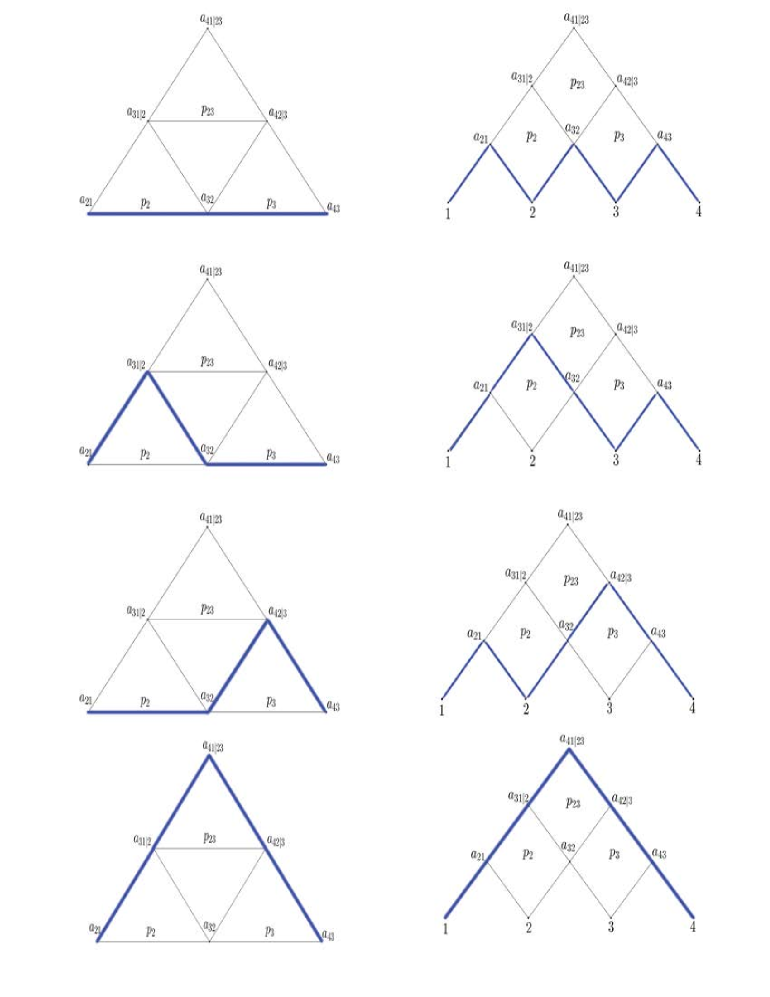
Figure 9. The Schröder paths (left) are projected to the Catalan paths (right).

Theorem 2.1 is an immediate consequence of Theorem 3.1 and the following proposition.

Proposition 4.1.

The weight of a Catalan path is the sum of the weights of the Schröder paths in its preimage under the projection $\pi$, i.e.

(6) $$\sum_{S\in\pi^{-1}(C)}\!\!W_{\mathscr{S}}(S)\,\,=\,\,W_{\mathscr{C}}(C).$$

Here the labels of the paths come from a symmetric matrix, i.e. $x_{ij}=x_{ji}$ for all $i$ and $j$.

The proof will rely on equation (7) and Lemma 4.2. Using Muir’s law of extensible minors, we obtain the following identity that expresses connected almost-principal minors of a symmetric $n\times n$ matrix in terms of connected principal minors:

(7) $$\qquad a_{ij|I}^{2}\,-\,p_{I}p_{I\cup\{i,j\}}-p_{I\cup\{i\}}p_{I\cup\{j\}}\,\,=\,\,0,\qquad 2\leq i<j\leq n{-}1,\,\,I=\{i{+}1,\ldots,j{-}1\}.$$

We now use this identity to prove the following claim.

Lemma 4.2.

Let $S^{\prime}$ and $S$ be two Schröder paths in $\mathscr{S}_{n}$ that are related as shown in the bottom row of Figure 7 (with $S^{\prime}$ on the left and $S$ on the right). If the labels come from a symmetric $n\times n$ matrix, then the resulting weights of these paths satisfy

(8) $$W_{\mathscr{S}}(S)\,+\,W_{\mathscr{S}}(S^{\prime})\,\,=\,\,\frac{e^{2}}{bh}W_{\mathscr{S}}(S).$$

Proof.

The label $e$ of the local minimum in $S$ is an almost-principal minor, while $b,h,d,f$ are principal minors. By (7), it satisfies $\,e^{2}=bh+df$, and hence $\frac{e^{2}}{bh}=1+\frac{df}{bh}$. By Lemma 3.3, we have $W_{\mathscr{S}}(S^{\prime})=\frac{df}{bh}W_{\mathscr{S}}(S).$ This implies $\,\frac{e^{2}}{bh}W_{\mathscr{S}}(S)\,=\,W_{\mathscr{S}}(S)+W_{\mathscr{S}}(S^{\prime})$. ∎

Example 4.3.

Let $S^{\prime}$ and $S$ be the fourth and fifth Schröder paths in Figure 6, with labels given by a symmetric $4{\times}4$ matrix. Using the identity $a_{23}=p_{23}+p_{2}p_{3}$, as in (7), we find

$$W_{\mathscr{S}}(S)\,+\,W_{\mathscr{S}}(S^{\prime})\,\,=\,\,\frac{a_{13|2}a_{24|3}}{p_{2}p_{3}a_{23}}\,+\frac{a_{13|2}a_{24|3}}{p_{23}a_{23}}\,\,=\,\,\frac{a_{13|2}a_{24|3}a_{23}}{p_{2}p_{23}p_{3}}.$$

This explains how the six terms in (3) become the five terms of $x_{14}$ shown in (2). Namely, the weight of the Catalan path in Figure 1 is the sum of the fourth and fifth terms in (3).

Proof of Proposition 4.1.

Let $C$ be a Catalan path with $m$ local minima. It has $m+1$ local maxima. Let $A_{1},\dots,A_{m}$ and $A^{\prime}_{1},\dots,A^{\prime}_{m+1}$ denote the variables at the local minima and maxima, respectively. Let $P_{1},\dots,P_{m}$ and $P^{\prime}_{1},\dots,P^{\prime}_{m+1}$ denote the face variables located directly above the minima and directly below the maxima, respectively. Then

(9) $$W_{\mathscr{C}}(C)\,\,=\,\,\frac{A_{1}\cdots A_{m}A^{\prime}_{1}\cdots A^{\prime}_{m+1}}{P_{1}\cdots P_{m}P^{\prime}_{1}\cdots P^{\prime}_{m+1}}.$$

We also denote the face variables located directly below the local minima by $P^{\prime\prime}_{1},\dots,P^{\prime\prime}_{m}$.

There are $2^{m}$ Schröder paths that project to $C$ via $\pi$. These correspond to the $2^{m}$ choices of either preserving a local minimum, or replacing it by a horizontal edge. We denote the Schröder paths in $\pi^{-1}(C)$ by $S_{d_{1}d_{2}\dots d_{m}}$, where $d_{i}=0$ if the local minimum at $A_{i}$ was preserved and $d_{i}=1$ if it was replaced by a horizontal edge. By Lemma 4.2, we have

$$\begin{matrix}W_{\mathscr{S}}(S_{0d_{2}\cdots d_{m}})+W_{\mathscr{S}}(S_{1d_{2}\cdots d_{m}})&=&\frac{A_{1}^{2}}{P_{1}P^{\prime\prime}_{1}}W_{\mathscr{S}}(S_{0d_{2}\cdots d_{m}}),\qquad\\ W_{\mathscr{S}}(S_{d_{1}0d_{3}\cdots d_{m}})+W_{\mathscr{S}}(S_{d_{1}1d_{3}\cdots d_{m}})&=&\frac{A_{2}^{2}}{P_{2}P^{\prime\prime}_{2}}W_{\mathscr{S}}(S_{d_{1}0d_{3}\cdots d_{m}}),\ldots\end{matrix}$$

By aggregating these identities, we obtain

$$\sum_{S\in\pi^{-1}(C)}\!\!\,W_{\mathscr{S}}(S)\,\,=\,\,\sum_{d_{1},\ldots,d_{m}\in\{0,1\}}\!\!\!\!W_{\mathscr{S}}(S_{d_{1}d_{2}\cdots d_{m}})\,\,=\,\,\frac{A_{1}^{2}A_{2}^{2}\cdots A_{m}^{2}}{P_{1}P^{\prime\prime}_{1}P_{2}P^{\prime\prime}_{2}\cdots P_{m}P^{\prime\prime}_{m}}W_{\mathscr{S}}(S_{00\dots 0}).$$

But, now it follows from (4) and (9) that

$$W_{\mathscr{S}}(S_{00\dots 0})\,\,=\,\,\frac{A^{\prime}_{1}\cdots A^{\prime}_{m+1}P^{\prime\prime}_{1}\cdots P^{\prime\prime}_{m}}{P^{\prime}_{1}\cdots P^{\prime}_{m+1}A_{1}\cdots A_{m}}\,\,\,=\,\,\,\frac{P_{1}P^{\prime\prime}_{1}P_{2}P^{\prime\prime}_{2}\cdots P_{m}P^{\prime\prime}_{m}}{A_{1}^{2}A_{2}^{2}\cdots A_{m}^{2}}W_{\mathscr{C}}(C).$$

Therefore the sum of the weights of the Schröder paths in $\pi^{-1}(C)$ is equal to $W_{\mathscr{C}}(C)$. ∎

Remark 4.4.

The expression in Theorem 1.1 is not the only way to express the entries of a symmetric matrix in terms of the $\binom{n}{2}+\binom{n-2}{2}+n$ connected almost-principal and principal minors. The ideal of polynomial relations among these minors is generated by the $\binom{n-2}{2}$ quadrics in (7). Indeed, Theorem 1.1 ensures that the algebra generated by these minors has dimension $\binom{n+1}{2}$, so their relation ideal has codimension $\binom{n-2}{2}=\binom{n}{2}+\binom{n-2}{2}+n-\binom{n+1}{2}$. The $\binom{n-2}{2}$ relations (7) lie in that ideal and they generate a complete intersection. That complete intersection is a prime ideal because none of the $a_{ij|I}$ lie in the subalgebra generated by the principal minors. For instance, for $n=4$, our prime ideal is principal. It is $\langle a_{23}^{2}-p_{2}p_{3}-p_{23}\rangle$.

5. Parametrizing Correlation Matrices

We now specialize to real symmetric $n\times n$ matrices that are positive definite and have all diagonal entries equal to $1$. Such matrices are known as correlation matrices. They play an important role in statistics, notably in the study of multivariate normal distributions. The set $\mathcal{E}_{n}$ of all $n\times n$ correlation matrices is an open convex set of dimension $\binom{n}{2}$. Its closure is a convex body, known in optimization theory [1, 4] under the name elliptope.

In certain statistical applications it is desirable to generate random correlation matrices. Specifically, one wishes to sample from the uniform distribution on the elliptope $\mathcal{E}_{n}$. A solution to this problem was given by Joe [2] and further refined by Lewandowski et al. [5]. The underlying geometric idea is to construct a parametrization from the standard cube:

$$\Psi:(-1,1)^{\binom{n}{2}}\rightarrow\mathcal{E}_{n}.$$

The papers [2, 5] describe such maps $\Psi$ that are algebraic and bijective, so they identify the open cube with the open elliptope. However, the construction is recursive. In what follows we revisit the formula in [2] and we make it completely explicit. Remarkably, it is precisely the restriction of our Laurent polynomial parametrization in Theorem 1.1 to the region where all connected principal minors $p_{I}$ are positive and $p_{1}=\cdots=p_{n}=1$.

Let $X=(x_{ij})$ be a real symmetric $n\times n$ matrix. We assume that $X$ is positive definite, i.e. all principal minors $p_{I}$ are strictly positive. In statistics, such an $X$ serves as the covariance matrix of a normal distribution on $\mathbb{R}^{n}$, whose partial correlations are given by

(10) $$\qquad\rho_{ij|I}\,\,=\,\,\frac{(-1)^{\lceil\,|I|/2\,\rceil}\cdot a_{ij|I}}{\sqrt{p_{iI}\cdot p_{jI}}}\qquad\hbox{where}\,\,\,i,j\not\in I\,\,\hbox{and}\,\,i<j.$$

For $I=\emptyset$, we obtain the $\binom{n}{2}$ entries of the correlation matrix $Y=(y_{ij})$, namely

$$y_{ij}\,=\,\rho_{ij}\,=\,\frac{a_{ij}}{\sqrt{p_{i}p_{j}}}\,=\,\frac{x_{ij}}{\sqrt{x_{ii}x_{jj}}}\qquad\hbox{for}\,\,1\leq i<j\leq n.$$

The partial correlation $\rho_{ij|I}$ in (10) is called connected if $I=\{i{+}1,i{+}2,\dots,j{-}2,j{-}1\}$.

Theorem 5.1.

The $\binom{n}{2}$ entries $y_{ij}$ of a correlation matrix can be written uniquely in terms of the $\binom{n}{2}$ connected partial correlations $\rho_{ij|I}$. Explicit formulas are derived from those in Theorem 1.1 by first replacing each occurrence of a parameter $\,a_{ij|I}\,$ by $\,(-1)^{\lceil\,|I|/2\,\rceil}\rho_{ij|I}\sqrt{p_{iI}p_{jI}}\,$ and thereafter replacing each occurrence of a parameter $\,p_{r,r+1,\ldots,s}\,$ by the product of the $\binom{s-r+1}{2}$ expressions $\,(-1)^{\lfloor\,|I|/2\,\rfloor}(1-\rho_{ij|I}^{2})\,$ where $r{\leq}i{<}j{\leq}s$ and $\,I=\{i{+}1,i{+}2,\ldots,j{-}1\}$. The resulting map $\Psi:(\rho_{ij|I})\mapsto(y_{ij})$ is a bjection between $(-1,1)^{\binom{n}{2}}$ and $\,\mathcal{E}_{n}$.

Proof.

The replacement formula for $a_{ij|I}$ is seen in (10). The formula for the signed principal minors $\,p_{r,r+1,\ldots,s}\,$ in terms of connected partial correlations is due to Joe [2, Theorem 1]. It can be derived by recursively applying the following version of (7) in concert with (10):

(11) $$p_{ijI}\,\,=\,\,\frac{a_{ij|I}^{2}-p_{iI}p_{jI}}{p_{I}},\quad I=\{i+1,\ldots,j-1\}.$$

Our formulas give an algebraic map $\Psi:(\rho_{ij|I})\mapsto(y_{ij})$ between affine spaces of dimension $\binom{n}{2}$. This map is invertible on $\mathcal{E}_{n}$ because each partial correlation $\rho_{ij|I}$ can be written via (10) in terms of the entries $y_{ij}$ of the correlation matrix. All partial correlations are real numbers strictly between $-1$ and $1$. The connected partial correlations $\rho_{ij|I}$ can vary freely, as explained in [2, page 2179]. From this, we get the desired bijection. ∎

We now illustrate our parametrization of correlation matrices in the two smallest cases.

Example 5.2 ($n=3$).

We consider the open $3$-dimensional cube defined by the inequalities

$$-1\,\,<\,\,\rho_{12},\,\rho_{23},\,\rho_{13|2}\,\,<\,\,1.$$

Our bijection $\Psi$ identifies each point in this cube with a $3\times 3$ correlation matrix:

$$\!\begin{bmatrix}1&y_{12}&y_{13}\\ y_{12}&1&y_{23}\\ y_{13}&y_{23}&1\end{bmatrix}=\,\begin{bmatrix}1&\rho_{12}&\rho_{12}\rho_{23}-\rho_{13|2}(1{-}\rho_{12}^{2})^{\frac{1}{2}}(1{-}\rho_{23}^{2})^{\frac{1}{2}}\\ \,\rho_{12}\,&1&\rho_{23}\\ \rho_{12}\rho_{23}-\rho_{13|2}(1{-}\rho_{12}^{2})^{\frac{1}{2}}(1{-}\rho_{23}^{2})^{\frac{1}{2}}&\rho_{23}&1\end{bmatrix}.$$

One checks that this matrix is positive definite, and, as in [2, Theorem 1], its determinant

$${\rm det}(Y)\,\,=\,\,(1-\rho_{12}^{2})(1-\rho_{23}^{2})(1-\rho_{13|2}^{2})$$

defines the facets of the cube. It is instructive to draw how the boundary of the cube maps onto the boundary of the elliptope $\mathcal{E}_{3}$. The latter is depicted in [1, Figure 5.8, page 232].

The combinatorics of our planar graph $G_{n}$ and its Catalan paths can be seen in a different guise in [2, 5]. These correspond to the structures called D-vines in these papers. Figure 10 shows the standard D-vine for $n=4$. Its edges are naturally labeled with the six coordinates of the cube, namely $\rho_{12},\rho_{23},\rho_{34},\rho_{13|2},\rho_{24|3},\rho_{14|23}$. These correspond to the six almost-principal minors $a_{ij|I}$ in the labeled graph $G_{4}$ in Figure 1.

Figure 10. The standard D-vine for four random variables.

Example 5.3 ($n=4$).

The $4{\times}4$ correlation matrix $Y$ is obtained from the matrix $X$ in (2) by performing the replacements that are described in Theorem 5.1. We first substitute

$$\begin{matrix}a_{12}=\rho_{12}\sqrt{p_{1}p_{2}},&a_{23}=\rho_{23}\sqrt{p_{2}p_{3}},&a_{34}=\rho_{34}\sqrt{p_{3}p_{4}},\\ a_{13|2}=-\rho_{13|2}\sqrt{p_{12}p_{23}},&a_{24|3}=-\rho_{24|3}\sqrt{p_{23}p_{34}},&a_{14|23}=-\rho_{14|23}\sqrt{p_{123}p_{234}},\end{matrix}$$

and then we eliminate the connected principal minors as follows:

$$\begin{matrix}p_{1}=1,\,p_{2}=1,\,p_{3}=1,\,p_{4}=1,\,p_{12}=-(1-\rho_{12}^{2}),\,p_{23}=-(1-\rho_{23}^{2}),\,p_{34}=-(1-\rho_{34}^{2}),\\ p_{123}=-(1-\rho_{12}^{2})(1-\rho_{23}^{2})(1-\rho_{13|2}^{2})\quad{\rm and}\quad p_{234}=-(1-\rho_{23}^{2})(1-\rho_{34}^{2})(1-\rho_{24|3}^{2}).\end{matrix}$$

This results in the formulas for the six entries of $Y$ in terms of $\rho_{12},\rho_{23},\rho_{34},\rho_{13|2},\rho_{24|3},\rho_{14|23}$. These give the bijection $\Psi$ between the cube and the elliptope, both of dimension six. It is instructive to verify that ${\rm det}(Y)$ is the product of the facet-defining expressions $(1-\rho_{\bullet})^{2}$.

The paper [5] argues that C-vines are better than D-vines when it comes to sampling from the elliptope $\mathcal{E}_{n}$. It would be interesting to examine both C-vines and D-vines from the network perspective of [3] and to explore whether Catalan-type formulas for $X$ can be derived from these as well. Could such vines play a role in the theory of cluster algebras?

Acknowledgements. We thank Richard Kenyon, Robin Pemantle and Caroline Uhler for helpful conversations. This project was supported by the National Science Foundation (DMS-1419018, DGE-1106400, DMS-1049513).

Authors’ address:

Department of Mathematics, University of California, Berkeley, CA 94720-3840, USA

$\{$bernd,e.tsukerman,williams$\}$@math.berkeley.edu

References

[1]
Grigoriy Blekherman, Pablo Parrilo and Rekha Thomas:
Semidefinite Optimization and Convex Algebraic Geometry,
MOS-SIAM Ser. Optim., 13, SIAM, Philadelphia, PA, 2013.
[2]
Harry Joe:
Generating random correlation matrices based on partial correlations,
J. Multivariate Anal., 97(10):2177–2189, 2006.
[3]
Richard Kenyon and Robin Pemantle:
Principal minors and rhombus tilings,
J. Phys. A: Math. Theor., 47:474010, 2014.
[4] Monique Laurent and Svatopluk Poljak:
On the facial structure of the set of correlation matrices,
SIAM J. Matrix Anal. Appl. 17: 530–547, 1996.
[5]
Daniel Lewandowski, Dorota Kurowicka, and Harry Joe:
Generating random correlation matrices based on vines and extended
onion method,
J. Multivariate Anal., 100(9):1989–2001, 2009.
[6]
Nicolau Saldanha and Carlos Tomei:
An overview of domino and lozenge tilings,
Resenhas IME-USP, 2(2):239–252, 1995.
[7]
Richard P. Stanley:
Enumerative Combinatorics, Vol. 2, volume 62 of Cambridge Studies in Advanced Mathematics,
Cambridge University Press, 1999.