Seeing the Unseen Network:
Inferring Hidden Social Ties from Respondent-Driven Sampling

Lin Chen1,2    Forrest W. Crawford2,3    Amin Karbasi1,2
1Department of Electrical Engineering, 2Yale Institute for Network Science, 3Department of Biostatistics
Yale University, New Haven, CT 06520
{lin.chen, forrest.crawford, amin.karbasi}@yale.edu
Abstract

Learning about the social structure of hidden and hard-to-reach populations — such as drug users and sex workers — is a major goal of epidemiological and public health research on risk behaviors and disease prevention. Respondent-driven sampling (RDS) is a peer-referral process widely used by many health organizations, where research subjects recruit other subjects from their social network. In such surveys, researchers observe who recruited whom, along with the time of recruitment and the total number of acquaintances (network degree) of respondents. However, due to privacy concerns, the identities of acquaintances are not disclosed. In this work, we show how to reconstruct the underlying network structure through which the subjects are recruited. We formulate the dynamics of RDS as a continuous-time diffusion process over the underlying graph and derive the likelihood of the recruitment time series under an arbitrary inter-recruitment time distribution. We develop an efficient stochastic optimization algorithm called Render (REspoNdent-Driven nEtwork Reconstruction) that finds the network that best explains the collected data. We support our analytical results through an exhaustive set of experiments on both synthetic and real data.

Introduction

Random sampling is an effective way for researchers to learn about a population of interest. Characteristics of the sample can be generalized to the population of interest using standard statistical theory. However, traditional random sampling may be impossible when the target population is hidden, e.g. drug users, men who have sex with men, sex workers and homeless people. Due to concerns like privacy, stigmatization, discrimination, and criminalization, members of hidden populations may be reluctant to participate in a survey. In addition to the hidden populations for which no sampling “frame” exists, there are rare populations of great research interest, marked by their tiny fractions in the entire population. It is unlikely that random sampling from the general population would accrue a reasonable sample from a very rare population. However, it is often the case that members of hidden or rare populations know each other socially. This suggests that social referral would be an effective method for accruing a large sample. To this end, researchers have developed a variety of social link-tracing survey designs. The most popular is respondent-driven sampling (RDS) (?).

In RDS, a small set of initial subjects, known as “seeds” are selected, not necessarily simultaneously, from the target population. Subjects are given a few coupons, each tagged with a unique identifier, which they can use to recruit other eligible subjects. Participants are given a reward for being interviewed and for each eligible subject they recruit using their coupons. Each subject reports their degree, the number of others whom they know in the target population. No subject is permitted to enter the study twice and the date and time of each interview is recorded.

While RDS can be an effective recruitment method, it reveals only incomplete social network data to researchers. Any ties between recruited subjects along which no recruitment took place remain unobserved. The social network of recruited subjects is of great interest to sociologists, epidemiologists and public health researchers since it may induce dependencies in the outcomes of sampled individuals. Fortunately, RDS reveals information about the underlying social network that can be used to (approximately) reconstruct it. By leveraging the time series of recruitments, the degrees of recruited subjects, coupon information, and who recruited whom, it is possible to interpret the induced subgraph of RDS respondents as a simple random graph model (?).

In this paper, we introduce a flexible and expressive stochastic model of RDS recruitment on a partially observed network structure. We derive the likelihood of the observed time series; the model admits any edgewise inter-recruitment time distribution. We propose a stochastic optimization algorithm Render (REspoNdent-Driven nEtwork Reconstruction) to estimate unknown parameters and the underlying social network. We conduct extensive experiments, on synthetic and real data, to confirm the accuracy and the reconstruction performance of Render. In particular, we apply Render to reconstruct the network of injection drug users from an RDS study in St. Petersburg, Russia.

Related Work

RDS has been modeled as a random walk with replacement on a graph at its equilibrium distribution (?????), and under this argument the sampling probability is proportional to degree, which is the basis for an estimator of the population mean (??). In this paper, we adopt an approach that focuses on the network structure estimable from the RDS sample using recruitment information (?). ? (2016) assumes that edge-wise inter-recruitment times follow the exponential distribution, but this approach is relatively inflexible. In many other contexts, dynamic or random processes can reveal structural information of an underlying, partially observed, network (???). Network reconstruction and the edge prediction problem have been studied for diffusion processes where multiple realizations of the process on the same network are available (???). In the case of RDS, reconstruction is particularly challenging because only a single realization of the diffusion process is observed. Furthermore, we must account for the role of coupons in recruitment as they intricately introduce bias. However, in contrast to general diffusion processes over graphs, some important network topological information is revealed by RDS. In this study, we leverage all the available data routinely collected during real-world RDS studies.

Problem Formulation

We conform to the following notation throughout the paper. Suppose that $f$ is a real-valued function and that $\mathbf{v}$ is a vector. Then $f(\mathbf{v})$ is a vector of the same size as vector $\mathbf{v}$ and the $i$-th entry of $f(\mathbf{v})$ is denoted by $f(\mathbf{v})_{i}$, whose value is given by $f(\mathbf{v}_{i})$. The transposes of matrix $\mathbf{A}$ and vector $\mathbf{v}$ are written as $\mathbf{A}^{\prime}$ and $\mathbf{v}^{\prime}$, respectively. And let $\mathbf{1}$ be the all-ones column vector.

Dynamics of Respondent-Driven Sampling

We characterize the social network of the hidden population as a finite undirected simple graph $G=(V,E)$ with no parallel edges or self-loops. Members of the hidden population are vertices; $\{i,j\}\in E$ implies that $i\in V$ and $j\in V$ know each other. Using RDS, researchers recruit members from the hidden population into the study. The time-varying recruitment-induced subgraph $\{G_{S}(t)=(V_{S}(t),E_{S}(t)):0\leq t\leq t_{F}\}$ is a nested collection of subgraphs of $G$, where $t_{F}$ is the termination time of the study. For all $0\leq t\leq t_{F}$, $G_{S}(t)$ is a subgraph of $G$. Here, $G_{S}(0)$ is the null graph since there are no subjects in the study initially. For simplicity, we write $G_{S}=(V_{S},E_{S})$ for $G_{S}(t_{F})=(V_{S}(t_{F}),E_{S}(t_{F}))$, and call this the recruitment-induced subgraph or induced subgraph unless we explicitly specify the time $t$. The vertex set of the time-varying recruitment-induced subgraph at time $t$ (i.e., $G_{S}(t)$) denotes the members in the hidden population that are known to the study by time $t$. The subgraph $G_{S}(t)$ is induced by the vertex set $V_{S}(t)$; i.e., $E_{S}(t)=\{\{i,j\}|i,j\in V_{S}(t),\{i,j\}\in E\}$. The time-varying recruitment-induced subgraph evolves in the following way (?).

  1. 1.

    At time $\tilde{t}$, researchers recruit a subject in the population as a seed. This subject is included in the vertex set $V_{S}(t)$ of $G_{S}(t)$ for all $t\geq\tilde{t}$. Researchers may provide this subject with coupons to recruit its neighbors.

  2. 2.

    Once recruited into this study (either by researchers or its neighbors) at time $\tilde{t}$, subjects currently holding coupons will attempt to recruit their yet-unrecruited neighbors. The inter-recruitment time along each edge connecting a recruiter with an unrecruited neighbor is i.i.d. with cdf $F(t)$. Recruitment happens when a neighbor is recruited into the study and is provided with a number of coupons. A successful recruitment costs the recruiter one coupon.

The directed recruitment graph is $G_{R}=(V_{R},E_{R})$, where $V_{R}=V_{S}(t_{F})$ is the set of members in the study at the final stage. For two subjects $i,j\in V_{R}$, $(i,j)\in E_{R}$ if and only if $i$ recruits $j$. Note that the subjects recruited by researchers (i.e., the seeds) have zero in-degree in $G_{R}$. Let $n$ denote the cardinality of $V_{R}$ (equivalently $V_{S}(t_{F})$). For simplicity, we label the subject recruited in the $i$th recruitment event by $i$. The labels of the subjects in the study are $1,2,3,\ldots,n$. The vector of recruitment times is $\mathbf{t}=(t_{1},t_{2},t_{3},\ldots,t_{n})$, where $t_{i}$ is the recruitment time of subject $i$. In shorthand, we write $\tau(i;j)=t_{j-1}-t_{i}$ for $i<j$. Let $\mathbf{C}$ be the $n\times n$ coupon matrix whose element $\mathbf{C}_{ij}=1$ if subject $i$ has at least one coupon just before the $j$th recruitment event, and zero otherwise. The rows and columns of the coupon matrix are ordered by subjects’ recruitment time. The degree vector is $\mathbf{d}=(d_{1},d_{2},d_{3},\ldots,d_{n})^{\prime}$, where $d_{i}$ is the degree of $i$ in $G$. At time $t$ (where $t\neq t_{i}$ for $i=1,2,3,\ldots,n$), if a subject has at least one coupon and at least one neighbor not in the study, we term it a recruiter at time $t$; if a subject has not entered the study and has at least one neighbor with at least one coupon, we term it a potential recruitee at time $t$. We assume that the observed data from a RDS recruitment process consist of $\mathbf{Y}=(G_{R},\mathbf{d},\mathbf{t},\mathbf{C})$.

Likelihood of Recruitment Time Series

We assume that the inter-recruitment time along an edge connecting a recruiter and potential recruitee is i.i.d. with cdf $F(t)$. Let $F_{s}(t)=\operatorname{Pr}\left[W\leq t\mid W>s\right]$, where $W$ is the random inter-recruitment time and $\operatorname{Pr}\left[W\leq t\right]=F(t)$. We write $f_{s}(t)=F^{\prime}_{s}(t)$ for the corresponding conditional pdf. Let $S_{s}(t)=1-F_{s}(t)$ be the conditional survival function and $H_{s}(t)=f_{s}(t)/S_{s}(t)$ be the conditional hazard function.

We now derive a closed-form expression for the likelihood of the recruitment time series $L(\mathbf{t}|G_{S},\theta)$. In what follows, let $M$ be the set of seeds, and let $\mathbf{A}$ denote the adjacency matrix representation of the recruitment-induced subgraph at the final stage $G_{S}$; thus we use $G_{S}$ and $\mathbf{A}$ interchangeably throughout this paper.

Theorem 1.

(Proof in Appendix). Let $R(i)$ and $I(i)$ be the recruiter set and potential recruitee set just before time $t_{i}$, respectively, and $M$ be the set of seeds. The following statements with respect to the likelihood of the recruitment time series hold.

  1. 1.

    The likelihood of the recruitment time series is given by

    $\displaystyle L(\mathbf{t}|G_{S},\theta)$
    $\displaystyle=$ $\displaystyle\prod_{i=1}^{n}\left(\sum_{u\in R(i)}|I_{u}(i)|H_{\tau(u;i)}(t_{i}-t_{u})\right)^{1\{i\notin M\}}$
    $\displaystyle\times$ $\displaystyle\prod_{j\in R(i)}S_{\tau(j;i)}^{|I_{j}|}(t_{i}-t_{j}),$

    where $\tau(u;i)=t_{i-1}-t_{u}$.

  2. 2.

    Let $\mathbf{m}$ and $\mathbf{u}$ be column vectors of size $n$ defined as $\mathbf{m}_{i}=1\{i\notin M\}$ and $\mathbf{u}=\mathbf{d}-\mathbf{A}\cdot\mathbf{1}$, and let $\mathbf{H}$ and $\mathbf{S}$ be $n\times n$ matrices, defined as $\mathbf{H}_{ui}=H_{\tau(u;i)}(t_{i}-t_{u})$ and $\mathbf{S}_{ji}=\log S_{\tau(j;i)}(t_{i}-t_{j})$. Furthermore, we form matrices $\mathbf{B}=(\mathbf{C}\circ\mathbf{H})$ and $\mathbf{D}=(\mathbf{C}\circ\mathbf{S})$, where $\circ$ denotes the Hadamard (entrywise) product. We let

    $\displaystyle\beta$ $\displaystyle=$ $\displaystyle\log(\mathbf{B}^{\prime}\mathbf{u}+\operatorname{LowerTri}(\mathbf{A}\mathbf{B})^{\prime}\cdot\mathbf{1})$
    $\displaystyle\delta$ $\displaystyle=$ $\displaystyle\mathbf{D}^{\prime}\mathbf{u}+\operatorname{LowerTri}(\mathbf{A}\mathbf{D})^{\prime}\cdot\mathbf{1},$

    where $\operatorname{LowerTri}(\cdot)$ denotes the lower triangular part (diagonal elements inclusive) of a square matrix. Then, the log-likelihood of the recruitment time series can be written as

    $$l(\mathbf{t}|G_{S},\theta)=\mathbf{m}^{\prime}\beta+\mathbf{1}^{\prime}\delta.$$

Network Reconstruction Problem

Given the observed time series, we seek to reconstruct the $n\times n$ binary symmetric, zero-diagonal adjacency matrix $\mathbf{A}$ of $G_{S}$ and the parameter $\theta\in\Theta$ ($\Theta$ is the parameter space) that maximizes $\operatorname{Pr}(\mathbf{A},\theta|\mathbf{t})$. Recall that we use $G_{S}$ and $\mathbf{A}$ interchangeably throughout this paper. We have

$$\operatorname{Pr}(\mathbf{A},\theta|\mathbf{t})\propto L(\mathbf{t}|\mathbf{A},\theta)\operatorname{Pr}(\mathbf{A},\theta),$$

where $\operatorname{Pr}(\mathbf{A},\theta)$ is the prior distribution for $(\mathbf{A},\theta)$. The constraint for the parameter $\theta$ is obvious: $\theta$ must reside in the parameter space $\Theta$; i.e., $\theta\in\Theta$. Now we discuss the constraint for the adjacency matrix $\mathbf{A}$—we require that the adjacency matrix $\mathbf{A}$ must be compatible.

We seek the matrix $\mathbf{A}$ that maximizes the probability $\operatorname{Pr}(\mathbf{A},\theta|\mathbf{t})$. However, we know that the directed recruitment subgraph, if viewed as an undirected graph, must be a subgraph of the true recruitment-induced subgraph. Let $\mathbf{A}_{R}$ be the adjacency matrix of the recruitment subgraph when it is viewed as an undirected graph; i.e., the $(i,j)$ entry of $\mathbf{A}_{R}$ is $1$ if a direct recruitment event occurs between $i$ and $j$ (either $i$ recruits $j$ or $j$ recruits $i$), and is 00 otherwise. We require that $\mathbf{A}$ be greater than or equal to $\mathbf{A}_{R}$ entrywise. Recall that every subject in the study reports its degree; thus the adjacency matrix should also comply with the degree constraints. Following (?), we say that a symmetric, binary and zero-diagonal matrix $\mathbf{A}$ is a compatible adjacency matrix if $\mathbf{A}\geq\mathbf{A}_{R}$ entrywise, and $\mathbf{A}\cdot\mathbf{1}\leq\mathbf{d}$ entrywise.

Problem Statement

Now we formulate this problem as an optimization problem.

Problem.

Given the observed data $\mathbf{Y}=(G_{S},\mathbf{d},\mathbf{t},\mathbf{C})$, we seek an $n\times n$ adjacency matrix $\mathbf{A}$ (symmetric, binary and zero-diagonal) and a parameter value $\theta\in\Theta$ that

$$\begin{array}[]{cc}\text{maximizes}&L(\mathbf{t}|\mathbf{A},\theta)\operatorname{Pr}(\mathbf{A},\theta)\\ \text{subject to}&\mathbf{A}\geq\mathbf{A}_{R}\text{ (entrywise)}\\ &\mathbf{A}\cdot\mathbf{1}\leq\mathbf{d}\text{ (entrywise)}\end{array}$$

Alternating Inference of $\mathbf{A}$ and $\theta$

Given the observed data $\mathbf{Y}$, we wish to infer the adjacency matrix $\mathbf{A}$ of the recruitment-induced graph and the distribution parameter $\theta$. Given $\mathbf{A}$, the maximum likelihood estimator (MLE) for $\theta$ is

$$\hat{\theta}=\operatorname{arg\,max}_{\theta\in\Theta}L(\mathbf{t}|\mathbf{A},\theta)\operatorname{Pr}(\mathbf{A},\theta).$$

Similarly, given the true parameter $\theta$, the MLE for the adjacency matrix $\mathbf{A}$ is given by

$$\hat{\mathbf{A}}=\operatorname{arg\,max}_{\mathbf{A}\mbox{ is compatible}}L(\mathbf{t}|\mathbf{A},\theta)\operatorname{Pr}(\mathbf{A},\theta).$$

In practice, both the parameter $\theta$ and the true recruitment-induced subgraph $G_{S}$ are unknown and need estimation. However, we can alternately estimate $\mathbf{A}$ and $\theta$. This is what Render (presented in Algorithm 1) does. Each iteration is divided into two steps: $\mathbf{A}$-step and $\theta$-step.

Input: the observed data $\mathbf{Y}=(G_{R},\mathbf{d},\mathbf{t},\mathbf{C})$; the initial guess for the distribution parameter $\theta$, denoted by $\hat{\theta}_{0}$; the maximum number of iterations, $\iota_{\mathrm{max}}$.

Output: the estimated adjacency matrix $\mathbf{A}$ (denoted by $\hat{\mathbf{A}}$) and the estimated parameter $\theta$ (denoted by $\hat{\theta}$)

$\iota\leftarrow 0$ while $\iota<\iota_{\mathrm{max}}$ $\hat{\mathbf{A}}_{\iota}\leftarrow\operatorname{arg\,max}_{\mathbf{A}\text{ is compatible}}L(\mathbf{t}|\mathbf{A},\hat{\theta}_{\iota})\operatorname{Pr}(\mathbf{A},\hat{\theta}_{\iota})$ ($\mathbf{A}$-step, we use Algorithm 2 here.) $\hat{\theta}_{\iota+1}\leftarrow\operatorname{arg\,max}_{\theta\in\Theta}L(\mathbf{t}|\hat{\mathbf{A}}_{\iota},\theta)\operatorname{Pr}(\hat{\mathbf{A}}_{\iota},\theta)$ ($\theta$-step) $\iota\leftarrow\iota+1$ end while $\hat{\mathbf{A}}\leftarrow\hat{\mathbf{A}}_{\iota_{\mathrm{max}}-1}$ $\hat{\theta}\leftarrow\hat{\theta}_{\iota_{\mathrm{max}}}$

Algorithm 1 Render: Alternating inference of $G_{S}$ and $\theta$

Estimation of $\mathbf{A}$ using simulated annealing

The $\mathbf{A}$-step of Render solves

$$\max_{\mathbf{A}\text{ is compatible}}L(\mathbf{t}|\mathbf{A},\hat{\theta}_{\iota})\operatorname{Pr}(\mathbf{A},\hat{\theta}_{\iota});$$

equivalently, it suffices to solve

$$\max_{\mathbf{A}\text{ is compatible}}(l(\mathbf{t}|\mathbf{A},\hat{\theta}_{\iota})+\log\operatorname{Pr}(\mathbf{A},\hat{\theta}_{\iota})).$$

We employ a simulated-annealing-based method to estimate the adjacency matrix $\mathbf{A}$ (presented in Algorithm 2). Let the energy function be

$$\Lambda_{\gamma}(\mathbf{A};\mathbf{t},\hat{\theta}_{\iota})\triangleq\exp\left[-\left(l(\mathbf{t}|\mathbf{A},\hat{\theta}_{\iota})+\log\operatorname{Pr}(\mathbf{A},\hat{\theta}_{\iota})\right)/\gamma\right],$$

where $\gamma$ is the temperature. We specify a cooling schedule, which is a sequence of positive numbers $\{\gamma_{\jmath}\}_{\jmath\geq 1}$ that satisfy $\lim_{\jmath\to\infty}\gamma_{\jmath}=0$, where $\gamma_{\jmath}$ is the temperature in the $\jmath$-th iteration. Note that the $\jmath$-th iteration of the simulated annealing procedure has a compatible adjacency matrix $\mathbf{A}(\jmath)$ as its state.

Input: the number of iterations, $\jmath_{\mathrm{max}}$; the cooling schedule $\{\gamma_{\jmath}\}_{\jmath\geq 1}$; initial compatible adjacency matrix $\mathbf{A}(1)$; estimated parameter $\hat{\theta}_{\iota}$.

Output: the estimated adjacency matrix $\hat{\mathbf{A}}_{\iota}$

for $\jmath=1$ to $\jmath_{\mathrm{max}}$ do Use Algorithm 3 to propose a compatible adjacency matrix $\tilde{\mathbf{A}}(\jmath+1)$ based on $\mathbf{A}(\jmath)$. $\psi\leftarrow\min\left\{1,\frac{\Lambda_{\gamma_{\jmath}}(\tilde{\mathbf{A}}(\jmath+1);\mathbf{t},\hat{\theta}_{\iota})}{\Lambda_{\gamma_{\jmath}}(\mathbf{A}(\jmath);\mathbf{t},\hat{\theta}_{\iota})}\cdot\frac{\operatorname{Pr}(\mathbf{A}(\jmath)|\tilde{\mathbf{A}}(\jmath+1))}{\operatorname{Pr}(\tilde{\mathbf{A}}(\jmath+1)|\mathbf{A}(\jmath))}\right\}.$ $\mathbf{A}(\jmath+1)\leftarrow\begin{cases}\tilde{\mathbf{A}}(\jmath+1)&\mbox{with probability }\psi;\\ \mathbf{A}(\jmath)&\mbox{with probability }1-\psi.\end{cases}$ end for $\hat{\mathbf{A}}_{\iota}\leftarrow\mathbf{A}(\jmath_{\mbox{max}}+1)$.

Algorithm 2 Simulated-annealing-based optimization

Algorithm 3 specifies which state (compatible adjacency matrix) the algorithm should transition into in the next iteration. Concretely, in each iteration of Algorithm 2, it randomly proposes an edge that connects vertices $i$ and $j$. If the edge does not appear in $\mathbf{A}(\jmath)$ and it still conforms to the degree constraint if we add the edge, then we simply add it to $\tilde{\mathbf{A}}(\jmath+1)$. In contrast, if the edge appears in $\mathbf{A}(\jmath)$ and it still conforms to the subgraph constraint if we remove the edge, then we simply remove it from $\tilde{\mathbf{A}}(\jmath+1)$. If neither condition is satisfied, the algorithm tries again with a new proposal. We prove in the appendix that the space of compatible adjacency matrices is connected by the proposal method.

Input: the compatible adjacency matrix $\mathbf{A}(\jmath)$ in the $\jmath$-th iteration.

Output: a compatible adjacency matrix $\tilde{\mathbf{A}}(\jmath+1)$, which will be a candidate for the state in the $(\jmath+1)$-th iteration.

loop $i,j\leftarrow\text{two distinct random integers in }[1,n]\cap\mathbb{N}$ if $\mathbf{A}_{ij}(\jmath)=0$ and $\sum_{k=1}^{n}\mathbf{A}_{ik}(\jmath)<\mathbf{d}_{i}$ and $\sum_{k=1}^{n}\mathbf{A}_{jk}(\jmath)<\mathbf{d}_{j}$ then $\tilde{\mathbf{A}}^{+}(\jmath+1)\leftarrow\mathbf{A}(\jmath)$ $\tilde{\mathbf{A}}_{ij}^{+}(\jmath+1)\leftarrow 1$ and $\tilde{\mathbf{A}}_{ji}^{+}(\jmath+1)\leftarrow 1$ $\tilde{\mathbf{A}}(\jmath+1)\leftarrow\tilde{\mathbf{A}}^{+}(\jmath+1)$ and exit loop else if $\mathbf{A}_{ij}(\jmath)=1$ and $\mathbf{A}^{(ij)}_{R}=0$ ($\mathbf{A}^{(ij)}_{R}$ is the $(i,j)$-entry of the matrix $\mathbf{A}_{R}$) then $\tilde{\mathbf{A}}^{-}(\jmath+1)\leftarrow\mathbf{A}(\jmath)$ $\tilde{\mathbf{A}}_{ij}^{-}(\jmath+1)\leftarrow 0$ and $\tilde{\mathbf{A}}_{ji}^{-}(\jmath+1)\leftarrow 0$ $\tilde{\mathbf{A}}(\jmath+1)\leftarrow\tilde{\mathbf{A}}^{-}(\jmath+1)$ and exit loop end if end if end loop return $\tilde{\mathbf{A}}(\jmath+1)$

Algorithm 3 Proposal of compatible adjacency matrix

The proposed compatible adjacency matrix $\tilde{\mathbf{A}}(\jmath+1)$ is accepted as the state for the next iteration with probability $\psi$, where $\psi$ equals

$$\min\left\{1,\frac{\Lambda_{\gamma_{\jmath}}(\tilde{\mathbf{A}}(\jmath+1);\mathbf{t},\hat{\theta}_{\iota})}{\Lambda_{\gamma_{\jmath}}(\mathbf{A}(\jmath);\mathbf{t},\hat{\theta}_{\iota})}\cdot\frac{\operatorname{Pr}(\mathbf{A}(\jmath)|\tilde{\mathbf{A}}(\jmath+1))}{\operatorname{Pr}(\tilde{\mathbf{A}}(\jmath+1)|\mathbf{A}(\jmath))}\right\};$$

otherwise, the matrix $\mathbf{A}(\jmath)$ remains the state for the next iteration. The term $\frac{\Lambda_{\gamma_{\jmath}}(\tilde{\mathbf{A}}(\jmath+1);\mathbf{t},\hat{\theta}_{\iota})}{\Lambda_{\gamma_{\jmath}}(\mathbf{A}(\jmath);\mathbf{t},\hat{\theta}_{\iota})}$ is called the likelihood ratio and the term $\frac{\operatorname{Pr}(\mathbf{A}(\jmath)|\tilde{\mathbf{A}}(\jmath+1))}{\operatorname{Pr}(\tilde{\mathbf{A}}(\jmath+1)|\mathbf{A}(\jmath))}$ is called the proposal ratio. To implement Algorithm 2, we have to compute the likelihood ratio and the proposal ratio efficiently. In fact, they can be evaluated efficiently in a recursive manner.

Theorem 2.

(Proof in Appendix). The proposal ratio $\frac{\operatorname{Pr}(\mathbf{A}(\jmath)|\tilde{\mathbf{A}}(\jmath+1))}{\operatorname{Pr}(\tilde{\mathbf{A}}(\jmath+1)|\mathbf{A}(\jmath))}$ is given by

$$\frac{\mathrm{Add}(\mathbf{A}(\jmath))+\mathrm{Remove}(\mathbf{A}(\jmath))}{\mathrm{Add}(\tilde{\mathbf{A}}(\jmath+1))+\mathrm{Remove}(\tilde{\mathbf{A}}(\jmath+1))},$$

where $\mathrm{Add}(\mathbf{A})=\sum_{1\leq i<j\leq n}1\{\mathbf{A}_{ij}=0,\sum_{k=1}^{n}\mathbf{A}_{ik}<\mathbf{d}_{i},\sum_{k=1}^{n}\mathbf{A}_{jk}<\mathbf{d}_{j}\},$ and $\mathrm{Remove}(\mathbf{A})=\sum_{1\leq i<j\leq n}1\{\mathbf{A}_{ij}=1\mbox{ and }\mathbf{A}_{R}^{(ij)}=0\}$. Here, we let $\mathbf{A}_{R}^{(ij)}$ denote the $(i,j)$-entry of the matrix $\mathbf{A}_{R}$.

The same way, we can find the likelihood ratio in a recursive manner.

Theorem 3.

(Proof in Appendix). If we view $\beta$ in Theorem 1 as a function of the adjacency matrix $\mathbf{A}$, denoted by $\beta(\mathbf{A})$, then the recurrence relation between $\beta(\tilde{\mathbf{A}}(\jmath+1))$ and $\beta(\mathbf{A}(\jmath))$ is as follows:

$$(e^{\beta(\tilde{\mathbf{A}}(\jmath+1))}-e^{\beta(\mathbf{A}(\jmath))})_{j}=\\ \pm\left(\mathbf{B}_{bj}1\{a<j\}-\mathbf{B}_{aj}1\{b<j\}\right).$$ (1)

Here, we assign the minus sign “$-$” in “$\pm$” if $\tilde{\mathbf{A}}(\jmath+1)=\tilde{\mathbf{A}}^{+}(\jmath+1)$, and assign the plus sign “$+$” in “$\pm$” if $\tilde{\mathbf{A}}(\jmath+1)=\tilde{\mathbf{A}}^{-}(\jmath+1)$. By the same convention, the likelihood ratio $\Lambda_{\gamma_{\jmath}}(\tilde{\mathbf{A}}(\jmath+1)|{\mathbf{t},\hat{\theta}_{\iota})}/\Lambda_{\gamma_{\jmath}}(\mathbf{A}(\jmath)|\mathbf{t},\hat{\theta}_{\iota})$ is given by

$$\exp\left\{-\gamma_{\jmath}^{-1}\left[-\log\frac{\operatorname{Pr}(\tilde{\mathbf{A}}(\jmath+1))}{\operatorname{Pr}(\mathbf{A}(\jmath))}+\mathbf{m}^{\prime}\left(\beta(\tilde{\mathbf{A}}(\jmath+1))\right.\right.\right.\\ \left.\left.\left.-\beta(\mathbf{A}(\jmath))\right)\pm\sum_{j=1}^{n}\left(\mathbf{D}_{bj}1\{a<j\}-\mathbf{D}_{aj}1\{b<j\}\right)\right]\right\},$$

Estimation of distribution parameter

In a $\theta$-step in Algorithm 1, we have to solve the optimization problem $\hat{\theta}_{\iota+1}\leftarrow\operatorname{arg\,max}_{\theta\in\Theta}L(\theta|\hat{\mathbf{A}}_{\iota},\mathbf{t})\operatorname{Pr}(\hat{\mathbf{A}}_{\iota},\theta)$. If the parameter space $\Theta$ is a subset of the $p$-dimensional Euclidean space $\mathbb{R}^{p}$, this problem can be solved using off-the-shelf solvers, e.g., fminsearch in MATLAB.

Experiments

Refer to caption Refer to caption

Figure 1: Example reconstruction procedure. Clockwise from top left: the true recruitment-induced subgraph $G_{S}$, the observed recruitment graph $G_{R}$, the estimated network with recruitments as blue arrows and dashed lines as inferred edges, and the estimated recruitment-induced subgraph $\hat{G}_{S}$.

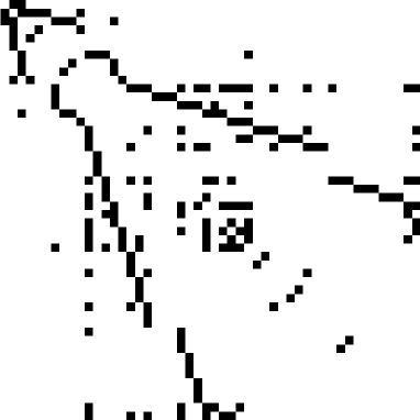
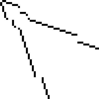
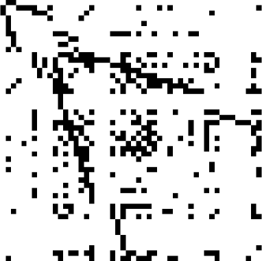
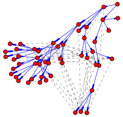
We evaluated the proposed method in two aspects, the reconstruction performance of the recruitment-induced subgraph and the parameter estimation of the edgewise inter-recruitment time model. Let $\mathbf{A}$ be the adjacency matrix of the true recruitment-induced subgraph $G_{S}$ and $\hat{\mathbf{A}}$ be the estimate. We define the true and false positive rates (TPR and FPR) as $\mathrm{TPR}(\hat{\mathbf{A}},\mathbf{A})=\sum_{i<j}1\{\hat{\mathbf{A}}_{ij}=1\mbox{ and }\mathbf{A}_{ij}=1\}/\binom{n}{2}$ and $\mathrm{FPR}(\hat{\mathbf{A}},\mathbf{A})=\sum_{i<j}1\{\hat{\mathbf{A}}_{ij}=1\mbox{ and }\mathbf{A}_{ij}=0\}/\binom{n}{2}.$ Fig. 1 illustrates an example of the reconstruction procedure. We simulated a RDS process over the Project 90 graph (?) with power-law edgewise inter-recruitment time distribution, whose shape parameter $\alpha=2$ and scale parameter $x_{\mathrm{min}}=0.5.$ Fifty subjects are recruited in this process. We show clockwise from top left: the true recruitment-induced subgraph $G_{S}$, the observed recruitment graph $G_{R}$, the estimated network with recruitments as blue arrows and dashed lines as inferred edges, and the estimated recruitment-induced subgraph $\hat{G}_{S}$. The TPR equals $0.769$ and the FPR equals $0.106$. The estimated parameter $\hat{\alpha}=1.95$ and $\hat{x}_{\mathrm{min}}=0.49$.

Reconstruction Performance

Refer to caption
Figure 2: True and false positive rates of the reconstruction results for $\mathrm{Gamma}(\alpha,\alpha)$ datasets. Each point corresponds to the reconstruction result of one dataset. The different shapes of the points indicate different shape parameters.
Refer to caption
Figure 3: Difference between true and false positive rates (green and red boxplots, respectively) under the exponential model and the true Gamma model (the vertical axis) with the true shape parameter $\alpha$ (the horizontal axis).
Refer to caption
Figure 4: Distribution of bias in the estimated shape parameter $\hat{\alpha}$ given the estimated adjacency matrix (red boxes) and the true adjacency matrix (green boxes). The horizontal axis represents the values of the true shape parameter $\alpha$. Whisker lengths are $1.5$ times the inter-quartile range.

Impact of distribution parameter

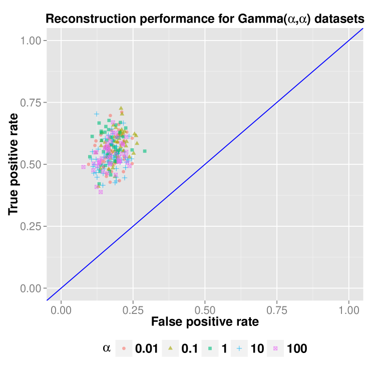
We simulated 50 RDS over the Project 90 graph with inter-recruitment time distribution $\textrm{Gamma}(\alpha,\alpha)$ (parametrized by the shape and scale) for each $\alpha=0.01$, $0.1$, $1,$ $10,$ and $100$. Thus a total number of 250 RDS processes are simulated and the mean inter-recruitment time is fixed to be $1$. The reconstruction performance is illustrated in Fig. 2. Each point on the receiver operating characteristic (ROC) plane represents a reconstruction accuracy performance of a simulated RDS process. Points with the same marker have the same inter-recruitment time distribution parameter. From the figure, we can observe that there is no significant sign of separation of points with different inter-recruitment time distribution parameters. Reconstruction accuracy is robust to the distribution parameter.

Impact of distribution model

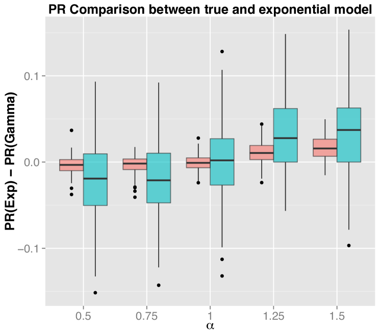
We simulated 50 RDS process over the Project 90 graph with inter-recruitment time distribution $\textrm{Gamma}(0.5,0.5)$. The recruitment-induced subgraph is reconstructed via the model of the true inter-recruitment distribution $\textrm{Gamma}(0.5,0.5)$ and the exponential distribution $\textrm{Exp}(1)$, respectively. The TPR and FPR of each dataset are presented in Fig. 3. The TPR is always higher than the FPR, which reaffirms the effectiveness of our proposed reconstruction method. For each dataset, the TPR and FPR under the true and the exponential models are very close to each other. We observe that there is no significant reconstruction skewness incurred by mis-specification of the inter-recruitment time distribution model.

Parameter Estimation

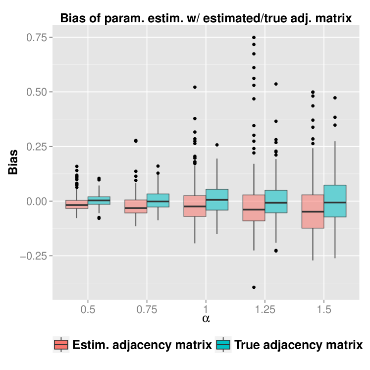
We simulated 200 RDS processes over the Project 90 graph with edgewise inter-recruitment time distribution $\textrm{Gamma}(\alpha,\alpha)$ (parametrized by the shape and scale parameters) for each $\alpha=0.5$, $0.75$, $1,$ $1.25,$ and $1.5$. We used the method in the “Estimation of distribution parameter” section. We assess the bias of the estimated shape parameter $\hat{\alpha}$, which is given by $\hat{\alpha}-\alpha$. Fig. 4 shows the distribution of the bias using Tukey boxplots. In Fig. 4, the red boxes depict the distribution of the biases of the estimated shape parameters inferred through the estimated adjacency matrix, while the green boxes illustrate the distribution of those inferred given the true adjacency matrix. The horizontal axis shows the value of the true shape parameter.

With respect to the red boxes (those based on the estimated adjacency matrices), The middle line of each box is very close to zero and thus the estimation is highly accurate. The interquartile range (IQR) , which measures the deviation of the biases, declines as the shape parameter decreases. Even for the box with largest deviation (i.e., the box with $\alpha=1.5$), the IQR is approximately $[-0.125,0.02]$ and $99.3\%$ of the biases reside in the interval $[-0.27,0.25]$. Compared with the parameter estimation via the true adjacency matrix, this estimator based on the estimated adjacency matrix is biased to some degree. In Fig. 4, we can observe that it underestimates $\alpha$.

Then consider the green boxes (those based on the true adjacency matrix). Similar to those based on the estimated adjacency matrix, the deviation of this estimator declines as the value of the shape parameter $\alpha$ decreases. The middle line of each box is noted to coincide perfectly with zero bias line, which suggests that this estimator is unbiased given the true adjacency matrix.

Experiments on Real Data

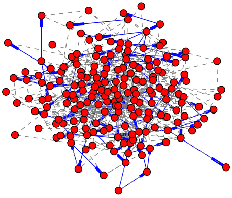
We also apply Render to data from an RDS study of $n=813$ drug users in St. Petersburg, Russian Federation. We use Render to infer the underlying social network structure of the drug users in this study. Since it could be confusing to visualize the whole inferred network, we only show the inferred subgraph of the largest community of the network, as presented in Fig. 5. The blue arrows represent the edges in the recruitment subgraph that indicates the recruiter and recruitee. Gray dashed edges are inferred from the data.

Conclusion

In this paper, we precisely formulated the dynamics of RDS as a continuous-time diffusion process over the underlying graph. We derived the likelihood for the recruitment time series under an arbitrarily recruitment time distribution. As a result, we develop an efficient stochastic optimization algorithm, Render, that identifies the optimum network that best explains the collected data. We then supported the performance of Render through an exhaustive set of experiments on both synthetic and real data.

Acknowledgements

FWC was supported by NIH/NCATS grant KL2 TR000140 and NIMH grant P30MH062294. LC would like to thank Zeya Zhang and Yukun Sun for their encouragement.

Refer to caption
Figure 5: Illustration of the largest community of the inferred underlying social network of the St. Petersburg dataset. The blue arrows represent the edges in the recruitment subgraph that indicates the recruiter and recruitee. Gray dashed edges are inferred from the data.

References

  • [Chen, Crawford, and Karbasi 2015] Chen, L.; Crawford, F. W.; and Karbasi, A. 2015. Seeing the unseen network: Inferring hidden social ties from respondent-driven sampling. arXiv preprint arXiv:1511.04137.
  • [Crawford 2016] Crawford, F. W. 2016. The graphical structure of respondent-driven sampling. Sociological Methodology to appear.
  • [Gile and Handcock 2010] Gile, K. J., and Handcock, M. S. 2010. Respondent-driven sampling: An assessment of current methodology. Sociological Methodology 40(1):285–327.
  • [Goel and Salganik 2009] Goel, S., and Salganik, M. J. 2009. Respondent-driven sampling as Markov chain Monte Carlo. Statistics in Medicine 28(17):2202–2229.
  • [Gomez Rodriguez et al. 2011] Gomez Rodriguez, M.; Balduzzi, D.; Schölkopf, B.; Scheffer, G. T.; et al. 2011. Uncovering the temporal dynamics of diffusion networks. In 28th International Conference on Machine Learning (ICML 2011), 561–568. International Machine Learning Society.
  • [Gomez Rodriguez, Leskovec, and Krause 2010] Gomez Rodriguez, M.; Leskovec, J.; and Krause, A. 2010. Inferring networks of diffusion and influence. In Proceedings of the 16th ACM SIGKDD international conference on Knowledge discovery and data mining, 1019–1028. ACM.
  • [Heckathorn 1997] Heckathorn, D. D. 1997. Respondent-driven sampling: a new approach to the study of hidden populations. SOCIAL PROBLEMS-NEW YORK- 44:174–199.
  • [Heckathorn 2002] Heckathorn, D. D. 2002. Respondent-driven sampling II: deriving valid population estimates from chain-referral samples of hidden populations. Social Problems 49(1):11–34.
  • [Kramer et al. 2009] Kramer, M. A.; Eden, U. T.; Cash, S. S.; and Kolaczyk, E. D. 2009. Network inference with confidence from multivariate time series. Physical Review E 79(6):061916.
  • [Liben-Nowell and Kleinberg 2007] Liben-Nowell, D., and Kleinberg, J. 2007. The link-prediction problem for social networks. Journal of the American society for information science and technology 58(7):1019–1031.
  • [Linderman and Adams 2014] Linderman, S., and Adams, R. 2014. Discovering latent network structure in point process data. In Proceedings of The 31st International Conference on Machine Learning, 1413–1421.
  • [Salganik and Heckathorn 2004] Salganik, M. J., and Heckathorn, D. D. 2004. Sampling and estimation in hidden populations using respondent-driven sampling. Sociological Methodology 34(1):193–240.
  • [Salganik 2006] Salganik, M. J. 2006. Variance estimation, design effects, and sample size calculations for respondent-driven sampling. Journal of Urban Health 83(1):98–112.
  • [Shandilya and Timme 2011] Shandilya, S. G., and Timme, M. 2011. Inferring network topology from complex dynamics. New Journal of Physics 13(1):013004.
  • [Volz and Heckathorn 2008] Volz, E., and Heckathorn, D. D. 2008. Probability based estimation theory for respondent driven sampling. Journal of Official Statistics 24(1):79.
  • [Woodhouse et al. 1994] Woodhouse, D. E.; Rothenberg, R. B.; Potterat, J. J.; Darrow, W. W.; Muth, S. Q.; Klovdahl, A. S.; Zimmerman, H. P.; Rogers, H. L.; Maldonado, T. S.; Muth, J. B.; et al. 1994. Mapping a social network of heterosexuals at high risk for HIV infection. Aids 8(9):1331–1336.

Appendix

Proof of Theorem 1

Proof.

(1) We consider the recruitment of subject $i$. Let $R_{u}(i)$ be the set of recruiters of subject $u$ just before time $t_{i}$ and $I_{u}(i)$ be the set of recruitees of recruiter $u$ just before time $t_{i}$. Suppose that $i\notin M$. The inter-recruitment time between $i$ and its potential recruiter $u$ is denoted $W_{ui}=t_{i}-t_{u}$ and is greater than $t_{i-1}-t_{u}$ conditional on previous recruitment of $i$. Let $U$ be the random variable of next recruiter and $X$ be the random variable of next recruitee. Let $J$ denote the event $\forall j\in R(i),k\in I(i),W_{jk}>t_{i-1}-t_{j}$. We have

$\displaystyle\operatorname{Pr}\left[U=u,X=x,W_{ux}\geq t-t_{u}\mid J\right]$
$\displaystyle=$ $\displaystyle\operatorname{Pr}\left[W_{ux}\geq t-t_{u},t_{j}+W_{jk}>t_{u}+W_{ux},\right.$
$\displaystyle\left.\forall j\in R(i),k\in I(i),\{u,x\}\neq\{j,k\}\mid J\right],$

and

$\displaystyle\operatorname{Pr}\left[W_{Ui}\geq t-t_{U}\mid J\right]$
$\displaystyle=$ $\displaystyle\sum_{x\in I(i)}\sum_{u\in R_{x}(i)}\operatorname{Pr}\left[W_{ux}\geq t-t_{u},t_{j}+W_{jk}>t_{u}\right.$
$\displaystyle\left.+W_{ux},\forall j\in R(i),k\in I(i),\{u,x\}\neq\{j,k\}\mid J\right]$
$\displaystyle=$ $\displaystyle\sum_{x\in I(i)}\sum_{u\in R_{x}(i)}\int_{t-t_{u}}^{\infty}f_{\tau(u;i)}(s)\mathrm{d}s\operatorname{Pr}\left[W_{jk}>s+t_{u}\right.$
$\displaystyle\left.-t_{j},\forall j\in R(i),k\in I(i),\{u,x\}\neq\{j,k\}\mid J\right]$
$\displaystyle=$ $\displaystyle\sum_{x\in I(i)}\sum_{u\in R_{x}(i)}\int_{t-t_{u}}^{\infty}f_{\tau(u;i)}(s)\cdot$
$\displaystyle\frac{\prod_{j\in R(i)}\prod_{k\in I_{j}(i)}\left(1-F_{\tau(j;i)}(s+t_{u}-t_{j})\right)}{1-F_{\tau(u;i)}(s)}\mathrm{d}s$
$\displaystyle=$ $\displaystyle\sum_{x\in I(i)}\sum_{u\in R_{x}(i)}\int_{t-t_{u}}^{\infty}H_{\tau(u;i)}(s)\cdot$
$\displaystyle\prod_{j\in R(i)}S_{\tau(j;i)}^{|I_{j}(i)|}(s+t_{u}-t_{j})\mathrm{d}s$

Thus the likelihood is

$\displaystyle\sum_{x\in I(i)}\sum_{u\in R_{x}(i)}H_{\tau(u;i)}(t_{i}-t_{u})\prod_{j\in R(i)}S_{\tau(j;i)}^{|I_{j}(i)|}(t_{i}-t_{j})$
$\displaystyle=$ $\displaystyle\prod_{j\in R(i)}S_{\tau(j;i)}^{|I_{j}(i)|}(t_{i}-t_{j})\sum_{u\in R(i)}|I_{u}(i)|H_{\tau(u;i)}(t_{i}-t_{u})$

Now suppose that $i\in M$.

$\displaystyle\operatorname{Pr}\left[W_{jk}\geq t-t_{j},\forall j\in R(i),k\in I_{j}(i)\mid J\right]$
$\displaystyle=$ $\displaystyle\prod_{j\in R(i)}\prod_{k\in I_{j}(i)}(1-F_{\tau(j;i)}(t-t_{j}))$
$\displaystyle=$ $\displaystyle\prod_{j\in R(i)}S_{\tau(j;i)}^{|I_{j}(i)|}(t-t_{j}).$

Thus the likelihood is

$$\prod_{j\in R(i)}S_{\tau(j;i)}^{|I_{j}(i)|}(t_{i}-t_{j}).$$

Therefore the entire likelihood is

$$\prod_{i=1}^{n}\left(\sum_{u\in R(i)}|I_{u}(i)|H_{\tau(u;i)}(t_{i}-t_{u})\right)^{1\{i\notin M\}}\cdot\\ \prod_{j\in R(i)}S_{\tau(j;i)}^{|I_{j}|}(t_{i}-t_{j}).$$

(2) The log-likelihood is

$$\sum_{i=1}^{n}\left[1\{i\notin M\}\log\left(\sum_{u\in R(i)}|I_{u}(i)|H_{\tau(u;i)}(t_{i}-t_{u})\right)\right.\\ \left.+\sum_{j\in R(i)}|I_{j}(i)|\log S_{\tau(j;i)}(t_{i}-t_{j})\right].$$

And the number of recruitees of recruiter $u$ just before time $t_{i}$ is given by

$$|I_{j}(i)|=\mathbf{C}_{ji}\left(\sum_{k=i}^{n}\mathbf{A}_{jk}+\mathbf{u}_{j}\right).$$

The term $\sum_{u\in R(i)}|I_{u}(i)|H_{\tau(u;i)}(t_{i}-t_{u})$ in the log-likelihood is given by

$\displaystyle\sum_{u\in R(i)}|I_{u}(i)|H_{\tau(u;i)}(t_{i}-t_{u})$
$\displaystyle=$ $\displaystyle\sum_{u}\mathbf{C}_{ui}\left(\sum_{k=i}^{n}\mathbf{A}_{uk}+\mathbf{u}_{u}\right)\mathbf{H}_{ui}$
$\displaystyle=$ $\displaystyle(\mathbf{B}^{\prime}\mathbf{u}+\operatorname{LowerTri}(\mathbf{A}\mathbf{B})^{\prime}\cdot\mathbf{1})_{i}.$

The term $\sum_{j\in R(i)}|I_{j}(i)|\log S_{\tau(j;i)}(t_{i}-t_{j})$ in the log-likelihood is given by

$\displaystyle\sum_{j\in R(i)}|I_{j}(i)|\log S_{\tau(j;i)}(t_{i}-t_{j})$
$\displaystyle=$ $\displaystyle\sum_{j\in R(i)}\mathbf{C}_{ji}\left(\sum_{k=i}^{n}\mathbf{A}_{jk}+\mathbf{u}_{j}\right)\mathbf{S}_{ji}$
$\displaystyle=$ $\displaystyle(\mathbf{D}^{\prime}\mathbf{u}+\operatorname{LowerTri}(\mathbf{A}\mathbf{D})^{\prime}\cdot\mathbf{1})_{i}.$

Thus the log-likelihood is

$$\sum_{i=1}^{n}\left[1\{i\notin M\}\log\left(\mathbf{B}^{\prime}\mathbf{u}+\operatorname{LowerTri}(\mathbf{A}\mathbf{B})^{\prime}\cdot\mathbf{1}\right)_{i}\right.\\ \left.+\left(\mathbf{D}^{\prime}\mathbf{u}+\operatorname{LowerTri}(\mathbf{A}\mathbf{D})^{\prime}\cdot\mathbf{1}\right)_{i}\right]=\mathbf{m}^{\prime}\beta+\mathbf{1}^{\prime}\delta.$$

Proof of connectedness of the space of compatible adjacency matrices

Proof.

Consider two compatible adjacency matrices $\mathbf{A}_{1}$ and $\mathbf{A}_{2}$. Their Hadamard product $\mathbf{A}_{1}\circ\mathbf{A}_{2}$, which corresponds to the maximum common subgraph of $\mathbf{A}_{1}$ and $\mathbf{A}_{2}$, is also compatible. We can remove the edges in $\mathbf{A}_{1}$ that do not appear in $\mathbf{A}_{1}\circ\mathbf{A}_{2}$ one at a time, and thus arrive at state $\mathbf{A}_{1}\circ\mathbf{A}_{2}$. Then we add the edges in $\mathbf{A}_{2}$ that do not appear in $\mathbf{A}_{1}\circ\mathbf{A}_{2}$ once at a time, and thus finally arrive at state $\mathbf{A}_{2}$. All intermediate adjacency matrices in this procedure are compatible. ∎

Proof of Theorem 2

Proof.

In fact, the total number of possible edges that can be added for $\mathbf{A}(\jmath)$ is given by $\mathrm{Add}(\mathbf{A}(\jmath))$ and the total number of possible edges that can be removed for $\mathbf{A}(\jmath)$ is given by $\mathrm{Remove}(\mathbf{A}(\jmath))$. Thus we have the proposal distribution

$$\operatorname{Pr}(\tilde{\mathbf{A}}(\jmath+1)|\mathbf{A}(\jmath))=\frac{1}{\mathrm{Add}(\mathbf{A}(\jmath))+\mathrm{Remove}(\mathbf{A}(\jmath))}.$$

Similarly, we have

$$\operatorname{Pr}(\mathbf{A}(\jmath)|\tilde{\mathbf{A}}(\jmath+1))=\\ \frac{1}{\mathrm{Add}(\tilde{\mathbf{A}}(\jmath+1))+\mathrm{Remove}(\tilde{\mathbf{A}}(\jmath+1))}.$$ (2)

Thus we obtain the proposal ratio:

$$\frac{\operatorname{Pr}(\mathbf{A}(\jmath)|\tilde{\mathbf{A}}(\jmath+1))}{\operatorname{Pr}(\tilde{\mathbf{A}}(\jmath+1)|\mathbf{A}(\jmath))}\\ =\frac{1/\text{$\left(\mathrm{Add}(\tilde{\mathbf{A}}(\jmath+1))+\mathrm{Remove}(\tilde{\mathbf{A}}(\jmath+1))\right)$}}{1/\left(\mathrm{Add}(\mathbf{A}(\jmath))+\mathrm{Remove}(\mathbf{A}(\jmath))\right)}\\ =\frac{\mathrm{Add}(\mathbf{A}(\jmath))+\mathrm{Remove}(\mathbf{A}(\jmath))}{\mathrm{Add}(\tilde{\mathbf{A}}(\jmath+1))+\mathrm{Remove}(\tilde{\mathbf{A}}(\jmath+1))}.$$

Proof of Theorem 3

Proof.

Let $\mathbf{J}^{ab}$ denote the $n\times n$ matrix whose $(a,b)$-entry is one and all other entries are zeros. We have

$$\tilde{\mathbf{A}}(\jmath+1)-\mathbf{A}(\jmath)=\pm\left(\mathbf{J}^{ab}+\mathbf{J}^{ba}\right),$$

where we assign the minus sign “$-$” in “$\pm$” if the edge that connects subjects $a$ and $b$ is added to $\tilde{\mathbf{A}}(\jmath+1)$ and we assign the plus sign “$+$” in “$\pm$” if that edge is removed from $\mathbf{A}(\jmath)$. And $e^{\beta(\mathbf{A})}$ can be re-written as

$\displaystyle e^{\beta(\mathbf{A})}$
$\displaystyle=$ $\displaystyle\mathbf{B}^{\prime}\mathbf{u}+\operatorname{LowerTri}(\mathbf{A}\mathbf{B})^{\prime}\cdot\mathbf{1}$
$\displaystyle=$ $\displaystyle\mathbf{B}^{\prime}(\mathbf{d}-\mathbf{A}\cdot\mathbf{1})+\operatorname{LowerTri}(\mathbf{A}\mathbf{B})^{\prime}\cdot\mathbf{1}$
$\displaystyle=$ $\displaystyle\mathbf{B}^{\prime}\mathbf{d}-\mathbf{B}^{\prime}\mathbf{A}\cdot 1+\operatorname{LowerTri}(\mathbf{A}\mathbf{B})^{\prime}\cdot\mathbf{1}$
$\displaystyle=$ $\displaystyle\mathbf{B}^{\prime}\mathbf{d}-\mathbf{B}^{\prime}\mathbf{A}^{\prime}\cdot 1+\operatorname{LowerTri}(\mathbf{A}\mathbf{B})^{\prime}\cdot\mathbf{1}$ (3)
$\displaystyle=$ $\displaystyle\mathbf{B}^{\prime}\mathbf{d}-(\mathbf{A}\mathbf{B})^{\prime}\cdot 1+\operatorname{LowerTri}(\mathbf{A}\mathbf{B})^{\prime}\cdot\mathbf{1}$
$\displaystyle=$ $\displaystyle\mathbf{B}^{\prime}\mathbf{d}-\operatorname{StrictlyUpperTri}(\mathbf{A}\mathbf{B})^{\prime}\cdot\mathbf{1},$

where in (3) we use the fact that $\mathbf{A}$ is symmetric and $\operatorname{StrictlyUpperTri}(\cdot)$ denotes the strictly upper triangular part (diagonal entries exclusive) of a matrix. Thus

$$e^{\beta(\mathbf{A})\pm\mathbf{J}^{ab}}-e^{\beta(\mathbf{A})}=\pm\operatorname{StrictlyUpperTri}(\mathbf{J}^{ab}\mathbf{B})^{\prime}\cdot\mathbf{1}.$$

The $(i,j)$-entry of $\mathbf{J}^{ab}\mathbf{B}$ is

$\displaystyle(\mathbf{J}^{ab}\mathbf{B})_{ij}$
$\displaystyle=$ $\displaystyle\sum_{k=1}^{n}\mathbf{J}_{ik}^{ab}\mathbf{B}_{kj}$
$\displaystyle=$ $\displaystyle\mathbf{J}_{ib}^{ab}\mathbf{B}_{bj}.$

Thus

$\displaystyle\left(\operatorname{StrictlyUpperTri}(\mathbf{J}^{ab}\mathbf{B})^{\prime}\cdot\mathbf{1}\right)_{j}$
$\displaystyle=$ $\displaystyle\sum_{i:i<j}\mathbf{J}_{ib}^{ab}\mathbf{B}_{bj}$
$\displaystyle=$ $\displaystyle\mathbf{B}_{bj}1\{a<j\}.$

Hence we have

$$(e^{\beta(\tilde{\mathbf{A}}(\jmath+1))}-e^{\beta(\mathbf{A}(\jmath))})_{j}\\ =\pm\left(\mathbf{B}_{bj}1\{a<j\}-\mathbf{B}_{aj}1\{b<j\}\right).$$ (4)

Similarly, if we view $\delta$ in Theorem 1 as a function of the adjacency matrix $\mathbf{A}$, denoted by $\delta(\mathbf{A})$, we have

$$\delta(\tilde{\mathbf{A}}(\jmath+1))-\delta(\beta(\mathbf{A}(\jmath)))\\ =\pm\left(\mathbf{D}_{bj}1\{a<j\}-\mathbf{D}_{aj}1\{b<j\}\right).$$ (5)

If we plug in Equations (4) and (5) in the likelihood ratio $\frac{\Lambda_{\gamma_{\jmath}}(\tilde{\mathbf{A}}(\jmath+1);{\mathbf{t},\hat{\theta}_{\iota})}}{\Lambda_{\gamma_{\jmath}}(\mathbf{A}(\jmath);\mathbf{t},\hat{\theta}_{\iota})}$, we obtain the expression in the theorem statement.∎