Sequence to Sequence Learning for Optical Character Recognition

Abstract

We propose an end-to-end recurrent encoder-decoder based sequence learning approach for printed text Optical Character Recognition (ocr). In contrast to present day existing state-of-art ocr solution [Graves et al. (2006)] which uses ctc output layer, our approach makes minimalistic assumptions on the structure and length of the sequence. We use a two step encoder-decoder approach – (a) A recurrent encoder reads a variable length printed text word image and encodes it to a fixed dimensional embedding. (b) This fixed dimensional embedding is subsequently comprehended by decoder structure which converts it into a variable length text output. Our architecture gives competitive performance relative to Connectionist Temporal Classification (ctc) [Graves et al. (2006)] output layer while being executed in more natural settings. The learnt deep word image embedding from encoder can be used for printed text based retrieval systems. The expressive fixed dimensional embedding for any variable length input expedites the task of retrieval and makes it more efficient which is not possible with other recurrent neural network architectures. We empirically investigate the expressiveness and the learnability of long short term memory (lstms) in the sequence to sequence learning regime by training our network for prediction tasks in segmentation free printed text ocrs. The utility of the proposed architecture for printed text is demonstrated by quantitative and qualitative evaluation of two tasks – word prediction and retrieval.

1 Introduction

Deep Neural Nets (dnns) have become present day de-facto standard for any modern machine learning task. The flexibility and power of such structures have made them outperform other methods in solving some really complex problems of speech [Hinton et al. (2012)] and object [Krizhevsky et al. (2012)] recognition. We exploit the power of such structures in an ocr based application for word prediction and retrieval with a single model. Optical character recognition (ocr) is the task of converting images of typed, handwritten or printed text into machine-encoded text. It is a method of digitizing printed texts so that it can be electronically edited, searched, stored more compactly, displayed on-line and used in machine processes such as machine translation, text-to-speech and text mining.

From character recognition to word prediction, ocrs in recent years have gained much awaited traction in mainstream applications. With its usage spanning across handwriting recognition, print text identification, language identification etc. ocrs have humongous untapped potential. In our present work we show an end-to-end, deep neural net, based architecture for word prediction and retrieval. We conceptualize the problem as that of a sequence to sequence learning and use rnn based architecture to first encode input to a fixed dimension feature and later decode it to variable length output. Recurrent Neural Networks (rnn) architecture has an innate ability to learn data with sequential or temporal structure. This makes them suitable for our application. Encoder lstm network reads the input sequence one step at a time and converts it to an expressive fixed-dimensional vector representation. Decoder lstm network in turn converts this fixed-dimensional vector (Figure 1(b)) to the text output.

Encoder-Decoder framework has been applied to many applications recently. [Sutskever et al. (2011)] used recurrent encoder-decoder for character-level language modelling task where they predict the next character given the past predictions. It has also been used for language translation [Sutskever et al. (2014)] where a complete sentence is given as input in one language and the decoder predicts a complete sentence in another language. Vinyals et al. [Vinyals et al. (2014)] presented a model based on a deep recurrent architecture to generate natural sentences describing an image. They used a convolutional neural network as encoder and a recurrent decoder to describe images in natural language. Zaremba et al. [Zaremba & Sutskever (2014)] used sequence to sequence learning for evaluating short computer programs, a domain that have been seen as too complex in past. Vinyals et al. [Vinyals & Le (2015)] proposed neural conversational networks based of sequence to sequence learning framework which converses by predicting the next sentence given the previous sentence(s) in a conversation. In the same spirit as Vinyals et al. (2014); Sutskever et al. (2014), we formulate the ocr problem as a sequence to sequence mapping problem to convert an input (text) image to its corresponding text.

In this paper, we investigate the expressiveness and learnability of lstms in sequence to sequence learning regime for printed text ocr. We demonstrate that sequence to sequence learning is suitable for word prediction task in a segmentation free setting. We even show the expressiveness of the learnt deep word image embeddings (from Encoder network of prediction) on image retrieval task. In (majority of) cases where standard lstm models do not convert a variable length input to a fixed dimensional output, we are required to use Dynamic Time Warping (dtw) for retrieval which tends to be computationally expensive and slow. Converting variable length samples to fixed dimensional representation gives us access to fast and efficient methods for retrieval in fixed dimensional regime –- approximate nearest neighbour.

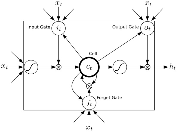
(a) LSTM block

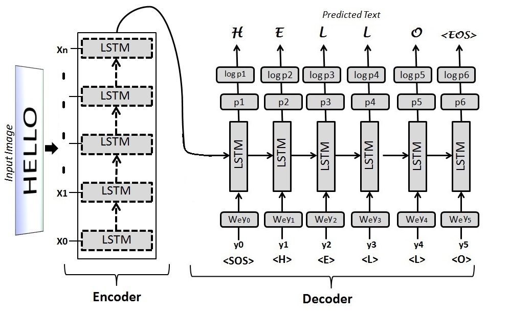
(b) Encoder Decoder Framerwork for OCR

Figure 1: Figure 1(a) is the lstm block comprised of input, output and forget gates. Figure 1(b) showcases the proposed recurrent encoder decoder framework for Optical Character Recognition. The Encoder lstm section reads the input image and converts it to a fixed-dimensional vector representation. Decoder lstm in turn generates the text output corresponding to fixed-dimensional vector representation.

2 Sequence learning

A recurrent neural network (rnn) is a neural network with cyclic connections between its units. These cycles create a concept of ‘internal memory’ in network and thus differentiate rnns from other feed forward networks. The internal memory of rnn can be used to process arbitrary sequences of inputs – given a variable length input sequence $X$ we can generate corresponding variable length output sequence $Y$. This is done by sequentially reading each time-step $x_{t}$ of input sequence $X$ and updating its internal hidden representations $h_{t}$. More sophisticated recurrent activation functions like lstm [Hochreiter & Schmidhuber (1997)] and gru [Cho et al. (2014); Chung et al. (2014)] have become more common in recent days. They perform better when compared to other vanilla rnn implementations.

Long Short-Term Memory [Hochreiter & Schmidhuber (1997)] is a rnn architecture that elegantly addresses the vanishing gradients problem using ‘memory units’. These linear units have a pair of auxiliary ‘gating units’ that control the flow of information to and from the unit. Equations 1-5 describe lstm blocks.

$$i_{t} =\sigma(W_{xi}x_{t}+W_{hi}h_{t-1}+w_{ci}\odot c_{t-1}+b_{i})$$ (1)

$$f_{t} =\sigma(W_{xf}x_{t}+W_{hf}h_{t-1}+w_{cf}\odot c_{t-1}+b_{f})$$ (2)

$$c_{t} =f_{t}c_{t-1}+i_{t}tanh(W_{xc}x_{t}+W_{hc}h_{t-1}+b_{c})$$ (3)

$$o_{t} =\sigma(W_{xo}x_{t}+W_{ho}h_{t-1}+w_{co}\odot c_{t-1}+b_{o})$$ (4)

$$h_{t} =o_{t}tanh(c_{t})$$ (5)

Here, $W_{xi},W_{hi},w_{ci},b_{i}$ are input gate parameters. $W_{xo},W_{ho},w_{co},b_{o}$ are output gate parameters. $W_{xf},W_{hf},w_{cf},b_{f}$ are forget gate parameters. $W_{xc},W_{hc},b_{c}$ are parameters associated with input which directly modify the memory cells. The symbol $\odot$ denotes element-wise multiplication. The gating units are implemented by multiplication, so it is natural to restrict their domain to $[0,1]^{N}$, which corresponds to the sigmoid non-linearity. The other units do not have this restriction, so the tanh non-linearity is more appropriate. We use collection of such units (Figure  1(a)) to describe an encoder-decoder framework for the ocr task. We formulate the task of ocr prediction as a mapping problem between structured input (image) and structured output (text).

Let, $\{I_{i},Y_{i}\}_{i=1}^{N}$ define our dataset with $I_{i}$ being image and $Y_{i}$ be the corresponding text label. Image $I_{i}$ lies in $\mathbb{R}^{H\times T_{i}}$, where $H$ is word image height (common for all images) and $T_{i}$ is the width of $i^{th}$ word image. We represent both image and label as a sequence – Image $I_{i}=\{x_{1},x_{2},...,x_{T_{i}}\}$ is sequence of $T_{i}$ vectors lying in $\{0,1\}^{H}$ ($x_{i}$ is a $i_{th}$ pixel column) and $Y_{i}=\{y_{1},y_{2},...,y_{M_{i}}\}$ is corresponding label which is a sequence of $M_{i}$ unicode characters. We learn a mapping from image to text in two steps – (a) $f_{encoder}:I_{i}\rightarrow z_{i}$, maps an image $I_{i}$ to a latent fixed dimensional representation $z_{i}$ (b) $f_{decoder}:z_{i}\rightarrow Y_{i}$ maps it to the output text sequence $Y_{i}$. Unlike ctc layer based sequence prediction [Graves et al. (2006)] we don’t have any constraint on length of sequences $I_{i}$ and $Y_{i}$. Equations 6-7 formally describe the idea. The choice of $f_{encoder}$ and $f_{decoder}$ depends on type of input and output respectively. Both input and output correspond to a sequence in our case, hence we use recurrent encoder and recurrent decoder formulation.

$$z_{i} =f_{encoder}(I_{i})$$ (6)

$$P(Y_{i}|I_{i}) =f_{decoder}(z_{i})$$ (7)

2.1 Encoder: lstm based Word Image Reader

To describe the formulation we use vanilla rnns with $L$ hidden layer and no output layer. The encoder reads $I_{i}=\{x_{1},x_{2},...,x_{T_{i}}\}$ one step at a time from $x_{1}$ to $x_{T_{i}}$. Hidden state $h^{n}_{t}$ is updated using equations 8-9 using current input $x_{t}$ and previous hidden state $\{h^{n}_{t-1}\}_{n=1}^{L}$ where $L$ is the number of hidden layers in rnn.

$$h^{1}_{t} =relu(W_{ih^{1}}x_{t}+W_{h^{1}h^{1}}h^{1}_{t-1}+b_{h}^{1})$$ (8)

$$h^{n}_{t} =relu(W_{h^{n-1}h^{n}}h^{n-1}_{t}+W_{h^{n}h^{n}}h^{n}_{t-1}+b_{h}^{n})$$ (9)

where $W_{ih^{1}},W_{h^{1}h^{1}},b_{h}^{1},W_{ih^{n}},W_{h^{n-1}h^{n}},W_{h^{n}h^{n}},b_{h}^{n}$ are parameters to be learned.

To obtain our fixed dimensional latent representation $z_{i}$ we use the final hidden states $\{h^{n}_{T_{i}}\}_{n=1}^{L}$.

$$z_{i} =\{h^{n}_{T_{i}}\}_{n=1}^{L}$$ (10)

It should be noted that we have used lstm networks instead of vanilla rnns and no output layer for encoder is needed. The hidden states of last step $T_{i}$ are used as initial state of decoder network.

2.2 Decoder: lstm based Word Predictor

Similar to encoder, we describe the idea using vanilla rnns with $L$ hidden layers and softmax output layer. The goal of word predictor is to estimate the conditional probability $p(Y_{i}|I_{i})$ as shown in equation 11-12, where $I_{i}$ is image input sequence and $Y_{i}$ is output sequence.

$$p(Y_{i}|I_{i}) =p(Y_{i}=\{y_{1},\ldots,y_{T^{\prime}}\}|I_{i}=\{x_{1},\ldots,x_{T_{i}}\})$$ (11)

$$=\prod_{t=1}^{T^{\prime}}p(y_{t}|I_{i},y_{1},\ldots,y_{t-1})$$ (12)

The updates for single step for rnn is described in equations 13-16. The hidden state $h^{n}_{t}$ is updated using equations 13 - 14 using current input $x_{t}$ and previous hidden state $\{h^{n}_{t-1}\}_{n=1}^{L}$, where $L$ is number of hidden layers in rnn. The hidden activations, $h^{L}_{t-1}$ are used to predict the output at step $t$ using equations 15-16. $x_{t}$ is the embedding of the most probable state in previous step $t-1$ shown in equation 18.

$$h^{1}_{t} =relu(W_{ih^{1}}x_{t}+W_{h^{1}h^{1}}h^{1}_{t-1}+b_{h}^{1})$$ (13)

$$h^{n}_{t} =relu(W_{h^{n-1}h^{n}}h^{n-1}_{t}+W_{h^{n}h^{n}}h^{n}_{t-1}+b_{h}^{n})$$ (14)

$$o_{t} =W_{h^{L}o}h^{L}_{t}+b_{o}$$ (15)

$$p_{t} =sofmax(o_{t})$$ (16)

where $W_{ih^{1}},W_{h^{1}h^{1}},b_{h}^{1},W_{ih^{n}},W_{h^{n-1}h^{n}},W_{h^{n}h^{n}},b_{h}^{n},W_{h^{L}o},b_{o}$ are parameters to be learned.

Decoding begins at $t=0$ with $\langle SOS\rangle$ marker (Start Of Sequence). The state $t=-1$ is initialized with the final state $z_{i}$ of encoder as shown in equation 17. The $1^{st}$ character is predicted using the embedding for $\tilde{y}_{0}=\langle SOS\rangle$ as input $x_{0}=W_{e}\tilde{y}_{0}$ and output $p_{1}(y_{1}|I_{i},y_{0})$ where $W_{e}$ is the embedding matrix for characters. As shown in equation 18, every ${t_{th}}$ character is predicted using the embedding for $\tilde{y}_{t}={\arg\max}~{}p_{t}(y_{t}|I_{i},y_{<t})$ as input and output $p_{t}(y_{t}|I_{i},y_{<t})$. This is iterated till $t=T^{\prime}$ where $y_{T^{\prime}}=\langle EOS\rangle$ (End Of Sequence). $T^{\prime}$ is not known in priori, $\langle EOS\rangle$ marker instantiates the value of $T^{\prime}$.

$$h_{-1} =f_{encoder}(I)$$ (17)

$$x_{t} =W_{e}\tilde{Y}_{t}$$ (18)

$$p_{t+1} =f_{decoder}(x_{t})$$ (19)

$W_{e}$ in equation 18 is the embedding matrix for characters. It should be (again) noted that we use lstm networks (equations 1 - 5) instead of vanilla rnns (equations 13, 14).

2.3 Training

The model described in section 2.1 and 2.2 is trained to predict characters of the input word (image) sequence. The input at time $t$ of decoder is an embedding of the output of time $t-1$. The loss $L$ for a sample $(I,Y)$ is described by equation 20.

$$L(I,Y) =-\log p(Y|I;\theta)$$ (20)

Here, $\log p(Y|I;\theta)=\sum_{t=0}^{M}\log p(y_{t}|I,y_{0},\ldots,y_{t-1};\theta)$ is the $\log$ probability of correct symbol at each step. We search for the parameters $\theta^{*}$ which minimize the expected loss over true distribution $P(I,Y)$ given in equation 21. This distribution is unknown and can be approximated with empirical distribution $\tilde{P}(I,Y)$ given in equation 22-23.

$$\theta^{*} =\underset{\theta}{\arg\min}~{}\mathbb{E}_{P(I,Y)}L(I,Y;\theta)$$ (21)

$$\approx\underset{\theta}{\arg\min}~{}\mathbb{E}_{\tilde{P}(I,Y)}L(I,Y;\theta)$$ (22)

$$=\underset{\theta}{\arg\min}\frac{1}{N}\sum_{i=1}^{N}L(I_{i},Y_{i};\theta)$$ (23)

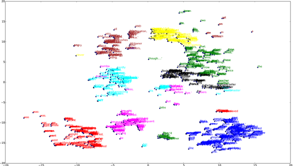
(a) TSNE plots for feature representation of unique words starting with top eight most frequent alphabets(S, T, W, H, B, C, F, A including lowercase. (Color based on first alphabet of words)

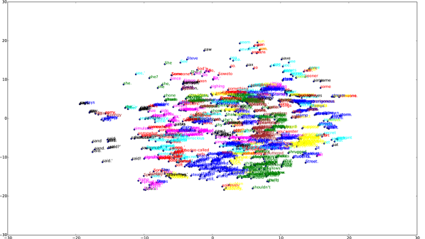
(b) TSNE plots for feature representation of unique words starting with S and top eight second alphabets (t, h, o, e, i, u, a, p) in word with respect to population in S. (Color based on second alphabet of words starting with S.)

Figure 2: tsne plots characterizing the quality of feature representations computed by encoder. Each word has a unique high dimensional feature representation which is then embedded in a two dimensional space (using tsne) and is visualized using scatter plots. Similar words are grouped together (shown with various colours) and dissimilar words tend to get far away. As shown in the figure, (a) words starting with same alphabets belong to same clusters and rest are in other clusters (b) words beginning with ’S’ and having same second alphabet belong to same clusters and rest are in other clusters. (Readers are requested to magnify the graphs to look into the intricate details of clusters)

3 Implementation Details

Keeping the aspect ratio of input images intact we resize them to height of $30$ pixels. The resized binary images are then used as an input to the two layer lstm encoder-decoder architecture. We use embedding size of $25$ for all our experiments. The dimensionality of output layer in decoder is equal to number of unique symbols in the dataset. rms prop [Tieleman & Hinton (2012)] with step size of $0.0001$ and momentum of $0.99$ is used to optimize the loss. All relevant parameters are verified and set using a validation set. We use Python’s numpy library to implement lstm based architecture. The network is built using computational graphs.

4 Experiments

Features	Dim	mAP-100	mAP-5000
bow	400	0.5503	0.33
bow	2000	0.6321	-
Augmented Profiles	247	0.7371	0.6189
lstm-encoder	400	0.7402 $(h1-h2)$	0.8521
		0.8521 $(c1-c2)$
ocr - tesseract	-	0.6594	0.7095
ocr - abbyy	-	0.8583	0.872

Table 1: mAP computed for various methods: mAP-n stands for mean average precision computed over top n retrievals. $hi$ is hidden representation of layer-$i$ at last timestep of input sequence. $ci$ is memory for layer-$i$ at last timestep of input sequence. A-B is the concatenation of representation A and B. For example, $h1-h2$ represents concatenation of both $h1$ and $h2$.

Model Label error(%) abbyy 1.84 tesseract 35.80 tesseract 16.95 rnn Encoder-Decoder 35.57 lstm-ctc [Graves et al. (2006)] 0.84 lstm Encoder-Decoder 0.84

Feature mAP-100 h1-h2 0.7239 c1-c2 0.8548 h1-h2-c1-c2 L1 0.8078 h1-h2-c1-c2 L2 0.7834 h1-h2-c1-c2 0.8545

Table 2: Left: Label Error Rate comparison of rnn-ctc and Recurrent encoder-decoder.Right: Effect of different concatenation and normalization on features from LSTM-Encoder. l1 and l2 represent normalization scheme.

Table 3: Qualitative results for retrieval: Comparison of retrieval scheme using simple Bag of Words (BoW) and proposed Deep Word Image Embeddings (DWIE). We use text labels (to save space and more clarity in presentation) of both query and retrieved images to illustrate difference in performance of two approaches. The proposed approach is far more robust to text variations in images and captures much more intricate details about the images.

	DWIE	BoW	DWIE	BoW	DWIE	BoW	DWIE	BoW
Query ($\rightarrow$) / Retrival ($\downarrow$)	A.	A.	following	following	returned	returned	For	For
R1	A.	”A	following	long	returned	turned	For	For
R2	A.	A	following	long	returned	read	For	For
R3	A.	A	following	long	returned	refused	For	For
R4	A.	At	following	following	returned	retorted	For	For
R5	A.	Ah	following	long	returned	lifted	For	For
R6	A	A	following	flowing	returned	ceased	For	For
R7	A	A	following	long	returned	rolled	For	For
R8	A	A	folding	long	returned	and	For	For
R9	A	A	follow	long	returned	carried	For	for
R10	A	A	followed,	following	returned	red	For	for
R11	A	A	foolishly	long	returned	Head	For	for
R12	A	A	fellow,	along	returned	raised	For	for
R13	A	A	foolscap	long	returned	caused	For	for
R14	A	A	fellow,	following	returned	turned	For	for
R15	A	A	foliage.	long	returned	turned	For	for
R16	A	A	fellow,	long	returned.	road	For	for
R17	A	A	fellow,	long	retired	and	For	for
R18	A	A	fellow,	long	retorted	returned	Fer-	For
R19	A	As	falling	long	return.”	God	Fer-	for
R20	A	Af-	follow,”	closing	return	acted	Fer-	For
# relevant matches in corpus	5	5	7	7	15	15	17	17

We demonstrate the utility of the proposed recurrent encoder-decoder framework by two related but independent tasks. Independent baselines are set for both prediction and retrieval experiments.

Prediction: We use $295$K annotated English word images from seven books for our experiments. We perform three way data split for all our experiments – 60% training, 20% validation and remaining 20% for testing. Results are reported by computing ‘label error rate’. Label error rate is defined as ratio of sum of insertions, deletions and substitutions relative to length of ground truth over dataset. We compare the results of our pipeline with state-of-art lstm-ctc [Graves et al. (2006)], an open-source ocr tesseract [tes ] and a commercial ocr abbyy [abb ].

Retrieval: We use $108$K annotated word images from book titled ‘Adventures of Sherlock Holmes’ for retrieval experiments. In all $43$K word images are used for querying the retrieval system. We compare retrieval results with SIFT [Lowe (2004)] based bag of words representation, augmented profiles [Kumar et al. (2007)] and commercial [ocr abbyy].

Table 4: Qualitative results for prediction: We illustrate some of the success and failure cases of our word prediction output. The figure highlights the cases where both commercial and open-source ocrs fail

Query Image($\rightarrow$)
True Label	mom	OK,’	jump	go.’
Tessaract	IDOITI	ox,’	iump	80.
Abbyy	UJOUJ	ok;	duinl	g -’
LSTM-ED	mom	OK,’	jump	go.’

4.1 Results and Discussion

Table 2 exhibits prediction baseline. We observe that lstm Encoder-Decoder outperforms vanilla rnn Encoder-Decoder by significant margin. It even scores better when compared to lstm with ctc output layer and abbyy. When compared to ctc layer based lstm networks, our network requires more memory space. The strength of our network is fixed length representation for variable length input which enables us to perform better and faster retrieval.

Table 1 depicts retrieval baseline. Features from lstm encoder (referred as deep word image embedding (dwie)) are used for comparisons with other state-of-art results. We observe that dwie features significantly outperform sift [Lowe (2004)] based bag of words (bow) and augmented profiles [Kumar et al. (2007)]. When compared to abbyy, dwie features perform a notch better for top $5000$ retrieval but perform similar for top $100$ retrieval. The memory states at last position of each sequence are used as dwie features. Various normalization (L1 and L2) and augmentations with hidden states were tried out as shown in Table 2.

Table 3 demonstrates the qualitative performance of retrieval system using both deep word image embedding (dwie) and bag of words (bow) models. The table illustrates top $20$ retrievals using both the methods. We observe the proposed embeddings to be better than naive (bow) in such settings. In majority of the cases we find all relevant(exact) matches at top in case of deep embeddings, which is not the case with (bow) model. dwie seems highly sensitive to small images components like ‘.’ (for query ‘A.’) which is not the case with bow model. Simple bow fails to recover any relevant samples for query ‘A.’ in top $20$ retrievals.

Figure 2 shows t-sne [van der Maaten & Hinton (2008)] plots of word image encodings. We show two levels of visualization along with groupings in context of word image representation. It’s clear from the figure 2(a) that representation is dominated by first character of the word in word image. Sequence of correct encodings play a major role in full word prediction – a wrong letter prediction in early stages would result in overall invalid word prediction.

Figure 3(a) is a plot of learnt embeddings which shows relative similarities of characters. The similarities are both due to structure and language of characters – (i) all the numbers (0-9) are clustered together (ii) punctuations are clustered at top right of graph (iii) upper case and lower case characters tend to cluster together, viz. (m,M), (v,V), (a,A) etc. As embeddings are learnt jointly while minimizing cost for correct predictions, they tend to show relative similarity among nearby characters based jointly on structure in image space and language in output space. Figure 4 illustrates training label error rate for various learning models – lstm with ctc output layer and lstm encoder-decoder.

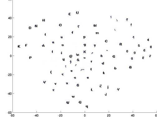
(a) Learnt embedding of characters using tsne.

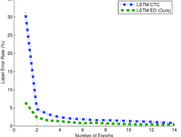
(b) Convergence of lstm-ctc and lstm-ed.

Figure 3: Plot showing character embedding and convergence of lstm-ctc and lstm-ed.

5 Conclusion

We demonstrate the applicability of sequence to sequence learning for word prediction in printed text ocr. Fixed length representation for variable length input using a recurrent encoder-decoder architecture sets us apart from present day state of the art algorithms. We believe with enough memory space availability, sequence to sequence regime could be a better and efficient alternative for ctc based networks. The network could well be extended for other deep recurrent architectures with variable length inputs, e.g. attention based model to describe the image contents etc.

References

- (1) ABBYY OCR ver. 9. http://www.abbyy.com/.
- (2) Tesseract Open-Source OCR. http://code.google.com/p/tesseract-ocr/.
- Cho et al. (2014) Cho, Kyunghyun, van Merrienboer, Bart, Gülçehre, Çaglar, Bougares, Fethi, Schwenk, Holger, and Bengio, Yoshua. Learning phrase representations using RNN encoder-decoder for statistical machine translation. CoRR, 2014.
- Chung et al. (2014) Chung, Junyoung, Gülçehre, Çaglar, Cho, KyungHyun, and Bengio, Yoshua. Empirical evaluation of gated recurrent neural networks on sequence modeling. CoRR, 2014.
- Graves et al. (2006) Graves, Alex, Fernández, Santiago, Gomez, Faustino, and Schmidhuber, Jürgen. Connectionist temporal classification: Labelling unsegmented sequence data with recurrent neural networks. In ICML, 2006.
- Hinton et al. (2012) Hinton, Geoffrey E., Deng, Li, Yu, Dong, Dahl, George E., Mohamed, Abdel-rahman, Jaitly, Navdeep, Senior, Andrew, Vanhoucke, Vincent, Nguyen, Patrick, Sainath, Tara N., and Kingsbury, Brian. Deep neural networks for acoustic modeling in speech recognition:the shared views of four research groups. Signal Processing Magazine, 2012.
- Hochreiter & Schmidhuber (1997) Hochreiter, Sepp and Schmidhuber, Jürgen. Long short-term memory. Neural Comput., 1997.
- Krizhevsky et al. (2012) Krizhevsky, Alex, Sutskever, Ilya, and Hinton, Geoffrey E. Imagenet classification with deep convolutional neural networks. In NIPS, 2012.
- Kumar et al. (2007) Kumar, Anand, Jawahar, C. V., and Manmatha, R. Efficient search in document image collections. In ACCV, 2007.
- Lowe (2004) Lowe, David G. Distinctive image features from scale-invariant keypoints. IJCV, 2004.
- Sutskever et al. (2011) Sutskever, Ilya, Martens, James, and Hinton, Geoffrey. Generating text with recurrent neural networks. In ICML, 2011.
- Sutskever et al. (2014) Sutskever, Ilya, Vinyals, Oriol, and Le, Quoc V. Sequence to sequence learning with neural networks. CoRR, 2014.
- Tieleman & Hinton (2012) Tieleman, T. and Hinton, G. Lecture 6.5 - rmsprop, coursera: Neural networks for machine learning. Technical report, 2012.
- van der Maaten & Hinton (2008) van der Maaten, L.J.P and Hinton, G.E. Visualizing high-dimensional data using t-sne. JMLR, 2008.
- Vinyals & Le (2015) Vinyals, Oriol and Le, Quoc V. A neural conversational model. CoRR, 2015.
- Vinyals et al. (2014) Vinyals, Oriol, Toshev, Alexander, Bengio, Samy, and Erhan, Dumitru. Show and tell: A neural image caption generator. CoRR, 2014.
- Zaremba & Sutskever (2014) Zaremba, Wojciech and Sutskever, Ilya. Learning to execute. CoRR, 2014.