The NuSTAR Extragalactic Surveys: Initial results and catalog from the Extended Chandra Deep Field South

Abstract

We present initial results and the source catalog from the NuSTAR survey of the Extended Chandra Deep Field South (hereafter, ECDFS) – currently the deepest contiguous component of the NuSTAR extragalactic survey program. The survey covers the full $\approx$30′$\times$30′ area of this field to a maximum depth of $\approx$360 ks ($\approx 220$ ks when corrected for vignetting at 3-24 keV), reaching sensitivity limits of $\approx 1.3\times 10^{-14}~{}{\rm ergs~{}s^{-1}~{}cm^{-2}}$ (3-8 keV), $\approx 3.4\times 10^{-14}~{}{\rm ergs~{}s^{-1}~{}cm^{-2}}$ (8-24 keV) and $\approx 3.0\times 10^{-14}~{}{\rm ergs~{}s^{-1}~{}cm^{-2}}$ (3-24 keV). Fifty four (54) sources are detected over the full field, although five of these are found to lie below our significance threshold once contaminating flux from neighboring (i.e., blended) sources is taken into account. Of the remaining 49 that are significant, 19 are detected in the 8-24 keV band. The 8-24 keV to 3-8 keV band ratios of the twelve sources that are detected in both bands span the range 0.39–1.7, corresponding to a photon index range of $\Gamma\approx 0.5-2.3$, with a median photon index of $\overline{\Gamma}=1.70\pm 0.52$. The redshifts of the 49 sources in our main sample span the range $z=0.21-2.7$, and their rest-frame 10-40 keV luminosities (derived from the observed 8-24 keV fluxes) span the range $L_{\rm 10-40keV}\approx(0.7-300)\times 10^{43}~{}{\rm ergs~{}s^{-1}}$, sampling below the “knee” of the X-ray luminosity function out to $z\sim 0.8-1$. Finally, we identify one NuSTAR source that has neither a Chandra nor an XMM-Newton counterpart, but that shows evidence of nuclear activity at infrared wavelengths, and thus may represent a genuine, new X-ray source detected by NuSTAR in the ECDFS.

1. Introduction

Extragalactic X-ray surveys have revolutionized our understanding of the accretion of matter on to supermassive black holes. Collectively they have provided a census of active galactic nuclei (AGN) across broad swathes of parameter space, enabling astronomers to relate black hole growth to fundamental properties such as large-scale environment and host galaxy characteristics (e.g., stellar mass, age, morphology; see the reviews of Alexander & Hickox 2012 and Brandt & Alexander 2015). Indeed, the deepest Chandra and XMM-Newton surveys identify significant populations (i.e., $\sim$tens) of AGNs beyond $z\sim 3$ (e.g., Alexander et al. 2003; Luo et al. 2008; Hasinger 2008; Elvis et al. 2009; Civano et al. 2012; Brusa et al. 2009; Laird et al. 2009; Xue et al. 2011; Goulding et al. 2012; Ranalli et al. 2013), probing the history of black hole growth over $\gtrsim 80\%$ of the age of the Universe. Such surveys have resolved almost all ($\approx$70–90%) of the Cosmic X-ray Background (hereafter, CXB; Giacconi et al. 1962) at 0.5-8 keV (e.g., Worsley et al. 2005; Hickox & Markevitch 2006; Lehmer et al. 2012; Xue et al. 2012).

Despite their undeniable success in identifying and characterizing the AGN population to high redshifts, Chandra and XMM-Newton are only sensitive to observed-frame photon energies $\lesssim$10 keV. This represents a significant limitation as it is known from earlier, non-focussing, X-ray missions that the CXB peaks at $\approx$20–40 keV (e.g., Marshall et al. 1980; Gruber et al. 1999; Frontera et al. 2007; Churazov et al. 2007; Ajello et al. 2008). Until recently, the most advanced X-ray telescopes sensitive to these energies have resolved only 1–2% of this peak into individual sources (e.g., Krivonos et al. 2007; Ajello et al. 2008; Bottacini et al. 2012). As such, the sources that make up the peak of the CXB are almost wholly unconstrained by direct observations, with the best constraints instead coming from population synthesis models (i.e., using spectral models to extrapolate the X-ray spectra of the source populations detected at lower energies; e.g., Setti & Woltjer 1989; Madau et al. 1994; Comastri et al. 1995; Gilli et al. 2001; Treister & Urry 2005; Gilli et al. 2007; Treister et al. 2009; Ballantyne et al. 2011). Many such models require a significant population of Compton-thick AGNs (i.e., obscured by absorbing column densities, $N_{\rm H}>1.5\times 10^{24}~{}{\rm cm^{-2}}$, the inverse of the Thomson cross section) to reproduce the peak of the CXB. However, these predictions are heavily influenced by the spectral assumptions used to extrapolate the X-ray spectra to $>10$ keV, and strong degeneracies exist between the assumed model parameters (e.g., Ballantyne et al. 2006; Gilli et al. 2007; Treister et al. 2009; Akylas et al. 2012).

Recent progress in characterizing the hard X-ray output from the AGN population has been made by studies exploiting data collected by the INTEGRAL and Swift telescopes (e.g. Krivonos et al. 2007; Tueller et al. 2008; Ajello et al. 2008; Burlon et al. 2011; Ajello et al. 2012; Vasudevan et al. 2013). These studies report that $\sim 5-25\%$ of local AGNs are confirmed on the basis of X-ray spectral analyses to be Compton-thick (to $N_{\rm H}\sim 10^{25}~{}{\rm cm^{-2}}$). However, the limited sensitivity of these telescopes means that they can only probe the most local ($\lesssim 100$ Mpc) AGNs to the depth needed to verify Compton-thick levels of absorption, leaving no constraints on the evolution of the absorbed fractions of AGNs. The Nuclear Spectroscopic Telescope Array (hereafter, NuSTAR; Harrison et al. 2013) is a factor of $\sim 10^{2}$ more sensitive than previous high energy X-ray telescopes and is predicted to determine the make up of 25-35% of the CXB (Ballantyne et al. 2011), allowing us to measure the contribution from heavily obscured AGNs over truly cosmological scales. To achieve this science goal NuSTAR has undertaken four extragalactic surveys, spanning a range of different combinations of area and depth, with the deepest observations identifying more common, faint sources. The complementary shallower, wider surveys that will cover rarer, more extreme sources. The tiers that make up the NuSTAR extragalactic survey are (a) a large area (currently covering $\approx$7 deg².), mostly shallow serendipitous survey consisting of the areas around targeted sources (described in Alexander et al. 2013 and Lansbury et al. in prep.), (b) a mid-depth ($\approx 90~{}ks$ maximum unvignetted depth) survey of the 2 deg². Cosmic Evolution Survey (COSMOS; Scoville et al. 2007), described in Civano et al. (submitted) and (c) two deep ($\approx 360$ ks maximum unvignetted depth), small area surveys of the $\approx$0.25 deg². Extended Chandra Deep Field South (hereafter, ECDFS; Lehmer et al. 2005, hereafter L05) – the focus of this study – and the $\approx$0.24 deg². Extended Groth Strip (i.e., EGS; NuSTAR analysis to be presented in Aird et al. in prep.). By concentrating on extragalactic fields, these surveys will give a census of hard X-ray sources that is unbiased by pre-selection, enabling the characterization of a significant sample of the “typical” population responsible for the bulk of the CXB. Indeed, NuSTAR has already demonstrated this capability in the case of the ECDFS source NuSTAR J033202-2746.8. Prior to NuSTAR the spectral properties of this source were incorrectly constrained, but it has since been shown to be a high-redshift QSO with a significant reflection component, despite being Compton-thin (Del Moro et al. 2014). If such reflection is common within the obscured – but sub-Compton-thick – AGN population, it would have a significant impact on our understanding of the make up of the CXB.

In this study, we describe the NuSTAR observations of the ECDFS that form one of the two deepest contiguous components of the NuSTAR extragalactic survey (see §2.1). In §2.2 we describe the data reduction and processing steps we took to form the final science, background and exposure mosaics. In §2.3, we describe how we obtained our “blind” source catalog, the format of which is described in our Appendix. In §3 we describe the first results from this sample of sources including derived properties such as source fluxes, spectral indices and luminosities. We discuss constrains on the number of sources not detected by either Chandra nor XMM-Newton in §4. In §5 we give a brief overview of the NuSTAR detected sources in the context of the previously known X-ray sources in this field. Finally, in §6, we summarize our results. We adopt $H_{0}=71$ km s^-1 Mpc^-1, $\Omega_{\rm M}=0.27$, and $\Omega_{\Lambda}=0.73$ and use the AB-magnitude system throughout (where appropriate).

2. Observations and analyses

The NuSTAR ECDFS survey consists of observations from two separate passes. Observations making up the first pass were taken between September and December 2012, while those making up the second pass were taken roughly six months later between March and April 2013. The details of these observations, including aim points, roll angles and useable exposure times are provided in Table 1. In this section we describe our observing strategy and outline the steps taken to process and analyze the resulting data. We note that, in order to ensure consistency between the different components of the NuSTAR extragalactic surveys, a determined effort was made to follow the same analysis techniques for both COSMOS (Civano et al. submitted) and the ECDFS surveys wherever possible.

2.1. Observing strategy

Table 1Details of the individual observations that make up the two NuSTAR passes of the ECDFS

(1)	(2)	(3)	(4)	(5)	(6)
Exp. ID	Obs. Date	R.A.	Dec	Roll Angle	$t_{\rm Exp}$
1	28 Sep. 2012	52.93	$-27.97$	85.28	44.9
2	29 Sep. 2012	53.06	$-27.97$	85.30	45.6
3	30 Sep. 2012	53.18	$-27.97$	85.30	47.1
4	01 Oct. 2012	53.31	$-27.97$	85.31	47.0
5	02 Oct. 2012	52.93	$-27.86$	85.30	46.3
6	04 Oct. 2012	53.06	$-27.86$	85.31	45.4
7	30 Nov. 2012	53.18	$-27.86$	264.99	47.9
8	01 Dec. 2012	53.31	$-27.86$	264.96	48.0
9	03 Dec. 2012	52.93	$-27.75$	266.96	46.7
10	04 Dec. 2012	53.06	$-27.75$	266.94	47.7
11	05 Dec. 2012	53.18	$-27.75$	266.93	48.0
12	06 Dec. 2012	53.31	$-27.75$	266.88	48.4
13	07 Dec. 2012	52.93	$-27.64$	266.92	48.8
14	08 Dec. 2012	53.06	$-27.64$	266.94	49.2
15	09 Dec. 2012	53.18	$-27.64$	266.94	49.4
16	10 Dec. 2012	53.30	$-27.64$	266.95	46.5
17	15 Mar. 2013	53.30	$-27.64$	351.82	48.6
18	17 Mar. 2013	53.18	$-27.64$	351.81	48.9
19	18 Mar. 2013	53.06	$-27.64$	351.83	48.6
20	19 Mar. 2013	52.93	$-27.64$	351.84	46.1
21	20 Mar. 2013	53.31	$-27.75$	351.83	46.4
22	21 Mar. 2013	53.18	$-27.75$	351.84	46.1
23a	22 Mar. 2013	53.06	$-27.75$	351.86	31.0
23b	23 Mar. 2013	53.06	$-27.75$	351.88	15.2
24	24 Mar. 2013	52.93	$-27.75$	356.88	45.7
25	25 Mar. 2013	53.31	$-27.86$	356.88	46.0
26	26 Mar. 2013	53.18	$-27.86$	356.89	45.9
27	27 Mar. 2013	53.06	$-27.86$	1.97	45.4
28	28 Mar. 2013	52.93	$-27.86$	1.95	45.4
29	29 Mar. 2013	53.31	$-27.97$	1.94	45.3
30	30 Mar. 2013	53.18	$-27.97$	1.93	45.2
31	31 Mar. 2013	53.06	$-27.97$	1.93	45.2
32	01 Apr. 2013	52.93	$-27.97$	1.95	45.0

NuSTAR features two independent telescopes with corresponding focal plane modules (hereafter, referred to as FPMA and FPMB), that simultaneously observe the same patch of sky during each observation. Each focal plane has a $\approx$12′$\times$12′ field of view and consists of four CdZnTe detectors. The physical pixels are 12″ on a side, with the scale subdivided into 2.46″ pixels in the software. While the detectors are sensitive to photon energies in the range 3-100 keV, the optics of the telescope limit this range to 3-78.4 keV. The focusing optics of NuSTAR give it an unprecedented angular resolution at these hard X-ray energies, with a tight central “core” of FWHM=18″ and a half-power diameter of 58″, meaning surveys as deep as the ECDFS are not limited by confusion between detected sources. The area covered by the ECDFS (i.e., $\approx$30′$\times$30′; L05) is larger than the NuSTAR field of view, so we adopted a tiling strategy to provide full coverage of the field. A strategy of 16 pointings separated by a half-detector shift – forming a 4$\times$4 square – was chosen based on the findings of pre-survey tests which suggested that this optimizes the number of detections in the field. Since the roll angle of the observatory is a function of time, the observing schedule was chosen not only to ensure that the edges of each observation were roughly aligned, but also to align them with the Chandra coverage of this field.

Each pointing had an effective exposure of approximately 45 ks per pass, and all but one of the pointings consisted of a single unbroken exposure, resulting in a total of 33 exposures. Table 1 gives the precise useable integration times for each of the 33 separate exposures after filtering out flaring events (see §2.2.1). The total time spent on the ECDFS across both passes was 1.49 Ms. On completion of the two passes, the central, deepest $\approx 20$′$\times 20$′ region of the field was covered by eight separate pointings, and thus observed for a total of $\sim 360$ ks, while the edges had been covered by four pointings (i.e., to $\sim 180$ ks) and the corners by two (i.e., to $\sim 90$ ks). The cumulative area histogram showing the area of the sky covered to a given exposure time is shown in 1.

2.2. Production of science, background and exposure maps

In this subsection, we outline the detailed steps we took to produce the final mosaics, identify sources and derive source properties. All data reduction was performed using v6.15 of HEASoft, v1.3 of the NuSTAR developed software, NuSTARDAS (included with v6.15 of HEASoft), and v4.5 of CIAO.

Figure 1.— Cumulative area above a given exposure time in the 3-24 keV band for the final mosaic in a single focal plane module. The dotted line gives the total area above a given exposure before correcting for vignetting, whereas the solid line includes the effects of vignetting on the total exposure.

2.2.1 Reprojection, bad pixels rejection, energy bands.

Each of the 33 exposures results in two event files, one each for FPMA and FPMB. These 66 raw, unfiltered event files were processed and reprojected using the NuSTARDAS program nupipeline to produce 66 clean event files. Inspection of the cleaned event files revealed that four exposures (Exp. IDs 2, 3, 18 and 22 in Table 1) had been significantly affected by flaring events. These events were filtered out using CIAO’s dmgti tool to make a user-defined good time interval (gti) file, binning in 20 s intervals and rejecting periods when the average binned count rate exceeded $0.6~{}{\rm cts\ s^{-1}}$ (within the whole observable energy range, i.e., 3-78.4 keV), a threshold selected through visual inspection of the light curves. This filtering removed a total of 6.0 ks of exposure time, representing $\approx 0.4\%$ of the total exposure time for the two passes. Following Alexander et al. (2013) the final cleaned event files were split into three energy bands, 3-8 keV, 8-24 keV, and 3-24 keV, using HEASoft’s extractor tool. The 24 keV upper band energy is chosen to optimize signal to noise for sources with average spectral properties. For these sources, the combination of photon spectrum falling rapidly with energy, flat background and decreasing effective area means that detection significance decreases with increasing high energy cut-off. As a check, we generated a fourth, 24-40 keV band, but no significant sources were identified using the detection technique described below.

2.2.2 Background map generation

The majority of counts in all of the ECDFS observations are attributable to background that arises from: (1) an instrumental background component that dominates at energies $\gtrsim 20$ keV; (2) a focussed background component that is made up of X-ray emitting sources that are focussed by the telescope optics but lie below the detection threshold; (3) an “aperture” background that is astronomical in origin, but is due to X-ray photons that have not scattered off (and thus have not been focussed by) the telescope optics; (4) a spatially uniform component that is strong at $\lesssim 5$ keV, probably due to neutrons striking the detector; and (5) another low energy component that is related to solar photons reflecting off the back of the aperture stop. The aperture background dominates the photon counts at $\lesssim 30~{}{\rm keV}$ and, as such, most strongly affects our chosen energy bands.

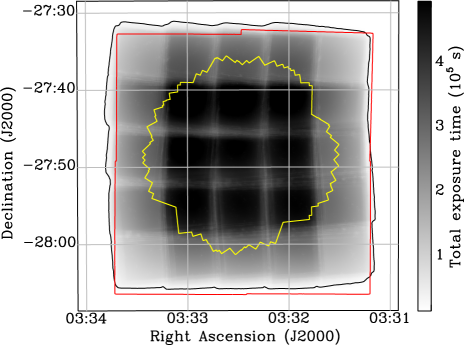
Figure 2.— Vignetting-corrected exposure map showing the effective exposure of the field, combining both FPMA and FPMB. Darker grays imply longer effective exposures (see colorbar). The black line shows the limit of the NuSTAR exposure, while the red and yellow lines show the limits of the 250 ks Chandra ECDFS (L05) and 4 Ms CDFS (Xue et al. 2011) exposures, respectively.

Due to the asymmetric layout of the optics bench, the aperture background has a strong gradient that differs between FPMA and FPMB, making it difficult to subtract by the usual process of extrapolating from regions around the source. This is especially true in the case of overlapping observations such as those that make up the ECDFS mosaic. Instead, we use a model of the aperture background for each FPM produced using the specially developed IDL software nuskybgd (Wik et al. 2014). The X-ray spectrum is extracted from a set of user-defined background regions and then fit with a pre-defined model consisting of the five components listed above (note that component $[4]$ is incorporated into the instrumental background, i.e., component $[1]$). A set of pre-determined maps that describe the spatial distribution of each background component in each energy band (see Wik et al. 2014) are then adjusted using the normalizations of the spectral fit.

When generating the model background, there is the option in nuskybgd to exclude known bright sources in each image from the user-defined regions to prevent them from being inappropriately included in the background estimation. We experimented with excluding known bright sources, but they were found to have no significant impact on either our final detected source list or source fluxes. In light of this, and for reproducibility, we chose not to exclude sources in generating our final background maps. Instead, we simply used four large (i.e., $\sim 5$′ on a side) square regions centered on the four chips that make up each detector to define our background regions (i.e., using the same procedure as for the NuSTAR-COSMOS survey described in Civano et al. (submitted).

A highly accurate synthetic background map is crucial to determine source reliability and calculate net source counts and, ultimately, fluxes. To test the reliability of the synthetic background maps we calculated the relative difference between the number of counts extracted from 3,500 30″ radius regions distributed across the “synthetic” background and the number of counts extracted in the same regions distributed across the science mosaics (i.e., $(C_{\rm Sci}-C_{\rm Bgd})/C_{\rm Sci}$). The resulting values are normally distributed with a dispersion ($\sigma$) of 0.078, 0.064 and 0.053 centered around $1.7\times 10^{-3}$, $-1.9\times 10^{-3}$ and $-4.4\times 10^{-3}$ for the 3-8 keV, 8-24 keV and 3-24 keV bands, respectively (FPMA and FPMB combined). Tests conducted on mock science images (i.e., Poissonian realizations of the background maps) demonstrated that this dispersion is consistent with that expected due to Poisson noise, meaning that the uncertainties introduced by the background estimation are small compared to those due to the noise in the data.

2.2.3 Exposure maps and vignetting

Exposure maps were generated using the NuSTARDAS software nuexpomap. As well as pointing information, this also takes into account the movement of NuSTAR’s 10 m long mast when determining the exposure time of each point on the sky translated into pixel position. To reduce processing time, there is the option to reduce the number of calculations by spatially binning the exposure maps. We therefore spatially bin our exposure maps over 5 pixels in each dimension, which is smaller than the 30″ aperture used for photometry measurements and thus has negligible influence on our flux measurements while speeding up processing by a factor of $\sim 5^{2}=25$.

The effects of vignetting were also taken into account with nuexpomap to generate effective exposure maps for each observation. The degree of vignetting is energy-dependent, but generating a vignetting map for every energy channel is prohibitive. Instead, following Civano et al. (submitted), we calculated the energy that minimizes the difference across the three adopted energy bands by convolving the instrument response with a power-law spectrum of $\Gamma=1.8$ (i.e., the average of nearby AGN studied at $>10$ keV; Burlon et al. 2011). This results in three energies which we used to generate the effective exposure maps: 5.42 keV for the 3-8 keV band, 13.02 keV for the 8-24 keV band, and 9.88 keV for the 3-24 keV band. We calculate that this approximates the vignetting in each energy channel to within 14.5% for all three bands, the difference being largest farthest from the aim point. The effects of applying this vignetting correction are shown in Figure 1, in which the solid line shows the cumulative solid angle to a given effective exposure, evaluated at 3-24 keV. On average, correcting for vignetting reduces the nominal exposure time by a factor of $\sim 2$.

2.2.4 Astrometric correction

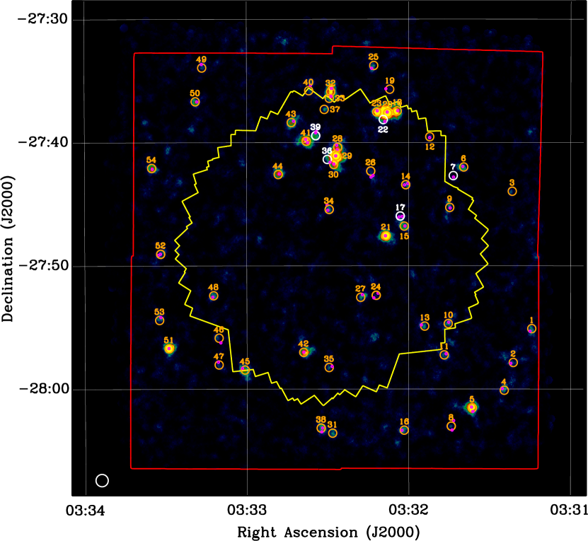
Figure 3.— False-probability ($P_{\rm False}$) map produced by combining data in the 3-24 keV band from both FPMA and FPMB. Blue, green and, finally, yellow shading indicates areas of increasingly lower $P_{\rm False}$, and thus the regions most likely to be associated with genuine sources. The yellow and red lines indicate the extent of the the 4 Ms CDFS (Xue et al. 2011) and 250 ks Chandra-ECDFS (L05) surveys, respectively. The white circle in the bottom-left of the figure indicates the size of the 30″-radius aperture used for measuring source photometry. The positions of all NuSTAR sources found using our detection algorithm (see §2.3.1) are indicated with small numbered circles (the numbers refer to the source ID in the online catalog). Orange circles indicate those that remain significant (i.e., meet our significance thresholds) after taking into account the effects of neighboring sources (i.e., after source deblending; see §2.3.2), whereas the white circles indicate those that no longer prove to be significant. Note that in some instances the position does not correspond to that of the minimum $P_{\rm False}$ in the 3-24 keV band. This is because those sources are detected at a higher significance in another band and, as such, the position is based on the minimum $P_{\rm False}$ position in that other band (see §2.3.1). Small magenta circles indicate the positions of the Chandra or XMM-Newton counterparts to the NuSTAR-detected sources.

Before combining the individual observations to form the final science, exposure and background mosaics, we experimented with correcting for astrometric offsets between individual exposures. In brief, we stacked the NuSTAR data at the positions of known Chandra-detected sources and used the relative positions of the stacked detected source to perform first order (i.e., x-y shift) astrometric corrections. However, we found that this correction had no measurable impact on either the list of detected sources, nor their measured fluxes. As such, we chose to not include any astrometric correction in the rest of our analyses in order to keep the analysis stream as simple as possible. Based on their analysis of simulated NuSTAR observations of the COSMOS field, Civano et al. (submitted) estimate an average positional uncertainty of 6.6″, which, due to the many similarities between the ECDFS and COSMOS NuSTAR survey strategies and data reduction, we adopt as the positional uncertainty for the detected ECDFS sources.

2.2.5 Mosaicing

To create a set of contiguous maps, the individual science, background and exposure images were mosaiced using HEASoft’s ximage package. Our experimentation with astrometry correction (see §2.2.4) demonstrated that the frames from both FPMA and FPMB are co-aligned to within measurable tolerances, so we are able to combine the data from these two modules by adding together the equivalent mosaics, thereby increasing the sensitivity of the final combined mosaic. The final mosaiced vignetting-corrected exposure map, combining FPMA and FPMB, is shown in Figure 2. All source detection and derived photometric measurements are taken from the combination of the FPMA and FPMB mosaics.

Figure 4.— Same as Figure 3, but for the 8-24 keV band. Sources shown are only those that are detected in this band.

2.3. Source detection and calculation of derived properties

In this subsection we detail how we produced our source catalog from the final science, background and exposure maps. We adopted a multi-stage approach which successfully separates nearby sources and ensures that all significant sources are identified, while maintaining a low number of false-positive detections. The steps are:

1. we first generate a seed list of potential sources in each band using our source detection procedure and a low significance detection threshold;

2. we combine the seed lists from each band using positional matching and those not meeting our final, more stringent false-probability cut in any band are excised from the list to form our final catalog;

3. we perform aperture photometry at the positions of the sources in our final catalog;

4. we perform deblending (see §2.3.2) on the sources in the final catalog to account for the flux contribution from neighboring significant sources; those sources that prove to be below our significance threshold post-deblending are flagged, but are retained in the final catalog.

A full description of each of these steps is provided below.

2.3.1 Initial source seed list

The strong, spatially varying background of the NuSTAR ECDFS mosaics (see §2.2.2) makes blind source detection challenging. Considerable testing with CIAO’s wavdetect source-identification algorithm (Freeman et al. 2002) revealed that it is not designed to deal with the deep NuSTAR data in the ECDFS, and it identified large numbers (i.e., $\sim$200) of false-positive detections, particularly in the outer regions of the field, likely due to the high background of NuSTAR images compared to the Chandra data for which wavdetect was originally developed to analyze. As a consequence, we instead employed the alternative approach of performing source detection directly on false-probability (hereafter, $P_{\rm False}$) maps generated from the mosaics. These $P_{\rm False}$ maps, which we calculate using the incomplete Gamma function (see Georgakakis et al. 2008), give the likelihood that the signal at each position in the mosaic is due to random fluctuations in the supplied background (i.e., not due to a real source). The maps were produced by passing smoothed science and background images to IDL’s igamma function, which computes the incomplete Gamma function at every position in the mosaics, i.e.,

$$P_{\rm False}={\tt igamma}({\rm Sci,Bgd})$$ (1)

where Sci and Bgd are the smoothed science and background mosaics, respectively. Two different smoothing lengths comprised of 10″ and 20″-radius top-hat functions were employed; the smaller radius helps separate adjacent sources, while the larger helps to identify fainter sources. Smoothed $P_{\rm False}$ maps were generated for each of our three energy bands and source detection was performed separately on each. Figure 3 shows the 20″-smoothed $P_{\rm False}$ map for the 3-24 keV band mosaic.

We used the SExtractor source detection algorithm (Bertin & Arnouts 1996) to identify regions of the $P_{\rm False}$ maps below a given threshold. Since SExtractor is designed to identify peaks in an image, we provided the log of the inverse $P_{\rm False}$ maps as input. The SExtractor detection algorithm requires a number of input parameters, the most important of which for our purposes is the threshold above which (in the inverse map) a source is considered to be significant. Poisson realizations of the blank background maps (see §2.2.2) were used to set the thresholds in each band. These Poisson realizations were treated as input science images and analyzed using the same procedures as the real science maps. By running our source detection algorithm on 100 realizations of these simulated, blank maps, we determined the $P_{\rm False}$ value below which we should expect, on average, one false-positive detection per ECDFS area per band and set those as our thresholds. This corresponds to thresholds of ${\rm log}(P_{\rm False})\leq-5.19,\leq-5.22$ and $\leq-5.34$ in the 3-8 keV, 8-24 keV and 3-24 keV bands, respectively. We note that these thresholds correspond to $\approx 99\%$ reliability, as evaluated by the simulated NuSTAR observations described in Civano et al. (submitted). Based on our Poisson realizations, there is a 34%, 42%, 19%, 3%, 1% and 1% likelihood that the 3-24 keV band mosaic contains 0, 1, 2, 3, 4 and 5 false positive detections (i.e., have ${\rm log}(P_{\rm False})\leq-5.34$). For the generation of our seed catalog we employ a somewhat more liberal threshold of ${\rm log}(P_{\rm False})\leq-4.5$ in all three bands to ensure that we detect all potential sources and employ the more stringent thresholds in our final cut after combining sources detected in each band (see §2.3.2). As the input maps have already been smoothed, we consider even a single pixel above these thresholds to be a potential source. The coordinates of each detection are taken as the position of the local minimum $P_{\rm False}$ (rather than, for example, the centroid) to maximize the likelihood that it will satisfy our more stringent final threshold cuts.

As we are performing separate source detection on images smoothed by two different smoothing lengths, SExtractor often identifies multiple nearby detections associated with the same source. If these were left in our seed catalog, they would lead to over-deblending at the deblending stage (i.e., the source flux would be erroneously deblended into these multiple detections). To account for this, for each seed detection we identify all other seed detections within a 30″ radius (the radius of the aperture used for photometry measurements) and retain the detection with the lowest $P_{\rm False}$ in our 20″-smoothed maps (even if initially detected in the 10″-smoothed maps). Again, this is done to increase the likelihood that a detection in our seed catalog will ultimately satisfy our final significance cut.

We take a similar approach to match sources identified in our three different energy bands. For each detection in the 3-24 keV band we identify the nearest source within a 30″ search radius in the other two energy bands, resulting in up to three different positions (i.e., one position for each band). Our final position is taken from the band giving the lowest $P_{\rm False}$ (based on a 20″ radius smoothing) to again maximize the likelihood that it will pass our final significance cut. All further analyses (i.e., aperture photometry, deblending) are performed using this final position.

After combining the seed catalogs from the three separate bands, we apply our more conservative $P_{\rm False}$ cuts. For this, we calculate the seed source $P_{\rm False}$ in each band based on a 20″ extraction radius (irrespective of whether the source was detected at 10″ or 20″-radius smoothing), and remove those that do not meet our final cuts (i.e., ${\rm log}(P_{\rm False})\leq-5.19,\leq-5.22$ and $\leq-5.34$ in the 3-8 keV, 8-24 keV and 3-24 keV bands, respectively). We also remove any sources in areas of low exposure (i.e., $<4\times 10^{4}$ s, corresponding to $\lesssim 10\%$ of the peak vignetted survey exposure).

In total, the above procedure returned 54 sources detected in at least one band that constitute our final source catalog. Aperture photometry was performed at the positions of these significant, detected sources followed by deblending, as described in the following subsection.

2.3.2 Net counts and deblending

We derive net counts, count rates and fluxes at the positions of all the significantly detected sources identified using the procedure described above. To determine total (i.e., source $+$ background) counts for our detections, we summed the total number of counts within 30″ of the final source position in the combined (i.e., FPMA$+$FPMB) science mosaics. This aperture size was chosen as a compromise between attempting to maintain as low an aperture correction as possible (a factor of 2.24 for 30″), and reducing the level of contamination from neighboring sources. Furthermore, tests showed that, compared to using 15″ and 45″ apertures, 30″ led to NuSTAR 3-8 keV fluxes that most closely matched those derived from Chandra observations (see §§2.3.3 and 2.3.4). Total background-only counts were calculated in the same size apertures centered on the positions of our detected seeds using the background images described in §2.2.2. The net number of counts for each detection was calculated by subtracting the background counts from the total counts. The upper and lower 1$\sigma$ confidence limits on the total source counts are calculated following Gehrels (1986). To this we add the background error ($\sigma_{\rm Bgd}$) in quadrature with the source count error to derive the error on the net count rate, scaling the background counts by a factor of 125, which is roughly the ratio between the area of the 30″ aperture used for photometry measurements and the total area over which the background model is defined (i.e., $=4\times 5\arcmin\times 5\arcmin$), i.e.,

$$\sigma_{\rm Bgd}=(1+\sqrt{125C_{\rm Bgd}+0.75})/125$$ (2)

where $C_{\rm Bgd}$ is the total number of background counts extracted from the background image described in §2.2.2.

The relatively extended PSF of NuSTAR means we must factor-in the contribution from neighboring detections to the measured count rates and fluxes. To deblend a given detection in our final catalog we assume that the net photon counts within the adopted 30″ radius aperture is the sum of that due to that detected source, plus the contribution from any other NuSTAR-detected sources within 90″(all the sources in the ECDFS are faint enough for any contribution from sources outside this radius to be considered negligible). While we acknowledge that there will also be some contribution from NuSTAR-undetected sources, our goal here is to produce a catalog based solely on NuSTAR data, rather than relying on prior (e.g., Chandra or XMM-Newton) information. We make the simplifying assumption that the contribution of a neighboring source is a function of only its brightness and separation from the source of interest. Under this assumption, the problem of deblending reduces to a set of solvable linear simultaneous equations; e.g., in the case of three sources:

$$C_{T}^{1}=N(r_{1,1})C_{D}^{1}+N(r_{1,2})C_{D}^{2}+N(r_{1,3})C_{D}^{3}$$

$$C_{T}^{2}=N(r_{2,1})C_{D}^{1}+N(r_{2,2})C_{D}^{2}+N(r_{2,3})C_{D}^{3}$$ (3)

$$C_{T}^{3}=N(r_{3,1})C_{D}^{1}+N(r_{3,2})C_{D}^{2}+N(r_{3,3})C_{D}^{3}$$

where $C_{T}^{n}$ is the total net photon counts within the 30″ aperture of source $n$, $C_{D}^{n}$ is the deblended net photon count of source $n$ (again, within 30″) and $N(r_{n,m})$ is the relative normalization that takes into account the separation between the sources $n$ and $m$ (normalized to 1 at $N(r_{n,n}=0)$). In reality, this is complicated by the non-azimuthally symmetric PSF which lengthens with increasing off-axis angle. From simulations, we estimate that the effect of this to the deblended flux of our detected sources is small compared to photometric uncertainties, i.e., typically $\sim 8\%$. Positional uncertainties are not taken into account in calculating the uncertainties on deblended count rates, but uncertainties in $C_{T}$ are factored-in using a Monte-Carlo technique, whereby Gaussian noise (appropriate for the high net counts of our significantly detected sources) is added to each $C_{T}$ according to the uncertainty on this value. This is performed $10^{4}$ times for each source and the resulting distribution (which is closely approximated with a Gaussian due to regression to the mean) for $C_{D}$ is assumed to give the uncertainty on this value.

Table 2Polynomial coefficients for calculating fluxes and $\Gamma$

(1)	(2)	(3)	(4)	(5)	(6)
Property	$a_{0}$	$a_{1}$	$a_{2}$	$a_{3}$	$a_{4}$
$f_{\rm SB}$	6.38	0.78	-0.32	0.10	-0.01
$f_{\rm HB}$	21.01	-3.12	-0.27	0.19	-0.02
$f_{\rm FB}$	17.13	-4.38	-0.21	0.42	-0.06
$\Gamma$	1.27	-2.81	0.04	-0.06	-0.12

At this stage we also perform deblending assuming a 20″-radius aperture (compared to the 30″ used above for aperture photometry); recall that initial source detection is performed using both 10″ and 20″-radius smoothing (see §2.3.1). We then use these 20″ deblended counts, in conjunction with the background photon counts, to re-calculate the $P_{\rm False}$ of each source post-deblending and flag (but not remove) those that are no longer significant after deblending. Of the 54 sources in the final catalog, five are flagged as being no longer significant post-deblending, leaving 49 sources that are significant post-deblending.

From the deblended 30″-aperture net photon counts we calculate net count rates (and associated uncertainties) using the mean combined (i.e., the sum of both detectors) effective exposure time within a 30″ aperture of the detected seed position. Deblended 8-24 keV to 3-8 keV band ratios are calculated using the Bayesian Estimation of Hardness Ratios (BEHR) method described in Park et al. (2006). We report the median and upper and lower 68th percentiles (i.e., $1\sigma$ uncertainties) returned by this method. Photon indices and fluxes were calculated from these deblended band ratios and net count rates following the procedure described in the next subsection.

2.3.3 Flux calculation

Following the same basic approach as Alexander et al. (2013), observed deblended fluxes in each band and effective photon indices (i.e., $\Gamma$) were calculated from the deblended 30″ aperture count rates using conversion factors derived from XSPEC model spectra. To generate the conversion factors, we use XSPEC’s fakeit command to model power-law spectra spanning a range of power-law indices ($0.0<\Gamma<3.0$, in increments of 0.01; XSPEC model: pow) and taking the rmf and arf at the aim-point of the two detectors into account. “Fake” fluxes and count rates in the three bands were extracted from these synthetic spectra and were used to generate polynomial solutions that relate observed fluxes and photon indices to our observed count rates and 8-24 keV to 3-8 keV band ratios:

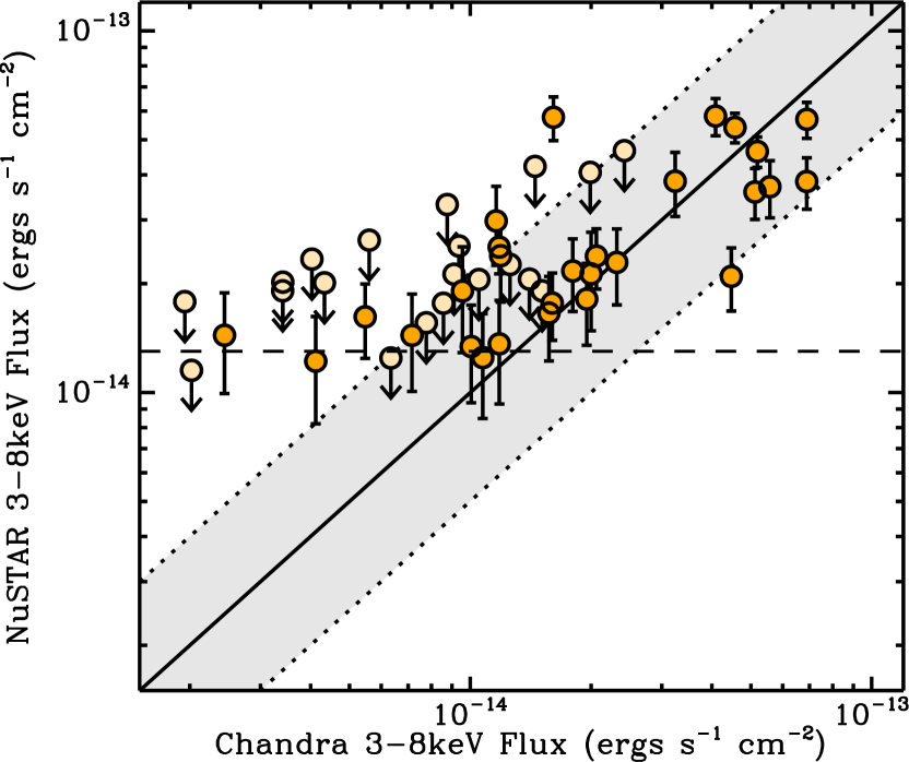
Figure 5.— Comparison of deblended, aperture-corrected NuSTAR 3-8 keV fluxes versus the Chandra-measured fluxes of all the Chandra sources within 30″ of the NuSTAR source position. Filled circles represent 3$\sigma$ detections, whereas open circles represent 3$\sigma$ upper limits. The solid line shows the 1:1 relation, while the grey shading indicates the region within a factor of 3 of this line. The dashed horizontal line indicates the sensitivity limit of the deepest region of the survey in the 3-8 keV band, i.e., $\approx 1.3\times 10^{-14}~{}{\rm ergs~{}s^{-1}~{}cm^{-2}}$.

$$\frac{f_{\rm E}}{R_{\rm E}}=10^{-14}\sum\limits_{i=0}^{n}a_{i}\Gamma^{i}$$ (4)

where

$$\Gamma=\sum\limits_{i=0}^{n}a_{i}b^{i}$$ (5)

and $f_{\rm E}$ is the flux within a given energy band (in ${\rm ergs\ s^{-1}\ cm^{-2}}$), $R_{\rm E}$ is the count rate in the same energy band (in ${\rm ks^{-1}}$), $b={\rm log}\left(R_{\rm 8-24\ keV}/R_{\rm 3-8\ keV}\right)$ (i.e., the logarithm of the 8-24 keV to 3-8 keV band ratio) and $\Gamma$ is the observed (i.e., not corrected for absorption) photon index. The polynomial coefficients for the above equations, $a_{i}$, are given in Table 2 and reproduce the XSPEC fluxes and photon indices to within $1\%$ across $-0.7<b<0.4$ (corresponding to $0.0<\Gamma<3.0$). Where a source is detected in both the 3-8 keV and 8-24 keV bands (and thus has a well constrained photon index), we use the derived photon index, otherwise we assume a fixed $\Gamma$ of 1.8 (corresponding to count rate to flux conversions of $7.2\times 10^{-14}$, $1.5\times 10^{-13}$ and $1.0\times 10^{-13}$ ${\rm ergs\ s^{-1}\ cm^{-2}\ ks}$ for the 3-8 keV, 8-24 keV and 3-24 keV bands, respectively). These flux conversions take the size of the aperture into account to return aperture-corrected fluxes (which are reported throughout).

To verify the accuracy of our process for calculating deblended NuSTAR fluxes, we carry out a comparison between the NuSTAR-derived 3-8 keV fluxes and the total Chandra-derived 3-8 keV fluxes arising from all Chandra sources within 30″ of the NuSTAR source position combined. This comparison is shown in 5. The NuSTAR fluxes cluster along the 1:1 line shown on this plot and all but two NuSTAR sources are consistent (within $3\sigma$ errors) with the total Chandra flux to within a factor of two, thereby validating our approach of calculating NuSTAR fluxes. We note that some of the scatter in this plot is expected to be introduced by intrinsic source variability (e.g., Paolillo et al. 2004; Young et al. 2012) and spurious matches between the NuSTAR and Chandra sources (see §2.3.4).

Figure 6.— Plot showing the solid angle of the survey below a given aperture-corrected flux sensitivity (shown on abscissa) corresponding to a S/N of 3 in each of our NuSTAR bands. These sensitivity limits were calculated from the background and exposure mosaics alone using the procedure outlined in §2.3.3. The most sensitive region in the 3-8 keV, 8-24 keV and 3-24 keV bands reach $\approx 1.3\times 10^{-14}$, $\approx 3.4\times 10^{-14}$ and $\approx 3.0\times 10^{-14}~{}{\rm ergs~{}s^{-1}~{}cm^{-2}}$. The dotted lines indicate the flux limits for an area of $\approx 630$ arcmin², which is roughly half the solid angle of the full NuSTAR ECDFS survey, and corresponds to values of $\approx 2.1\times 10^{-14}$, $\approx 5.1\times 10^{-14}$ and $\approx 4.4\times 10^{-14}~{}{\rm ergs~{}s^{-1}~{}cm^{-2}}$ for the 3-8 keV, 8-24 keV and 3-24 keV bands, respectively.

We can calculate the limiting flux at every point in the final mosaics using the background and exposure maps assuming the detection $P_{\rm False}$ thresholds introduced in §2.3.1 (i.e., ${\rm log}(P_{\rm False})\leq-5.19,\leq-5.22$ and $\leq-5.34$ in the 3-8 keV, 8-24 keV and 3-24 keV bands, respectively) and using the count rate to flux conversions above, assuming $\Gamma=1.8$. We use this to determine the area of the survey reaching a given flux limit in each of our bands, the results of which are shown in 6. The most sensitive regions of the survey reach $\approx 1.3\times 10^{-14}$, $\approx 3.4\times 10^{-14}$ and $\approx 3.0\times 10^{-14}~{}{\rm ergs~{}s^{-1}~{}cm^{-2}}$ in the 3-8 keV, 8-24 keV and 3-24 keV bands, respectively. We note, however, that these are the theoretical flux limits of the survey for isolated sources. In reality, the relatively large NuSTAR PSF may affect the total area to a given limit as regions around bright sources are less sensitive due to contamination and issues arising from deblending. A full understanding of these second-order factors will be necessary to obtain, e.g., source number counts and luminosity functions, to be published in Harrison et al. (in prep.) and Aird et al. (in prep.).

2.3.4 Multiwavelength counterparts, redshifts and luminosity determination

A major benefit of observing the ECDFS with NuSTAR is the wealth of ancillary multiwavelength data available for the field, making the characterization of identified sources comparatively straightforward. As much of these ancillary data have already been matched to sources identified in the Chandra and XMM-Newton observations of this field (i.e., the Chandra 250 ks ECDFS, Chandra 4 Ms CDFS and XMM-Newton 3 Ms ECDFS surveys; described in L05, Xue et al. 2011 and Ranalli et al. 2013, respectively), we obtain this information by matching to these previous X-ray catalogs. We first match to the Chandra-250 ks ECDFS catalog (L05) using a 30″ search radius. We report all matches that contribute at least 20% of the total flux from all Chandra sources within 30″ of the NuSTAR position (i.e., we ignore those faint Chandra sources that do not contribute significantly to the total Chandra flux within the search radius). Following this prescription, of the 54 sources in our final catalog, 48 were found to have at least one Chandra counterpart within the search radius. Of these, twelve NuSTAR sources were found to have two Chandra matches. No NuSTAR source was found to have more than two Chandra matches within the search radius. Of the 49 NuSTAR sources that are significant post-deblending, 44 have at least one Chandra counterpart.

Considering all 809 Chandra sources listed in L05 with our 30″ matching radius corresponds to a high spurious matching fraction of $\sim 70\%$ for our sample. However, we note that the majority (i.e., $\sim 85\%$ of matched Chandra counterparts have Chandra 3-8 keV fluxes $>2\times 10^{-15}~{}{\rm ergs~{}s^{-1}~{}cm^{-2}}$, of which there are 289 in the full L05 catalogue. Considering only these sources corresponds to a spurious matching fraction of $\sim 25\%$, which we consider to be a more reasonable estimation for the spurious matching fraction for our sample. Of course, following this logic, brighter Chandra counterparts are less likely to be spurious than fainter sources; we estimate the spurious matching fraction of $F_{\rm 3-8keV}>10^{-14}~{}{\rm ergs~{}s^{-1}~{}cm^{-2}}$ Chandra sources to be $\sim 3\%$, compared to $\sim 40\%$ for $F_{\rm 3-8keV}>10^{-15}~{}{\rm ergs~{}s^{-1}~{}cm^{-2}}$.

The six (of 54) sources without Chandra 250 ks counterparts were then matched against the Chandra-4 Ms CDFS catalog (again, using a 30″ search radius), which led to two further matches (and no multiple matches). Finally, the remaining four NuSTAR sources without counterparts were matched against the XMM-Newton 3 Ms catalog, which resulted in one further match. As a result, only three NuSTAR sources have no Chandra or XMM-Newton counterpart, all three of which are significant post-deblending.

Where a Chandra or XMM-Newton counterpart is identified, the associated optical counterpart is taken from the respective catalog (i.e., L05, Xue et al. 2011 or Ranalli et al. 2013 for Chandra-ECDFS, CDFS and XMM-Newton-ECDFS, respectively), together with its associated redshift, if available. We adopt the spectroscopic redshift in preference to the photometric redshift in cases where both are available. Of the 51 sources for which there are either Chandra or XMM-Newton counterparts, 46 have spectroscopic redshifts and three have only photometric redshifts (i.e., giving 49 in total). The corresponding numbers for those 49 sources that are significant post-deblending are: 41 with spectroscopic redshifts and three with photometric redshifts (i.e., 44 in total).

For those sources for which either spectroscopic or photometric redshifts are available, rest-frame $10-40$ keV (non-absorption corrected) luminosities were calculated from the 8-24 keV fluxes. $k$-corrections were performed by adopting the derived photon index for sources that significantly detected in both the 3-8 and 8-24 keV band, otherwise $\Gamma=1.8$ is assumed. In this work, we do not attempt to correct the luminosities for the effects of absorption; this will be the focus of a later study to combine Chandra and/or XMM-Newton data with the NuSTAR data to obtain the most reliable absorbing column densities (and hence, corrected luminosities) currently achievable (Del Moro et al. in prep; Zappacosta et al. in prep.).

3. Results

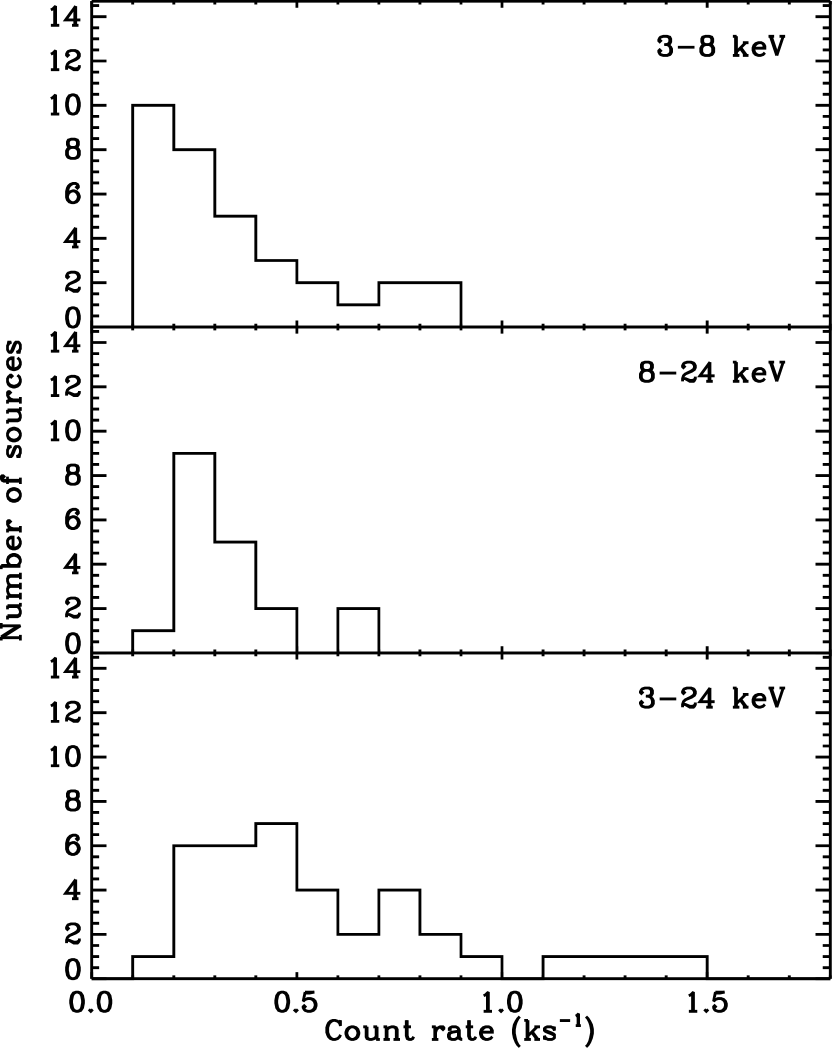
Figure 7.— Distributions of non-aperture corrected count rates in our three bands for the sources in the “blind” catalog. Here, we only include the 49 sources that pass our significance cuts post-deblending

In this section, we describe the properties of the detected sources and compare them against local (i.e., $z<0.3$) hard X-ray sources detected in the Swift-BAT survey and those in the NuSTAR serendipitous survey (Alexander et al. 2013). We also highlight three NuSTAR sources that are undetected in both the Chandra and XMM-Newton coverage of the ECDFS and CDFS, and which may therefore represent previously unknown contributors to the hard X-ray background.

3.1. Basic properties

As reported in §2.3.1, our final catalog contains 54 sources that are initially detected as significant in at least one of the three standard bands. However, of these 54, five are not significant after the effects of neighboring sources have been taken into account (i.e., after deblending). While these five are retained in the electronic catalog, the results described in the remainder of this paper consider only the 49 sources that are significant post-deblending.

It should also be noted that, since source detection is separate from photometry, some of our significantly detected sources (i.e., nine) have $<3\sigma$ counts in all three bands. As they pass our formal $P_{\rm False}$ threshold, these sources are retained in the electronic catalog and are considered in our general analyses and histograms, but are shown as $3\sigma$ upper limits in Cartesian plots.

Of the 49 sources that make up our final, post-deblended catalog, 12 are significant (i.e., satisfy the $P_{\rm False}$ cuts outlined in §2.3.1) in all three bands, 16 in exactly two (13 in 3-8 keV$+$3-24 keV, 3 in 8-24 keV$+$3-24 keV) and 8, 4, and 9 in the 3-8 keV, 8-24 keV and 3-24 keV bands only, respectively. As such, 19 are detected in the $8-24$ keV band, i.e., the photon energy range probed to unique depths by NuSTAR. We compare these numbers of detected sources to those predicted by the X-ray background synthesis model described in Ballantyne et al. (2011), updated to the Ueda et al. (2014) luminosity function and using an AGN spectrum closely following that described in Ballantyne (2014), which assumes $\langle\Gamma\rangle=1.85$ and a Burlon et al. (2011) $N_{\rm H}$ distribution. Convolving this model with the NuSTAR ECDFS sensitivity curve predicts $\approx$25, $\approx$13 and $\approx$28 sources in the 3-8 keV, 8-24 keV and 3-24 keV bands, respectively. With 33, 19 and 37 detected sources in the 3-8 keV, 8-24 keV and 3-24 keV bands, respectively, this model under-predicts the actual number of detected sources by a modest amount, i.e., $\approx$25-30%. Interestingly, the biggest percentage difference between the number of predicted and detected sources is at 8-24 keV, possibly suggesting a deviation from the adopted model AGN spectrum at these newly probed energies, although we note that this comparison will be affected by the small numbers of our sample and field-to-field variations.

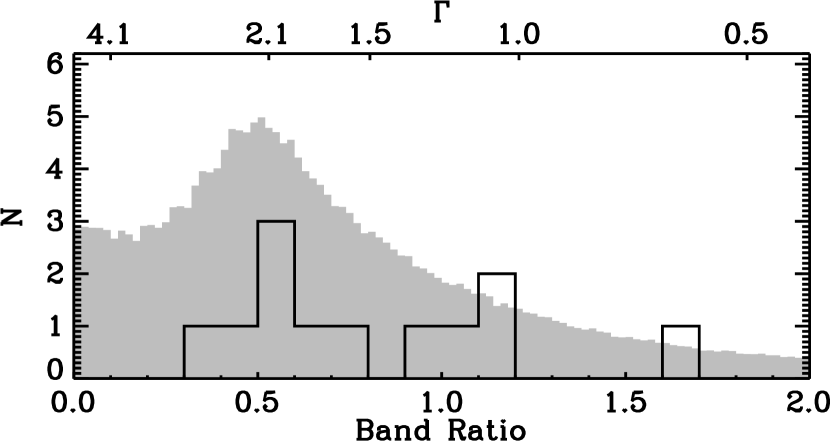
Figure 8.— 8-24 keV to 3-8 keV band ratio (bottom axis) and $\Gamma$ (top axis) distributions for our sample of “blind” sources. The solid lines indicate the distribution of sources that pass our significance threshold in both bands after deblending. The grey shaded histograms show the distribution resulting from a Monte Carlo analyses of all 49 sources that pass our significance cut in at least one band after deblending, incorporating the uncertainties on the individual band ratios and photon indices (see §3.1).

The distributions of source count rates in each of our bands are plotted in Figure 7. Here, we include all 49 significant sources, irrespective of their S/N based on our 30″ photometry measurement. The number of significant sources peaks at $\sim 0.2~{}{\rm ks^{-1}}$, $\sim 0.1~{}{\rm ks^{-1}}$ and $\sim 0.3~{}{\rm ks^{-1}}$ in the 3-8 keV, 8-24 keV and 3-24 keV bands, respectively. The lowest number of deblended net source counts in each band are 38, 37 and 36 in the 3-8 keV, 8-24 keV and 3-24 keV band, respectively, and correspond to two separate sources (NuSTAR J033121-2757.8 [source ID 2 in our table] has the lowest number of counts in the 3-8 keV band, whereas NuSTAR J033144-2803.0 [ID: 8] has the lowest number of counts in both the 8-24 keV and 3-24 keV bands etc.). Conversely, the highest net source counts in each band are 365, 197 and 545, respectively, and do correspond to the same source (NuSTAR J530642-2741.0 [ID: 29]).

Figure 8 shows the distribution of 8-24 keV to 3-8 keV band ratios for all sources that pass our significance threshold (post-deblending) in both the 8-24 keV and 3-8 keV bands. Shown on the top axis of this plot is the corresponding $\Gamma$ value. As the range of band ratios is sparsely sampled, it is difficult to interpret from the significant sources alone where the band ratio distribution of our detected sources peaks. Further insight into the distribution of band ratios for all our detected sources can be gained by taking a Monte Carlo approach to account for uncertainties in their count rates. We generate $10^{4}$ mock band ratios for each detection by randomly sampling the band ratio probability density profiles output by the BEHR code. The resulting band ratio distribution is shown in grey in 8 behind the histogram of those sources significantly detected in both bands and peaks at $\sim 0.5$, corresponding to $\Gamma\sim 2.1$. We stress that this distribution only samples the detected sources and may not be representative of the underlying band ratio distribution of the entire AGN population, which may be probed using more advanced techniques that are beyond the scope of this work (e.g., stacking on the positions of known AGN populations from, e.g., Chandra observations).

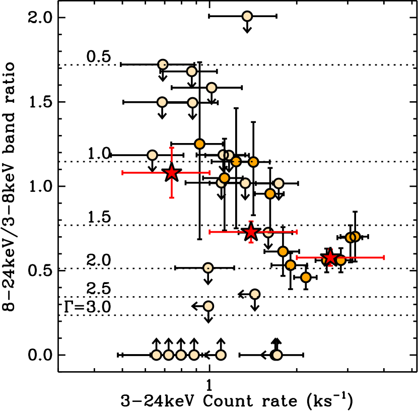
Figure 9.— 8-24 keV to 3-8 keV band ratio plotted against the aperture-corrected 3-24 keV band count rates of our detected sources. The average band ratios in three separate bins of 3-24 keV band count rate, calculated by summing the counts from all sources in each bin to obtain a stacked detection in each band, are shown as red stars. Horizontal dotted lines indicate the photon index at various band ratios.

Previous studies of deep X-ray surveys have reported an anti-correlation between the band ratio and count rate in the lower energy bands (i.e., 2-8 keV to 0.5-2 keV vs. 0.5-8 keV count rates) for AGN-dominated sources (e.g., della Ceca et al. 1999; Ueda et al. 1999; Mushotzky et al. 2000; Tozzi et al. 2001; Alexander et al. 2003). This trend has been attributed to an increase in the number of absorbed AGNs detected at lower count rates. To investigate whether we see such a trend in the NuSTAR data we plot the 8-24 keV to 3-8 keV band ratio as a function of 3-24 keV count rate in 9. The 12 sources that are detected at $>3\sigma$ in both the 8-24 keV and 3-8 keV bands appear to show a weak trend toward higher band ratios at low 3-24 keV count rates. However, the large number of sources with upper limits in either band and the narrow dynamical range in 3-24 keV count rates of those sources detected in all three bands makes it difficult to assess the significance of this trend. To investigate this possible trend, we determine average count rates in three 3-24 keV count rate bins, i.e., $0.5\leq R_{\rm FB}/{\rm ks^{-1}}<1$, $1\leq R_{\rm FB}/{\rm ks^{-1}}<2$, $2\leq R_{\rm FB}/{\rm ks^{-1}}<4$, getting $>3\sigma$ average count rates for all bands in each bin. The results of this averaging is shown in Figure 9 and shows some evidence of a decreasing hardness ratio with increasing 3-24 keV count rate, supporting previous claims from studies of lower energy X-ray bands. However, we stress that this new result is only based on three count rate bins and confirmation will be needed by extending the dynamical range in average count rates via, e.g., stacking the NuSTAR undetected population, which will be the focus of a future study (e.g., Hickox et al. in prep.).

Figure 10.— Distributions of aperture-corrected fluxes in our three bands for the sources in the “blind” catalog. Here, we only include the 49 sources that pass our significance threshold post-deblending.

In the electronic catalog, we also provide derived properties for each of our detected sources, namely the photon index, $\Gamma$, and the observed flux in each band (i.e., not corrected for absorption). The twelve sources that pass our significance thresholds in both the 8-24 keV and 3-8 keV bands cover a wide range of observed (i.e., uncorrected) photon indices, ranging from $0.51^{+0.89}_{-0.24}$ to $2.27^{+0.47}_{-0.37}$ ($1\sigma$ errors; see Figure 8). The majority (i.e., 7 of 12) of sources in our sample for which we can constrain a photon index have $\Gamma<1.8$ (i.e., the typically assumed intrinsic AGN photon index), suggesting that a large fraction of the sources have significant obscuration causing the observed photon index to harden. The median photon index and $\pm 1\sigma$ interval for these twelve sources is $\overline{\Gamma}=1.70\pm 0.52$. We use the same Monte Carlo simulations as described earlier in this section (i.e., those used to incorporate uncertainties in the band ratio distribution) to calculate the median photon index all sources, including those not individually detected in both bands, finding a somewhat softer $\overline{\Gamma}=1.90\pm 0.53$.

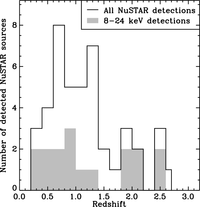
Figure 11.— Redshift distribution of the 44 NuSTAR sources that are significantly detected (post-deblending) in at least one band and have either an associated spectroscopic or photometric redshift (solid line). The shaded histogram shows the same for the 17 sources significantly detected (post-deblending) in the 8-24 keV band that have either a spectroscopic or photometric redshift.

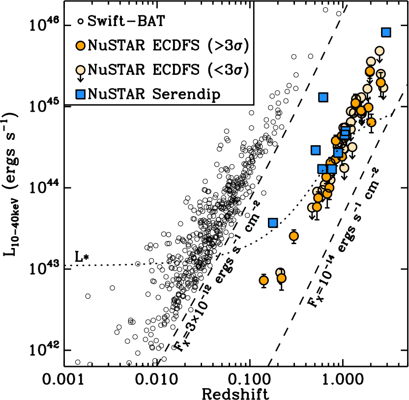
Figure 12.— X-ray luminosity in the rest-frame 10-40 keV band versus redshift for several hard X-ray selected samples. We show the NuSTAR-ECDFS sources (i.e., our sample), the first ten sources from the NuSTAR serendipitous survey (Alexander et al. 2013) and the sources from the Swift-BAT survey (Baumgartner et al. 2013). In the case of the NuSTAR-ECDFS sources, the 10-40 keV luminosity is derived from the observed 8-24 keV flux, assuming either the measured photon index ($\Gamma$) if the source is significantly detected in both the 3-8 keV and 8-24 keV bands or $\Gamma=1.8$ otherwise. Upper limits are shown for NuSTAR-ECDFS sources when the measured flux in the 8-24 keV band is $<3\sigma$. The dotted line indicates the evolution of the position of the knee of the X-ray luminosity function, extrapolated from the 2-10 keV luminosity functions of Aird et al. (2010) assuming $\Gamma=1.8$. The NuSTAR sources in the ECDFS probe to this “knee” out to $z\sim 1$.

In Figure 10 we plot the distribution of fluxes of our detected sources in each of the three bands. The faintest sources in the 3-8 keV, 8-24 keV and 3-24 keV bands have fluxes of $(8.3\pm 3.6)\times 10^{-15}$, $(2.2\pm 1.3)\times 10^{-14}$ and $(1.59\pm 0.84)\times 10^{-14}~{}{\rm ergs~{}s^{-1}~{}cm^{-2}}$, respectively, giving an indication of the approximate ultimate sensitivity limit of the survey in these bands. However, while passing our significance thresholds, these sources all have flux measurements below $3\sigma$. The faintest sources with $>3\sigma$ flux measurements have fluxes of $(1.22\pm 0.40)\times 10^{-15}$, $(3.4\pm 1.1)\times 10^{-14}$ and $(2.36\pm 0.74)\times 10^{-14}~{}{\rm ergs~{}s^{-1}~{}cm^{-2}}$ in the 3-8 keV, 8-24 keV and 3-24 keV bands, respectively. The 8-24 keV and 3-24 keV band flux limits are roughly 2 orders of magnitude fainter than those of the most sensitive observations of the Swift-BAT all-sky survey (Baumgartner et al. 2013), the previous deepest hard X-ray survey prior to the launch of NuSTAR. We note that the flux limit of the ECDFS survey is comparable to that of the six deepest observations that make up the NuSTAR Serendipitous survey (Alexander et al. 2013), although the ECDFS survey reaches this depth over a larger contiguous area and benefits from more comprehensive ancillary multiwavelength data, an aspect that is exploited in the next subsection.

The 44 sources in our sample with known redshifts span the redshift range $z=0.22-2.7$. The 10-40 keV luminosity range of the 19 of these 44 that are significantly detected in the 8-24 keV band (from which we calculated 10-40 keV luminosities) span the range $\sim 8\times 10^{42}~{}{\rm ergs~{}s^{-1}}$ to $\sim 3\times 10^{45}~{}{\rm ergs~{}s^{-1}}$. The redshift-luminosity plane for our sample, together with comparison samples from the Swift-BAT survey (Baumgartner et al. 2013) and the NuSTAR serendipitous survey (Alexander et al. 2013) is shown in 12 and highlights the complementary regions of parameter space that these various surveys cover, which is the focus of the following subsection.

3.2. Comparison with low-z samples

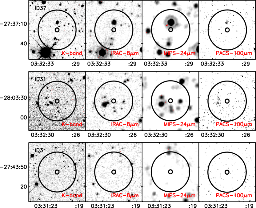
Figure 13.— Thumbnail images of the 90″$\times$90″ patches of sky at various wavelengths centered on the three NuSTAR sources without Chandra or XMM-Newton counterparts. The smaller 3″-radius circle is used to indicate the location of the NuSTAR source, while the larger circle shows the 30″ search radius we use when identifying counterparts at other wavelengths. The data used to create these images come from TENIS (K-band; Hsieh et al. 2012), SIMPLE (Spitzer-IRAC 8 ${\rm\mu m}$ $[$ i.e., Ch. 4$]$; Damen et al. 2011), FIDEL (Spitzer-MIPS 24 ${\rm\mu m}$) and PEP (Herschel-PACS; Lutz et al. 2011) surveys. Only one of these, NuSTAR -ID: 37 shows any evidence of hosting an AGN at any wavelength other than hard X-rays, which comes from mid to far-infrared SED fitting (see Figure 14).

The AGNs detected and characterized as part of the all-sky Swift-BAT survey form the local sample that is most directly comparable to the NuSTAR-ECDFS AGNs reported here. Figure 12 shows that, while the range in luminosities of both samples are large (i.e., each spanning roughly 3 orders of magnitude or more) and there is some overlap, the AGNs in the ECDFS survey are typically an order of magnitude more luminous than those in the Swift-BAT sample. As expected, the difference in the redshift distributions of the two samples is also large, with the ECDFS sample centered around $z\sim 1$, compared to $z\sim 0.03$ for the Swift-BAT sample.

To help place the two samples in a cosmological context, we include a line in 12 showing the evolution in the position of the knee (i.e., $L\ast$) of the AGN luminosity function (converted to 10-40 keV from the 2-10 keV luminosity functions of Aird et al. 2010 assuming an intrinsic photon index of $\Gamma=1.8$). The position of the two samples relative to this line demonstrates the complementary nature of these samples, with the Swift-BAT sample probing the knee of the luminosity function at $z\sim 0.015$ and the ECDFS sample probing it at $z\sim 0.8-1$. Crucially, this means that due to the evolution of the SMBH accretion rate density, the power of NuSTAR and Swift-BAT combined will enable us to probe roughly 25% of the accretion rate density of the Universe with hard X-rays, compared to just 0.5% with Swift-BAT alone.

4. NuSTAR sources without Chandra or XMM-Newton counterparts

One of NuSTAR’s primary science goals is the characterization of the sources that make up the hard (i.e., $>10$ keV) X-ray background. As such, any sources that have not previously been identified at softer X-ray energies are potentially of great interest. In this subsection, we focus on the three NuSTAR sources in the ECDFS field that we have identified as having neither Chandra nor XMM-Newton counterparts. By the definition of our detection threshold we should expect, on average, one false source per band. As such, it is plausible that all three of these NuSTAR sources with neither Chandra nor XMM-Newton counterparts are spurious. That said, it is important that we first determine whether any of these three show any other evidence of nuclear activity before rejecting them as spurious as, if confirmed, they may provide further insight into the population of Compton-thick AGNs at high redshift.

The three NuSTAR sources without Chandra or XMM-Newton counterparts are NuSTAR J033122-2743.9, NuSTAR J033228-2803.5 and NuSTAR J033231-2737.3 (hereafter, referred to by their indices in our source catalogue, i.e., 3, 31, and 37, respectively). These three sources represent $\sim 6\%$ of the total sample of the 49 NuSTAR sources that are significant post-deblending. We checked by eye the (5 and 10-pixel Gaussian-smoothed) 2-8 keV Chandra images of the ECDFS near the positions of these three NuSTAR sources, but find no indication of any weak sources that may have been missed by the source detection algorithm used in analyzing the Chandra data (see L05). We note that two of the three sources is significantly detected in only one of our three NuSTAR bands: one in the 8-24 keV band (ID: 3) and one in the 3-24 keV band (ID: 31). The third (ID: 37) is detected in both the 3-8 keV and 3-24 keV bands. Furthermore, two of these sources have $>3\sigma$ deblended fluxes in at least one band (which coincides with the band in which it is significantly detected), the exception being ID 37. Due to their faintness, all but one of these three new X-ray sources have poorly constrained photon indices, the exception being ID: 31, for which BEHR gives a (median) band ratio of $0.87^{+0.38}_{-0.45}$, corresponding to a photon index of $\Gamma=1.3^{+1.0}_{-0.3}$.

We next explore whether any of the three new X-ray sources have counterparts displaying signs of nuclear activity at wavelengths aside from X-rays (see Figure 13 for 90″$\times$90″ postage-stamp images of the regions around the NuSTAR sources in the K-band, Spitzer-IRAC Ch. 4 and MIPS-24 ${\rm\mu m}$ bands and Herschel-PACS 100 ${\rm\mu m}$ bands). We first consider the near to mid-infrared regime (specifically Spitzer’s IRAC channels), as this has been shown to be efficient at identifying highly obscured AGNs (e.g., Lacy et al. 2004; Stern et al. 2005; Donley et al. 2007, 2012). Furthermore, considering that $\approx 94\%$ of Chandra sources in the ECDFS have counterparts in at least one of the Spitzer-IRAC channels (based on a 3″ matching to the SIMPLE catalog described in Damen et al. 2011), it is highly likely that any genuine NuSTAR source will also have a Spitzer-IRAC counterpart. Indeed, with an on-sky source density of $\sim 50$ IRAC sources per arcmin², the challenge becomes identifying which, if any, of the $\sim 40$ IRAC sources within our 30″ search radius around the NuSTAR positions is the true counterpart (see Figure 13). To address this, we explore whether any of the potential counterparts display a rising power-law distribution of IRAC fluxes, which is evidence of AGN-heated dust (e.g., Donley et al. 2007, 2012). Considering the IRAC color criteria of Donley et al. (2012), which are optimized for deep IRAC data unlike the shallow-data criteria of Lacy et al. (2004) and Stern et al. (2005), none of the 95 potential IRAC counterparts show clear evidence of nuclear activity based on IRAC data.

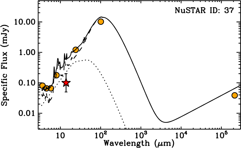
Figure 14.— Infrared spectral energy distribution for NuSTAR-ID: 37. Orange circles show data from Spitzer-IRAC, MIPS, Herschel-PACS and radio data from Bonzini et al. (2012). On fitting the infrared spectral energy distribution of this source using the AGN (dotted line) and host-galaxy (solid line) templates described in Del Moro et al. (2013), we find that an AGN component is required at a significance of $\gg 99$%. The red star shows the mid-infrared flux derived from the NuSTAR 3-8 keV flux using Eqn. 2 of Gandhi et al. (2009), which is broadly consistent with the AGN component required by the SED fit.

As IRAC power-law selection will identify only those AGN whose mid-infrared emission strongly dominates over that from star-formation, we also exploit mid to far-infrared SED fitting to identify potential infrared signatures of AGN. To get broader wavelength coverage for our SED fitting we match to Spitzer-MIPS (i.e., the FIDEL catalog; P.I.: M. Dickinson) and Herschel-PACS data (i.e., the PEP catalog; Lutz et al. 2011; Magnelli et al. 2013), matching to the positions of the potential Spitzer-IRAC counterparts identified above with a search radius of 3″. Of the 95 potential IRAC counterparts, only two have detections at 24 ${\rm\mu m}$ and at either 100 ${\rm\mu m}$ or 160 ${\rm\mu m}$ (our infrared SED fitting require at least one detection in either of the Herschel-PACS bands). The two potential far-infrared counterparts correspond to NuSTAR sources 31 and 37 (FIDEL catalog IDs: 1294 and 14000; PEP source names: PEPPRI J033229.3-280329 and PEPPRI J033231.2-273707; and redshifts of $z=0.204$ and 0.125 from the MUSYC catalog described in Cardamone et al. 2010, respectively), while NuSTAR source 3 does not have a significant far-infrared counterpart. Following Mullaney et al. (2011) we fit the infrared SEDs of these two potential counterparts, using the extended AGN and host galaxy templates of Del Moro et al. (2013). While the counterpart to NuSTAR source 31 shows no evidence of an AGN component, the counterpart to NuSTAR source 37 requires a significant AGN contribution to fit the infrared SED (required at $\gg 99\%$ significance; see Figure 14). Furthermore, converting the NuSTAR 3-8 keV flux to a 2-10 keV luminosity (assuming $\Gamma=1.8$ and $z=0.125$), and using Eqn. 2 from Gandhi et al. (2009) gives a predicted mid-infrared flux broadly consistent with the AGN contribution required by the SED fit, further strengthening the case that this is a genuine AGN. Interestingly, the SED fit also provides an explanation as to why the Spitzer-IRAC fluxes do not display a power-law distribution, with Figure 14 showing that the SED is likely dominated by emission from the host galaxy at all infrared wavelengths (e.g., Cardamone et al. 2008).

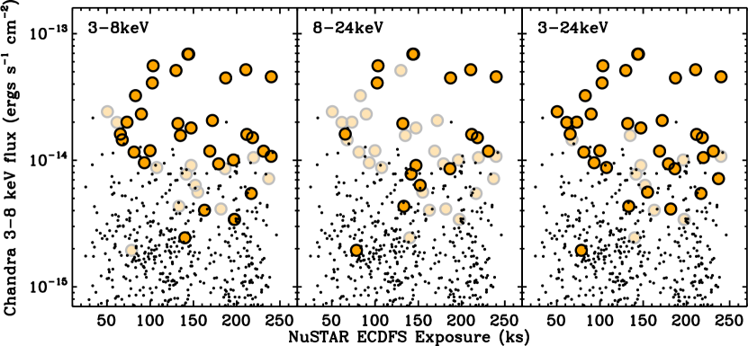
Figure 15.— Chandra-derived 3-8 keV fluxes for sources in the L05 catalog plotted against the NuSTAR exposure time at those positions (small black points). In each panel, we highlight those sources that are detected in the 3-8 keV, 8-24 keV and 3-24 keV bands (orange points). Lighter points show sources that are detected by NuSTAR but not in that specific band. As expected, NuSTAR typically detects the brightest sources at a given exposure time, although there are examples of undetected sources interspersed between the detected sources, suggesting that NuSTAR detection is not a simple function of source flux and exposure. Reasons for this are explored in §5

Finally, following Del Moro et al. (2013), we search for potential radio counterparts to the three NuSTAR sources without Chandra or XMM-Newton matches. Matching to the Bonzini et al. (2012) catalog of radio sources in the ECDFS using a 3″ search radius around the IRAC positions, we find that the two potential far-infrared counterparts identified above are also detected at 1.4 GHz (i.e., matched to NuSTAR sources 31 and 37). As these sources are detected at far-infrared wavelengths, we explore whether either show a radio excess above that predicted by the far-infrared/radio correlation that could indicate the presence of an obscured AGN. However, we find that the radio fluxes are consistent with star-formation in both cases (see Figure 14 for the infrared to radio SED of NuSTAR ID: 37) .

To summarize this section, we detect three NuSTAR sources that have neither Chandra nor XMM-Newton counterparts. From the definition of our detection threshold we expect 2-3 of these to be spurious (i.e., due to random noise fluctuations). Analysis of the infrared SEDs of potential counterparts reveals some evidence that one of these NuSTAR sources (ID: 37) displays excess flux at mid-infrared wavelengths that may be attributable to an obscured AGN. However, no evidence of this AGN is seen at near-infrared wavelengths (i.e., via power-law Spitzer-IRAC fluxes) or radio frequencies (i.e., via a radio excess). Further evidence of an obscured AGN in these systems may be identified via other techniques, such as via their rest-frame optical spectra (i.e., BPT diagnostics; Baldwin et al. 1981), although we note that the most heavily obscured can still be missed using these methods (e.g., Stern et al. 2014). However, at present, such spectra are are unavailable for the potential counterparts identified here.

5. The NuSTAR-detected population in the context of the Chandra-ECDFS source population

As we have seen, the majority of our significantly detected NuSTAR sources have Chandra counterparts. In this section, we consider how the NuSTAR-detected population relates to the wider population of X-ray sources previously detected in the Chandra ECDFS survey. First, to explore whether the Chandra flux is a strong predictor of whether a source is detected by NuSTAR (as would be expected), we first plot the distribution of Chandra 3-8 keV fluxes for each source in the L05 catalog against the mean NuSTAR exposure time at that position, highlighting those that are detected in each of our three NuSTAR bands (i.e., 3-8 keV, 8-24 keV, 3-24 keV; see Figure 15). This plot indeed shows that the brightest Chandra sources are preferentially detected by NuSTAR, with 24 of the 34 sources (i.e., $71\%$) with Chandra-measured $F_{\rm 3-8~{}keV}>10^{-14}~{}{\rm ergs~{}s^{-1}~{}cm^{-2}}$ and NuSTAR exposure $>50~{}{\rm ks}$ detected in at least one NuSTAR band. Of the other ten, four seem to be associated with local minima in the $P_{\rm False}$ maps that lie just above our detection threshold (i.e., having ${\rm log}(P_{\rm False})>-4.5$, compared to our threshold of $\sim-5.2$). Thus, while formally undetected, there is at least some evidence of their presence in the NuSTAR maps. By contrast, there is no hint of a reduced $P_{\rm False}$ in the NuSTAR maps at the positions of the other six bright Chandra sources. Five of these lie in regions of the NuSTAR maps with comparatively low exposure (i.e., $<100$ ks), which may explain their non-detection. One, however, lies in a region of relatively high exposure (i.e., $\sim 190$ ks; L05-ID: 577) and thus, with a Chandra 3-8 keV flux of $2\times 10^{-14}~{}{\rm ergs~{}s^{-1}~{}cm^{-2}}$ and a photon index of 1.67, we would expect it to be detected by NuSTAR. One possibility for the lack of NuSTAR detection is source variability, with a factor of a $\sim$few reduction in flux being sufficient to explain the lack of detection. However, with similar fluxes between the Chandra and XMM-Newton observations (separated by $\sim 8$ years), this source shows little evidence of strong variability. As such, at present it is not clear why the bright Chandra source L05: 577 is not detected by NuSTAR.

Comparing between the individual bands in Figure 15, it is evident that the relationship between the Chandra 3-8 keV flux and NuSTAR detection differs between the NuSTAR bands. As expected, detection in the NuSTAR 3-8 keV band is strongly related to the Chandra 3-8 keV flux, with the vast majority of the detections (i.e., 25 of 33) in this band having Chandra-measured $F_{\rm 3-8~{}keV}>10^{-14}~{}{\rm ergs~{}s^{-1}~{}cm^{-2}}$. However, this correspondence between detection and Chandra flux is weaker in the 8-24 keV band, with only 11 of the 37 Chandra sources with Chandra-measured $F_{\rm 3-8~{}keV}>10^{-14}~{}{\rm ergs~{}s^{-1}~{}cm^{-2}}$ being detected in this harder band. Interestingly, the source with the faintest Chandra 3-8 keV counterpart of all the NuSTAR sources is detected in the 8-24 keV NuSTAR band, but not the 3-8 keV band (NuSTAR J033144-2803.0; NuSTAR-ECDFS ID: 8; L05 ID: 145). A NuSTAR detection in the 8-24 keV band, but not the 3-8 keV band, indicates a hard X-ray photon index, but with a Chandra-measured photon index of $\Gamma=1.51$ for this source, this does not appear to be the case. Again, we checked for possible counterparts in the later XMM-Newton observations of the field, but found none (i.e., it is undetected in the XMM-Newton 2-10 keV band), so we are unable to rule out source variability as an explanation for the NuSTAR detection of this comparatively faint Chandra source. We do note, however, that the next faintest Chandra source detected in the NuSTAR 8-24 keV band does have a very hard Chandra-derived photon index of $\Gamma=-0.72$ (NuSTAR J033145-2745.2; NuSTAR-ECDFS ID: 9; L05 ID: 152), which would explain its strong detection in this band.

In light of this faint, but very hard photon index Chandra source being detected with NuSTAR, we explore what bearing the Chandra-derived hardness ratio (i.e., the 2-8 keV to 0.5-2 keV ratio) has on NuSTAR detections in general. For this, we plot the Chandra-derived hardness ratio against Chandra-derived 3-8 keV fluxes for sources detected in the ECDFS survey (L05), highlighting those that are detected by NuSTAR (see Figure 16). Here, we only plot sources with $>50$ ks of NuSTAR coverage. For those NuSTAR sources with multiple Chandra counterparts we plot the hardness ratio derived from summing the 2-8 keV to 0.5-2 keV band counts from all counterparts and the sum of their 3-8 keV fluxes. From this plot, there is no strong evidence that sources detected in the NuSTAR 8-24 keV band are preferentially those with harder X-ray spectra (based on Chandra hardness ratios). Indeed, the majority (i.e., five of eight) of sources detected in NuSTAR 8-24 keV band but not the 3-8 keV band have a hardness ratio below the median value for all Chandra ECDFS sources (i.e., 0.85). This also holds for all NuSTAR sources detected in the 8-24 keV band, not just those that are not also detected at 3-8 keV (i.e., 15 of 22 have hardness ratios below the median value). As such, based on this analysis, we find no strong evidence that the Chandra hardness ratio has a strong bearing on whether a source is detected by NuSTAR, although we acknowledge our relatively small sample size. Source variability may be able to explain some of this effect, although another possibility is that simple Chandra hardness ratios are a poor proxy for the true spectral properties of the X-ray sources detected by NuSTAR. Ascertaining whether this is indeed the case will be the focus of future papers exploring the spectral properties of these NuSTAR sources in detail.

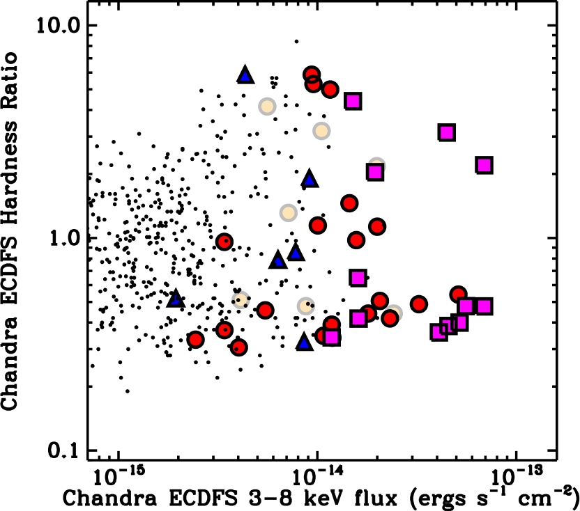
Figure 16.— Plot of Chandra-derived 2-8 keV/0.5-2 keV hardness ratio against Chandra-measured 3-8 keV flux for detected Chandra sources in the ECDFS (small points). Highlighted are those sources that are detected by NuSTAR in the 3-8 keV band but not the 8-24 keV band (red circles), those that are detected in the 8-24 keV band but not the 3-8 keV band (blue triangles), those that are detected in both the 3-8 keV and 8-24 keV bands (magenta squares), and those that are only detected in the single 3-24 keV band (faint circles). For those NuSTAR sources with multiple Chandra counterparts we plot the hardness ratio derived from summing the 2-8 keV to 0.5-2 keV band counts from all counterparts and the sum of their 3-8 keV fluxes. While there is a clear tendency for the NuSTAR-detected sources tend to be the brightest Chandra sources, as expected, there is not clear connection between Chandra-derived hardness ratio and whether a source is detected by NuSTAR at 8-24 keV.

6. Summary

In this paper we have described the NuSTAR survey of the ECDFS and presented the first results from considering the population of sources detected by NuSTAR in this field. Such blank field surveys are a crucial first step in determining the number counts (i.e., logN-logS) and luminosity function of the resolved hard X-ray (i.e., $>8~{}{\rm keV}$) source population, which will be the focus of two future papers (Harrison et al. in prep. and Aird et al. in prep., respectively). With a maximum unvignetted exposure of $\approx 360$ ks, the ECDFS currently represents the deepest contiguous component of the NuSTAR extragalactic survey, reaching sensitivity limits of $\approx 1.3\times 10^{-14}~{}{\rm ergs~{}s^{-1}~{}cm^{-2}}$ (3-8 keV), $\approx 3.4\times 10^{-14}~{}{\rm ergs~{}s^{-1}~{}cm^{-2}}$ (8-24 keV) and $\approx 3.0\times 10^{-14}~{}{\rm ergs~{}s^{-1}~{}cm^{-2}}$ (3-24 keV). Our main results from this first paper looking at the population of NuSTAR sources detected in the ECDFS can be summarized as:

• within the full $\sim 30\arcmin\times 30\arcmin$ ECDFS, we detect 54 NuSTAR sources, although only 49 of these remain significant after the effects of neighboring sources are taken into account (i.e., after deblending). Nineteen of these 49 are detected in the 8-24 keV band - the energy range uniquely probed by NuSTAR to unprecedented depths (see §3.1);

• twelve sources are detected in both the 3-8 keV and 8-24 keV energy bands, enabling us to determine their hardness ratios and, correspondingly, estimate their photon indices within this energy range. The twelve sources display photon indices that span a broad range of values, i.e., $\Gamma=0.5-2.3$, with a median of $\Gamma=1.70\pm 0.52$. By adopting a Monte Carlo approach to sample the band ratio probability distribution function of all 49 detected sources, we calculate the median photon index for the whole sample as $\Gamma=1.90\pm 0.53$ (see §3.1);

• all but three of the 49 significantly detected NuSTAR sources have X-ray counterparts in either the Chandra or XMM-Newton surveys of the ECDFS. The redshift of these counterparts span the range $z=0.21-2.7$ which, when combined with their NuSTAR fluxes, corresponds to a 10-40 keV luminosity range for our deblended sample of $(\approx 0.7-300)\times 10^{43}~{}{\rm ergs~{}s^{-1}}$. As such, our NuSTAR sample probes below the knee of the extrapolated X-ray luminosity function at $z<1$ (see §§3.1, 3.2);

• of the three NuSTAR sources without Chandra or XMM-Newton counterparts, only one shows evidence of AGN signatures at other wavelengths (i.e., via infrared SED fitting; see §4); and

• as expected, a high Chandra 3-8 keV flux is a good predictor as to whether a source will be detected in other NuSTAR bands. However, it is not a 1:1 correlation, with some of the brightest Chandra sources not being detected at higher energies with NuSTAR. The reason for this is currently unclear, as the Chandra- derived hardness ratio seems to have very little bearing on whether a sources is detected in a given NuSTAR band (see §5), but source variability may provide some explanation.

We thank the anonymous referee for their careful reading of the manuscript and comments which improved the clarity of the text. This work made use of data from the NuSTAR mission, a project led by the California Institute of Technology, managed by the Jet Propulsion Laboratory, and funded by the National Aeronautics and Space Administration. We thank the NuSTAR Operations, Software and Calibration teams for support with the execution and analysis of these observations. This research has made use of the NuSTAR Data Analysis Software (NUSTARDAS) jointly developed by the ASI Science Data Center (ASDC, Italy) and the California Institute of Technology (USA). ADM and DMA gratefully acknowledge financial support from the Science and Technology Facilities Council (ST/I001573/1). JA acknowledges support from a COFUND Junior Research Fellowship from the Institute of Advanced Study, Durham University, and ERC Advanced Grant FEEDBACK at the University of Cambridge. FMC acknowledges support from NASA grants 11-ADAP11-0218 and GO3-14150C. DRB is supported in part by NSF award AST 1008067. WNB and BL thank NuSTAR grant 44A-1092750, NASA ADP grant NNX10AC99G, and the V. M. Willaman Endowment. We acknowledge support from CONICYT-Chile grants Basal-CATA PFB-06/2007 (FEB), FONDECYT 1141218 (FEB) and 1120061 (ET), and ”EMBIGGEN” Anillo ACT1101 (FEB, ET); the Ministry of Economy, Development, and Tourism’s Millennium Science Initiative through grant IC120009, awarded to The Millennium Institute of Astrophysics, MAS (FEB). Support for the work of ET was also provided by the Center of Excellence in Astrophysics and Associated Technologies (PFB 06). AC, SP and LZ acknowledge support from the ASI/INAF grant I/037/12/0– 011/13. AC acknowledges the Caltech Kingsley visitor program. M. B. acknowledges support from NASA Headquarters under the NASA Earth and Space Science Fellowship Program, grant NNX14AQ07H.

Appendix A Catalog Description

Table 3Overview of Columns in the NuSTAR ECDFS Source Catalog

Column	Description
1	Unique NuSTAR ECDFS survey source identification number
2	Name of NuSTAR source
3, 4	Right ascention and declination of the NuSTAR source
5-7	Flag indicating in which of the three standard bands the source is detected
8-10	Flag indicating in which of the three standard bands the source is detected post deblending.
11-14	Logarithm of the undeblended false probability in the three standard bands
15-16	Logarithm of the deblended false probability in the three standard bands
17	Flag indicating whether the source remains significant post-deblending
18-32	Total, background and net source counts and associated errors in the three standard bands
33-44	Deblended total, background and net sources counts and associated errors in the three standard bands
45-47	Effective exposure times for the three standard bands
48-62	Total, background and net source count rates and associated errors in the three standard bands
63-68	Deblended total, background and net source count rates and associated errors in the three standard bands
69-73	Band ratio; mean, median, mode and upper and lower limits returned by BEHR algorithm
74-76	Effective photon index and upper and lower limits
77-82	Derived fluxes in the three standard bands
83-88	Derived deblended fluxes in the three standard bands
89	Counterpart catalogue code (L05: Lehmer et al. 2005; R13: Ranalli et al. 2013, X11: Xue et al. 2011)
90	Unique identification number of the associated source in the counterpart catalogue
91, 92	Right ascention and declination of the associated in the counterpart catalogue
93	Separation between the NuSTAR position and the associated source in the counterpart catalogue
94	3-8 keV Chandra or XMM-Newton flux of the associated source in the counterpart catalogue
95	Combined 3-8 keV or Chandra or XMM-Newton flux of all associated sources within 30″ of the NuSTAR position
96	Spectroscopic redshift of the associated source in the counterpart catalogue
97	Photometric redshift of the associated source in the counterpart catalogue
98	Adopted redshift
99, 100	Non-absorption-corrected rest-frame 10-40keV luminosity and associated error of the NuSTAR source
101	Source notes.

The final catalog of 54 sources generated using the procedure outlined above is available in the form of an electronic table. A summary of the columns of this table is given in Table 3, which we expand upon here:

Column 1: The unique NuSTAR ECDFS identification number. Sources are arranged in right-ascention order. Multiple rows labelled with the same identifier correspond to where one NuSTAR source is matched to more than one Chandra source within 30″.

Column 2: The unique name of the NuSTAR source, following the IAU-approved naming convention for NuSTAR sources: NuSTAR JHHMMSS$\pm$DDMM.m, where m is the truncated fraction of an arcminute in declination for the arcseconds component.

Columns 3,4: The right ascention and declination of the NuSTAR source. The position is that of the pixel with the lowest $P_{\rm False}$ in the 20″-smoothed maps across all bands. The position is taken from the band showing the lowest $P_{\rm False}$ (i.e., the band in which the source is most significantly detected). All following photometry etc. is then performed at this one position in all three bands.

Columns 5-7: Binary flag indicating in which of the three standard bands the source is formally detected (i.e., meets our final thresholds of ${\rm log}(P_{\rm False})\leq-5.19,\leq-5.22$ and $\leq-5.34$ in the 3-8 keV, 8-24 keV and 3-24 keV bands, respectively). Here, and throughout the table, the 3-8 keV, 8-24 keV and 3-24 keV bands are abbreviated to SB, HB and FB, respectively.

Columns 8-10: The same as columns 5-7, but after photon counts from neighboring sources have been excluded (i.e., deblending; see §2.3.2).

Columns 11-13: The logarithm of $P_{\rm False}$ (i.e., ${\rm log}(P_{\rm False})$) in each of the three standard bands based on a 20″ smoothing length, i.e., the smoothing length adopted to assess whether a source is significantly detected (see §2.3.1).

Columns 14-16: The same as columns 11-13, but after photon counts from neighboring sources have been excluded (i.e., deblending; see §2.3.2).

Column 17: Binary flag indicating whether the NuSTAR source remains significant in at least one of the standard bands post-deblending.

Columns 18-32: Non-aperture-corrected total, background and net source counts based on 30″ aperture photometry centered on the position in columns 3,4 in each of the three standard bands. Errors are given on the total and net counts and are calculated using Gehrels (1986) (see §2.3.2). We indicate those sources where the photometric measurement in a given band is $<3\sigma$ with a negative value for the error.

Columns 33-44: Same as columns 18-32, but after source counts from neighboring sources have been taken into account (still based on 30″ aperture photometry). Errors are given on the net counts.

Columns 45-47: Mean effective exposure times in 30″ apertures centered on the position in columns 3,4 in each of the three standard bands. Unit: s.

Columns 48-62: Non-aperture-corrected total, background and net source count rates, calculated from the source counts in columns 18-32 and the respective mean effective exposure times in columns 45-47). Errors are propagated from those on the source counts, assuming zero error on the effective exposure times. Again, negative error values indicate those sources that are detected at $<3\sigma$ in a given band. Unit: ${\rm s^{-1}}$.

Columns 63-68: Same as columns 48-62, but after the effects of source blending has been taken into account (i.e., calculated using the source counts given in columns 33-44 and respective mean effective exposure times given in columns 45-47). Unit: ${\rm s^{-1}}$.

Columns 69-73: 8-24 keV to 3-8 keV band ratios output by the BEHR algorithm. As this algorithm is a Bayesian Estimator, it calculates the band ratio probability distribution function and provides the mean, median, mode and upper and lower 68th percentiles, which we report here.

Columns 74-76: Effective observed (i.e., non-absorption-corrected) photon index of the NuSTAR source derived from the mean band ratio and the upper and lower limits given in columns 69-73 (see §2.3.3).

Columns 77-82: Observed-frame, aperture corrected source fluxes in the three standard bands. Fluxes are derived from net count rates (columns 48-62) following the procedure outlined in §2.3.3. Errors are propagated using the same conversion factors. Again, negative error values indicate those sources that are detected at $<3\sigma$ in a given band. Units: ${\rm ergs~{}s^{-1}~{}cm^{-2}}$

Columns 83-88: Same as columns 77-82, but after the effects of source blending have been taken into account (i.e., using the deblended count-rates in columns 63-68).

Columns 89: Code indicating the catalog in which a Chandra or XMM-Newton counterpart to the NuSTAR source was identified. L05: Lehmer et al. (2005); R13: Ranalli et al. (2013); X11: Xue et al. (2011).

Column 90: unique identifier of the matched Chandra Chandra or XMM-Newton source(s) from the catalog indicated in column 89 (“recno” in the L05 and X11 catalogs; “ID210” in the R13 catalog) . Where there are more than one match within 30″ of the NuSTAR position, we provide separate matches on additional table rows. Such multiple matches can therefore be identified by the replication of the NuSTAR index in column 1.

Columns 91,92: Right-ascention and declination of the respective Chandra or XMM-Newton match(es).

Column 93: Separation between the NuSTAR source and the matched Chandra or XMM-Newton source. Unit: arcsecond.

Column 94: Observed-frame 3-8 keV fluxes derived from the Chandra or XMM-Newton data. Note: these data are not provided in the catalogs of L05, Ranalli et al. (2013) or Xue et al. (2011) as the 3-8 keV band is not a standard band of those papers. Instead, the 3-8 keV fluxes were calculated using ACIS Extract (Broos et al. 2010) with a simple power-law model. Units: ${\rm ergs~{}s^{-1}~{}cm^{-2}}$.

Column 95: Total combined observed-frame 3-8 keV fluxes of all Chandra or XMM-Newton sources within 30″ of the NuSTAR source. Units: ${\rm ergs~{}s^{-1}~{}cm^{-2}}$.

Column 96: Spectroscopic redshift of the matched Chandra (from Silverman et al. 2010 ) or XMM-Newton (from Ranalli et al. 2013) source, where available.

Column 97: Photometric redshift of the matched Chandra (from Silverman et al. 2010 ) or XMM-Newton (from Ranalli et al. 2013) source, where available.

Column 98: The adopted redshift used to calculate the rest-frame 10-40 keV luminosity of the NuSTAR source. In cases where both spectroscopic and photometric redshifts are available, we always adopt the spectroscopic redshift.

Columns 99, 100: Derived rest-frame 10-40 keV luminosities of the NuSTAR sources and associated errors for sources where a redshift is available (either photometric of spectroscopic). Luminosities are calculated using the observed 8-24 keV band flux and $k$-corrections are performed assuming a photon index of $\Gamma=1.8$ (see §2.3.4). Where a NuSTAR source is matched to more than one Chandra or XMM-Newton source (and therefore may have more than one associated redshift), we provide the 10-40 keV luminosity assuming each of the various available redshifts. Errors are propagated directly from the errors on the 8-24 keV fluxes (i.e., we assume zero error on the redshift). Again, negative error values indicate those sources that are detected at $<3\sigma$ in a given band. Units: ${\rm ergs~{}s^{-1}}$

Column 101: Any special notes associated with the source.

References

- Aird et al. (2010) Aird, J., Nandra, K., Laird, E. S., et al. 2010, MNRAS, 401, 2531
- Ajello et al. (2012) Ajello, M., Alexander, D. M., Greiner, J., et al. 2012, ApJ, 749, 21
- Ajello et al. (2008) Ajello, M., Greiner, J., Kanbach, G., et al. 2008, ApJ, 678, 102
- Akylas et al. (2012) Akylas, A., Georgakakis, A., Georgantopoulos, I., Brightman, M., & Nandra, K. 2012, A&A, 546, A98
- Alexander & Hickox (2012) Alexander, D. M., & Hickox, R. C. 2012, New Astronomy Reviews, 56, 93
- Alexander et al. (2003) Alexander, D. M., Bauer, F. E., Brandt, W. N., et al. 2003, AJ, 126, 539
- Alexander et al. (2013) Alexander, D. M., Stern, D., Del Moro, A., et al. 2013, ApJ, 773, 125
- Baldwin et al. (1981) Baldwin, J. A., Phillips, M. M., & Terlevich, R. 1981, PASP, 93, 5
- Ballantyne (2014) Ballantyne, D. R. 2014, MNRAS, 437, 2845
- Ballantyne et al. (2011) Ballantyne, D. R., Draper, A. R., Madsen, K. K., Rigby, J. R., & Treister, E. 2011, ApJ, 736, 56
- Ballantyne et al. (2006) Ballantyne, D. R., Everett, J. E., & Murray, N. 2006, ApJ, 639, 740
- Baumgartner et al. (2013) Baumgartner, W. H., Tueller, J., Markwardt, C. B., et al. 2013, ApJS, 207, 19
- Bertin & Arnouts (1996) Bertin, E., & Arnouts, S. 1996, A&AS, 117, 393
- Bonzini et al. (2012) Bonzini, M., Mainieri, V., Padovani, P., et al. 2012, ApJS, 203, 15
- Bottacini et al. (2012) Bottacini, E., Ajello, M., & Greiner, J. 2012, ApJS, 201, 34
- Brandt & Alexander (2015) Brandt, W. N., & Alexander, D. M. 2015, A&A Rev., 23, 1
- Broos et al. (2010) Broos, P. S., Townsley, L. K., Feigelson, E. D., et al. 2010, ApJ, 714, 1582
- Brusa et al. (2009) Brusa, M., Comastri, A., Gilli, R., et al. 2009, ApJ, 693, 8
- Burlon et al. (2011) Burlon, D., Ajello, M., Greiner, J., et al. 2011, ApJ, 728, 58
- Cardamone et al. (2008) Cardamone, C. N., Urry, C. M., Damen, M., et al. 2008, ApJ, 680, 130
- Cardamone et al. (2010) Cardamone, C. N., van Dokkum, P. G., Urry, C. M., et al. 2010, ApJS, 189, 270
- Churazov et al. (2007) Churazov, E., Sunyaev, R., Revnivtsev, M., et al. 2007, A&A, 467, 529
- Civano et al. (submitted) Civano, F., Hickox, R. C., Puccetti, S., et al., submitted to ApJ
- Civano et al. (2012) Civano, F., Elvis, M., Brusa, M., et al. 2012, ApJS, 201, 30
- Comastri et al. (1995) Comastri, A., Setti, G., Zamorani, G., & Hasinger, G. 1995, A&A, 296, 1
- Damen et al. (2011) Damen, M., Labbé, I., van Dokkum, P. G., et al. 2011, ApJ, 727, 1
- Del Moro et al. (2013) Del Moro, A., Alexander, D. M., Mullaney, J. R., et al. 2013, A&A, 549, A59
- Del Moro et al. (2014) Del Moro, A., Mullaney, J. R., Alexander, D. M., et al. 2014, ApJ, 786, 16
- della Ceca et al. (1999) della Ceca, R., Castelli, G., Braito, V., Cagnoni, I., & Maccacaro, T. 1999, ApJ, 524, 674
- Donley et al. (2007) Donley, J. L., Rieke, G. H., Pérez-González, P. G., Rigby, J. R., & Alonso-Herrero, A. 2007, ApJ, 660, 167
- Donley et al. (2012) Donley, J. L., Koekemoer, A. M., Brusa, M., et al. 2012, ApJ, 748, 142
- Elvis et al. (2009) Elvis, M., Civano, F., Vignali, C., et al. 2009, ApJS, 184, 158
- Freeman et al. (2002) Freeman, P. E., Kashyap, V., Rosner, R., & Lamb, D. Q. 2002, ApJS, 138, 185
- Frontera et al. (2007) Frontera, F., Orlandini, M., Landi, R., et al. 2007, ApJ, 666, 86
- Gandhi et al. (2009) Gandhi, P., Horst, H., Smette, A., et al. 2009, A&A, 502, 457
- Gehrels (1986) Gehrels, N. 1986, ApJ, 303, 336
- Georgakakis et al. (2008) Georgakakis, A., Nandra, K., Laird, E. S., Aird, J., & Trichas, M. 2008, MNRAS, 388, 1205
- Giacconi et al. (1962) Giacconi, R., Gursky, H., Paolini, F. R., & Rossi, B. B. 1962, Physical Review Letters, 9, 439
- Gilli et al. (2007) Gilli, R., Comastri, A., & Hasinger, G. 2007, A&A, 463, 79
- Gilli et al. (2001) Gilli, R., Salvati, M., & Hasinger, G. 2001, A&A, 366, 407
- Goulding et al. (2012) Goulding, A. D., Forman, W. R., Hickox, R. C., et al. 2012, ApJS, 202, 6
- Gruber et al. (1999) Gruber, D. E., Matteson, J. L., Peterson, L. E., & Jung, G. V. 1999, ApJ, 520, 124
- Harrison et al. (2013) Harrison, F. A., Craig, W. W., Christensen, F. E., et al. 2013, ApJ, 770, 103
- Hasinger (2008) Hasinger, G. 2008, A&A, 490, 905
- Hickox & Markevitch (2006) Hickox, R. C., & Markevitch, M. 2006, ApJ, 645, 95
- Hsieh et al. (2012) Hsieh, B.-C., Wang, W.-H., Hsieh, C.-C., et al. 2012, ApJS, 203, 23
- Krivonos et al. (2007) Krivonos, R., Revnivtsev, M., Lutovinov, A., et al. 2007, A&A, 475, 775
- Lacy et al. (2004) Lacy, M., Storrie-Lombardi, L. J., Sajina, A., et al. 2004, ApJS, 154, 166
- Laird et al. (2009) Laird, E. S., Nandra, K., Georgakakis, A., et al. 2009, ApJS, 180, 102
- Lehmer et al. (2005) Lehmer, B. D., Brandt, W. N., Alexander, D. M., et al. 2005, ApJS, 161, 21
- Lehmer et al. (2012) Lehmer, B. D., Xue, Y. Q., Brandt, W. N., et al. 2012, ApJ, 752, 46
- Luo et al. (2008) Luo, B., Bauer, F. E., Brandt, W. N., et al. 2008, ApJS, 179, 19
- Lutz et al. (2011) Lutz, D., Poglitsch, A., Altieri, B., et al. 2011, A&A, 532, A90
- Madau et al. (1994) Madau, P., Ghisellini, G., & Fabian, A. C. 1994, MNRAS, 270, L17
- Magnelli et al. (2013) Magnelli, B., Popesso, P., Berta, S., et al. 2013, A&A, 553, A132
- Marshall et al. (1980) Marshall, F. E., Boldt, E. A., Holt, S. S., et al. 1980, ApJ, 235, 4
- Mullaney et al. (2011) Mullaney, J. R., Alexander, D. M., Goulding, A. D., & Hickox, R. C. 2011, MNRAS, 414, 1082
- Mushotzky et al. (2000) Mushotzky, R. F., Cowie, L. L., Barger, A. J., & Arnaud, K. A. 2000, Nature, 404, 459
- Paolillo et al. (2004) Paolillo, M., Schreier, E. J., Giacconi, R., Koekemoer, A. M., & Grogin, N. A. 2004, ApJ, 611, 93
- Park et al. (2006) Park, T., Kashyap, V. L., Siemiginowska, A., et al. 2006, ApJ, 652, 610
- Ranalli et al. (2013) Ranalli, P., Comastri, A., Vignali, C., et al. 2013, A&A, 555, A42
- Scoville et al. (2007) Scoville, N., Aussel, H., Brusa, M., et al. 2007, ApJS, 172, 1
- Setti & Woltjer (1989) Setti, G., & Woltjer, L. 1989, A&A, 224, L21
- Silverman et al. (2010) Silverman, J. D., Mainieri, V., Salvato, M., et al. 2010, ApJS, 191, 124
- Stern et al. (2005) Stern, D., Eisenhardt, P., Gorjian, V., et al. 2005, ApJ, 631, 163
- Stern et al. (2014) Stern, D., Lansbury, G. B., Assef, R. J., et al. 2014, ApJ, 794, 102
- Tomsick et al. (2014) Tomsick, J. A., Gotthelf, E. V., Rahoui, F., et al. 2014, ApJ, 785, 4
- Tozzi et al. (2001) Tozzi, P., Rosati, P., Nonino, M., et al. 2001, ApJ, 562, 42
- Treister & Urry (2005) Treister, E., & Urry, C. M. 2005, ApJ, 630, 115
- Treister et al. (2009) Treister, E., Urry, C. M., & Virani, S. 2009, ApJ, 696, 110
- Tueller et al. (2008) Tueller, J., Mushotzky, R. F., Barthelmy, S., et al. 2008, ApJ, 681, 113
- Ueda et al. (2014) Ueda, Y., Akiyama, M., Hasinger, G., Miyaji, T., & Watson, M. G. 2014, ApJ, 786, 104
- Ueda et al. (1999) Ueda, Y., Takahashi, T., Inoue, H., et al. 1999, ApJ, 518, 656
- Vasudevan et al. (2013) Vasudevan, R. V., Mushotzky, R. F., & Gandhi, P. 2013, ApJ, 770, L37
- Wik et al. (2014) Wik, D. R., Hornstrup, A., Molendi, S., et al. 2014, ApJ, 792, 48
- Worsley et al. (2005) Worsley, M. A., Fabian, A. C., Bauer, F. E., et al. 2005, MNRAS, 357, 1281
- Xue et al. (2011) Xue, Y. Q., Luo, B., Brandt, W. N., et al. 2011, ApJS, 195, 10
- Xue et al. (2012) Xue, Y. Q., Wang, S. X., Brandt, W. N., et al. 2012, ApJ, 758, 129
- Young et al. (2012) Young, M., Brandt, W. N., Xue, Y. Q., et al. 2012, ApJ, 748, 124