Quantifying Quantum Resource Sharing

Abstract

Entanglement is a key resource of quantum science for tasks that require it to be shared among participants. Within atomic, condensed matter and photonic many-body systems the distribution and sharing of entanglement is of particular importance for information processing by progressively larger and larger quantum networks. Here we report a singly-bipartitioned qubit entanglement inequality that applies to any N-party qubit pure state and is completely tight. It provides the first prescription for a direct calculation of the amount of entanglement sharing that is possible among N qubit parties. A geometric representation of the measure is easily visualized via polytopes within entanglement hypercubes.

Introduction: Resource sharing is a concern everywhere in science and technology, as well as in everyday life. It always becomes harder to allocate resources if there are more recipients, and is still harder if there are complicated restrictions on the allocations. These obvious considerations can become acute when the resource has specific or even uniquely valuable qualities. A prime example of this is many-body quantum entanglement Horodecki-etal-09 , a property of quantum systems that is not only desirable but necessary in order to capture quantum advantages in applications such as randomness generation Pironio-etal-10 , cryptography Gisin-etal-02 , computing Nielsen-Chuang-00 and network formation Kimble-08 . Despite the long-recognized value of entanglement, it has remained unknown how to determine either the kind or amount of qubit entanglement present in an arbitrary many-body solid state, atomic or photonic system Vidal-00 . More particularly, the ways that quantum restrictions affect sharing between or among units in the system have remained mysterious. A key obstacle is the inability to recognize, much less catalog, all restrictions. These are open issues affecting, for example, multi-electron atomic ionization Becker-etal-12 , multilevel coding for quantum key distribution Multi-QKD and multiparty teleportation MultiParty-tele ; MultiEnt-tele .

An early advance more than a decade ago used concurrence Wootters-98 as the entanglement measure to identify the concept of quantum monogamy (see Coffman, et al. Coffman-etal-00 ). As applied to three qubits it demonstrated sharing or additivity by proving that the squared concurrence of qubit $A$, with qubits $B$ and $C$ being considered as a unit, must be greater than or equal to the sum of squared concurrences of $A$ with $B$, and $A$ with $C$, when $B$ and $C$ are considered separately. The positive difference is known to serve as a three-body entanglement monotone DVC-00 . The monogamy proof is symmetric and generic, applying to any three-qubit pure state, and each qubit is allowed to arrange its two states arbitrarily. A series of extensions Osborne-Verstraete-06 ; Lohmayer-etal-06 ; Ou-Fan-07 ; Hiroshima-etal-07 ; Eltschka-etal-09 ; Giorgi-11 ; Streltsov-etal-12 ; Bai-etal-14 ; Regula-etal-14 have shown that the monogamy inequality continues to hold for $N$-qubit states. So far, in no case has sharing been quantified.

We have been exploring Qian-Eberly-10 ; Qian-etal-14 influences on quantum interactions arising from poorly known or hidden background parties, i.e., many-body quantum systems that have unspecified entanglements, both among themselves and with a designated qubit of interest. We here report one of the consequences, the discovery of a generic and completely tight inequality among one-party marginal qubit entanglements, a symmetric linear relation restricting the entanglements of each qubit with all of the others. It is an inequality that applies to every qubit of any particle type in an arbitrary many-body pure-state qubit system. As a consequence, we can report a quantitative prescription for the amount of sharing that is possible of such entanglements. A laboratory examination of entanglement dynamics reported earlier Brazil and based on an incomplete version Qian-Eberly-10 of the new entanglement inequality, suggests that it will be experimentally accessible.

N-Party Entanglement Sharing: An arbitrarily entangled $N$-qubit pure state is written

$$|\Psi_{1,2,...,N}\rangle=\sum_{s_{1},...,s_{N}=0,1}c_{s_{1},...,s_{N}}|s_{1}\rangle...|s_{N}\rangle,$$ (1)

where $c_{s_{1},...,s_{N}}$ are normalized coefficients and $s_{j}$ takes values 0 or 1 corresponding to the two states $|0\rangle$, $|1\rangle$ of the $j$-th qubit, with $j=1,2,3,...,N$. In this $N$-qubit system, we compute the degree of entanglement of any one qubit (as one party) with the remaining qubits (as the other party). Under such a bipartition, the pure state (1) above can always be decomposed into Schmidt form Schmidt ; Fedorov-Miklin-14 ; Ekert-Knight-95 , a sum of only two terms because the singled-out qubit itself has only two states, i.e.,

$$|\Psi_{1,2,...,N}\rangle=\sum_{n=1}^{2}\sqrt{\lambda_{n}^{(j)}}|f_{n}^{(j)}\rangle\otimes|g_{n}^{(j)}\rangle,$$ (2)

where $|f_{n}^{(j)}\rangle$ and $|g_{n}^{(j)}\rangle$ are the “information eigenstates” of the reduced density matrices of the $j$-th qubit and the remaining $N-1$ qubits, from whose joint state the Schmidt Theorem Schmidt determines the unique two-dimensional partner of the $j$-th qubit. The Schmidt coefficients $\lambda_{1}^{(j)}$ and $\lambda_{2}^{(j)}$ are the corresponding eigenvalues of the reduced density matrix for one party, i.e., the single-qubit, and are the same for both parties.

The degree of entanglement between the $j$-th qubit and the remaining $N-1$ qubits can be characterized in a number of ways, frequently by the Schmidt weight $K_{j}$, which is given in K : $1/K_{j}=(\lambda_{1}^{(j)})^{2}+(\lambda_{2}^{(j)})^{2}$. For our purposes an alternate normalized form is more useful:

$$Y_{j}=1-\sqrt{2/K_{j}-1},$$ (3)

which can also be recognized as two times the smaller of $\lambda^{(j)}_{1}$ and $\lambda^{(j)}_{2}$. Thus this entanglement monotone satisfies $0\leq Y_{j}\leq 1$, where 0 indicates complete separability (zero entanglement), and 1 denotes maximal entanglement.

Our first main result for this entanglement measure is a compact generic and symmetric entanglement inequality applying to all the $Y_{j}$ values for the $N$ qubits:

$$Y_{j}\leq\sum_{k\neq j}Y_{k}.$$ (4)

The proof of inequality (4) is lengthy and is given in the supplementary material Suppl.Matl. . One notes that the inequality takes a form that is available to other N-party entanglement monotones, such as the von Neumann entropy and concurrence which are concave functions of $Y$. However, most importantly, inequality (4) is uniquely tight. In fact, the concavity of other entanglement monotones with respect to $Y$ already indicates a looser form of inequality than (4). By saying uniquely tight, it means that (4) not only applies to all $N$-party qubit pure states, but additionally that those states exhaust the inequality, occupying its interior and also its boundaries. We will develop this point in the following sections. An interesting trivial consequence is obtained immediately by adding $Y_{j}$ to both sides of (4), to get the total $Y_{T}$ of all one-party marginal entanglements on the right side. Thus no arbitrarily chosen $j$-th member of the party can capture more than half of the total $Y_{T}$. This is independent of the way the $N$-body state is specified.

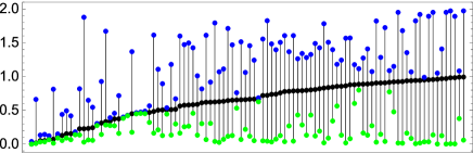
Figure 1: Illustration of upper and lower bounds of $Y_{1}$. Black dots indicate the $Y_{1}$ values for 100 randomly chosen 3-qubit pure states. The blue (upper) dots identify each state’s upper bound determined from (4) and the connected green (lower) dots identify the lower bound obtained from (7) as converted from the monogamy relation (5).

Connection to Monogamy: The constraints provided by our inequality (4) are different from those of the well-known monogamy relations Coffman-etal-00 ; Osborne-Verstraete-06 . However, a direct comparison can be made with the $j$-th concurrence, the one analogous to $Y_{j}$, i.e., based on the same bipartitioning. The Osborne-Verstraete proof Osborne-Verstraete-06 of the $N$-qubit version of the concurrence relation reads

$$C^{2}_{j\{N-1\}}\geq\sum_{k\neq j}C^{2}_{jk}.$$ (5)

Here we denote $C_{jk}$ as the concurrence of parties $j$ and $k$ and, as in (4), the right-hand sum includes the other $N-1$ qubits entangled with qubit $j$. On the left side of the inequality $C_{j\{N-1\}}$ denotes the concurrence of $j$ with the other $N-1$ qubits which, taken together, have been reduced to single-qubit form by the Schmidt Theorem Schmidt . When applied to arbitrary $N$-qubit pure states, $C_{j\{N-1\}}$ is a simple concave function of $Y_{j}$ in [0,1]:

$$C_{j\{N-1\}}^{2}=Y_{j}(2-Y_{j}).$$ (6)

This converts to an inequality by substitution from (5) and we find

$$Y_{j}\geq 1-\sqrt{1-\sum_{k\neq j}C^{2}_{jk}}.$$ (7)

This specifies a lower bound for $Y_{j}$ to accompany the upper bound $\sum_{k\neq j}Y_{k}$ that is provided by our basic inequality (4). To give a concrete view of the new result, these upper and lower bounds are shown in Fig. 1 for 100 random three-qubit pure states. Notice that for some states the upper and lower bounds almost coincide, indicating a similar tightness of the two opposite bounds. A more precise upper bound of $Y_{j}$ would be ${\rm Min}[1,\sum_{k\neq j}Y_{k}]$ since all $Y_{k}$ are less than 1. This will simply bring all the higher upper bound points down to 1.

Polytope Analysis: We now present our second main result. We first exploit the $N$ different $Y_{j}$ measures by using them to identify axes in a unit $N$-dimensional space. All possible $N$-dimensional vectors ${\bf Y}=(Y_{1},Y_{2},...,Y_{N})$ live inside a unit $N$-dimensional hypercube, since $0\leq Y_{j}\leq 1$. For $N=3$, for example, ${\bf Y}$ is a three-dimensional vector inside the unit cube, shown in Fig. 2(c). The cube’s origin $(0,0,0)$ represents zero entanglement (corresponding to completely separable states), while the opposite corner $(1,1,1)$ represents maximal entanglement and corresponds to a GHZ state GHZ-07 . It is worth stressing that ${\bf Y}$ is invariant to unitary local transformations of the state. The new inequality (4) implies that the region inhabitable by the vectors ${\bf Y}$ (for pure states) is more restricted than the $N$-dimensional unit hypercube.

Our second result is that these relations define a polytope, a hypervolume that is compact inside the unit hypercube, where all possible ${\bf Y}$ are located. This polytope geometrically represents the entanglement inequalities (4). Each inequality excludes a rectangular simplex whose hypervolume is given by:

$$\prod_{j=1}^{N}\int_{0}^{1}[Y_{j}]^{j-1}dY_{j}=\frac{1}{N!}.$$ (8)

Therefore the total available hypervolume, given the restrictions by all $N$ such inequalities, is

$$V_{N}=1-\frac{1}{(N-1)!}.$$ (9)

To begin to visualize the effect of these constraints, we consider the case $N=2$.

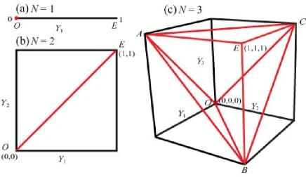
Figure 2: $N$-dimensional spaces in which the vector ${\bf Y}$ is defined, corresponding to (a) $N=1$ (unit line segment), (b) $N=2$ (unit square), and (c) $N=3$ (unit cube). In all cases, the point $O$ corresponds to no entanglement and the point $E$ to maximal entanglement.

For $N=2$ there are two axes, $Y_{1}$ and $Y_{2}$, and their joint range is the unit square shown in Fig. 2(b). In this case the inequalities (4) are simply $Y_{1}\geq Y_{2}$ and $Y_{2}\geq Y_{1}$, or $Y_{1}=Y_{2}$. This restricts the allowed region to a single line inside the unit square (dotted line in Fig. 2(b)) running along the diagonal. On this line the total entanglement $Y_{T}=Y_{1}+Y_{2}$ runs from 0 to 2, from the completely separable point $O$ to the maximally entangled point $E$ (corresponding to a Bell state). We note that for $N=2$ entanglement can’t be additively shared. The only way for $Y_{1}$ and $Y_{2}$ to add up to any given $Y_{T}$ is $Y_{1}=Y_{2}=\frac{1}{2}Y_{T}$. Again, this agrees with Eq. (9) – the restricted volume fraction is $V_{2}=0$, meaning that instead of an area, only a line is inhabitable. The even simpler case $N=1$ restricts occupation to a single point, $Y_{1}=0$.

In the case $N=3$ additive sharing first comes into play. The three entanglements $Y_{1},\ Y_{2},\ Y_{3}$ now reside inside a unit cube (see Fig. 2(c)). From (4) the generic three qubit inequalities are given as

$$Y_{1}+Y_{2}\geq Y_{3},\quad Y_{2}+Y_{3}\geq Y_{1},\quad Y_{3}+Y_{1}\geq Y_{2}.$$ (10)

One notes that when the three relations are equalities, each of them defines a surface of the regular tetrahedron $OABC$. That is, the three equilateral triangles $\triangle OAB$, $\triangle OBC$, and $\triangle OCA$ are the surfaces separating allowed and forbidden regions, as shown in Fig. 3. Combining this with the fact that $Y_{1},Y_{2},Y_{3}\leq 1$, the inhabitable region resulting from the constraints by the three inequalities is simply the base-to-base union of the regular tetrahedron $OABC$ and the rectangular tetrahedron $ABCE$. This combined region is shown, shaded in gray, in Fig. 3. There are now many ways for the three entaglements to add to a given total $Y_{T}$, and sharing is discussed in the following section. As specified by Eq. (9), the restricted volume is $V_{3}=1/2$. That is, only half of the cube is inhabitable by pure three-qubit states.

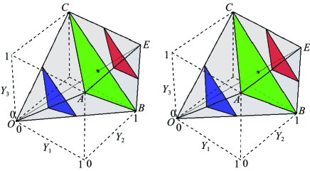
Figure 3: Stereogram best viewed from a distance of about 25 cm. It shows the inhabitable region of the 3D cube permitted by the inequalities (4), i.e., the polyhedron $OABCE$ (shaded in gray). See also Movie 1 Suppl.Matl. . Also shown are three triangular planar sections of this region transverse to the unit cube’s body diagonal. See also Movie 2 Suppl.Matl. .

Let us now view these results in regard to the well-known generalized GHZ GHZ-07 and inequivalent W DVC-00 classes of three-qubit states:

$$|\Psi_{\rm GHZ}\rangle=\cos\theta|0,0,0\rangle+\sin\theta|1,1,1\rangle,$$ (11)

and

$$|\Psi_{\rm W}\rangle=\alpha|1,0,0\rangle+\beta|0,1,0\rangle+\gamma|0,0,1\rangle.$$ (12)

It is straightforward to find that the GHZ states and their arbitrary local unitary transformations live along the cube’s body diagonal line $OE$ (see Fig. 3), according to $Y_{1}=Y_{2}=Y_{3}=1-|\cos 2\theta|$. The W class of states and their local unitary transformations, on the other hand, live on the four surfaces of the regular tetrahedron, i.e., $\triangle ABC$ as well as the inequality boundaries $\triangle OAB$, $\triangle OBC$, and $\triangle OCA$. The occupation of these boundaries indicates the unique tightness of our inequalities (4). The W class states all live away from the diagonal line $OE$ except for the three trivial cases when only one of $\alpha,\beta,\gamma$ is nonzero, and one non-trivial case for the perfectly symmetric W state when $|\alpha|=|\beta|=|\gamma|=1/\sqrt{3}$. This state and the surface $\triangle ABC$, which is the common base of the two tetrahedra, have a special character that will be discussed in the following section.

For $N\geq 3$, the inequalities are simultaneously all equalities only if all the $Y_{j}$ vanish.

For $N\geq 4$ qubits, the available region for all $Y_{j}$ is an $N$-dimensional hypercube, and the allowed region, restricted by Eq. (4), is an $N$-dimensional convex polytope. According to Eq. (9), the ratio of the allowed region $V_{N}$ to the unit hypervolume increases as the number of qubits is increased, approaching unity as $N\to\infty$. This can be understood as a consequence of multi-party entanglement because the entanglement information shared among a higher number of parties is less restricted than for a lower number.

Entanglement Additivity: The geometric representation provided by the ${\bf Y}$-space in the three-qubit case helps visualize how entanglement inequalities provide a natural measure of sharing or additivity, the freedom to distribute individual entanglements in a way that the sum adds to a given $Y_{T}$. We start by noticing that the domains of different total entanglements $Y_{T}$ define triangles transverse to the body diagonal (color triangles in Fig. 3). Inspection shows that the $Y_{T}$ value for these triangles varies from 0 to 3, running from zero to maximal total entanglement. It is obvious that many combinations of the $Y_{j}$ are available to sum to the total $Y_{T}$ in each transverse triangle.

Our third main result is to adopt the area of each triangle to serve as a natural measure of this entanglement additivity, which we denote by ${\cal A}$. This interpretation is also natural for $N=1$ and $N=2$. In those cases ${\cal A}=0$ because the counterparts of the transverse triangles are simply zero-area points, corresponding to the lack of alternative arrangements of the individual $Y_{j}$. The relation between ${\cal A}$ and the amount of entanglement to be shared is not a linear relation, but a piece-wise quadratic of the form:

$${\cal A} = \frac{\sqrt{3}}{2}\times\left\{\begin{array}[]{cc}Y_{T}^{2}/4,&0\leq Y_{T}\leq 2,\\ (3-Y_{T})^{2},&2\leq Y_{T}\leq 3.\end{array}\right.$$ (15)

The additivity ${\cal A}$ is graphed for $N=3$ in Fig. 4, where we see that it is peaked around its maximum of $\sqrt{3}/2$ at $Y_{\rm T}=2$, corresponding to the triangle $\triangle ABC$. Clearly, more total entanglement $Y_{T}$ does not guarantee greater additivity.

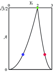
Figure 4: Additivity ${\cal A}$ is shown as a function of $Y_{\rm T}$. The three colored dots correspond respectively to the three colored triangles in Fig. 3.

Note that the triangle joining the tetrahedral bases and shown in green in Fig. 3, has a special character. It contains all of the W states in Eq. (12) that satisfy ${\rm Max}(|\alpha|^{2},\ |\beta|^{2},\ |\gamma|^{2})\leq 1/2$; and the perfectly symmetric W state lives at the point where the cube’s body diagonal $OE$ intersects the triangle. Thus W-like states can exhibit maximum additive entanglement sharing. At the apexes $O$ and $E$, corresponding to $Y_{\rm T}=0$ and $Y_{\rm T}=3$, respectively, the transverse triangles have zero area. This is intuitively correct since neither zero entanglement nor full total entanglement can be distributed in any different way. In contrast to the W state, one also notes that for any given $Y_{T}$, each GHZ-like state is a single point on the body diagonal line $OE$ and so it permits zero sharing (${\cal A}=0$).

One can easily extend the above analysis to the $N$-qubit case, where additivity is then defined as the hyperarea of the $(N-1)$-dimensional inhabitable polytope of fixed $Y_{\rm T}$, normal to the line $OE$ within the $N$-dimensional polytope restricted by the $N$ inequalities (4). This expression is given by a piecewise polynomial of $Y_{\rm T}$ of order $N-1$, which vanishes at the endpoints $Y_{\rm T}=0$ (corresponding to point $O$) and $Y_{\rm T}=N$ (corresponding to point $E$).

Summary: Our results bring new light to the understanding of quantum multiparty entanglement by focusing on the simplest form of many-body bi-partitioning. This leads to the emergence of the uniquely tight new quantum many-body inequality (4) that applies to each of the one-party marginal entanglement monotones $Y_{j}$ defined in (3), as proved in Suppl.Matl. . It provides a compact expression for the restrictions that are acting, and they act in the opposite sense of monogamy, as demonstrated in Fig. 1. Thus they illuminate a new aspect of generic resource sharing different from that represented by monogamy.

Our inequalities provide an improved view of pure-state entanglement and not only impose new quantum many-body limits on one-party marginal entanglement, but also allow the sharing of entanglement among members of an arbitrary many-body pure qubit state to be quantified. They allow, we believe, the first quantitative definition of additivity ${\cal A}$, a measure of the extent to which the individual entanglements $Y_{j}$ can be added to produce a prescribed total $Y_{T}$. One consequence is that more entanglement resource does not necessarily mean greater additivity. This is obviously applicable to tasks when optimum sharing instead of maximum entanglement is to be emphasized.

We have shown that all of the consequences of the inequality (4), and the character of the additivity measure ${\cal A}$, can be associated with the surfaces and volumes of allowed vector spaces within hypercubes. These polytopes are illustrated for $N=3$ in Fig. 3. The simplicity of our approach is a key to our results. Preliminary numerical results support the speculation that the same inequalities of $Y_{j}$ hold for pure states of many-body $M$-level systems, where the normalized entanglement monotone becomes $Y_{j}=1-\sqrt{\frac{M/K_{j}-1}{M-1}}$. This may supply a route for discovery of additional resource-sharing equalities that may be based on inequalities reported for quantum marginal multiparticle entanglement by Walter, et al., Walter-etal-13 for higher dimensional systems than qubits.

As will be discussed elsewhere, our entanglement inequality (4) for pure states remains relevant to mixed-state generalizations. Then the inhabitable regions of the hypercube are different. Dynamical trajectories within the allowed polytopes are also under investigation, as well as alternative interpretations of the ${\bf Y}$ space.

Acknowledgement: We acknowledge partial financial support from the National Science Foundation through awards PHY-0855701, PHY-1068325, PHY-1203931, PHY-1505189, and INSPIRE PHY-1539859.

References

- (1) See R. Horodecki, P. Horodecki, M. Horodecki and K. Horodecki, Rev. Mod. Phys. 81, 865-942 (2009).
- (2) See S. Pironio, A. Acin, S. Massar, et al., Nature 464, 1021 (2010).
- (3) See N. Gisin, G. Ribordy, W. Tittel, and H. Zbinden, Rev. Mod. Phys. 74, 145 (2002).
- (4) See Quantum Computation and Quantum Information, by M.A. Nielsen and I.L. Chuang (Cambridge Univ. Press, 2000).
- (5) See for example an overview by, H.J. Kimble, Nature 453, 1023 (2008).
- (6) For a thorough overview, see G. Vidal, J. Mod. Opt. 47, 335 (2000).
- (7) See W. Becker, X.J. Liu, P.J. Ho, et al., Rev. Mod. Phys. 84 1011 (2012).
- (8) M. Bourennane, A. Karlsson, and G. Björk, Phys. Rev. A 64, 012306 (2001).
- (9) F.-G. Deng, C.-Y. Li, Y.-S. Li, H.-Y. Zhou, and Y. Wang, Phys. Rev. A 72, 022338 (2005).
- (10) P.-X. Chen, S.-Y. Zhu, and G.-C. Guo, Phys. Rev. A 74, 032324 (2006).
- (11) W. K. Wootters, Phys. Rev. Lett. 80, 2245 (1998).
- (12) V. Coffman, J. Kundu, and W. K. Wootters, Phys. Rev. A 61, 052306 (2000).
- (13) W. Dür, G. Vidal, and J.I. Cirac, Phys. Rev. A 62, 062314 (2000).
- (14) T.J. Osborne and F. Verstraete, Phys. Rev. Lett. 96, 220503 (2006).
- (15) R. Lohmayer, A. Osterloh, J. Siewert, and A. Uhlmann, Phys. Rev. Lett. 97, 260502 (2006).
- (16) Y.-C. Ou and H. Fan, Phys. Rev. A 75, 062308 (2007).
- (17) T. Hiroshima, G. Adesso, and F. Illuminati, Phys. Rev. Lett. 98, 050503 (2007).
- (18) G. L. Giorgi, Phys. Rev. A 84, 054301 (2011).
- (19) A. Streltsov, G. Adesso, M. Piani, and D. Brüß, Phys. Rev. Lett. 109, 050503 (2012).
- (20) Y.-K. Bai, Y.-F. Xu, and Z. D. Wang, Phys. Rev. Lett. 113, 100503 (2014).
- (21) C. Eltschka, A. Osterloh and J. Siewert, Phys. Rev. A 80, 032313 (2009).
- (22) B. Regula, S. D. Martino, S. Lee, and G. Adesso, Phys. Rev. Lett. 113, 110501 (2014).
- (23) See X.-F. Qian and J.H. Eberly, arXiv: 1009.5622 (2010), and X.-F. Qian, Effect of Non-interacting Quantum Background on Entanglement Dynamics, PhD thesis, University of Rochester (2014).
- (24) X.-F. Qian, C.J. Broadbent and J.H. Eberly, New J. Phys. 16, 013033 (2014).
- (25) O. Jiménez Farías, et al., Phys. Rev. A 85, 012314 (2012).
- (26) The Schmidt theorem is the analog in analytic function theory of the singular-value decomposition theorem for matrices. The original paper is: E. Schmidt, Math. Ann. 63, 433 (1907). For background, see Fedorov and Miklin Fedorov-Miklin-14 .
- (27) M.V. Fedorov and N.I. Miklin, Contem. Phys. 55, 94 (2014).
- (28) A. Ekert and P.L. Knight, Am. J. Phys. 63, 415 (1995).
- (29) R. Grobe, K. Rza̧żewski and J. H. Eberly, J. Phys. B 27, L503 (1994).
- (30) See the supplementary material.
- (31) The original suggestion of GHZ states was given by D.M. Greenberger, M.A. Horne, and A. Zeilinger, “Going Beyond Bell’s Theorem”. See arXiv:0712.0921 (2007).
- (32) M. Walter, B. Doran, D. Gross, and M. Christandl, Science 340, 1205 (2013).