Coexistence of nuclear shapes: self-consistent mean-field and beyond

Abstract

A quantitative analysis of the evolution of nuclear shapes and shape phase transitions, including regions of short-lived nuclei that are becoming accessible in experiments at radioactive-beam facilities, necessitate accurate modeling of the underlying nucleonic dynamics. Important theoretical advances have recently been made in studies of complex shapes and the corresponding excitation spectra and electromagnetic decay patterns, especially in the “beyond mean-field” framework based on nuclear density functionals. Interesting applications include studies of shape evolution and coexistence in $N=28$ isotones, the structure of lowest $0^{+}$ excitations in deformed $N\approx 90$ rare-earth nuclei, and quadrupole and octupole shape transitions in thorium isotopes.

1 Introduction

One of the most studied phenomenon in low-energy nuclear physics, both experimentally and theoretically, is the way nucleonic matter organises itself to support a variety of shapes observed in finite nuclei. The occurrence of different shapes, shape coexistence, and shape transitions have their origin in the evolution of single-nucleon shell structure with nuclear deformation, angular momentum, temperature and number of valence nucleons. The manifestation of shells is a generic property of finite fermion systems and shell closures, in particular, are characteristic of the confining single-particle potential. When nucleons completely fill a major shell (single or doubly closed-shell nuclei), the relatively large energy gap to the next shell stabilises a spherical shape, whereas long-range correlations between valence nucleons in open-shell nuclei drive the nucleus toward deformed (quadrupole, octupole) equilibrium shapes.

Coexistence of different shapes in a single nucleus, and shape (phase) transitions as a function of nucleon number, present universal phenomena that occur in light, medium-heavy, heavy and superheavy nuclei, and reflect the organisation of nucleons in finite nuclei [1, 2, 3, 4]. A unified description of shape evolution and shape coexistence over the entire chart of nuclides necessitates a universal theory framework that can be applied to different mass regions. Nuclear energy density functionals (EDF) provide an economic, global and accurate microscopic approach to nuclear structure that can be extended from relatively light systems to superheavy nuclei, and from the valley of $\beta$-stability to the particle drip-lines [5, 6, 7, 8]. This is particularly important for extrapolations to regions far from stability where not enough data are available to determine the parameters of a more local approach such as, for instance, the interacting shell model.

The basic implementation of the EDF framework is in terms of self-consistent mean-field (SCMF) models, in which an EDF is constructed as a functional of one-body nucleon density matrices that correspond to a single product state. Nuclear SCMF models effectively map the many-body problem onto a one-body problem, and the exact EDF is approximated by simple functionals of powers and gradients of ground-state nucleon densities and currents. Some of the advantages of the EDF approach are apparent already at the SCMF level: an intuitive interpretation of mean-field results in terms of intrinsic shapes and single-nucleon states, and the possibility to formulate structure models in the full model space of occupied states, with no distinction between core and valence nucleons.

Quantitative studies of low-energy structure phenomena related to shell evolution and coexistence usually start from a constrained Hartree-Fock plus BCS (HFBCS), or Hartree-Fock-Bogoliubov (HFB) calculation of the deformation energy surfaces with mass multipole moments as constrained quantities. When based on microscopic EDFs or effective interactions, such calculations comprise many-body correlations related to the short-range repulsive inter-nucleon interaction and long-range correlations mediated by nuclear resonance modes. The result are static symmetry-breaking product many-body states. The basic idea of a deformation energy surface is that, even though the quantum many-body system is determined by a very large number of microscopic states, these can be organised in a collection of basins that are robust to small external perturbations [9]. The basins can be structurally distinct and distant from each other, but they can occur at comparable energies.

The constrained SCMF method, however, produces semi-classical deformation energy surfaces. The static nuclear mean-field is characterised by the breaking of symmetries of the underlying Hamiltonian – translational, rotational, particle number and, therefore, includes important static correlations, e.g. deformations and pairing. To calculate excitation spectra and electromagnetic transition rates it is necessary to extend the SCMF scheme to include collective correlations that arise from symmetry restoration and fluctuations around the mean-field minima. Collective correlations are sensitive to shell effects, display pronounced variations with particle number and, therefore, cannot be incorporated in a universal EDF but rather require an explicit treatment [5, 10, 11].

On the second level of implementation of nuclear EDFs that takes into account collective correlations through the restoration of broken symmetries and configuration mixing of symmetry-breaking product states, the many-body energy takes the form of a functional of all transition density matrices that can be constructed from the chosen set of product states. This set is chosen to restore symmetries or/and to perform a mixing of configurations that correspond to specific collective modes using, for instance, the (quasiparticle) random-phase approximation (QRPA) or the Generator Coordinate Method (GCM) [12]. The latter includes correlations related to finite-size fluctuations in a collective degree of freedom and presents the most effective approach for configuration mixing calculations, with multipole moments used as coordinates that generate the intrinsic wave functions.

Many interesting phenomena related to shell evolution have been investigated over the last decade by employing GCM configuration mixing of angular-momentum and particle-number projected states based on energy density functionals or effective interactions, but the extension of this method to non-axial shapes and/or heavy nuclei still presents formidable conceptual and computational challenges [11, 13, 14, 15, 16]. In an alternative approach to nuclear collective dynamics that restores rotational symmetry and allows for fluctuations around mean-field minima, a collective Hamiltonian can be formulated, with deformation-dependent parameters determined by self-consistent mean-field calculations [17, 18]. The dynamics of the collective Hamiltonian is governed by the vibrational inertial functions and the moments of inertia [19], and these functions are determined by the microscopic nuclear energy density functional and the effective interaction in the pairing channel. Five-dimensional collective Hamiltonian models for quadrupole vibrational and rotational degrees of freedom, with parameters determined by constrained triaxial SCMF calculations based on the Gogny effective interaction [20], the Skyrme density functional [18], and relativistic density functionals [10], have been developed over the last decade and applied in a number of studies of structure phenomena related to shape coexistence and shape transitions.

The present study is based on the framework of relativistic energy density functionals, extended to include the treatment of collective correlations using the collective Hamiltonian model [10]. To emphasise the universality of the EDF approach, all illustrative calculations performed in this study, from relatively light systems to very heavy nuclei, have been carried out using a single energy density functional – DD-PC1 [21]. Starting from microscopic nucleon self-energies in nuclear matter, and empirical global properties of the nuclear matter equation of state, the coupling parameters of DD-PC1 were fine-tuned to the experimental masses of a set of 64 deformed nuclei in the mass regions $A\approx 150-180$ and $A\approx 230-250$. The functional has been further tested in a number of mean-field and beyond-mean-field calculations in different mass regions. For the examples considered here, pairing correlations have been taken into account by employing an interaction that is separable in momentum space, and is completely determined by two parameters adjusted to reproduce the empirical bell-shaped pairing gap in symmetric nuclear matter [22]. For the details of the particular implementation of the EDF-based collective Hamiltonian used in the present study, we refer the reader to Ref. [10].

2 Beyond the relativistic mean-field approximation: collective correlations

For a self-consistent description of collective excitation spectra and electromagnetic transition rates, the framework of (relativistic) energy density functionals has to be extended to take into account collective correlations in relation to restoration of broken symmetries and fluctuations in collective coordinates. Both types of correlations can be included simultaneously by mixing symmetry-projected states corresponding to different values of chosen collective coordinates. The most effective approach for configuration mixing calculations is the generator coordinate method (GCM), with multipole moments used as coordinates that generate the intrinsic wave functions. The GCM is based on the assumption that, starting from a set of mean-field states $\left|\Phi(q)\right\rangle$ that depend on a collective coordinate $q$, one can build approximate eigenstates of the nuclear Hamiltonian:

$$\left|\Psi_{\alpha}\right\rangle=\int dq{f_{\alpha}(q)\left|\Phi(q)\right\rangle}\;.$$ (1)

Here the basis states $\left|\Phi(q)\right\rangle$ are Slater determinants of single-nucleon states generated by constrained SCMF calculations. Several advanced implementations of the GCM have been developed recently, fully based on the microscopic EDF framework. For the relativistic SCMF approach, in particular, the most advanced model performs configuration mixing of angular-momentum and particle-number projected wave functions generated by constraints on quadrupole deformations [15, 23]

$$|JNZ;\alpha\rangle=\int{dq\sum_{K}{f_{\alpha}^{JK}\hat{P}^{J}_{MK}\hat{P}^{N}\hat{P}^{Z}|q\rangle}},$$ (2)

where $\alpha=1,2,\dots$ denotes different collective states for a given angular momentum $J$, and $|q\rangle\equiv|\beta,\gamma\rangle$ denotes a set of intrinsic SCMF states with deformation parameters $(\beta,\gamma)$. $\hat{P}_{MK}^{J}$ is the angular momentum projection operator, and the operators $\hat{P}^{N}$ and $\hat{P}^{Z}$ project onto states with good neutron and proton number, respectively. This implementation is equivalent to a seven-dimensional GCM calculation, mixing all five degrees of freedom of the quadrupole operator and the gauge angles for protons and neutrons. The weight functions $f^{JK}_{\alpha}(q)$ in the collective wave function are determined from the variational equation:

$$\delta E^{J}=\delta\frac{\left\langle\Psi_{\alpha}^{JM}\right|\hat{H}\left|\Psi_{\alpha}^{JM}\right\rangle}{\left\langle\Psi_{\alpha}^{JM}\right|\Psi_{\alpha}^{JM}\rangle}=0\;,$$ (3)

that is, by requiring that the expectation value of the Hamiltonian is stationary with respect to an arbitrary variation $\delta f_{\alpha}^{JK}$. This leads to the Hill-Wheeler-Griffin (HWG) integral equation:

$$\int dq^{\prime}\sum_{K^{\prime}\geq 0}\left[\mathcal{H}^{J}_{KK^{\prime}}(q,q^{\prime})-E^{J}_{\alpha}\mathcal{N}^{J}_{KK^{\prime}}(q,q^{\prime})\right]f^{JK^{\prime}}_{\alpha}(q^{\prime})=0,$$ (4)

where $\mathcal{H}$ and $\mathcal{N}$ are the projected GCM kernel matrices of the Hamiltonian and the norm, respectively [13, 14, 15, 23].

Multidimensional GCM calculations involve a number of technical and computational issues [11, 23, 16], that have so far impeded systematic applications to medium-heavy and heavy nuclei. Collective dynamics can also be described using an alternative method in which a collective Hamiltonian is constructed, with deformation-dependent parameters determined from microscopic SCMF calculations [17, 18]. The collective Hamiltonian can be derived in the Gaussian overlap approximation (GOA) [12] to the full multi-dimensional GCM. With the assumption that the GCM overlap kernels can be approximated by Gaussian functions, the local expansion of the kernels up to second order in the non-locality transforms the GCM Hill-Wheeler equation into a second-order differential equation - the Schrödinger equation for the collective Hamiltonian. For instance, in the case of quadrupole degrees of freedom:

$$\hat{H}_{\rm coll}=\hat{T}_{\rm{vib}}+\hat{T}_{\rm{rot}}+V_{\rm{coll}}\;,$$ (5)

where the vibrational kinetic energy is parameterized by the the mass parameters $B_{\beta\beta}$, $B_{\beta\gamma}$, $B_{\gamma\gamma}$

$$\hat{T}_{\textnormal{vib}}=-\frac{\hbar^{2}}{2\sqrt{wr}}\left\{\frac{1}{\beta^{4}}\left[\frac{\partial}{\partial\beta}\sqrt{\frac{r}{w}}\beta^{4}B_{\gamma\gamma}\frac{\partial}{\partial\beta}-\frac{\partial}{\partial\beta}\sqrt{\frac{r}{w}}\beta^{3}B_{\beta\gamma}\frac{\partial}{\partial\gamma}\right]\right.$$

$$+\frac{1}{\beta\sin{3\gamma}}\left.\left[-\frac{\partial}{\partial\gamma}\sqrt{\frac{r}{w}}\sin{3\gamma}B_{\beta\gamma}\frac{\partial}{\partial\beta}+\frac{1}{\beta}\frac{\partial}{\partial\gamma}\sqrt{\frac{r}{w}}\sin{3\gamma}B_{\beta\beta}\frac{\partial}{\partial\gamma}\right]\right\}\;,$$ (6)

the three moments of inertia $\mathcal{I}_{k}$ determine the rotational kinetic energy

$$\hat{T}_{\textnormal{{{rot}}}}=\frac{1}{2}\sum_{k=1}^{3}{\frac{\hat{J}^{2}_{k}}{\mathcal{I}_{k}}}\;,$$ (7)

and $V_{\rm{coll}}$ is the collective potential that includes zero-point energy (ZPE) corrections. $w$ and $r$ are products of mass parameters and moments of inertia, respectively, that specify the volume element in collective space [24]. The self-consistent mean-field solution for the single-quasiparticle energies and wave functions for the entire energy surface, as functions of the quadrupole deformations $\beta$ and $\gamma$, provide the microscopic input for calculation of the mass parameters, moments of inertia and the collective potential. The Hamiltonian describes quadrupole vibrations, rotations, and the coupling of these collective modes.

The dynamics of the collective Bohr Hamiltonian is governed by the vibrational inertial functions and the moments of inertia [19]. For these quantities either the GCM-GOA or the adiabatic approximation to the time-dependent HFB (ATDHFB) expressions (Thouless-Valatin masses) can be used. The Thouless-Valatin masses have the advantage that they also include the time-odd components of the mean-field potential and, in this sense, the full dynamics of a nuclear system. In the GCM approach these components can only be included if, in addition to the coordinates $q_{i}$, the corresponding canonically conjugate momenta $p_{i}$ are also taken into account. In many applications, including the collective Hamiltonians considered in the present study, a further simplification is thus introduced in terms of cranking formulas, i.e. the perturbative limit for the Thouless-Valatin masses, and the corresponding expressions for ZPE corrections [24]. In the present implementation of the collective Hamiltonian model the moments of inertia and mass parameters do not include the contributions of time-odd mean-fields (the so called dynamical rearrangement contributions) and, to a certain extent, this breaks the self-consistency of the approach [25].

The diagonalization of the collective Hamiltonian gives the energy spectrum $E_{\alpha}^{I}$ and the corresponding eigenfunctions

$$\Psi_{\alpha}^{IM}(\beta,\gamma,\Omega)=\sum_{K\in\Delta I}{\psi_{\alpha K}^{I}(\beta,\gamma)\Phi_{MK}^{I}(\Omega)}\;,$$ (8)

that are used to calculate various observables, for instance the E2 reduced transition probabilities. The shape of a nucleus can be characterized in a qualitative way by the expectation values of invariants $\beta^{2}$, $\beta^{3}\cos{3\gamma}$, as well as their combinations.

Nuclear excitations characterised by quadrupole and octupole vibrational and rotational degrees of freedom can be simultaneously described by considering quadrupole and octupole collective coordinates that specify the surface of a nucleus $R=R_{0}\left[1+\sum_{\mu}{\alpha_{2\mu}Y^{*}_{2\mu}+\sum_{\mu}{\alpha_{3\mu}Y_{3\mu}^{*}}}\right]$. In addition, when axial symmetry is imposed, the collective coordinates can be parameterized in terms of two deformation parameters $\beta_{2}$ and $\beta_{3}$, and three Euler angles $\Omega\equiv(\phi,\theta,\psi)$. After quantization the collective Hamiltonian takes the form

$${\hat{H}}_{\rm coll} =-\frac{\hbar^{2}}{2\sqrt{w{\cal I}}}\left[\frac{\partial}{\partial\beta_{2}}\sqrt{\frac{{\cal I}}{w}}B_{33}\frac{\partial}{\partial\beta_{2}}-\frac{\partial}{\partial\beta_{2}}\sqrt{\frac{{\cal I}}{w}}B_{23}\frac{\partial}{\partial\beta_{3}}-\frac{\partial}{\partial\beta_{3}}\sqrt{\frac{{\cal I}}{w}}B_{23}\frac{\partial}{\partial\beta_{2}}\right.$$ (9)

$$\left.+\frac{\partial}{\partial\beta_{3}}\sqrt{\frac{{\cal I}}{w}}B_{22}\frac{\partial}{\partial\beta_{3}}\right.+\frac{\hat{J}^{2}}{2{\cal I}}+{V}(\beta_{2},\beta_{3}),$$

where the mass parameters $B_{22}$, $B_{23}$ and $B_{33}$, and the moment of inertia $\mathcal{I}$, are functions of the quadrupole $\beta_{2}$ and octupole $\beta_{3}$ deformations. $w=B_{22}B_{33}-B_{23}^{2}$.

Just as in the case of the quadrupole five-dimensional collective Hamiltonian, the moments of inertia are calculated from the Inglis-Belyaev formula:

$$\mathcal{I}=\sum_{i,j}{\frac{|\langle ij|\hat{J}|\Phi\rangle|^{2}}{E_{i}+E_{j}}}\;,$$ (10)

where $\hat{J}$ is the angular momentum along the axis perpendicular to the symmetric axis, the summation runs over proton and neutron quasiparticle states $|ij\rangle=\beta^{\dagger}_{i}\beta^{\dagger}_{j}|\Phi\rangle$, and $|\Phi\rangle$ represents the quasiparticle vacuum. The quasiparticle energies $E_{i}$ and wave functions are determined by SCMF calculations of deformation energy surfaces with constraints on the quadrupole and octupole deformation parameters. The mass parameters associated with the collective coordinates $q_{2}=\langle\hat{Q}_{2}\rangle$ and $q_{3}=\langle\hat{Q}_{3}\rangle$ are calculated in the cranking approximation, as well as the vibrational and rotational zero-point energy corrections to the collective energy surface [26].

3 Evolution of shapes and coexistence in $\bm{N=28}$ isotones

Nuclei with closed major proton and/or neutron shells are usually characterised by spherical equilibrium shapes. However, this is not necessarily the case for nuclei away from the $\beta$-stability line in which energy spacings between single-particle levels can undergo considerable changes with the number of neutrons and/or protons. This can result in reduced spherical shell gaps, modifications of shell structure, and in some cases spherical magic numbers may disappear. The reduction of a spherical shell closure is associated with the occurrence of deformed ground states and, in a number of cases, with the phenomenon of shape coexistence. Because of the low density of single-particle states close to the Fermi surface, in relatively light nuclei coexistence occurs only when proton and neutron density distributions favour different equilibrium deformations, e.g. prolate vs oblate shapes. Here we consider the well known example of neutron-rich $N=28$ isotones, which exhibit rapid shape variations and shape coexistence.

In Fig. 1 we plot the self-consistent triaxial quadrupole deformation energy surfaces of $N=28$ isotones [27]. The equilibrium shape of the doubly-magic nucleus ⁴⁸Ca is, of course, spherical but the $N=28$ spherical shell is strongly reduced in the isotones with a smaller number of protons. This leads to rapid transitions between deformed equilibrium shapes and shape coexistence in ⁴⁴S. The energy surface of ⁴⁶Ar is soft both in $\beta$ and $\gamma$ directions, with a shallow extended minimum along the oblate axis. Only four protons away from the doubly magic ⁴⁸Ca, in ⁴⁴S the self-consistent mean-field calculation predicts a coexistence of prolate and oblate minima separated by a rather low barrier ($<1$ MeV). For ⁴²Si the energy surface displays a deep oblate minimum at $(\beta,\gamma)=(0.35,60^{\circ})$, whereas a prolate equilibrium minimum at $(\beta,\gamma)=(0.45,0^{\circ})$ is predicted in the very neutron-rich nucleus ⁴⁰Mg. Similar results for the quadrupole deformation energy surfaces were also obtained in self-consistent Hartree-Fock-Bogoliubov (HFB) studies based on the finite-range and density-dependent Gogny interaction D1S [20, 28].

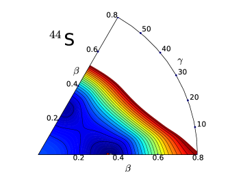
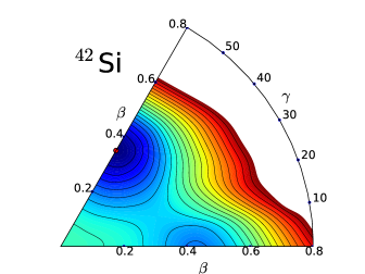
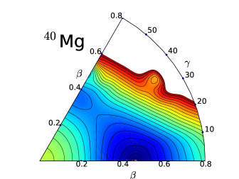
Figure 1: Self-consistent triaxial quadrupole constrained energy surfaces of $N=28$ isotones in the $\beta-\gamma$ plane ($0\leq\gamma\leq 60^{0}$). For each nucleus energies are normalized with respect to the binding energy of the global minimum. The contours join points on the surface with the same energy, and the spacing between neighbouring contours is 0.5 MeV.

Rapid transitions between equilibrium shapes in a chain of isotones (isotopes) are governed by the evolution of the shell structure of single-nucleon orbitals. In particular, one or more close-lying deformed minima can develop as a result of the occurrence of gaps or regions of low single-particle level density around the Fermi surface at finite deformation. In the present analysis we illustrate this phenomenon with the example of shape coexistence in ⁴⁴S.

There are many experimental indications for the transitional nature of ⁴⁴S: the low-lying $0_{2}^{+}$ and $2_{1}^{+}$ excited states, the large value of the reduced transition probability $B(E2,2_{1}^{+}\to 0_{1}^{+})$ [29, 30], the monopole strength $\rho^{2}(E0,0_{2}^{+}\to 0_{1}^{+})$, and the reduced transition probability $B(E2,2_{1}^{+}\to 0_{2}^{+})$ determined in a recent experiment [31]. Based on these results, shell model calculations and a simple two-level mixing model have shown that ⁴⁴S exhibits a shape coexistence between a prolate ground state and a spherical $0_{2}^{+}$ excited state. On the other hand, spectroscopic calculations based on the self-consistent mean-field approach indicate a coexistence of prolate and oblate shapes in ⁴⁴S [28, 27]. In a very recent shell model study several inconsistencies in previous interpretations of data for ⁴⁴S have been resolved [32]. Using quadrupole invariants to determine axial and triaxial shape parameters from a shell model calculation, a pronounced triaxial shape for the ground state and a slightly more pronounced prolate shape for the excited $0_{2}^{+}$ state have been predicted. It has been shown that these states display a large overlap in the $(\beta,\gamma)$ plane. Higher-lying members of the ground-state band show a tendency towards prolate deformation, whereas strong fluctuations have been predicted in the band built on top of the state $0_{2}^{+}$. An isomeric state $4_{1}^{+}$ was recently observed in ⁴⁴S [33], and the nature of this state has been explored in a shell model study [34] which has shown that this state most probably corresponds to a two-quasiparticle $K=4$ configuration.

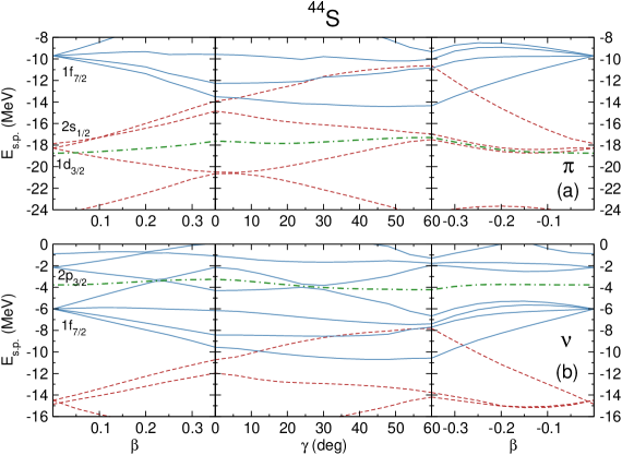
Figure 2: Proton (upper panel) and neutron (lower panel) single-nucleon energy levels of ⁴⁴S, as functions of the deformation parameters along a closed path in the $\beta-\gamma$ plane. Solid (blue) curves correspond to levels with negative parity, and (red) dashed curves denote positive-parity levels. The dot-dashed (green) curves corresponds to the Fermi levels. The panels on the left and right display prolate ($\gamma=0^{\circ}$) and oblate ($\gamma=60^{\circ}$) axially-symmetric single-particle levels, respectively. In the middle panel the proton and neutron levels are plotted as functions of $\gamma$ for a fixed value $|\beta|=0.35$.

In Fig. 2 we plot the proton (upper panel) and neutron (lower panel) single-particle levels in the canonical basis for ⁴⁴S. Solid (blue) curves correspond to levels with negative parity, and dashed (red) curves denote positive-parity levels. The dot-dashed (green) curves correspond to the Fermi levels. The proton and neutron levels are plotted as functions of the deformation parameters along a closed path in the $\beta$-$\gamma$ plane. The panels on the left and right display prolate ($\gamma=0^{\circ}$) and oblate ($\gamma=60^{\circ}$) axially symmetric single-particle levels, respectively. In the middle panel of each figure the neutron and proton levels are plotted as functions of $\gamma$ for a fixed value of the axial deformation $|\beta|=0.35$ which corresponds to the position of the prolate mean-field minimum in ⁴⁴S isotope (cf. Fig. 1). Starting from the spherical configuration, we follow the single-nucleon levels on a path along the prolate axis up to the approximate position of the minimum (left panel), then for this fixed value of $\beta$ the path from $\gamma=0^{\circ}$ to $\gamma=60^{\circ}$ (middle panel) and, finally, back to the spherical configuration along the oblate axis (right panel). Axial deformations with $\gamma=60^{\circ}$ are denoted by negative values of $\beta$. This figure illustrates the principal characteristics of structural changes in neutron-rich $N=28$ nuclei: the near degeneracy of the $d_{3/2}$ and $s_{1/2}$ proton orbitals, and the reduction of the size of the $N=28$ shell gap [35]. Between the doubly magic ⁴⁸Ca and ⁴⁴S the spherical gap $N=28$ decreases from 4.73 MeV to 3.86 MeV, respectively. Consequently, the largest gap between neutron states at the Fermi surface is located on the oblate axis (lower panel of Fig. 2), and we also notice the increased density of single-neutrons levels close to the Fermi surface at $\gamma\approx 30^{\circ}$ which leads to formation of the potential barrier in the triaxial region. For the protons (upper panel of Fig. 2), the largest gap is located on the prolate axis. The competition between pronounced proton-prolate and neutron-oblate energy gaps is at the origin of the coexistence of deformed shapes in ⁴⁴S.

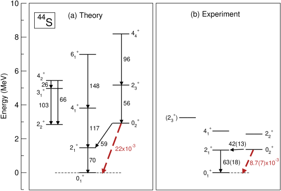
Figure 3: The theoretical excitation spectrum of ⁴⁴S (left), compared to data [30, 31, 33] (right). The $B(E2)$ values are in units of $e^{2}$fm⁴. The comparison of the monopole transition strength $\rho^{2}(E0;0_{2}^{+}\to 0_{1}^{+})$ with the experimental value is also included.

Starting from constrained self-consistent solutions of the relativistic Hartree-Bogoliubov (RHB) equations at each point on the energy surfaces (Fig. 1), we calculate the mass parameters $B_{\beta\beta}$, $B_{\beta\gamma}$, $B_{\gamma\gamma}$, the three moments of inertia $\mathcal{I}_{k}$, as well as the zero-point energy corrections, that determine the collective Hamiltonian (5). The diagonalization of the resulting Hamiltonian yields the excitation energies and reduced transition probabilities. Physical observables are calculated in the full configuration space and there are no effective charges in the model. In Fig. 3 we display the low-energy spectrum of ⁴⁴S in comparison to available data for the excitation energies, reduced electric quadrupole transition probabilities $B(E2)$ (in units of $e^{2}$fm⁴), and the electric monopole transition strength $\rho^{2}(E0;0_{2}^{+}\to 0_{1}^{+})$. The model reproduces both the excitation energy and the reduced transition probability $B(E2;2_{1}^{+}\to 0_{1}^{+})$ for the first excited state $2_{1}^{+}$. The theoretical value for $B(E2;0_{2}^{+}\to 2_{1}^{+})$ is also in good agreement with the data. However, the calculated excitation energy of the $0_{2}^{+}$ state is much higher than the experimental counterpart, and the monopole transition strength $\rho^{2}(E0;0_{2}^{+}\to 0_{1}^{+})$ overestimates the experimental value considerably. This indicates that there is probably more mixing between the theoretical states $0_{1}^{+}$ and $0_{2}^{+}$ than what can be inferred from the data. We also note that very recently the low-lying state $4_{1}^{+}$ has been interpreted as a $K=4$ isomer dominated by the two-quasiparticle configuration $\nu\Omega^{\pi}=1/2^{-}\otimes\nu\Omega^{\pi}=7/2^{-}$ [34], a configuration not included in our collective model space.

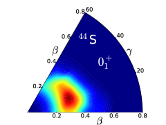
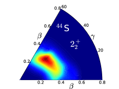
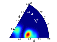
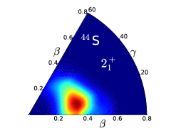
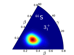
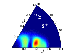
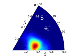
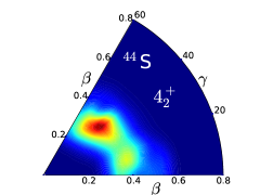
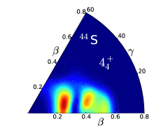
Figure 4: Probability distributions Eq. (11) in the $\beta-\gamma$ plane for the lowest collective states of ⁴⁴S.

To illustrate the degree of configuration mixing and shape coexistence in ⁴⁴S, in Fig. 4 we plot the probability density distributions for the lowest three states in the ground-state band (left), the (quasi) $\gamma$-band (middle), and the excited band built on the state $0_{2}^{+}$ (right). For a given collective state, the probability distribution in the $(\beta,\gamma)$ plane is defined as

$$\rho_{I\alpha}(\beta,\gamma)=\sum_{K\in\Delta I}{\left|\psi_{\alpha K}^{I}(\beta,\gamma)\right|^{2}\beta^{3}},$$ (11)

with the summation over the allowed set of values of the projection $K$ of the angular momentum $I$ on the body-fixed symmetry axis, and with the normalization

$$\int_{0}^{\infty}{\beta d\beta\int_{0}^{2\pi}{\rho_{I\alpha}(\beta,\gamma)|\sin{3\gamma}|d\gamma}}=1.$$ (12)

Table 1: Percentage of the $K=0$ and $K=2$ components (projection of the angular momentum on the body-fixed symmetry axis) for the collective wave functions of the three lowest $2^{+}$ states in ⁴⁴S, and the corresponding spectroscopic quadrupole moments (in $e$fm²).

	$K=0$	$K=2$	$Q_{spec}$
$2_{1}^{+}$	$89\%$	$11\%$	$-10.8$
$2_{2}^{+}$	$21\%$	$79\%$	$8.2$
$2_{3}^{+}$	$78\%$	$22\%$	$-7.3$

The probability distribution of the ground state $0_{1}^{+}$ displays a deformation $|\beta|\geq 0.3$, extended in the $\gamma$ direction from the prolate $\gamma=0^{\circ}$ to the oblate $\gamma=60^{\circ}$ shape. The $\gamma$ softness of the $0_{1}^{+}$ state reflects the ground-state mixing of configurations based on the prolate and oblate minima of the mean-field potential (cf. Fig. 1). States of the ground-state band with higher angular momenta are progressively concentrated on the prolate axis and the average $\beta$ deformation gradually increases because of centrifugal stretching. Although the $0_{2}^{+}$ state is predominantly prolate, one notices oblate admixtures and, consequently, a relatively large overlap between the wave functions of $0_{1}^{+}$ and $0_{2}^{+}$. The mixing between these states leads to a pronounced level repulsion which is probably the cause for the too high excitation energy of the theoretical state $0_{2}^{+}$. The low-lying $0_{2}^{+}$ state at $1.365$ MeV and the monopole strength $\rho^{2}(E0;0_{2}^{+}\to 0_{1}^{+})=8.7(7)\times 10^{-3}$ have been regarded as signatures of prolate-spherical shape coexistence in ⁴⁴S [31]. However, recent studies have re-examined the structure of ⁴⁴S [32], emphasizing the effect of the triaxial degree of freedom on the low-lying excitation structure. The probability distribution of $2_{3}^{+}$ is concentrated on the prolate axis and the transition strength $B(E2;2_{3}^{+}\to 0_{2}^{+})$ is comparable to $B(E2;2_{1}^{+}\to 0_{1}^{+})$. For the three lowest $2^{+}$ levels, in Table 1 we list the percentage of the $K=0$ and $K=2$ components in the collective wave functions, together with the spectroscopic quadrupole moments. The wave functions of the states $2_{1}^{+}$ and $2_{3}^{+}$ are dominated by the $K=0$ components, and the spectroscopic quadrupole moments indicate prolate configurations. In contrast the positive quadrupole moment of $2_{2}^{+}$ state points to a predominantly oblate configuration, while the $\approx 80\%$ contribution of the $K=2$ component in the wave function shows that this state is the band-head of a (quasi) $\gamma$-band. One also notices the close-lying doublet $3_{1}^{+}$ and the $4_{2}^{+}$, characteristic for a $K=2$ band in a $\gamma$-soft potential.

The example considered in this section and similar calculations reported recently have shown that the EDF approach provides an accurate microscopic interpretation of the reduction of the $N=28$ spherical energy gap in neutron-rich nuclei, and a quantitative description of the evolution of shapes in $N=28$ isotones in terms of single-nucleon orbitals as functions of the quadrupole deformation parameters $\beta$ and $\gamma$. In particular, the formation of the oblate neutron and prolate proton gaps in ⁴⁴S, illustrated in Fig. 2, is at the origin of the predicted shape coexistence, in very good agreement with recent data.

4 Lowest $\bm{0^{+}}$ excitations in $\bm{N\approx 90}$ rare-earth nuclei

Rare-earth nuclei with neutron number $N\approx 90$ present some of the best examples of rapid shape evolution and shape phase transitions [1, 4, 36]. Employing a consistent framework of structure models (GCM, quadrupole collective Hamiltonian) based on relativistic energy density functionals, in a series of studies [37, 38, 39] we analysed microscopic signatures of ground-state shape phase transitions in this region of the nuclear mass table. Phase transitions in equilibrium shapes of atomic nuclei correspond to first- and second-order quantum phase transitions (QPT) between competing ground-state phases induced by variation of a non-thermal control parameter (number of nucleons) at zero temperature. In general, one observes a a gradual evolution of shapes with the number of nucleons, and these transitions reflect the underlying modifications of shell structure and interactions between valence nucleons. A phase transition, on the other hand, is characterised by a significant variation of one or more order parameters as functions of the control parameter. Even though in systems composed of a finite number of particles phase transitions are actually smoothed out, in many cases clear signatures of abrupt changes of structure properties are observed. A number of experiments over the last two decades, as well as many theoretical studies of deformation energy surfaces and also direct computation of observables related to order parameters, have shown that two-neutron separation energies, isotope shifts, energy gaps between the ground state and the excited vibrational states with zero angular momentum, isomer shifts, and monopole transition strengths, exhibit sharp discontinuities at neutron number $N=90$.

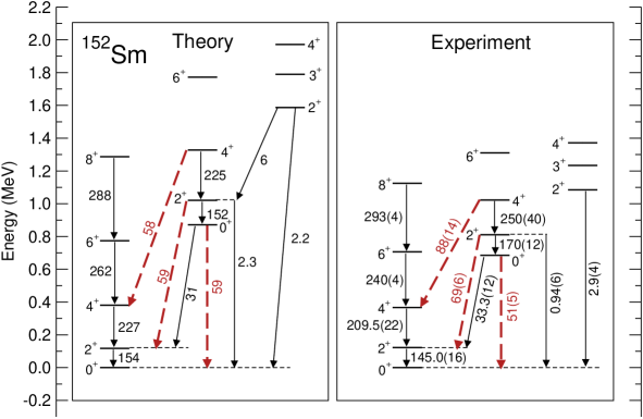
Figure 5: The theoretical excitation spectrum of ¹⁵²Sm (left), compared to data [40]. The intraband and interband B(E2) values (thin solid arrows) are in Weisskopf units(W.u.), and (red) dashed arrows denote E0 transitions with the corresponding $\rho^{2}(E0)\times 10^{3}$ values.

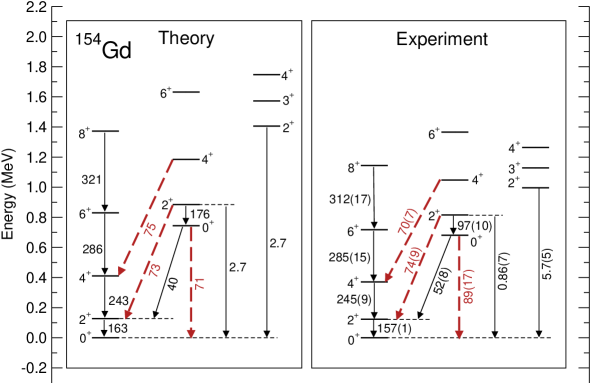
Figure 6: Same as in the caption to Fig. 5 but for ¹⁵⁴Gd.

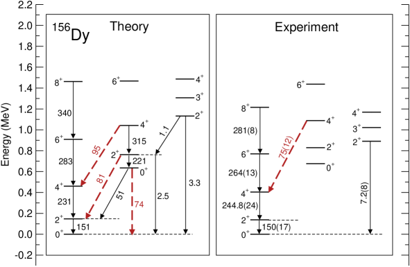
Figure 7: Same as in the caption to Fig. 5 but for ¹⁵⁶Dy.

In the present study we focus on the low-lying $0^{+}$ excitations in the deformed $N=90$ isotones and examine the mixing between the lowest $K=0$ bands. Traditionally the first excited $0^{+}$ level in deformed nuclei has been interpreted as a $\beta$-vibrational state, with the associated $K=0$ rotational $\beta$-band. However, many experimental studies have shown that most of the $0^{+}_{2}$ excitations are not $\beta$ vibrations. In the exhaustive review of properties of the lowest-lying $0^{+}$ states in deformed rare-earth nuclei [41], it was emphasized that there is no a priori reason to associate the $\beta$ vibration with the lowest $0^{+}$ excited state. A set of properties was suggested that the first excited $0^{+}$ level should exhibit in order to be labelled as a $\beta$ vibration. Among those: $B(E2;0^{+}_{\beta}\to 2^{+}_{1})$ values of $12-33$ W.u. or conversely $B(E2;2^{+}_{\beta}\to 0^{+}_{1})$ of $2.5-6$ W.u., and $\rho^{2}(E0;{0^{+}_{2}\to 0^{+}_{1}})\times 10^{3}$ values of $85-230$. In our microscopic analysis of order parameters in nuclear quantum phase transitions [39], in particular for the Nd isotopic chain, it was shown that the excitation energies of both $0^{+}_{2}$ and $0^{+}_{3}$ exhibit a pronounced dip at $N=90$, which can be attributed to the softness of the potential with respect to $\beta$ deformation in ¹⁵⁰Nd. The calculated monopole transition strengths exhibit a pronounced increase toward $N=90$, and the $\rho^{2}(E0;{0^{+}_{2}\to 0^{+}_{1}})$ values remain rather large in the deformed nuclei ^152,154,156Nd, a behaviour characteristic for an order parameter at the point of first-order QPT.

In Figs. 5 - 7 we plot the theoretical low-energy spectra of the $N=90$ nuclei: ¹⁵²Sm, ¹⁵⁴Gd and ¹⁵⁶Dy, in comparison with data [40]. The ground-state bands, lowest $K=0$ and $K=2$ bands are compared to their experimental counterparts: excitation energies, intraband and interband $B(E2)$ values, and $E0$ transition strengths. The theoretical spectra comprise eigenstates of the five-dimensional quadrupole collective Hamiltonian (5), based on triaxial SCMF solutions obtained with the density functional DD-PC1 and a finite-range pairing force separable in momentum space. No additional parameters are adjusted to data, and transition rates have been calculated with bare charges, that is, $e_{p}=e$ and $e_{n}=0$.

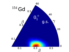
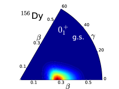
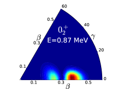
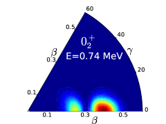
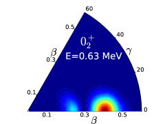
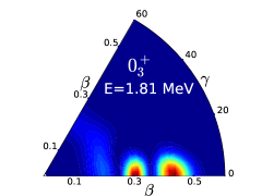
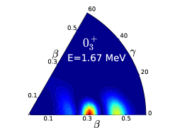
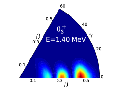
Figure 8: Probability distributions Eq. (11) in the $\beta-\gamma$ plane for the lowest collective $0^{+}$ states of ¹⁵²Sm, ¹⁵⁴Gd and ¹⁵⁶Dy.

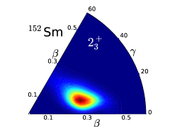
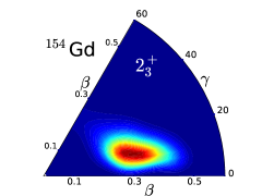
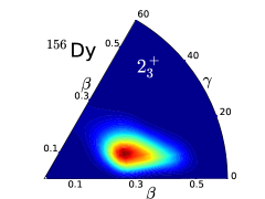
Figure 9: Probability distributions Eq. (11) in the $\beta-\gamma$ plane for the band-heads of the $K=2$ $\gamma$-bands of ¹⁵²Sm, ¹⁵⁴Gd and ¹⁵⁶Dy.

For the ground-state bands the theoretical excitation energies and $B(E2)$ values for transitions within the band are in very good agreement with data, except for the fact that the empirical moments of inertia are systematically larger than those calculated with the collective Hamiltonian. This is a well known effect of using the simple Inglis-Belyaev approximation for the moments of inertia, and is also reflected in the excitation energies of the excited $K=0$ and $K=2$ bands [42]. The wave functions, however, are not affected by this approximation and we note that the model reproduces both the intraband and interband $E2$ transition probabilities. The $K=2$ $\gamma$-bands are predicted at somewhat higher excitation energies compared to their experimental counterparts, and this is most probably due to the potential energy surfaces being too stiff in $\gamma$. The deformed rare-earth $N=90$ isotones are characterised by very low $K=0$ bands based on the $0^{+}_{2}$ states. In ¹⁵²Sm, for instance, this state is found at 685 keV excitation energy, considerably below the $K=2$ $\gamma$-band. Nevertheless, this state has been interpreted as the band-head of the $\beta$-band [41, 42].

In ¹⁵²Sm the excited $K=0$ band is calculated at moderately higher energy compared to data, while the agreement with experiment is very good for ¹⁵⁴Gd and ¹⁵⁶Dy. We note that a very similar excitation spectrum for ¹⁵²Sm was also obtained with the collective Hamitonian based on the D1S Gogny interaction [42]. Particularly important for the present study are the $E0$ transitions between the two lowest $K=0$ bands, and the $B(E2;0^{+}_{2}\to 2^{+}_{1})$ and $B(E2;2^{+}_{2}\to 0^{+}_{1})$ values. The available data are very accurately reproduced by the calculation and, in particular for ¹⁵²Sm, the $E0$ transition strengths and $B(E2)$ values seem to match the criteria for a $\beta$-vibrational state [41].

The $E0$ transitions strengths reflect the degree of mixing between the two lowest $K=0$ bands, and Figs. 5 - 7 show that the theoretical values that correspond to transitions between the eigenstates of the collective Hamiltonian reproduce the empirical $\rho^{2}(E0)$ values. The structure of the low-lying $0^{+}$ states is analysed in Fig. 8, in which the probability density distributions are plotted in the $\beta-\gamma$ plane for the three lowest collective $0^{+}$ states of ¹⁵²Sm, ¹⁵⁴Gd and ¹⁵⁶Dy. We note that the probability distributions for these states are concentrated on the prolate axis $\gamma=0^{\circ}$, in contrast to the band-heads of the $K=2$ $\gamma$-bands, for which the probability density distributions are shown in Fig. 9. The dynamical $\gamma$-deformations of the latter clearly point to the $\gamma$-vibrational nature of these states. The average values of the deformation parameter $\beta$ for the collective ground-state wave functions of ¹⁵²Sm: $<\beta>=0.32$, ¹⁵⁴Gd: $<\beta>=0.31$, and ¹⁵⁶Dy: $<\beta>=0.30$, correspond to the minimum of the respective deformation energy surface. The corresponding values for the first excited $0^{+}$ states are: $<\beta>=0.33$ for ¹⁵²Sm, $<\beta>=0.34$ for ¹⁵⁴Gd, and $<\beta>=0.37$ for ¹⁵⁶Dy. For a pure harmonic $\beta$-vibrational state one expects that the average deformation is the same as for the ground-state, that the ratio of $\Delta\beta$ values for $0^{+}_{\beta}$ with respect to $0^{+}_{1}$ is $\sqrt{3}$, and that the probability density distribution displays one node at $<\beta>_{\rm g.s.}$ and two peaks of the same amplitude. The ratio of $\Delta\beta$ values for $0^{+}_{2}$ with respect to $0^{+}_{1}$ is: 1.6 for ¹⁵²Sm, 1.53 for ¹⁵⁴Gd, and 1.42 for ¹⁵⁶Dy. Considering all these quantities, it appears that the best candidate for the $\beta$-vibrational state is $0^{+}_{2}$ in ¹⁵²Sm. However, even in this case the probability distribution does not display two peaks of equal amplitude, and the shift to larger deformation is more pronounced in ¹⁵⁴Gd and ¹⁵⁶Dy. Note that for the latter two nuclei the calculated excitation energy of the $0^{+}_{2}$ states are in even better agreement with data. The probability distributions for the $0^{+}_{3}$ levels, plotted in the third row of Fig. 8, indicate the development of a second node and third peak, that is, the appearance of two-phonon states. One notices, however, the mixing with states based on $\gamma$ vibrations, which becomes even more pronounced for higher lying $0^{+}$ states, not shown in the figure. An experimental exploration of a possible occurrence of multiple (two) phonon intrinsic collective excitations in ¹⁵²Sm did not find evidence for two-phonon $K^{\pi}=0^{+}$ quadrupole vibrations [43]. In fact, it has been argued that an emerging pattern of repeating excitations built on $0^{+}_{2}$, similar to those based on the ground state, shows that ¹⁵²Sm is an example of shape coexistence [44].

The simple analysis presented in this section illustrates the complex structure of excited $0^{+}$ levels in deformed nuclei, and the difficulties in classifying these states as simple collective vibrational states, that is, as one and two-phonon $\beta$ vibrations. A more quantitative theoretical investigation should involve additional effects not included in our collective Hamiltonian model, such as are the coupling between shape oscillations and pairing vibrations [45] and, in general, the coupling between collective and intrinsic two-quasiparticle excitations [46], that can lower the collective energy levels and improve the agreement with data [40, 41]. In particular, a more advanced model that includes coupling between collective and intrinsic two-quasiparticle excitations can be used to analyse excited rotational bands based on pairing isomers, such as those identified in ¹⁵⁴Gd [47] and ¹⁵²Sm [48].

5 Quadrupole and octupole shape transition in Thorium

Most deformed medium-heavy and heavy nuclei display quadrupole equilibrium shapes, but there are also regions of the mass table in which octupole deformations (reflection-asymmetric, pear-like shapes) occur. Reflection-asymmetric shapes are characterized by the presence of negative-parity bands, and by pronounced electric dipole and octupole transitions. In the case of static octupole deformations, for instance, the lowest positive-parity even-spin states and the negative-parity odd-spin states form an alternating-parity band, with states connected by the enhanced E1 transitions. In a simple microscopic picture strong octupole correlations arise through a coupling of orbitals near the Fermi surface with quantum numbers ($l$, $j$) and ($l+3$, $j+3$). This leads to reflection-asymmetric intrinsic shapes that develop either dynamically (octupole vibrations) or as static octupole equilibrium deformations [2, 49]. For example, in the case of $N\approx 134$ and $Z\approx 88$ nuclei in the region of light actinides, the coupling of the neutron orbitals based on $g_{9/2}$ and $j_{15/2}$, and that of the proton single-particle states arising from $f_{7/2}$ and $i_{13/2}$, can give rise to octupole mean-field deformations.

An interesting phenomenon are simultaneous quadrupole and octupole shape transitions. In a series of recent studies [50, 51, 52] we have analyzed the evolution of quadrupole and octupole shapes using a consistent microscopic framework based on relativistic EDFs. In thorium isotopes, in particular, the calculated triaxial quadrupole and axial quadrupole-octupole energy surfaces, and predicted observables (excitation energies, isotope shifts of charge radii, electromagnetic transition rates) point to the occurrence of a simultaneous phase transition between spherical and quadrupole-deformed prolate shapes, and between non-octupole and octupole-deformed shapes, with ²²⁴Th being closest to the critical point of the double shape phase transition [51].

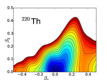
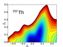
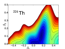
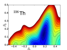
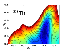
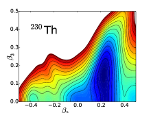
Figure 10: Axially symmetric energy surfaces of the isotopes ^220-230Th in the $(\beta_{2},\beta_{3})$ plane. The contours join points on the surface with the same energy and the energy difference between neighboring contours is 1 MeV. Positive (negative) values of $\beta_{2}$ correspond to prolate (oblate) configurations. Energy surfaces are symmetric with respect to the $\beta_{3}=0$ axis.

Figure 10 displays the deformation energy surfaces in the plane of axial quadrupole and octupole deformation parameters ($\beta_{2}$, $\beta_{3}$) for the isotopes ^220-230Th. This isotopic chain exhibits an interesting structural evolution, visible already at the SCMF level. A rather soft energy surface is calculated for ²²⁰Th with the minimum at $(\beta_{2},\beta_{3})\approx(0,0)$, and this will give rise to quadrupole vibrational excitation spectra. Quadrupole deformation becomes more pronounced in ²²⁴Th, and one also notices the emergence of octupole deformation. The energy minimum is found in the $\beta_{3}\neq 0$ region, located at $(\beta_{2},\beta_{3})\approx(0.1,0.1)$ . From ²²⁴Th to ²²⁸Th the occurrence of a rather strongly marked octupole minimum is predicted. Starting from ²²⁸Th, the minimum becomes softer in the octupole $\beta_{3}$ direction. An octupole-soft surface, almost completely flat in $\beta_{3}$ for $\beta_{3}\leq 0.3$, is calculated for ²³²Th.

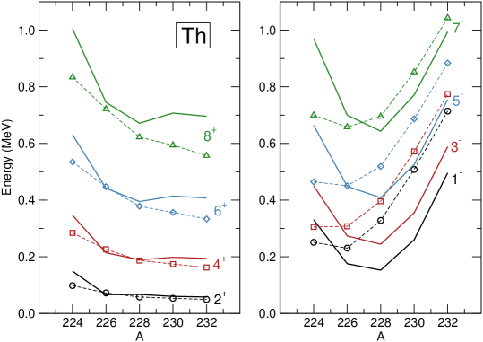
Figure 11: Excitation energies of low-lying yrast positive-parity (left) and negative-parity (right) collective states of ^224-232Th. Lines and symbols denote the theoretical and experimental [40] levels, respectively.

In Fig. 11 we analyse the systematics of energy spectra of the positive-parity ground-state band ($K^{\pi}=0^{+}$) (left) and the lowest negative-parity ($K^{\pi}=0^{-}$) sequences (right) in ^224-232Th. The theoretical values calculated using the quadrupole-octupole collective Hamiltonian (9) are shown in comparison to available data [40]. The excitation energies of positive-parity states systematically decrease with mass number, reflecting the increase of quadrupole collectivity. ^220,222Th exhibit a quadrupole vibrational structure, whereas pronounced ground-state rotational bands with $R_{4/2}=E(4^{+}_{1})/E(2^{+}_{1})\approx 3.33$ are calculated in ^226-232Th. For the lowest negative-parity bands the excitation energies display a parabolic structure centered between ²²⁴Th and ²²⁶Th. The approximate parabola of $1^{-}_{1}$ states has a minimum at ²²⁶Th, in which the octupole deformed minimum is most pronounced. Starting from ²²⁶Th the energies of negative-parity states systematically increase and the band becomes more compressed. A rotational-like collective band based on the octupole vibrational state, i.e., the $1^{-}_{1}$ band-head, develops. The parabolas of negative-parity states calculated with the quadrupole-octupole Hamiltonian are in qualitative agreement with data, although the minima are predicted to occur at ²²⁸Th rather than ²²⁶Th. Note, however, that all levels shown in Fig. 11 are below 1 MeV excitation energy, so that the differences between calculated and experimental levels are rather small, especially considering that no parameters were adjusted to data. The approximations involved in the calculation of the Hamiltonian parameters (perturbative cranking for the mass parameters and the Inglis-Belyaev formula for the moments of inertia) determine the level of quantitative agreement with experiment. We note that the theoretical B(E2) values for transitions within the ground state bands are in agreement with availabe data, while the calculated $B(E3;3^{-}_{1}\to 0^{+}_{1})$: 61 W.u. for ²³⁰Th and 41 W.u. for ²³²Th, are somewhat larger than the experimental values: 29(3) W.u. for ²³⁰Th and 24(3) W.u. for ²³²Th [53].

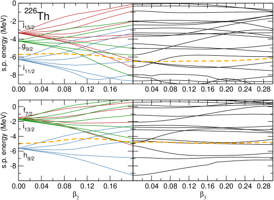
Figure 12: ²²⁶Th single-neutron (upper panel) and single-proton (lower panel) levels in the canonical basis as functions of the deformation parameters. The path follows the quadrupole deformation parameter $\beta_{2}$ up to the position of the equilibrium minimum $\beta_{2}=0.2$, with the constant octupole deformation $\beta_{3}=0$ (left panels). For $\beta_{2}=0.2$ the panels on the right display the single-nucleon energies from $\beta_{3}=0$ to $\beta_{3}=0.3$. Dashed curves denote the position of the Fermi level at each deformation.

Let us consider in more detail the structure of ²²⁶Th which, at the SCMF level, exhibits a nice example of coexistence of axial quadrupole and octupole minima. The energy difference between the local minimum at $\beta_{3}=0$ and the equlibrium minimum at $\beta_{3}=0.16$ is 1.8 MeV. We have also carried out a constrained triaxial quadrupole SCMF calculation which confirms that the quadrupole minimum is indeed at $\gamma=0^{\circ}$, that is, axial prolate. The microscopic origin of coexistence of the two minima becomes apparent from the dependence of the single-nucleon levels on the two deformation parameters. Figure 12 displays the single neutron and proton levels of ²²⁶Th along a path in the $\beta_{2}-\beta_{3}$ plane. Starting from the spherical configuration, the path follows the quadrupole deformation parameter $\beta_{2}$ up to the position of the equilibrium minimum $\beta_{2}=0.2$, with the octupole deformation parameter kept constant at zero value. Then, for the constant value $\beta_{2}=0.2$, the path continues from $\beta_{3}=0$ to $\beta_{3}=0.3$. The necessary condition for the occurrence of low-energy octupole collectivity is the presence of pairs of orbitals near the Fermi level that are strongly coupled by the octupole interaction. In the panels on the left of Fig. 12 we notice states of opposite parity that originate from the spherical levels $g_{9/2}$ and $j_{15/2}$ for neutrons, and $f_{7/2}$ and $i_{13/2}$ for protons. The total energy can be related to the level density around the Fermi surface, that is, a lower-than-average density of single-particle levels results in extra binding. Therefore, the local quadrupole minimum seen on the axial energy surface of ²²⁶Th reflects the $\beta_{2}$-dependence of the levels of the Nilsson diagram for $\beta_{3}=0$. For the levels in the panels on the right of Fig. 12 parity is not conserved, and the only quantum number that characterises these states is the projection of the angular momentum on the symmetry axis. The octupole minimum, rather soft along the $\beta_{3}$-path in ²²⁶Th, is attributed to the low density of both proton and neutron states close to the corresponding Fermi levels in the interval of deformations around $\beta_{3}=0.16$.

Fully microscopic analyses of coexistence of quadrupole and octupole shapes and, in general, the evolution of octupole correlations in heavy nuclei, will be particularly important for future experimental studies of reflection-asymmetric shapes using accelerated radioactive beams [54], and in searches for new symmetry violating interactions beyond the standard model [49].

6 Summary

The framework of nuclear energy density functionals provides an intuitive and yet accurate microscopic interpretation of the evolution of single-nucleon shell structure and the related phenomena of deformations, shape transitions and shape coexistence. Self-consistent mean-field calculations of deformation energy surfaces produce symmetry-breaking many-body states that include important static correlations such as deformations and pairing. Intrinsic shapes that correspond to minima on the deformation energy surface are determined by the static (constrained) collective coordinates. Dynamical correlations are included by collective structure models that restore symmetries broken by the static mean field and take into account quantum fluctuations of collective variables. The microscopic input for the generator coordinate method or the collective Hamiltonian model are completely determined by the choice of the energy density functional and pairing interaction. These models can be used to calculate observables that characterise the evolution and eventual coexistence of different shapes: low-energy excitation spectra, electromagnetic transition rates, changes in masses (separation energies), isotope and isomer shifts, and that can be directly compared to data.

Using a single relativistic energy density functional and a finite-range pairing interaction separable in momentum space, in the present study we have analysed illustrative examples of diverse phenomena related to evolution of shell structure: shape transition and coexistence in neutron-rich $N=28$ isotones, the structure of lowest $0^{+}$ excitations in deformed $N=90$ rare-earth nuclei, and quadrupole and octupole shape transitions in thorium isotopes. Spectroscopic properties have been calculated using the five-dimensional quadrupole and axial quadrupole-octupole collective Hamiltonian models. The very good agreement between theoretical predictions and available data, and especially the fact that very different regions of the mass table could be considered with no need to adjust or fine-tune model parameters to specific data, demonstrate that the approach based on universal density functionals is a method of choice for studies of shape transitions and coexistence over the entire table of nuclides, including regions of exotic short-lived nuclei far from stability.

Future developments of structure methods based on nuclear energy density functionals include a number of major challenges. One of the most important and certainly most difficult is the construction of a consistent set of approximations for the exchange-correlation energy functional. In the context of phenomena discussed in the present analysis, it would be very interesting to try to develop microscopic functionals that, in addition to the dependence on ground-state densities and currents composed of occupied Kohn-Sham orbitals, also include a dependence on unoccupied orbitals. This is particularly important for studies of the evolution of shell structure and modification of gaps in nuclei far from stability and/or superheavy nuclei. For quantitative comparison with available spectroscopic data and predictions in new regions of the chart of nuclides, accurate and efficient algorithms have to be developed that perform a complete restoration of symmetries broken by self-consistent mean-field solutions for general quadrupole and octupole shapes. Deformation-dependent parameters of collective quadrupole (-octupole) Hamiltonians (vibrational inertial functions and moments of inertia) need to be determined using methods that go beyond the simple cranking formulas and include the full dynamics of a nuclear system. Finally, theoretical studies of low-energy spectroscopic properties that characterise shape coexistence will also have to include uncertainty estimates, quantify theoretical errors and evaluate correlations between observables.

References

- [1] K. Heyde and J. L. Wood, Rev. Mod. Phys. 83, 1467 (2011).
- [2] P. A. Butler and W. Nazarewicz, Rev. Mod. Phys. 68, 349 (1996)
- [3] O. Sorlin and M.-G. Porquet, Prog. Part. Nucl. Phys. 61, 602 (2008).
- [4] P. Cejnar, J. Jolie, and R. F. Casten, Rev. Mod. Phys. 82, 2155 (2010).
- [5] M. Bender, P.-H. Heenen, and P.-G. Reinhard, Rev. Mod. Phys. 75, 121 (2003).
- [6] D. Vretenar, A.V. Afanasjev, G.A. Lalazissis, and P. Ring, Phys. Rep. 409, 101 (2005).
- [7] G. A. Lalazissis, P. Ring, and D. Vretenar (Eds.), Extended Density Functionals in Nuclear Structure Physics, Lecture Notes in Physics 641, (Springer, Heidelberg 2004.)
- [8] J. R. Stone and P.-G. Reinhard, Prog. Part. Nucl. Phys. 58, 587 (2007).
- [9] R. B. Laughlin, D. Pines, J. Schmalian, B. P. Stojković, and P. Wolynes, Proc. Natl. Acad. Sci. 97, 32 (2000).
- [10] T. Nikšić, D. Vretenar, and P. Ring, Prog. Part. Nucl. Phys. 66, 519 (2011).
- [11] T. Duguet, Lecture Notes in Physics 879, (Springer, Heidelberg 2014) p. 293
- [12] P. Ring and P. Schuck, The Nuclear Many-Body Problem (Springer-Verlag, Heidelberg, 1980).
- [13] M. Bender and P.-H. Heenen, Phys. Rev. C 78, 024309 (2008).
- [14] T. R. Rodríguez and J. L. Egido, Phys. Rev. C 81, 064323 (2010).
- [15] J. M. Yao, J. Meng, P. Ring, and D. Vretenar, Phys. Rev. C 81, 044311 (2010).
- [16] B. Bally, B. Avez, M. Bender, and P.-H. Heenen, Phys. Rev. Lett. 113, 162501 (2014).
- [17] P.-G. Reinhard and K. Goeke, Rep. Prog. Phys. 50, 1 (1987).
- [18] L. Próchniak and S. G. Rohoziński, J. Phys. G 36, 123101 (2009).
- [19] K. Goeke and P.-G. Reinhard, Ann. Phys. (N.Y.) 124, 249 (1980).
- [20] J. -P. Delaroche, M. Girod, J. Libert, H. Goutte, S. Hilaire, S. Péru, N. Pillet, and G. F. Bertsch, Phys. Rev. C 81, 014303 (2010).
- [21] T. Nikšić, D. Vretenar, P. Ring, Phys. Rev. C 78, 034318 (2008).
- [22] Y. Tian, Z. Y. Ma, P. Ring, Phys. Lett. B 676, 44 (2009).
- [23] J. M. Yao, K. Hagino, Z. P. Li, J. Meng, and P. Ring Phys. Rev. C 89, 054306 (2014).
- [24] T. Nikšić, Z. P. Li, D. Vretenar, L. Próchniak, J. Meng, and P. Ring, Phys. Rev. C 79, 034303 (2009).
- [25] N. Hinohara, Z. P. Li, T. Nakatsukasa, T. Nikšić, and D. Vretenar Phys. Rev. C 85, 024323 (2012).
- [26] M. Girod and B. Grammaticos, Nucl. Phys. A 330, 40 (1979).
- [27] Z. P. Li, J. M. Yao, D. Vretenar, T. Nikšić, H. Chen, and J. Meng, Phys. Rev. C 84, 054304 (2011).
- [28] T. R. Rodríguez, J. L. Egido, Phys. Rev. C 84, 051307 (R) (2011).
- [29] S. Grévy et al., Eur. Phys. J. A 25, 111 (2005).
- [30] T. Glasmacher et al., Phys. Lett. B 395, 163 (1997).
- [31] C. Force et al., Phys. Rev. Lett. 105, 102501 (2011).
- [32] R. Chevrier, L. Gaudefroy, Phys. Rev. C 89, 051301(R) (2014).
- [33] D. Santiago-Gonzalez et al., Phys. Rev. C 83, 061305 (2011).
- [34] Y. Utsuno, N. Shimizu, T. Otsuka, T. Yoshida, Y. Tsunoda, Phys. Rev. Lett. 114, 032501 (2015).
- [35] O. Sorlin, Nucl. Phys. A 834, 400c (2010).
- [36] R. F. Casten and E. A. McCutchan, J. Phys. G: Nucl. Part. Phys. 34, R285 (2007).
- [37] T. Nikšić, D. Vretenar, G. A. Lalazissis, and P. Ring, Phys. Rev. Lett. 99, 092502 (2007).
- [38] Z. P. Li, T. Nikšić, D. Vretenar, J. Meng, G. A. Lalazissis, and P. Ring, Phys. Rev. C 79, 054301 (2009).
- [39] Z. P. Li, T. Nikšić, D. Vretenar, and J. Meng, Phys. Rev. C 80, 061301(R) (2009).
- [40] Brookhaven National Nuclear Data Center, http://www.nndc.bnl.gov.
- [41] P. E. Garrett, J. Phys. G. 27, R1 (2001).
- [42] J. -P. Delaroche, M. Girod, J. Libert, H. Goutte, S. Hilaire, S. Péru, N. Pillet, and G. F. Bertsch, Phys. Rev. C 81, 014303 (2010).
- [43] W. D. Kulp et al., Phys. Rev. C 77, 061301 (R) (2008).
- [44] P. E. Garrett et al., Phys. Rev. Lett. 103, 062501 (2009).
- [45] S. Pilat and K. Pomorski, Nucl. Phys. A 554, 413 (1993).
- [46] R. Bernard, H. Goutte, D. Gogny, and W. Younes, Phys. Rev. C 84, 044308 (2011).
- [47] W. D. Kulp et al., Phys. Rev. Lett. 91, 102501 (2003).
- [48] W. D. Kulp et al., Phys. Rev. C 71, 041303 (R) (2005).
- [49] P. A. Butler and L. Willmann, Nucl. Phys. News 25, 12 (2015).
- [50] K. Nomura, D. Vretenar, and Bing-Nan Lu, Phys. Rev. C 88, 021303(R) (2013).
- [51] Z. P. Li, B. Y. Song, J. M. Yao, D. Vretenar, and J. Meng, Phys. Lett. B 726, 866 (2013).
- [52] K. Nomura, D. Vretenar, T. Nikšić, and Bing-Nan Lu, Phys. Rev. C 89, 024312 (2014).
- [53] T. Kibedi, R.H. Spear, At. Data Nucl. Data Tables 80, 35(2002).
- [54] L. P. Gaffney et al., Nature 497, 199 (2013).