Confirming and improving post-Newtonian and effective-one-body results from self-force computations along eccentric orbits around a Schwarzschild black hole

Abstract

We analytically compute, through the six-and-a-half post-Newtonian order, the second-order-in-eccentricity piece of the Detweiler-Barack-Sago gauge-invariant redshift function for a small mass in eccentric orbit around a Schwarzschild black hole. Using the first law of mechanics for eccentric orbits [A. Le Tiec, Phys. Rev. D 92, 084021 (2015)] we transcribe our result into a correspondingly accurate knowledge of the second radial potential of the effective-one-body formalism [A. Buonanno and T. Damour, Phys. Rev. D 59, 084006 (1999)]. We compare our newly acquired analytical information to several different numerical self-force data and find good agreement, within estimated error bars. We also obtain, for the first time, independent analytical checks of the recently derived, comparable-mass fourth-post-Newtonian order dynamics [T. Damour, P. Jaranowski and G. Shaefer, Phys. Rev. D 89, 064058 (2014)].

I Introduction

Recent years have witnessed a useful synergy between various ways of tackling, in General Relativity, the two-body problem. In particular, the effective-one-body (EOB) formalism Buonanno:1998gg ; Buonanno:2000ef ; Damour:2000we ; Damour:2001tu has served as a focal point allowing one to gather and compare information contained in various other approaches to the two-body problem, such as post-Newtonian (PN) theory Schafer:2009dq ; Blanchet:2013haa , self-force (SF) theory Barack:2009ux ; Poisson:2011nh , as well as full numerical relativity simulations.

The aim of the present work is to extract new information on the dynamics of eccentric (non-spinning) binary systems from both analytical and numerical SF computations along eccentric orbits around a Schwarzcshild black hole. This new information will concern both the usual PN-expanded approach to binary systems, and its EOB formulation (which, as we shall see, is particularly useful for transforming the information between various gauge-invariant observable quantities).

The first gauge-invariant quantity we shall consider is the generalization to eccentric orbits of Detweiler’s Detweiler:2008ft inverse redshift function, namely the function

$$U\left(m_{2}\Omega_{r},m_{2}\Omega_{\phi},\frac{m_{1}}{m_{2}}\right)=\frac{\displaystyle\oint dt}{\displaystyle\oint d\tau}=\frac{T_{r}}{{\mathcal{T}}_{r}}$$ (1)

introduced by Barack and Sago Barack:2011ed .

The notation here is as follows. The two masses of the considered binary system are $m_{1}$ and $m_{2}$, with the convention $m_{1}\leq m_{2}$ (and $m_{1}\ll m_{2}$ in SF calculations). We then denote (in our EOB considerations) $M\equiv m_{1}+m_{2}$, $\mu\equiv m_{1}m_{2}/(m_{1}+m_{2})$, $\nu\equiv\mu/M=m_{1}m_{2}/(m_{1}+m_{2})^{2}$. The intensity of the gravitational potential is measured (in EOB theory) by $u=M/r$ (in the units $G=c=1$ we use). In Eq. (1) the symbol $\oint$ denotes an integral over a radial period (from periastron to periastron) so that $T_{r}=\oint dt$ denotes the coordinate-time period and ${\mathcal{T}}_{r}=\oint d\tau$ the proper-time period. In addition $\Omega_{r}=2\pi/T_{r}$ is the radial frequency and $\Omega_{\phi}=\oint d\phi/\oint dt=\Phi/T_{r}$ is the mean azimuthal frequency. The first-order SF contribution $\delta U$ to the function (1), defined by

$$U\left(m_{2}\Omega_{r},m_{2}\Omega_{\phi},\frac{m_{1}}{m_{2}}\right) = U_{0}\left(m_{2}\Omega_{r},m_{2}\Omega_{\phi}\right)$$ (2)

$$+ \frac{m_{1}}{m_{2}}\delta U\left(m_{2}\Omega_{r},m_{2}\Omega_{\phi}\right)$$

$$+ O\left(\frac{m_{1}^{2}}{m_{2}^{2}}\right)\,,$$

is conveniently represented as a function of the dimensionless semi-latus rectum $p$ and the eccentricity $e$ of the unperturbed orbit: $\delta U(p,e)$. [See below for explicit definitions.]

Our first result will be to analytically derive the eccentricity-dependent part (denoting $u_{p}\equiv 1/p$) of

$$\delta U(p,e) = \delta U^{e^{0}}(u_{p})+e^{2}\delta U^{e^{2}}(u_{p})$$ (3)

$$+ e^{4}\delta U^{e^{4}}(u_{p})+e^{6}\delta U^{e^{6}}(u_{p})+O(e^{8})$$

to order $O(u_{p}^{15/2})$ included for the $O(e^{2})$ piece $\delta U^{e^{2}}$, and to order $u_{p}^{5}$ included for the $O(e^{4})$ piece. The previous knowledge of the coefficients $\delta U^{e^{2}}$, $\delta U^{e^{4}}$, $\delta U^{e^{6}}$ was only $O(u_{p}^{4})$, corresponding to the 3PN level Tiec:2015cxa . Then we shall translate our higher-order results on $\delta U^{e^{2}}$ into a correspondingly improved result (6.5PN level) for the EOB potential $\bar{d}(u)$ entering the dynamics of eccentric orbits at the $p_{r}^{2}$ level. To do this we shall use a recent generalization to eccentric orbits, Tiec:2015cxa , of the connection between $\delta U^{e^{0}}(u_{p})$ and the $O(\nu)$ piece $a(u)$ of the main EOB radial potential Barausse:2011dq ; Akcay:2012ea . Let us note in passing that this connection has a direct link with what was, historically, the starting point of the EOB formalism, i.e., the (gauge-invariant) “action-angle” (Delaunay) form of the two-body Hamiltonian Damour:1988mr . Using the relations derived in Tiec:2015cxa will allow us to provide, among other results, the first explicit checks (done by a completely different analytical approach) of the recently derived (comparable-mass) 4PN dynamics Jaranowski:2013lca ; Bini:2013zaa ; Damour:2014jta ; Jaranowski:2015lha ; Damour:2015isa .

In addition, we will use our improved results for performing several different comparisons with (and information-extraction from) various SF numerical data on eccentric orbits Barack:2010ny ; Barack:2011ed ; Akcay:2012ea ; Akcay:2015pza ; vandeMeent:2015lxa .

Let us finally anticipate our conclusions by recalling that the first work suggesting several explicit ways of extracting information of direct meaning for the conservative dynamics of comparable-mass systems (especially when formulated within the EOB theory) Damour:2009sm has pointed out other gauge-invariant observables which have not yet been explored by the SF community but which offer, as significant advantage over the presently explored “eccentric redshift” observable, the possibility of probing more deeply into the strong-field regime. Indeed, as we shall discuss below, the expansion of $\delta U(p,e)=\delta U^{e^{0}}(u_{p})+e^{2}\delta U^{e^{2}}(u_{p})+\ldots$ encounters a singularity at the last stable (circular) orbit (LSO) $u_{p}=1/p=1/6$ which prevents one for using current SF calculations on eccentric orbits to explore the domain $u_{p}\geq\frac{1}{6}$. By contrast, some of the gauge-invariant observables described in Damour:2009sm allow one, in principle, to explore the $O(\nu)$ EOB potentials up to $u=\frac{1}{3}$ (corresponding to the Schwarzschild light-ring).

II High PN-order analytical computation of the self-force correction to the averaged redshift function along eccentric orbits

Barack and Sago Barack:2011ed have introduced a generalization to eccentric orbits of Detweiler’s Detweiler:2008ft gauge-invariant first-order SF correction to the (inverse) redshift. This gauge-invariant measure of the $O(m_{1}/m_{2})$ conservative SF effect on eccentric orbits is denoted as $\delta U(m_{2}\Omega_{r},m_{2}\Omega_{\phi})$. It is a function of the two $m_{2}$-adimensionalized fundamental frequencies of the orbit, $\Omega_{r}=2\pi/T_{r}$ and $\Omega_{\phi}=\Phi/T_{r}$ where $T_{r}$ is the radial period and $\Phi$ the angular advance during one radial period. It is given in terms of the $O(m_{1}/m_{2})$ metric perturbation $h_{\mu\nu}$, where

$$g_{\mu\nu}(x^{\alpha};m_{1},m_{2})=g^{(0)}_{\mu\nu}(x^{\alpha};m_{2})+\frac{m_{1}}{m_{2}}h_{\mu\nu}(x^{\alpha})+O\left(\frac{m_{1}^{2}}{m_{2}^{2}}\right)$$ (4)

[with $g^{(0)}_{\mu\nu}(x^{\alpha};m_{2})$ being the Schwarzschild metric of mass $m_{2}$] by the following time average

$$\delta U(p,e)=\frac{1}{2}\,(U_{0})^{2}\langle h_{uk}\rangle_{t}\,.$$ (5)

Here, we have expressed $\delta U$ (which is originally defined as a proper time $\tau$ average Barack:2011ed ) in terms of the coordinate time $t$ average of the mixed contraction $h_{uk}=h_{\mu\nu}u^{\mu}k^{\nu}$ where $u^{\mu}\equiv u^{t}k^{\mu}$, $u^{t}=dt/d\tau$ and $k^{\mu}\equiv\partial_{t}+dr/dt\partial_{r}+d\phi/dt\partial_{\phi}$. [Note that in the present eccentric case the so-defined $k^{\mu}=u^{\mu}/u^{t}$ is no longer a Killing vector.] In Eq. (5) we considered $\delta U$ as a function of the dimensionless semi-latus rectum $p$ and eccentricity $e$ (in lieu of $m_{2}\Omega_{r}$, $m_{2}\Omega_{\phi}$) of the unperturbed orbit, as is allowed in a first-order SF quantity. In addition, $U_{0}$ denotes the proper-time average of $u^{t}=dt/d\tau$ along the unperturbed orbit, i.e., the ratio $U_{0}={T_{r}}/{{\mathcal{T}}_{r}}|_{\rm unperturbed}$. The quantities $p$ and $e$ are defined by writing the minimum (pericenter, $r_{\rm peri}$) and maximum (apocenter, $r_{\rm apo}$) values of the Schwarzschild radial coordinate along an (unperturbed) eccentric orbit as

$$r_{\rm peri}=\frac{m_{2}p}{1+e}\,,\qquad r_{\rm apo}=\frac{m_{2}p}{1-e}\,.$$ (6)

They are in correspondence with the conserved (dimensionless) energy $E=-u_{t}$ and angular momentum $L=u_{\phi}/m_{2}$ of the background orbit, via

$$E^{2}=\frac{(p-2)^{2}-4e^{2}}{p(p-3-e^{2})}\,,\qquad L^{2}=\frac{p^{2}}{p-3-e^{2}}\,.$$ (7)

The domain of the $p$-$e$ plane parametrizing bound eccentric orbits is defined by

$$p>6+2e\,,\qquad e<1\,.$$ (8)

As is well known, the values of the frequencies $\Omega_{r0}$ and $\Omega_{\phi 0}$ along an unperturbed eccentric orbit, as well as the periastron advance $\Phi_{0}=2\pi K=2\pi(1+k)$ (in the notation of damour_deruelle1 ; damour_deruelle2 ), the proper-time radial period ${\mathcal{T}}_{r0}=\oint d\tau$ and therefore $U_{0}=T_{r0}/{\mathcal{T}}_{r0}$, are expressible in terms of elliptic integrals. For instance,

$$\Phi_{0} = 2\pi K=\oint d\phi$$ (9)

$$= 4\sqrt{\frac{p}{p-6-2e}}{\rm EllipticK}\left[k^{2}=\frac{4e}{p-6-2e}\right]\,,$$

where EllipticK is a complete elliptic integral. Though it is not manifest in Eq. (9), $\Phi_{0}$ (as well as the other above-mentioned quantities) is an even function of $e$, as e.g., exhibited in Eq. A.8 of Damour:1988mr .

The correction $\delta U$ is equivalent to the correction $\delta z_{1}$ to the (coordinate-time) averaged redshift $z_{1}$

$$z_{1}=\left\langle\frac{d\tau}{dt}\right\rangle_{t}=\left(\left\langle\frac{dt}{d\tau}\right\rangle_{\tau}\right)^{-1}=U^{-1}\,,$$ (10)

namely

$$\delta z_{1}=-\frac{\delta U}{U_{0}^{2}}=-\frac{1}{2}\langle h_{uk}\rangle_{t}\,.$$ (11)

We have analytically computed $\delta U(p,e)$ at second order in eccentricity and up to order $O(1/p^{15/2})$, which corresponds to the 6.5PN order. Our computation is based on an extension of the technology we used in our previous papers, see notably Bini:2013zaa ; Bini:2013rfa . The crucial modification that we needed to tackle in the present eccentric analytical calculation was the existence of two orbital frequencies $\Omega_{r0}$ and $\Omega_{\phi 0}$ in the motion. As a consequence, the nine (original) source terms in the Regge-Wheeler-Zerilli equations have a structure of the type $f(r)e^{im\phi_{0}(t)}\delta(r-r_{0}(t))$ that must be evaluated along the unperturbed particle motion $r_{0}(t)$, $\phi_{0}(t)$.

Up to order $e^{2}$ included, the motion is explicitly given by

$$\frac{r_{0}(t)}{m_{2}\,p} = \frac{1}{1-e}+e(\cos\Omega_{r0}t-1)$$

$$+ e^{2}b_{2}(p)(\cos(2\Omega_{r0}t)-1)+O(e^{3})$$

$$\phi_{0}(t) = \Omega_{\phi 0}t+ec_{1}(p)\sin(\Omega_{r0}t)$$ (12)

$$+ e^{2}c_{2}(p)\sin(2\Omega_{r0}t)+O(e^{3})\,,$$

where

$$c_{1}(p) = -\frac{2(p-3)}{(p-2)}\left(1-\frac{6}{p}\right)^{-1/2}$$

$$c_{2}(p) = \frac{(5p^{3}-64p^{2}+250p-300)}{4(p-6)(p-2)^{2}}\left(1-\frac{6}{p}\right)^{-1/2}$$

$$b_{2}(p) = -\frac{(p^{2}-11p+26)}{2(p-2)(p-6)}\,.$$

Note that one could conveniently express both $r$ and $\phi/K=2\pi{\phi}/{\Phi_{0}}$ as periodic functions of the “mean anomaly” $\ell=\Omega_{r0}t$. [The time origin is chosen so that $t=0$ (and $\ell=0$, modulo $2\pi$) corresponds to an apoastron.]

The expansion of the source-terms (which originally contain $\delta(r-r_{0}(t))$ and at most two of its derivatives) in powers of $e$ generates, at order $e^{2}$, up to four derivatives of $\delta(r-m_{2}/p)$ in the even part and up to three in the odd part. This expansion gives rise to multiperiodic coefficients in the source terms, involving the combined frequencies

$$\omega_{m,n}=m\Omega_{\phi 0}+n\Omega_{r0}$$ (14)

with $n=0,\pm 1,\pm 2$ when working as we do up to order $e^{2}$.

For the present computation we have used, for the Green function, the Mano-Suzuki-Takasugi Mano:1996mf ; Mano:1996vt hypergeometric expansions up to multipolar order $l=4$ and our PN-expanded solution for $l>4$. A feature of our formalism is that, in order to compute the regularized value of $\langle h_{uk}\rangle_{t}$, we do not need to analytically determine in advance the corresponding subtraction term, because we automatically obtain it as a side-product of our computation [by taking the $l\to\infty$ limit of our PN-based calculation]. The expansion in powers of $u_{p}\equiv 1/p$ of the constant $B$ to be subtracted from $\delta U$ is found to be

$$B = 2u_{p}-\frac{1}{2}u_{p}^{2}-\frac{39}{32}u_{p}^{3}-\frac{385}{128}u_{p}^{4}-\frac{61559}{8192}u_{p}^{5}-\frac{622545}{32768}u_{p}^{6}-\frac{25472511}{524288}u_{p}^{7}-\frac{263402721}{2097152}u_{p}^{8}$$ (15)

$$+ \left(-2u_{p}+\frac{7}{4}u_{p}^{2}+7u_{p}^{3}+\frac{8597}{256}u_{p}^{4}+\frac{1498513}{8192}u_{p}^{5}+\frac{69481763}{65536}u_{p}^{6}+\frac{1650414477}{262144}u_{p}^{7}+\frac{158088550401}{4194304}u_{p}^{8}\right)e^{2}$$

$$+O(u_{p}^{9},e^{3})\,.$$

As usual the low multipoles ($l=0,1$) have been computed separately, as in Eq. (138) of Ref. vandeMeent:2015lxa . The corresponding (already subtracted) contribution to $\delta U$ is the following

$$\delta U^{l=0,1} = -2u_{p}+2u_{p}^{2}+\frac{3}{16}u_{p}^{3}-\frac{695}{64}u_{p}^{4}-\frac{240841}{4096}u_{p}^{5}-\frac{3949743}{16384}u_{p}^{6}-\frac{233188353}{262144}u_{p}^{7}-\frac{3259311903}{1048576}u_{p}^{8}$$ (16)

$$+ \left(2u_{p}-\frac{3}{2}u_{p}^{2}-\frac{29}{4}u_{p}^{3}-\frac{7317}{128}u_{p}^{4}-\frac{1483601}{4096}u_{p}^{5}-\frac{67773219}{32768}u_{p}^{6}-\frac{1501264013}{131072}u_{p}^{7}-\frac{133483493377}{2097152}u_{p}^{8}\right)e^{2}$$

$$+O(u_{p}^{9},e^{3})\,.$$

Our final result reads

$$\delta U(p,e) = \delta U^{e^{0}}(u_{p})+e^{2}\delta U^{e^{2}}(u_{p})+e^{4}\delta U^{e^{4}}(u_{p})$$ (17)

$$+ e^{6}\delta U^{e^{6}}(u_{p})+O(e^{6})\,.$$

Here $\delta U^{e^{0}}(u_{p})$ is the circular orbit Schwarzschild SF result which has been determined to very high PN accuracy in previous works Bini:2015bla ; Kavanagh:2015lva , $\delta U^{e^{2}}(u_{p})$ is our 6.5PN-accurate new result

$$\delta U^{e^{2}}(u_{p}) = u_{p}+4u_{p}^{2}+7u_{p}^{3}+\left(-\frac{5}{3}-\frac{41}{32}\pi^{2}\right)u_{p}^{4}$$ (18)

$$+ \left(-\frac{11141}{45}+\frac{29665}{3072}\pi^{2}-\frac{592}{15}\gamma+\frac{3248}{15}\ln(2)-\frac{1458}{5}\ln(3)-\frac{296}{15}\ln(u_{p})\right)u_{p}^{5}$$

$$+ \left(-\frac{2238629}{1575}+\frac{42282}{35}\ln(3)+\frac{8696}{105}\ln(u_{p})+\frac{17392}{105}\gamma-\frac{167696}{105}\ln(2)-\frac{73145}{1536}\pi^{2}\right)u_{p}^{6}$$

$$- \frac{232618}{1575}\pi u_{p}^{13/2}$$

$$+ \left(\frac{2750367763}{198450}-\frac{13433142863}{3538944}\pi^{2}+\frac{5102288}{2835}\gamma+\frac{41285072}{2835}\ln(2)-\frac{9765625}{4536}\ln(5)\right.$$

$$\left.-\frac{673353}{280}\ln(3)+\frac{9735101}{262144}\pi^{4}+\frac{2551144}{2835}\ln(u_{p})\right)u_{p}^{7}$$

$$+ \frac{2687231}{4410}\pi u_{p}^{15/2}+O(u_{p}^{8})\,.$$

We have also included in Eq. (17) the $O(e^{4})$ contribution, $\delta U^{e^{4}}(u_{p})$, obtained by using the recently derived 4PN EOB Hamiltonian Damour:2015isa together with the results of Ref. Tiec:2015cxa (see below):

$$\delta U^{e^{4}}(u_{p}) = -2u_{p}^{2}+\frac{1}{4}u_{p}^{3}+\left(\frac{705}{8}-\frac{123}{256}\pi^{2}\right)u_{p}^{4}$$ (19)

$$+ \left(\frac{247931}{360}-\frac{89395}{6144}\pi^{2}+\frac{28431}{10}\ln(3)+\frac{292}{3}\gamma-\frac{64652}{15}\ln(2)+\frac{146}{3}\ln(u_{p})\right)u_{p}^{5}+O(u_{p}^{11/2})\,,$$

as well as the 3PN-accurate $O(e^{6})$ contribution Akcay:2015pza

$$\delta U^{e^{6}}(u_{p}) = -\frac{5}{2}u_{p}^{3}+\left(-\frac{475}{12}+\frac{41}{128}\pi^{2}\right)u_{p}^{4}$$ (20)

$$+O(u_{p}^{5})\,.$$

III Confirmation of recently derived 4PN results

We are going to show that the 4PN-level restriction of our 6.5PN $O(e^{2})$ result, Eq. (18), provides the first independent analytical confirmation of the recently derived 4PN dynamics Jaranowski:2015lha ; Bini:2013zaa ; Damour:2014jta ; Damour:2015isa . In order to connect $\delta U(p,e)$ to the EOB formulationDamour:2014jta ; Damour:2015isa of the 4PN dynamics we make use of the recent results of Ref. Tiec:2015cxa . The first step for making this connection is to transform the $e^{2}$-expansion of $\delta U$ into the corresponding $e^{2}$-expansion of $\delta z_{1}$. In view of the first Eq. (11), the coefficients of the $e^{2}$-expansion of $\delta z_{1}$,

$$\delta z_{1}=\delta z_{1}^{e^{0}}+e^{2}\delta z_{1}^{e^{2}}+e^{4}\delta z_{1}^{e^{4}}+O(e^{6})\,,$$ (21)

are, because of the $e^{2}$-dependence of $U_{0}(p,e)$, linear combinations of several coefficients in the $e^{2}$-expansion of $\delta U$ (apart from the $O(e^{0})$ Schwarzschild contribution which is simply $\delta z_{1}^{e^{0}}(u_{p})=-(1-3u_{p})\delta U^{e^{0}}(u_{p})$). Then, using

$$U_{0}(p,e) \equiv \frac{T_{r_{0}}}{{\mathcal{T}}_{r_{0}}}=\sqrt{\frac{p}{p-3}}\left(1-\frac{3}{2}\frac{p^{2}-10p+22}{(p-2)(p-3)(p-6)}\,e^{2}\right.$$ (22)

$$-\frac{3}{8}\frac{(p^{6}-6p^{5}-163p^{4}+2188p^{3}-10565p^{2}+22860p-18612)}{(p-3)^{2}(p-2)^{3}(p-6)^{3}}\,e^{4}$$

$$\left.+\frac{1}{16}\frac{P_{11}}{(p-3)^{3}(p-2)^{5}(p-6)^{5}}e^{6}+\frac{3}{1024}\frac{P_{16}}{(p-3)^{4}(p-2)^{7}(p-6)^{7}}e^{8}\right)+O(e^{10})\,,$$

where

$$P_{11} = 6p^{11}-275p^{10}+5606p^{9}-67601p^{8}+540759p^{7}-3045312p^{6}+12456657p^{5}-37352007p^{4}$$

$$+80848488p^{3}-120162744p^{2}+109658448p-46120752$$

$$P_{16} = 48p^{16}-2992p^{15}+87072p^{14}-1573208p^{13}+19787762p^{12}-184077154p^{11}+1313048541p^{10}-7346722596p^{9}$$ (23)

$$+32702640748p^{8}-116713090606p^{7}+334571700617p^{6}-766268642012p^{5}+1380506243148p^{4}$$

$$-1895309547264p^{3}+1868227475184p^{2}-1176444492480p+354281387328\,,$$

we obtain

$$2\delta z_{1}^{e^{2}}= = -2u_{p}+4u_{p}^{2}+10u_{p}^{3}+\left(\frac{46}{3}+\frac{41}{16}\pi^{2}\right)u_{p}^{4}$$ (24)

$$+ \left(\frac{20302}{45}-\frac{53281}{1536}\pi^{2}+\frac{1184}{15}\gamma-\frac{6496}{15}\ln(2)+\frac{2916}{5}\ln(3)+\frac{592}{15}\ln(u_{p})\right)u_{p}^{5}$$

$$+ \left(-\frac{8704}{21}\gamma+\frac{504064}{105}\ln(2)-\frac{29160}{7}\ln(3)+\frac{246715}{1536}\pi^{2}+\frac{233158}{1575}-\frac{4352}{21}\ln(u_{p})\right)u_{p}^{6}$$

$$+ \frac{465236}{1575}\pi u_{p}^{13/2}$$

$$+ \left(-\frac{8567728}{2835}\gamma-\frac{112700848}{2835}\ln(2)+\frac{1717281}{140}\ln(3)+\frac{9765625}{2268}\ln(5)+\frac{13871439695}{1769472}\pi^{2}\right.$$

$$\left.-\frac{9735101}{131072}\pi^{4}-\frac{4750587838}{99225}-\frac{4283864}{2835}\ln(u_{p})\right)u_{p}^{7}$$

$$- \frac{4296083}{2205}\pi u_{p}^{15/2}$$

$$+ O(u_{p}^{8})\,.$$

and

$$\delta z_{1}^{e^{4}} = -u_{p}^{2}-\frac{19}{4}u_{p}^{3}+\left(-\frac{339}{8}+\frac{123}{256}\pi^{2}\right)u_{p}^{4}$$ (25)

$$+\left(-\frac{31333}{180}+\frac{104155}{6144}\pi^{2}-\frac{28431}{10}\ln(3)-\frac{292}{3}\gamma+\frac{64652}{15}\ln(2)-\frac{146}{3}\ln(u_{p})\right)u_{p}^{5}+O(u_{p}^{6})\,.$$

Using Eq. (5.26) in Ref. Tiec:2015cxa (together with previous results connecting the main EOB radial potential to $\delta z_{1}^{e^{0}}$, see Refs. Barausse:2011dq ; Akcay:2012ea ), we transformed the 6.5PN-accurate knowledge of $\delta U^{e^{2}}$ (18) into a corresponding 6.5PN-accurate knowledge of the second radial EOB potential $\bar{D}(u;\nu)$. More precisely, we found that the $O(\nu)$ contribution $\bar{d}(u)$ to the function $\bar{D}(u;\nu)=1+\nu\bar{d}(u)+O(\nu^{2})$ is given by

$$\bar{d}(u) = 6u^{2}+52u^{3}+\left(-\frac{533}{45}-\frac{23761}{1536}\pi^{2}+\frac{592}{15}\ln(u)-\frac{6496}{15}\ln(2)+\frac{1184}{15}\gamma+\frac{2916}{5}\ln(3)\right)u^{4}$$ (26)

$$+\left(\frac{294464}{175}-\frac{63707}{512}\pi^{2}-\frac{1420}{7}\ln(u)+\frac{120648}{35}\ln(2)-\frac{2840}{7}\gamma-\frac{19683}{7}\ln(3)\right)u^{5}$$

$$+\frac{264932}{1575}\pi u^{11/2}$$

$$+\left(-\frac{64096}{45}\gamma-\frac{6381680}{189}\ln(2)+\frac{1765881}{140}\ln(3)+\frac{9765625}{2268}\ln(5)-\frac{31721400523}{2116800}+\frac{135909}{262144}\pi^{4}\right.$$

$$\left.+\frac{229504763}{98304}\pi^{2}-\frac{32048}{45}\ln(u)\right)u^{6}$$

$$-\frac{21288791}{17640}\pi u^{13/2}+O(u^{7})\,.$$

Remarkably, the 4PN contribution to this so-calculated function, i.e., the (logarithmically-dependent) coefficient of $u^{4}$

$$-\frac{533}{45}-\frac{23761}{1536}\pi^{2}+\frac{592}{15}\ln(u)-\frac{6496}{15}\ln(2)$$

$$+\frac{1184}{15}\gamma+\frac{2916}{5}\ln(3)$$ (27)

exactly coincides with the coefficient of $\nu u^{4}$ on the right-hand-side of Eq. (8.1b) in Ref. Damour:2015isa . As far as we know this is the first confirmation of the recently derived 4PN dynamics beyond the limit of circular orbits.

In addition, Ref. vandeMeent:2015lxa (Table III) recently succeeded in extracting numerical estimates of the (4PN-level) coefficients of $e^{2}/p^{5}$ and $e^{2}(\ln p)/p^{5}$ in $\delta U(p,e)$. The corresponding analytical result, i.e., the term of order $O(u_{p}^{5})$ in our result Eq. (18), reads

$$\left(-\frac{11141}{45}+\frac{29665}{3072}\pi^{2}-\frac{592}{15}\gamma+\frac{3248}{15}\ln(2)\right.$$

$$\left.-\frac{1458}{5}\ln(3)-\frac{296}{15}\ln(u_{p})\right)u_{p}^{5}\,.$$ (28)

Its numerical value is

$$(-345.3178497-19.73333333\ln(u_{p}))u_{p}^{5}$$ (29)

and this agrees, within the error bars, with the corresponding numerical estimates of Ref. vandeMeent:2015lxa , namely

$$(-345.37(5)-19.733(5)\ln u_{p})u_{p}^{5}\,.$$ (30)

Note that this additional agreement is a check both of the validity of the 4PN dynamics and of the relation (5.26) in Tiec:2015cxa [All the checks done in Ref. Tiec:2015cxa were limited to the 3PN level].

Furthermore, we have displayed in Eq. (19) above the analytical value of the coefficient of $e^{4}$ in $\delta U$, obtained by combining: (i) relation (5.27) in Tiec:2015cxa ; (ii) the analytical 4PN result [derived in Eq. (8.1c) of Ref. Damour:2015isa ] for the coefficient $q(u)$ of the contribution proportional to $\nu u^{3}p_{r}^{4}$ in the third EOB potential $Q(u,p_{r};\nu)$; (iii) our $\delta z_{1}^{e^{2}}$, Eq. (24), and (iv) the knowledge of $\delta z_{1}^{e^{0}}$.

The analytical 4PN-level contribution in $\delta U^{e^{4}}$, Eq. (19), reads

$$\left(\frac{247931}{360}-\frac{89395}{6144}\pi^{2}+\frac{28431}{10}\ln(3)+\frac{292}{3}\gamma\right.$$

$$\left.-\frac{64652}{15}\ln(2)+\frac{146}{3}\ln(u_{p})\right)u_{p}^{5}\,.$$ (31)

Its numerical value is

$$\left(737.184955+48.66666667\,\ln(u_{p})\right)u_{p}^{5}$$ (32)

and this agrees, within the error bars, with the corresponding numerical estimates of Ref. vandeMeent:2015lxa , namely

$$(737(4)+48.6(4)\ln u_{p})u_{p}^{5}\,.$$ (33)

Again, this further agreement is a check both of the validity of the 4PN dynamics and of the relations derived in Tiec:2015cxa . [Noticeably, the 4PN contribution to the EOB $q(u)$ potential does not involve $\ln(u)$. The corresponding logarithmic term $\frac{146}{3}\ln u$ in $\delta U^{e^{4}}(u)$ is generated during the transformation between $q(u)$ and $\delta U^{e^{4}}(u)$.]

Summarizing: among the four 4PN level coefficients related to non-circular dynamics ($d_{4}^{c}$, $d_{4}^{\ln{}}$, $q_{3}$, $q_{6}$) entering the EOB Hamiltonian derived in Ref. Damour:2015isa we have shown that the $O(\nu)$ contributions of three among them ($d_{4}^{c}$, $d_{4}^{\ln{}}$, $q_{3}$) agree either with the independent analytical calculations presented here or with recent SF-derived numerical calculations.

IV Confirmation of recently obtained 5PN and 5.5PN results

The analytical 5PN-level contribution to $\delta U^{e^{2}}$ that we derived here reads

$$\left(-\frac{2238629}{1575}+\frac{42282}{35}\ln(3)+\frac{8696}{105}\ln(u_{p})+\frac{17392}{105}\gamma\right.$$

$$\left.-\frac{167696}{105}\ln(2)-\frac{73145}{1536}\pi^{2}\right)u_{p}^{6}\,.$$ (34)

Its numerical value is

$$(-1575.580014+82.81904762\ln(u_{p}))u_{p}^{6}\,.$$ (35)

Ref. vandeMeent:2015lxa (table III) recently succeeded in extracting numerical estimates of the (5PN-level) coefficients of $e^{2}/p^{6}$ and $e^{2}(\ln p)/p^{6}$ in $\delta U(p,e)$. Their estimates have large error bars and read

$$(-2000(400)+40(20)\ln(u_{p}))u_{p}^{6}\,.$$ (36)

These estimates are compatible with our corresponding 5PN level results within “one sigma” for the constant coefficient and within “two sigma” for the (significantly smaller and less accurately determined) logarithmic coefficient.

Ref. Damour:2015isa , generalizing the work of Ref. Bini:2013rfa and using an effective-action approach, has shown that the second-order tail contribution to the two-body action (Eq. (9.19) in Damour:2015isa ) implied the existence of a 5.5PN-level term in the dynamics of eccentric binaries. In particular, they derived the following 5.5PN contribution to the EOB $\bar{D}$ potential,

$$+\frac{264932}{1575}\pi\nu u^{11/2}\,.$$ (37)

This term agrees with our independently derived 5.5PN contribution to $\bar{d}(u)$, Eq. (26). Let us note in passing that the high fractional errors in the estimates of the 5PN term in $\delta U^{e^{2}}$ of Ref. vandeMeent:2015lxa might be linked to the non inclusion of a corresponding 5.5PN term $\propto u_{p}^{13/2}$ in $\delta U^{e^{2}}$. A contrario, taking into account our new 6.5PN analytical results might help in extracting more numerical information from existing SF numerical results on eccentric orbits.

V Comparison with SF results on small-eccentricity orbits: $O(e^{2})$-level

Ref. Barack:2010ny succeeded in extracting (for the first time) gauge-invariant functional SF results for eccentric orbits by computing in the strong-field domain, $0<u\leq\frac{1}{6}$, the function $\rho(u)$ parametrizing the conservative $O(\nu)$ correction to the precession rate of small-eccentricity orbits. Using the relation between $\rho(u)$ and the two $O(\nu)$ EOB potentials $a(u)$, $\bar{d}(u)$ derived in Damour:2009sm , and the relation between $a(u)$ and $\delta z_{1}^{e^{0}}(u)$ Barausse:2011dq , together with accurate numerical calculations of $a(u)$ and $\delta z_{1}^{e^{0}}(u)$ in the strong-field domain, $0<u<\frac{1}{3}$, Ref. Akcay:2012ea computed the value of the function $\bar{d}(u)$ in the interval $0<u\leq\frac{1}{6}$ (see Table VI and Fig. 8 there). They also suggested that the function $\bar{d}(u)$ diverges at the light-ring $\propto(1-3u)^{-5/2}$.

$$\begin{array}[]{c}\includegraphics[scale={0.30}]{fig1a.eps}\cr(a)\cr\includegraphics[scale={0.30}]{fig1b.eps}\cr(b)\cr\end{array}$$

Figure 1: Panel (a): the successive PN-approximants to the function $\bar{d}(u_{p})$ are compared with the SF numerical data of Ref. Akcay:2012ea . Panel (b): the numerical data of Akcay:2012ea are confronted with two different analytical fits, 1) PN-like one given in Eqs. (9.40) and (9.41) of Ref. Damour:2015isa and 2) the Padé-like fit of Eq. (38), on the interval $0.1\leq u_{p}\leq 1/6$.

In the present work we succeeded in deriving the 6.5PN-accurate expansion of $\bar{d}(u)$, see Eq. (26). In panel (a) of Fig. 1 we study the convergence of the successive PN estimates towards the SF numerical data of Ref. Akcay:2012ea . Near the LSO they are ordered from bottom to top as: 5PN, 4PN, 5.5PN, 6.5PN, and 6PN. Note that the best PN approximation is not provided by the formally most accurate 6.5PN one but by the previous one, i.e, by the 6PN approximant.[This is related to the fact the 6.5 PN level contribution has a large and negative coefficient.] Note in particular that the 6PN approximant predicts a value of $\bar{d}$ at the strongest field point $1/6$ (Last Stable Orbit, LSO) equal to $\bar{d}^{6PN}(1/6)\approx 0.664$, which is rather close to the numerical value $\bar{d}(1/6)=0.690(8)$Akcay:2012ea and that, besides that point, its largest discrepancy with numerical data is $\approx+3\times 10^{-3}$ at $u_{p}=1/7.4$.

In panel (b) of Fig. 1 we compare (on the interval $1/10\leq u\leq 1/6$) the numerical data of Ref. Akcay:2012ea to two different analytical fits. One fit is the PN-like one given in Eqs. (9.40) and (9.41) of Ref. Damour:2015isa . We derived the other one by fitting to the data of Akcay:2012ea a simple Padé-like functional form incorporating both some weak field information (first two PN terms) and the light-ring behavior of $\bar{d}(u)$ suggested in Akcay:2012ea . Our best-fit Padé-like representation of $\bar{d}(u)$ reads

$$\bar{d}^{\rm fit}(x)=6x^{2}\frac{(1+\frac{7}{6}x+5.2426\,x^{2})}{(1+30.2246\,x^{2})(1-3x)^{5/2}}\,.$$ (38)

If we do not consider the LSO data point (which has a rather large numerical uncertainty, $\sim 8\times 10^{-3}$), the maximal difference of the Padé-like fit, Eq. (38), from the numerical data is about $5\times 10^{-3}$, while the maximal difference from the numerical data of the PN-like fit Damour:2015isa is about $4\times 10^{-4}$. Though we think that the Padé-like fit, Eq. (38) is probably a better global representation of $\bar{d}(u)$ in the full strong-field domain $0\leq u\leq\frac{1}{3}$, we will use in the following the PN-like fit because we shall only need an analytic representation of the function $\bar{d}(u)$ in the interval $0\leq u\leq\frac{1}{6.7}$.

We recall that the function $\bar{d}(u)$ is equivalent (via Eq. (5.26) of Ref. Tiec:2015cxa ) to the knowledge of $\delta U^{e^{2}}$ or $\delta z_{1}^{e^{2}}$, and therefore belongs to the $O(e^{2})$-level deviation from circularity. Let us now compare the $\sim 6$-digit accurate calculations of $\delta U(p,e)$ of Barack:2011ed both to our high-order PN determination of $O(e^{2})$ effects and our best-fit representation of the strong-field data on $\bar{d}(u)$ Akcay:2012ea . In order to do this comparison we needed to extract from the sparse numerical data on the function of two variables $\delta U(p,e)$ estimates of our theoretically convenient functions of only one variable $\delta U^{e^{2}}(u_{p})$ and $\delta U^{e^{4}}(u_{p})$, Eq. (17). Actually, we found it useful to work with the $e^{2}$ decomposition (21) of $\delta z_{1}(p,e)$ rather than that of $\delta U(p,e)$. Therefore, as a first step we converted the numerical data in Table IV of Barack:2011ed into numerical data for $\delta z_{1}(p,e)$ (using Eq. (11) and the exact elliptic-integral value of $U_{0}(p,e)$). The result of this first step is displayed in Table I.

Table 1: Numerical values of $\delta z_{1}$ computed from Barack:2011ed .

$p$	$e$	$\delta z_{1}(p,e)$
6.1	0.021	0.145665(1)
6.2	0.05	0.143680(1)
6.3	0.1	0.142549(1)
6.4	0.1	0.139272(1)
6.5	0.1	0.136575(1)
6.5	0.2	0.140003(1)
6.7	0.1	0.131928(1)
6.7	0.2	0.132593(1)
6.7	0.3	0.136057(1)
7	0.1	0.125950(1)
7	0.2	0.125240(1)
7	0.3	0.124298(1)
7	0.4	0.1240951(6)
7	0.45	0.1257752(5)
7	0.49	0.1331722(3)
7	0.499	0.1440447(2)
7	0.4999	0.15256636(2)
8	0.3	0.1052741(6)
8	0.4	0.1004073(7)
8	0.5	0.0936295(5)
9	0.1	0.0988833(7)
9	0.2	0.0967789(6)
9	0.3	0.0931712(5)
9	0.4	0.0878987(5)
9	0.5	0.0807111(4)
10	0.1	0.0896933(5)
10	0.2	0.0875910(5)
10	0.3	0.0840102(4)
10	0.4	0.0788294(4)
10	0.5	0.0718671(3)
15	0.1	0.06162446(8)
15	0.2	0.05994838(8)
15	0.3	0.05712804(8)
15	0.4	0.05312251(8)
15	0.5	0.04787370(8)
20	0.1	0.04701159(3)
20	0.2	0.04568137(3)
20	0.3	0.04345089(3)
20	0.4	0.04029993(3)
20	0.5	0.03620003(3)

Among the data listed in Table I we could not make use of those providing only one or two values of $e$ for a given value of $p$. This eliminates the data for $p=6.1,6.2,6.3,6.5$. In addition, we could not use the entry $p=8$ because of the lack of data for $e=0.1$ and $e=0.2$ which made it impossible for us to extract useful information. For the other data, we extracted an estimate of $\delta z_{1}^{e^{2}}(u_{p})$ by using only the three data points corresponding to $e=0.1,0.2,0.3$, together with the value of $\delta z_{1}^{e^{0}}(p)=\delta z_{1}(p,e=0)$ encoded in the high-accuracy fit (model 14) provided in Ref. Akcay:2012ea . We considered the subtracted and rescaled data

$$\widehat{\delta z_{1}}\equiv\frac{\delta z_{1}(p,e)-\delta z_{1}(p,e=0)}{e^{2}}\,.$$ (39)

Then we extracted two different estimates of $\delta z_{1}^{e^{2}}(u_{p})$ from the latter data. The first estimate uses only the two points $e=0.1$ and $e=0.2$ and (uniquely) represents the two corresponding data as a linear function of $e^{2}$: $a+be^{2}$. The second estimate uses the three points $e=0.1$, $e=0.2$ and $e=0.3$ and (uniquely) represents the three corresponding data as a quadratic function of $e^{2}$: $a^{\prime}+b^{\prime}e^{2}+c^{\prime}e^{4}$. We then used: 1) the value of $a$ from the first operation as an estimate of $\delta z_{1}^{e^{2}}(u_{p})$; and 2) the difference $|a^{\prime}-a|$ as an estimate of the error bar on $a$. The resulting numerically extracted estimates of $\delta z_{1}^{e^{2}}(u_{p})$ (with their error bars) are displayed in the first column of Table II.

Table 2: Numerical/theoretical comparison for $\delta z_{1}^{e^{2}}$.

$p$	$\delta z_{1}^{e^{2}\rm num}$	$\delta z_{1}^{e^{2}\rm th}{}_{{\rm mod}\#14,\bar{d}_{\rm fit}}$	$\delta z_{1}^{e^{2}\rm PN}$
20	-0.044162(1)	-0.0441733	-0.0441743
15	-0.055507(2)	-0.0555340	-0.0555472
10	-0.069014(9)	-0.0691348	-0.0696954
9	-0.06877(1)	-0.0689361	-0.0705279
7	-0.0252(1)	-0.0255796	-0.0538242
6.7	+ 0.009(1)	+0.00924715	-0.0454867

These “numerical” values are then compared to two different theoretical estimates. The first theoretical estimate, displayed in the second column of Table II, was obtained by first using Eq. (5.26) of Ref. Tiec:2015cxa to express $\delta z_{1}^{e^{2}}(u_{p})$ in terms of the two EOB potentials $a(u)$ and $\bar{d}(u)$. Then we replaced $a(u)$ by model 14 of Ref. Akcay:2012ea and $\bar{d}(u)$ by the PN-like fit of Ref. Damour:2015isa . The second theoretical estimate, displayed in the third column of Table II, is the straightforward PN expansion of $\delta z_{1}^{e^{2}}(u_{p})$ as given in Eq. (24) above. In addition, the comparison performed in Table II is visually represented in Fig. 2.

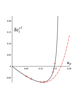
Figure 2: The numerical SF data on $\delta z_{1}^{e^{2}}(u_{p})$ (crosses, extracted by the procedure explained in the text) are compared with two theoretical models: 1) the expression of $\delta z_{1}^{e^{2}}(u_{p})$ in terms of the SF-data-based analytical fits of the EOB potentials $a(u_{p})$ and $\bar{d}(u_{p})$ (solid curve) and 2) the 6.5PN expression of $\delta z_{1}^{e^{2}}(u_{p})$ derived here (dashed curve). Error bars on the numerical data are too small to be visible on this scale.

The latter figure makes very clear two facts: (i) there is a good agreement between the numerically extracted $\delta z_{1}^{e^{2}}$ and the theoretical model incorporating both the theoretical link between EOB theory and $\delta z_{1}^{e^{2}}$ and the current best SF-based representations of the two EOB potentials $a(u)$ and $\bar{d}(u)$; (ii) though the 6.5PN-accurate expansion of $\delta z_{1}^{e^{2}}(u_{p})$, Eq. (24), is in good agreement with the numerically extracted data for $u_{p}\lesssim 0.1$ ($p\gtrsim 10$), it fails to capture the numerical data as one approaches the LSO. Furthermore, it is interesting to note that our first theoretical estimate correctly predicts a change of sign of $\delta z_{1}^{e^{2}}(u_{p})$ between $u_{p}=1/7$ and $u_{p}=1/6.7$. More precisely our first theoretical model predicts that $\delta z_{1}^{e^{2}}(u_{p})$ should vanish at $u_{p}=1/p=1/6.760$. It would be interesting to check this prediction by doing SF simulations with $p=6.760$.

It is important to note that this change of sign close to the LSO is a simple consequence of the singular behavior of the function $\delta z_{1}^{e^{2}}(u)$ near $u=1/6$. Indeed, from Eq. (5.26) of Ref. Tiec:2015cxa follows several facts. First, $\delta z_{1}^{e^{2}}(u)$ can be expressed as the sum of three contributions, namely

$$\delta z_{1}^{e^{2}}(u)=\delta z_{1}^{e^{2}}{}_{\rm hom}(u)+\delta z_{1}^{e^{2}}{}_{a}(u)+\delta z_{1}^{e^{2}}{}_{\bar{d}}(u)\,.$$ (40)

Here the first “homogeneous” contribution is defined as the expression that would remain if $a(u)$ and $\bar{d}(u)$ were set to zero. The second term $\delta z_{1}^{e^{2}}{}_{a}(u)$ is a linear combination of $a(u)$ and its first two derivatives. Finally, the third term $\delta z_{1}^{e^{2}}{}_{\bar{d}}(u)$ is proportional to $\bar{d}(u)$. It easily seen that $\delta z_{1}^{e^{2}}{}_{\bar{d}}(u)$ vanishes at the LSO proportionally to $(1-6u)\bar{d}(u)$. The contribution $\delta z_{1}^{e^{2}}{}_{\rm hom}(u)$ is regular and nonvanishing at the LSO. By contrast, the contribution $\delta z_{1}^{e^{2}}{}_{a}(u)$ diverges at the LSO $\propto(1-6u)^{-1}$. [We are using here the fact that EOB theory predicts that the various EOB potentials are regular at the LSO. Their first singularity is located at the light-ring $u=1/3$ Akcay:2012ea .] This means that we can theoretically predict the singular behavior at the LSO of the full $\delta z_{1}^{e^{2}}(u)$ from the sole knowledge of the main EOB potential $a(u)$. Using as above model 14 of Ref. Akcay:2012ea we explicitly find the following singular behavior

$$\delta z_{1}^{e^{2}\rm th}(u)=\frac{c_{-1}}{1-6u}+c_{0}+O(1-6u)\,,$$ (41)

with the following numerical values

$$c_{-1}\simeq+0.0136455\,\qquad c_{0}\simeq-0.116733\,.$$ (42)

The fact that $c_{-1}$ is positive then predicts that $\delta z_{1}^{e^{2}}(u)=-u+O(u^{2})$ which is negative in the weak-field domain ($u\ll 1$) must change sign before reaching the LSO, thereby explaining the change of sign found above. Let us mention the simple link existing between $\delta z_{1}^{e^{2}}(u)$ and the function $\rho(u)$ (introduced in Damour:2009sm ) measuring the precesssion of small eccentricity orbits. Eliminating $\bar{d}(u)$ between Eq. (36) and the similar expression, derived in Damour:2009sm , linking $\rho(u)$ to $\bar{d}(u)$, $a(u)$, $a^{\prime}(u)$ and $a^{\prime\prime}(u)$ we find

$$\rho(u) = 4u+2\frac{1-2u}{u}\sqrt{1-3u}\delta z_{1}^{e^{2}}(u)$$ (43)

$$+2(1-10u+22u^{2})\sqrt{1-3u}\times$$

$$\left[\frac{1}{1-6u}\frac{d}{du}\left(\frac{a(u)}{\sqrt{1-3u}}\right)+\frac{1-2u}{(1-3u)^{2}}\right]\,.$$

As $\rho(u)$ is a regular function near the LSO this relation shows that the origin of the LSO-singular behavior of $\delta z_{1}^{e^{2}}(u)$ is the term

$$\delta z_{1}^{e^{2}}(u) = -\frac{u(1-10u+22u^{2})}{(1-2u)(1-6u)}\frac{d}{du}\left(\frac{a(u)}{\sqrt{1-3u}}\right)$$ (44)

$$+\hbox{\rm LSO-regular}\,.$$

VI Going beyond the $O(e^{2})$-level

VI.1 Comparison with $O(e^{4})$ information extracted from SF results

We have indicated above how we extracted the $O(e^{2})$ contribution $\delta z_{1}^{e^{2}}(u)$ to $\delta z_{1}(p,e)$ from a part of the data listed in Table IV of Barack:2011ed . The procedure we used, based on representing the subtracted and rescaled data $\widehat{\delta z_{1}}$, Eq. (39), either as $a+be^{2}$ or $a^{\prime}+b^{\prime}e^{2}+c^{\prime}e^{4}$ gives also an estimate of the $O(e^{4})$ contribution $\delta z_{1}^{e^{4}}(u)$ to $\delta z_{1}(p,e)$, namely the value of $b$. In addition, the difference $|b^{\prime}-b|$ gives an estimate of the error bar on $\delta z_{1}^{e^{4}}(u)$. The resulting numerically extracted estimates of $\delta z_{1}^{e^{4}}(u_{p})$ (with their error bars) are displayed in the first column of Table III.

Table 3: Numerical/theoretical comparison for $\delta z_{1}^{e^{4}}$.

$p$	$\delta z_{1}^{e^{4}\rm num}$	$\delta z_{1}^{e^{4}\rm PN}$
20	-0.0036(1)	-0.00334554
15	-0.0072(3)	-0.00668353
10	-0.021(1)	-0.0193812
9	-0.027(1)	-0.0261540
7	+0.03(2)	-0.0561272
6.7	+0.3(2)	-0.0646171

In the second column of the latter table we compare the so extracted numerical estimates to the values of $\delta z_{1}^{e^{4}}(u_{p})$ predicted by the straightforward PN expansion, Eq. (25), deduced from the 4PN knowledge of $q(u)$, Damour:2015isa , together with the results of Ref. Tiec:2015cxa . [Because of the four derivatives of $a(u)$ entering Eq. (5.27) there we found that the use of model 14 leads to inaccuracies too large for getting reliable results.] It is satisfactory to notice that the theoretical estimates are compatible within about twice the indicated error bars for all points except for the last two (near LSO) ones. This indicates that with the present data it seems rather difficult to extract accurate strong-field information going beyond the current theoretical knowledge of $\delta z_{1}^{e^{4}}(u_{p})$.

VI.2 Comparison with SF results on eccentric orbits

In an attempt to bypass the difficulty of decomposing the numerical function $\delta z_{1}(p,e)$ (or for that matter $\delta U(p,e)$) into various powers of $e^{2}$ we also performed direct comparisons between numerical data on $\delta U(p,e)$ and the combined theoretical result obtained by summing: (i) model 14 for $\delta U(p,e=0)$; (ii) our 6.5PN-accurate result, Eq. (18) for the $e^{2}$ contribution, (iii) the 4PN-accurate result, Eq. (19), deduced above and (iv) the 3PN terms for the $e^{6}$ contribution given in Eq. (4.53d) of Ref. Akcay:2015pza . Such a comparison is done in Fig. 3 using as numerical data points a sample of the SF data recently computed in Ref. vandeMeent:2015lxa . The agreement exhibited in Fig. 3 is rather satisfactory and confirms the difficulty in extracting from numerical data information beyond the current theoretical knowledge.

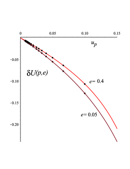
Figure 3: Numerical SF data points (from Ref.Akcay:2015pza ) for $\delta U(p,e)$ are compared with the sum of $\delta U(p,0)$ (given by model 14 in Akcay:2012ea ) and of the PN-expanded analytical prediction of Eqs. (18), (19), (20). We consider the two extreme eccentricities listed in Table II of Akcay:2015pza , namely $e=0.05$ and $e=0.4$.

VII Conclusions

Let us summarize our main results.

The gauge-invariant self-force $O(m_{1}/m_{2})$ correction $\delta U$ to the averaged inverse redshift function $U(m_{2}\Omega_{r},m_{2}\Omega_{\phi},m_{1}/m_{2})=\oint dt/\oint d\tau$ along an eccentric orbit around a Schwarzschild black hole can be viewed as a function of the (dimensionless) semi-latus rectum $p$ and the eccentricity $e$ of the (unperturbed) orbit. The function $\delta U(p,e)$ can be expanded in powers of $e^{2}$: $\delta U(p,e)=\delta U^{e^{0}}(u_{p})+e^{2}\delta U^{e^{2}}(u_{p})+e^{4}\delta U^{e^{4}}(u_{p})+e^{6}\delta U^{e^{6}}(u_{p})+\ldots$, where $u_{p}=1/p$. We computed, by a direct analytic self-force computation along slightly eccentric orbits, the PN-expansion of the term $\delta U^{e^{2}}(u_{p})$ up to order $O(u_{p}^{15/2})$ included (corresponding to the 6.5PN level), see Eq. (18). We completed this result by giving the 4PN-accurate expansion of $\delta U^{e^{4}}(u_{p})$, Eq. (19), deduced by inserting the 4PN Hamiltonian of Damour:2015isa into the relations recently derived in Tiec:2015cxa . [The present knowledge of the next term $\delta U^{e^{6}}(u_{p})$ is limited at the 3PN-level, Eq. (19), see Ref. Akcay:2015pza .] We gave the corresponding results for the self-force correction $\delta z_{1}=-U^{-2}\delta U$ to the averaged redshift $z_{1}=1/U=\oint d\tau/\oint dt$, see Eqs. (24) and (25).

Using the relations derived in Tiec:2015cxa , we converted our 6.5PN expansion of $\delta U^{e^{2}}$ into the corresponding 6.5PN-accurate expansion of the $O(\nu)$ contribution to $\bar{d}(u)$ to the second radial EOB potential $\bar{D}(u;\nu)=1+\nu\bar{d}(u)+O(\nu^{2})$ (which enters the dynamics of eccentric orbits at the $p_{r}^{2}$ level), see Eq. (26).

The 4PN-level comparison between the latter result and the recently derived 4PN-accurate EOB Hamiltonian Damour:2015isa , has given us the first independent analytic confirmation of the 4PN dynamics beyond the limit of circular orbits. We also showed that recent numerical computations of self-force effects along eccentric orbits vandeMeent:2015lxa gave two more (numerical) confirmations of the 4PN dynamics, at the $O(e^{2})$, and at the $O(e^{4})$ levels, see Eqs. (29) and (30) and Eqs. (32) and (33). The same numerical computations gave a further rough confirmation of the 5PN contribution to our 6.5PN $O(e^{2})$ result, see Eqs. (35) and (36). Finally, we pointed out that our result has also confirmed the recent calculation of the 5.5PN contribution to the $O(e^{2})$ dynamics achieved in Damour:2015isa .

In addition to confirming and extending various post-Newtonian and effective-one-body results describing the dynamics of eccentric orbits, we have directly compared our high-order analytic results to various numerical calculations of self-force effects in eccentric orbits Barack:2010ny ; Barack:2011ed ; Akcay:2012ea ; vandeMeent:2015lxa ; Akcay:2015pza . The results of our comparisons are displayed in Figs. 1, 2 and 3 and in Tables II and III. This comparison shows that our high PN order results accurately agree with numerical results up to gravitational potentials $u\leq 0.1$ (corresponding to semi-latus recta $p\leq 10$). On the other hand, in the strong-field domain $0.1\simeq u\simeq\frac{1}{6}$, a good agreement with the recent eccentric redshift self-force data is reached (as illustrated in Fig. 2) only if one replaces the current 6.5PN expanded analytic knowledge of $O(e^{2})$ effects by combining EOB theory (which describes $O(e^{2})$ effects by the secondary potential $\bar{d}(u)$) with analytic fits of the EOB potential $\bar{d}(u)$ obtained from previous numerical self-force data on the precession of small-eccentricity orbits Barack:2010ny ; Akcay:2012ea .

We hope that our new, analytic 6.5PN $O(e^{2})$ results will help to extract more information from numerical self-force calculations both at the order $O(e^{2})$ and at higher orders in $e^{2}$. From the point of view of EOB theory (and of its application to comparable-mass binaries) it would be most useful to extract information about the third $O(\nu)$ EOB radial potential (beyond $a(u)$ and $\bar{d}(u)$), namely the function $q(u)$ entering $O(e^{4})$ effects. The preliminary analysis we presented in Section VI A indicates what is needed for this. One would need a denser set of dedicated self-force computations containing, for various values of $u_{p}=1/p$ uniformly (except for an increased density near $1/6$) covering the interval $0\leq u_{p}\leq 1/6$, a set of small-enough eccentricity values able to accurately extract the coefficient of the $O(e^{4})$ contribution to $\delta z_{1}(p,e)$.

In this respect, let us end by commenting on the analytic structure of the function $\delta z_{1}(p,e)$. Note, first, that when expanding $\delta z_{1}(p,e)$ in powers of $e^{2}$, the coefficients of the successive powers of $e^{2}$ have an increasingly singular behavior near the last stable orbit (LSO) at $p=6$. To start with, $\delta z_{1}^{e^{0}}(p)=\delta z_{1}(p,e=0)$ is regular at the LSO (as follows, say, from its EOB link with the first $O(\nu)$ EOB potential $a(u)$ whose first singularity is at the light-ring Akcay:2012ea . Then, the $O(e^{2})$ piece $\delta z_{1}^{e^{2}}(u_{p})$ has a $\sim 1/(1-6u_{p})$ singularity at the LSO. We numerically computed in Eqs. (41) and (42) the values of the first two coefficients of the Laurent expansion of $\delta z_{1}^{e^{2}}(u)$ deduced from the knowledge of the EOB $O(\nu)$ potential $a(u)$. [We note in passing that it would be interesting to numerically check the predictions (41) and (42) as well as the value $p_{0}=6.760$, we estimated, where $\delta z_{1}^{e^{2}}(1/p)$ vanishes before growing towards $+\infty$ as $p\to 6$.] The corresponding Laurent expansion of the $O(e^{2})$ piece $\delta U^{e^{2}}(u)$ in $\delta U(p,e)$ reads

$$\delta U^{e^{2}}(u)\simeq-\frac{0.05196}{1-6u}+0.5717\,.$$ (45)

Note that the presence of a $\sim 1/(1-6u)$ singularity in $\delta z_{1}^{e^{2}}(u)$ is particularly clear from the link Eq. (43) between the $O(e^{2})$ precession function $\rho(u)$ (introduced in Damour:2009sm and defined there so as to be regular across the LSO), $\delta z_{1}^{e^{2}}(u)$ and $a(u)$: see Eq. (44).

The $O(e^{4})$ piece $\delta z_{1}^{e^{4}}(u)$ has, as a consequence of Eqs. (5.26) and (5.27) in Tiec:2015cxa , a link to the first three $O(\nu)$ EOB potentials of the type

$$\delta z_{1}^{e^{4}}(u)=\delta z_{1}^{e^{4}}{}_{\rm hom}(u)+\delta z_{1}^{e^{4}}{}_{a}(u)+\delta z_{1}^{e^{4}}{}_{\bar{d}}(u)+\delta z_{1}^{e^{4}}{}_{q}(u)\,.$$ (46)

Note that, as in Eq. (40), the first “homogeneous” contribution is analytically known (and LSO-regular); the second term is a linear combination of $a(u)$ and its first four derivatives; the third term is a linear combination of $\bar{d}(u)$ and its first two derivatives; while the fourth and last term is proportional to $q(u)$ and explicitly given by

$$\delta z_{1}^{e^{4}}(u)=9\frac{u^{2}(1-6u)^{2}}{(1-2u)^{4}(1-3u)^{3/2}}q(u)\,.$$ (47)

We only know the 4PN level expansion of the EOB potential $q(u)$ Damour:2015isa , $q(u)=c_{2}u^{2}+c_{3}u^{3}$ (see Eq. (8.1c) in Damour:2015isa ) and, in particular we do not know the value of $q(u)$ at the LSO (besides the fact that the EOB theory predicts that $q(u)$ is regular near the LSO). We see, however, from Eq. (47), that, near the LSO, the effect of $q(u)$ is $O((1-6u)^{2})$. On the other hand, the terms $\delta z_{1}^{e^{4}}{}_{a}$ and $\delta z_{1}^{e^{4}}{}_{\bar{d}}$ involve LSO-singular terms of the symbolic type (indicating only the power of the LSO singulariy)

$$\delta z_{1}^{e^{4}}{}_{a} \sim \frac{a(u)}{(1-6u)^{3}}+\frac{a^{\prime}(u)}{(1-6u)^{3}}+\frac{a^{\prime\prime}(u)}{(1-6u)^{2}}$$

$$+ \frac{a^{\prime\prime\prime}(u)}{(1-6u)}$$

$$\delta z_{1}^{e^{4}}{}_{\bar{d}} \sim \frac{\bar{d}(u)}{(1-6u)}\,.$$ (48)

Using the model 14 analytic fit of $a(u)$ Akcay:2012ea together with our Padé like fit, Eq. (38), for $\bar{d}(u)$ (which, according to Fig. 1 b seems to better capture the LSO behavior of $\bar{d}(u)$), we deduce, from Eqs. (46) and (47), that the theoretically predicted LSO behavior of $\delta z_{1}^{e^{4}}(u)$ is of the type

$$\delta z_{1}^{e^{4}}(u) = \frac{c^{\prime}_{-3}}{(1-6u)^{3}}+\frac{c^{\prime}_{-2}}{(1-6u)^{2}}+\frac{c^{\prime}_{-1}}{(1-6u)}+c^{\prime}_{0}$$ (49)

$$+ c^{\prime}_{1}(1-6u)+O((1-6u)^{2})\,,$$

with the following approximate numerical values for the various coefficients of the Laurent expansion

$$c^{\prime}_{-3} \simeq +0.0004264$$

$$c^{\prime}_{-2} \simeq -0.001279$$

$$c^{\prime}_{-1} \simeq +0.0006447$$

$$c^{\prime}_{0} \simeq -0.09396$$

$$c^{\prime}_{1} \simeq +0.3435\,.$$ (50)

It would be interesting to confirm this prediction by means of dedicated, near LSO, numerical self-force computations.

Summing the various pieces of $\delta z_{1}(p,e)=\delta z_{1}^{e^{0}}(p)+e^{2}\delta z_{1}^{e^{2}}(p)+\ldots$ the structure of the $e^{2}$-dependence of the LSO-singular behavior of $\delta z_{1}(p,e)$ is essentially of the type

$$\delta z_{1}(p,e)\sim 1+\frac{e^{2}}{p-6}+\frac{e^{4}}{(p-6)^{3}}+O(e^{6})\,.$$ (51)

The reason why the $O(e^{4})$ term is more LSO-singular than the square of the $O(e^{2})$ term, is that one should understand this structure as being of the type

$$\delta z_{1}(p,e) = \delta z_{1}(p,0)+\frac{4e^{2}}{p-6}f_{p}(\epsilon)$$ (52)

$$= \delta z_{1}(p,0)+(p-6)\epsilon f_{p}(\epsilon)$$

where

$$\epsilon\equiv\left(\frac{2e}{p-6}\right)^{2}\equiv\left(\frac{e}{e_{c}(p)}\right)^{2}$$ (53)

and where

$$f_{p}(\epsilon)=f_{0}(p)+f_{1}(p)\epsilon+f_{2}(p)\epsilon^{2}+\ldots+f_{2n}\epsilon^{2n}$$ (54)

is a function of $\epsilon$ which is analytic near $\epsilon=0$. [Here, and henceforth, we focus on the $\epsilon$-dependence of $f_{p}(\epsilon)$, which, after the factorizations done in Eq. (52) should be a regular function of $p$ near the LSO]. Indeed, $z_{1}(m_{2}\Omega_{r},m_{2}\Omega_{\phi})$ (and therefore $\delta z_{1}(p,e)$) is an even function of $e$, whose singularities in the complex $e$-plane lie on the two boundaries of the inequalities (8), namely at $e=e_{c}(p)\equiv\frac{p-6}{2}$ and $e=1$. For discussing the singularity structure of the small-$e^{2}$ expansion of $\delta z_{1}(p,e)$, it is the first, “separatrix” boundary, $e=\frac{p-6}{2}$ which matters. This boundary corresponds to a locus where the definition of the function $z_{1}(p,e;\lambda)$, with $\lambda=m_{1}/m_{2}$ [here considered as a function of some exactly defined versions of $p$ and $e$, say through (gauge-invariant) EOB theory] breaks down because of the disappearance of stable bound orbits oscillating between $r_{\rm peri}=Mp/(1+e)$ and $r_{\rm apo}=Mp/(1-e)$. In general mathematical terms, one can view the function $z_{1}(p,e;\lambda)$ as a “period” kont over a cycle. This period becomes singular (as well as its derivative with respect to the small deformation parameter $\lambda=m_{1}/m_{2}$) when the cycle ceases to exist, or abruptly changes character. For a given value of $p$, the change of nature of the cycle (between $r_{\rm peri}$ and $r_{\rm apo}$) happens at min$(e_{c}(p),1)$. When $p<8$, one first encounters the singularity at $e=e_{c}(p)=(p-6)/2$. Viewing the function $f(\epsilon)$ in Eq. (52) as an analytic function in the complex $\epsilon$-plane, the location of the first singularity determines the radius of convergence of its Taylor expansion around $\epsilon=0$. In view of the definition, Eq. (53), of $\epsilon$ this singularity (if $p<8$) is located at $\epsilon=1$. We therefore expect the expansion (54) to have a radius of convergence equal to 1, i.e., that the rescaled expansion coefficients $f_{n}/f_{0}$ are (roughly) of order unity. These considerations give a guideline for choosing, for each value of $p$, the value of $e$ one should explore. Essentially, one wants (at least to explore the near-LSO region $6<p<8$) to have a sample of values of $\epsilon$ (with $0<\epsilon<1$) which is sufficiently dense and uniform (and sufficiently close to $0$) to be able to numerically extract the values of the expansion coefficients $f_{0}(p)$, $f_{1}(p)$, …. The coefficient $f_{0}(p)$ parametrizes $\delta z_{1}^{e^{2}}(p)$ (and therefore $\bar{d}(u_{p})$), while the coefficient $f_{1}(p)$ parametrizes $\delta z_{1}^{e^{4}}(p)$ (and therefore $q(u_{p})$), etc. Such a procedure might help to extract the strong-field behavior of the EOB potential $q(u)$. [Actually, as discussed in Damour:2015isa , $q(u)=q_{4}(u)$ is only the first element in a sequence $q_{4}(u)$, $q_{6}(u)$, $q_{8}(u)$,… parametrizing the coefficients of $p_{r}^{4}$, $p_{r}^{6}$, $p_{r}^{8}$, …. This sequence is in correspondence with $f_{0}(u_{p})$, $f_{1}(u_{p})$, $f_{2}(u_{p})$,…]

To conclude, let us emphasize that studies of the $e^{2}$-expansion of $\delta z_{1}(p,e)$ have the defect of being able to explore the two-body dynamics behind it (say in its EOB formulation to be concrete) only in the medium-strong-field domain $0<u<\frac{1}{6}$. It cannot access the really strong-field domain $\frac{1}{6}\leq u<\frac{1}{3}$ where the various $O(\nu)$ EOB potentials are a priori defined and regular. In view of this limitation, we recommend that the self-force community make an effort to implement the suggestions made in Ref. Damour:2009sm . Indeed, Damour:2009sm (notably see Sec. VI there) suggested several different ways of extracting gauge-invariant information from self-force theory that might be useful for informing the dynamics of comparable-mass binaries (notably in its EOB formulation). In particular, Damour:2009sm suggested to compute the gauge-invariant functional link $\theta({\mathcal{E}},J)$ between the (total, conserved) energy ${\mathcal{E}}$ and angular momentum $J$ and the scattering angle $\theta$ of hyperbolic-like orbits. To avoid having to correct for the effect of the radiation-damping part of the self-force (though an appropriate method for doing so was provided in Bini:2012ji ) it would be best to compute the function $\theta_{\rm cons}({\mathcal{E}},J)$ associated with the conservative part of the self-force. As mentioned in Damour:2009sm , the function of two variables $\theta_{\rm cons}({\mathcal{E}},J)$ contains “ample information for determining the functions entering the EOB formalism.” We note in particular here that this function has the potential of probing the functions $\bar{d}(u)$, $q_{2n}(u)$ in the full strong-field domain $0<u<\frac{1}{3}$. This information would usefully complement the recent work Damour:2014afa which succeeded in probing the dynamics of comparable-mass binaries by extracting $\theta({\mathcal{E}},J)$ from full numerical relativity simulations of hyperbolic-like close binary black hole encounters.

Acknowledgments

We thank Seth Hopper for attracting our attention to Ref. vandeMeent:2015lxa . D.B. thanks the Italian INFN (Naples) for partial support and IHES for hospitality during the development of this project. All the authors are grateful to ICRANet for partial support.

References

- (1) A. Buonanno and T. Damour, “Effective one-body approach to general relativistic two-body dynamics,” Phys. Rev. D 59, 084006 (1999) [gr-qc/9811091].
- (2) A. Buonanno and T. Damour, “Transition from inspiral to plunge in binary black hole coalescences,” Phys. Rev. D 62, 064015 (2000) [gr-qc/0001013].
- (3) T. Damour, P. Jaranowski and G. Schaefer, “On the determination of the last stable orbit for circular general relativistic binaries at the third postNewtonian approximation,” Phys. Rev. D 62, 084011 (2000) [gr-qc/0005034].
- (4) T. Damour, “Coalescence of two spinning black holes: an effective one-body approach,” Phys. Rev. D 64, 124013 (2001) [gr-qc/0103018].
- (5) G. Schaefer, “Post-Newtonian methods: Analytic results on the binary problem,” Fundam. Theor. Phys. 162, 167 (2011) [arXiv:0910.2857 [gr-qc]].
- (6) L. Blanchet, “Gravitational Radiation from Post-Newtonian Sources and Inspiralling Compact Binaries,” Living Rev. Rel. 17, 2 (2014) [arXiv:1310.1528 [gr-qc]].
- (7) L. Barack, “Gravitational self force in extreme mass-ratio inspirals,” Class. Quant. Grav. 26, 213001 (2009) [arXiv:0908.1664 [gr-qc]].
- (8) E. Poisson, A. Pound and I. Vega, “The Motion of point particles in curved spacetime,” Living Rev. Rel. 14, 7 (2011) [arXiv:1102.0529 [gr-qc]].
- (9) S. L. Detweiler, “A Consequence of the gravitational self-force for circular orbits of the Schwarzschild geometry,” Phys. Rev. D 77, 124026 (2008) [arXiv:0804.3529 [gr-qc]].
- (10) L. Barack and N. Sago, “Beyond the geodesic approximation: conservative effects of the gravitational self-force in eccentric orbits around a Schwarzschild black hole,” Phys. Rev. D 83, 084023 (2011) [arXiv:1101.3331 [gr-qc]].
- (11) A. Le Tiec, “First Law of Mechanics for Compact Binaries on Eccentric Orbits,” Phys. Rev. D 92, no. 8, 084021 (2015) [arXiv:1506.05648 [gr-qc]].
- (12) S. Akcay, L. Barack, T. Damour and N. Sago, “Gravitational self-force and the effective-one-body formalism between the innermost stable circular orbit and the light ring,” Phys. Rev. D 86, 104041 (2012) [arXiv:1209.0964 [gr-qc]].
- (13) E. Barausse, A. Buonanno and A. Le Tiec, “The complete non-spinning effective-one-body metric at linear order in the mass ratio,” Phys. Rev. D 85, 064010 (2012) [arXiv:1111.5610 [gr-qc]].
- (14) T. Damour and G. Schaefer, “Higher Order Relativistic Periastron Advances and Binary Pulsars,” Nuovo Cim. B 101, 127 (1988).
- (15) P. Jaranowski and G. Schaefer, “Dimensional regularization of local singularities in the 4th post-Newtonian two-point-mass Hamiltonian,” Phys. Rev. D 87, 081503 (2013) [arXiv:1303.3225 [gr-qc]].
- (16) D. Bini and T. Damour, “Analytical determination of the two-body gravitational interaction potential at the fourth post-Newtonian approximation,” Phys. Rev. D 87, no. 12, 121501 (2013) [arXiv:1305.4884 [gr-qc]].
- (17) T. Damour, P. Jaranowski and G. Schaefer, “Nonlocal-in-time action for the fourth post-Newtonian conservative dynamics of two-body systems,” Phys. Rev. D 89, no. 6, 064058 (2014) [arXiv:1401.4548 [gr-qc]].
- (18) P. Jaranowski and G. Schaefer, “Derivation of the local-in-time fourth post-Newtonian ADM Hamiltonian for spinless compact binaries,” arXiv:1508.01016 [gr-qc].
- (19) T. Damour, P. Jaranowski and G. Schaefer, “Fourth post-Newtonian effective one-body dynamics,” Phys. Rev. D 91, no. 8, 084024 (2015) [arXiv:1502.07245 [gr-qc]].
- (20) M. van de Meent and A. G. Shah, “Metric perturbations produced by eccentric equatorial orbits around a Kerr black hole,” Phys. Rev. D 92, no. 6, 064025 (2015) [arXiv:1506.04755 [gr-qc]].
- (21) S. Akcay, A. Le Tiec, L. Barack, N. Sago and N. Warburton, “Comparison Between Self-Force and Post-Newtonian Dynamics: Beyond Circular Orbits,” Phys. Rev. D 91, no. 12, 124014 (2015) [arXiv:1503.01374 [gr-qc]].
- (22) L. Barack, T. Damour and N. Sago, “Precession effect of the gravitational self-force in a Schwarzschild spacetime and the effective one-body formalism,” Phys. Rev. D 82, 084036 (2010) [arXiv:1008.0935 [gr-qc]].
- (23) T. Damour, “Gravitational Self Force in a Schwarzschild Background and the Effective One Body Formalism,” Phys. Rev. D 81, 024017 (2010) [arXiv:0910.5533 [gr-qc]].
- (24) T. Damour and N. Deruelle, “General relativistic celestial mechanics of binary systems I. The post-Newtonian motion. ” Ann. Inst. Henri Poincaré 43, 107 (1985).
- (25) T. Damour and N. Deruelle, “General relativistic celestial mechanics of binary systems II. The post-Newtonian timing formula.” Ann. Inst. Henri Poincaré, 44, 263 (1986)
- (26) D. Bini and T. Damour, “High-order post-Newtonian contributions to the two-body gravitational interaction potential from analytical gravitational self-force calculations,” Phys. Rev. D 89, no. 6, 064063 (2014) [arXiv:1312.2503 [gr-qc]].
- (27) S. Mano, H. Suzuki and E. Takasugi, “Analytic solutions of the Regge-Wheeler equation and the postMinkowskian expansion,” Prog. Theor. Phys. 96, 549 (1996) [gr-qc/9605057].
- (28) S. Mano, H. Suzuki and E. Takasugi, “Analytic solutions of the Teukolsky equation and their low frequency expansions,” Prog. Theor. Phys. 95, 1079 (1996) [gr-qc/9603020].
- (29) D. Bini and T. Damour, “Detweiler s gauge-invariant redshift variable: Analytic determination of the nine and nine-and-a-half post-Newtonian self-force contributions,” Phys. Rev. D 91, 064050 (2015) [arXiv:1502.02450 [gr-qc]].
- (30) C. Kavanagh, A. C. Ottewill and B. Wardell, “Analytical high-order post-Newtonian expansions for extreme mass ratio binaries,” Phys. Rev. D 92, no. 8, 084025 (2015) [arXiv:1503.02334 [gr-qc]].
- (31) L. Blanchet, S. L. Detweiler, A. Le Tiec and B. F. Whiting, “High-Order Post-Newtonian Fit of the Gravitational Self-Force for Circular Orbits in the Schwarzschild Geometry,” Phys. Rev. D 81, 084033 (2010) [arXiv:1002.0726 [gr-qc]].
- (32) M. Kontsevich and D. Zagier, “Periods,” in B. Engquist, W. Schmid, Mathematics unlimited 2001 and beyond, Berlin, New York: Springer-Verlag, pp. 771 808 (2001).
- (33) D. Bini and T. Damour, “Gravitational radiation reaction along general orbits in the effective one-body formalism,” Phys. Rev. D 86, 124012 (2012) [arXiv:1210.2834 [gr-qc]].
- (34) T. Damour, F. Guercilena, I. Hinder, S. Hopper, A. Nagar and L. Rezzolla, “Strong-Field Scattering of Two Black Holes: Numerics Versus Analytics,” Phys. Rev. D 89, no. 8, 081503 (2014) [arXiv:1402.7307 [gr-qc]].