High-order-harmonic generation in benzene with linearly and circularly polarised laser pulses

Abstract

High-order-harmonic generation in benzene is studied using a mixed quantum-classical approach in which the electrons are described using time-dependent density functional theory while the ions move classically. The interaction with both linearly and circularly polarised infra-red ($\lambda=800$ nm) laser pulses of duration 10 cycles (26.7 fs) is considered. The effect of allowing the ions to move is investigated as is the effect of including self-interaction corrections to the exchange-correlation functional. Our results for circularly polarised pulses are compared with previous calculations in which the ions were kept fixed and self-interaction corrections were not included while our results for linearly polarised pulses are compared with both previous calculations and experiment. We find that even for the short duration pulses considered here, the ionic motion greatly influences the harmonic spectra. While ionization and ionic displacements are greatest when linearly polarised pulses are used, the response to circularly polarised pulses is almost comparable, in agreement with previous experimental results.

I Introduction

High-order-harmonic generation (HHG) is a highly non-linear process which occurs when intense, short-duration laser pulses interact with targets such as atomic or molecular gases Bandrauk et al. (2007). The study of HHG in these systems has attracted much experimental and theoretical attention in recent years since it represents a mechanism for the production of attosecond laser pulses and can also be used as a probe to study how the target atoms or molecules respond during the interaction Ferré et al. (2015); Wong et al. (2011); Cireasa et al. (2015).

Of particular interest is understanding the response of molecules to intense laser pulses. This interest arises from the many degrees of freedom that molecules possess which leads to a richer set of features and processes when compared to the response of atomic gases. Understanding these molecular processes is important since they are crucial in many areas of chemistry and biology. For example, early simulations showed that charge transfer across the molecule can occur on a femtosecond timescale Remacle and Levine (2006). This opens up the possibility of steering electrons in the molecule using attosecond pulses to control the response and possible fragmentation of the molecule Krausz and Ivanov (2009). Due to the extra degrees of freedom we expect that molecular HHG will be highly sensitive to changes in the molecular dynamics.

Most studies of HHG have focussed on the interaction with linearly polarised pulses. In the three-step model an electron is liberated by tunnel ionization and propagates as a free particle in the field before recolliding with the ionic core Corkum (1993); Kulander et al. (1993). For elliptically and circularly polarised light the probability for a direct recollision is greatly reduced – although still present Rajgara et al. (2003); Mauger et al. (2010), and so harmonic generation processes in these fields are distinctly different. Understanding how elliptically and circularly polarised light interacts with molecules is highly important due to the recent experimental and theoretical interest in generating circularly polarised attosecond pulses Ferré et al. (2015) and in studying the interaction of linearly and elliptically polarised pulses with chiral molecules Wong et al. (2011); Cireasa et al. (2015).

A number of theoretical approaches considered molecular HHG in circularly-polarised fields. Alon et al Alon et al. (1998) studied the HHG selection rules that hold when symmetric molecules such as benzene interact with circularly polarised laser fields. For continuous wave circularly polarised pulses that were polarised parallel to the molecular plane, they showed that a $6k\pm 1\,\,(k=0,1,2,\dots)$ symmetry rule held. Averbuch et al Averbukh et al. (2001) then showed that HHG in this case was predomnantly due to bound-bound transitions. This is distinctly different to bound-continuum transitions that drive HHG in the three-step model. Later, Baer et al Baer et al. (2003) considered the interaction of benzene with finite duration, circularly polarised pulses and showed that the $6k\pm 1$ selection rule was still evident, even for short pulses. However, a number of questions remained unanswered in the study of Baer et al. Firstly, their calculations used time-dependent density functional theory (TDDFT) Runge and Gross (1984) in which many-body effects were treated at the level of the local density approximation. It is well known that such an approximation includes self-interaction errors. In particular, the exchange-correlation potential does not have the proper asymptotic form meaning that the ionization potential of the molecule is underestimated. Secondly, their calculations considered the ions to be fixed in space. As mentioned above, HHG is highly sensitive to changes in the molecular response and so the effect of allowing the ions to move, even for such short duration pulses, has not been fully explored.

Describing HHG in complex molecules is theoretically and computationally demanding. The number of degrees of freedom in the problem together with the duration of the laser pulses and the length scales required to describe recolliding electrons means that solution of the time-dependent Schrödinger equation is impractical for all but the simplest one- and two-electron molecules He et al. (2008); Kono et al. (1997); Lein et al. (2003); Dundas et al. (2003); Lein et al. (2003); Bandrauk and Lu (2004); Vanne and Saenz (2010); Kjeldsen et al. (2006); Morales et al. (2014); Hou et al. (2012); Yuan and Bandrauk (2012). For more complex molecules, approximations are required. One successful technique for studying HHG in complex molecules is the strong field approximation (SFA) in which either single or multiple ionic channels can be considered Spanner and Patchkovskii (2009); Smirnova et al. (2009); Cireasa et al. (2015). While this method has allowed HHG in general elliptically polarised laser pulses to be investigated, it does suffer from the drawback that only a small number of channels are generally included in the calculation. This can become an issue, depending on the molecule under investigation, if other channels become important. Indeed, such a situation has been observed in other ab initio calculations in which multiple electrons can contribute to the molecular response Chu and Chu (2004); Dundas and Rost (2005); Fowe and Bandrauk (2011); Petretti et al. (2010). Another successful technique for studying HHG is quantitative rescattering (QRS) theory Le et al. (2009); Lin et al. (2010). In this approach, the induced dipoles can be expressed as the product of a recolliding electronic wavepacket with a photorecombination cross section. Multiple orbitals can be incorporated within QRS and the method has successfully applied to HHG in complex molecules Jin et al. (2011a); Wong et al. (2013); Le et al. (2013a, b). Like the strong-field approximation, the influence of multiple orbitals in QRS can only be studied if they have been included from the outset. One ab initio approach that is widely used for studying laser molecule interactions is TDDFT. While it has mainly been used to study the electronic response Telnov and Chu (2009); Heslar et al. (2011); Fowe and Bandrauk (2011); Petretti et al. (2010); Baer et al. (2003) some implementations combine TDDFT with a classical description of the ionic motion Kunert and Schmidt (2003); Uhlmann et al. (2003); Dundas (2004); Calvayrac et al. (2000); Castro et al. (2004); Dundas (2012). To date, very few implementations combine the treatment of ionic motion with approximations to the exchange-correlation functional that include self-interaction corrections Wopperer et al. (2012); Crawford-Uranga et al. (2014). However, these calculations have generally considered the interaction with high-frequency laser pulses. As far as we are aware, no calculations of HHG in infra-red (IR) pulses have been carried out before that combine moving ions with self-interaction corrections.

In this paper we study HHG in benzene using both circularly and linearly polarised IR laser pulses. We use a mixed quantum-classical approach in which electrons are treated using TDDFT while the ions are described classically. In our treatment, self-interaction corrections to the exchange-correlation functional are included. The paper is arranged as follows. In Sec. II we describe our approach and give details of the numerical methods and parameters used in our simulations. In Sec. III our results are presented. Firstly, we consider benzene interacting with circularly-polarised pulses. The effect of including self-interaction corrections and allowing the ions to move is investigated. Secondly, we show how the response of the molecule changes when linearly polarised pulses are used. In particular, we show that the response of the ions is slightly greater for linearly polarised pulses. Finally, in Sec. IV we present our conclusions and possible directions for future work are highlighted.

Unless otherwise stated, atomic units are used throughout.

II Theoretical Approach

In our calculations we consider quantum mechanical electrons and classical ions interacting with intense, ultra-short laser pulses in a method known as non-adiabatic quantum molecular dynamics (NAQMD). The implementation of this method, in a code called EDAMAME (Ehrenfest DynAMics on Adaptive MEshes), is described in more detail in Ref. Dundas (2012). We now briefly describe how it is applied to the calculations considered here.

We consider $N_{n}$ classical ions where $M_{k}$, $Z_{k}$ and $\mbox{\boldmath$R$}_{k}$ denote respectively the mass, charge and position of ion $k$. Additionally $\mbox{\boldmath$R$}=\{\mbox{\boldmath$R$}_{1},\dots,\mbox{\boldmath$R$}_{N_{n}}\}$. Time dependent density functional theory (TDDFT) Runge and Gross (1984) is used to model the electronic dynamics. Neglecting electron spin effects, the time-dependent electron density can be written in terms of $N$ time-dependent Kohn-Sham orbitals, $\psi_{i}(\mbox{\boldmath$r$},t)$, as

$$n(\mbox{\boldmath$r$},t)=2\sum_{j=1}^{N}\left|\psi_{j}(\mbox{\boldmath$r$},t)\right|^{2}.$$ (1)

These Kohn-Sham orbitals satisfy the time dependent Kohn-Sham equations (TDKS)

$$i\frac{\partial}{\partial t}\psi_{j}(\mbox{\boldmath$r$},t)=\Biggr{[} -\frac{1}{2}\nabla^{2}+V_{\mbox{\scriptsize H}}(\mbox{\boldmath$r$},t)+V_{\mbox{\scriptsize ext}}(\mbox{\boldmath$r$},\mbox{\boldmath$R$},t)$$

$$+V_{\mbox{\scriptsize xc}}(\mbox{\boldmath$r$},t)\Biggr{]}\psi_{j}(\mbox{\boldmath$r$},t)=H_{\mbox{\scriptsize ks}}\psi_{j}(\mbox{\boldmath$r$},t).$$ (2)

In Eq. (2), $V_{\mbox{\scriptsize H}}(\mbox{\boldmath$r$},t)$ is the Hartree potential, $V_{\mbox{\scriptsize ext}}(\mbox{\boldmath$r$},\mbox{\boldmath$R$},t)$ is the external potential, and $V_{\mbox{\scriptsize xc}}(\mbox{\boldmath$r$},t)$ is the exchange-correlation potential. Both the Hartree and exchange-correlation potentials are time-dependent due to their functional dependence on the time-dependent density. The external potential accounts for both electron-ion interactions and the interaction of the laser field with the electrons and can be written as

$$V_{\mbox{\scriptsize ext}}(\mbox{\boldmath$r$},\mbox{\boldmath$R$},t)=V_{\mbox{\scriptsize ions}}(\mbox{\boldmath$r$},\mbox{\boldmath$R$},t)+U_{\mbox{\scriptsize elec}}(\mbox{\boldmath$r$},t).$$ (3)

The calculations presented in this paper will consider the response of benzene to IR laser pulses. In that case the laser will predominately couple to the valence electrons and so we will only consider their response. The electron-ion interactions, $V_{\mbox{\scriptsize ions}}(\mbox{\boldmath$r$},\mbox{\boldmath$R$},t)$, are described with Troullier-Martins pseudopotentials Troullier and Martins (1991) in the Kleinman-Bylander form Kleinman and Bylander (1982). All pseudopotentials were generated using the APE (Atomic Pseudopotentials Engine) Oliveira et al (2008).

Both length and velocity gauge descriptions of the electron-laser interaction, $U_{\mbox{\scriptsize elec}}(\mbox{\boldmath$r$},t)$, can be used by EDAMAME. We use the length gauge description here as it the simpler to implement and major differences between the gauges have not previously been observed Dundas (2012). Working within the dipole approximation we then have

$$U_{\mbox{\scriptsize elec}}(\mbox{\boldmath$r$},t)=U_{L}(\mbox{\boldmath$r$},t)=\mbox{\boldmath$r$}\cdot\mbox{\boldmath$E$}(t).$$ (4)

	Equilibrium bond lengths (a.u.)		Ionization Potential (a.u.)
	C–C bond length	C–H bond length
LDA-PW92	2.622	2.066	0.243
L-ADSIC	2.541	2.138	0.345
Experimental	2.644	2.081	0.340

Table 1: Static properties of benzene. The equilibrium C-C and C-H bond lengths and ionization potential calculated using LDA-PW92 and L-ADSIC are compared with experimental values. The ionization potential is estimated from the Highest occupied molecular orbital (HOMO) orbital energy. Other calculation parameters are detailed in the text. We see that the C-C bond lengths are underestimated with L-ADSIC while the C-H bond lengths are overestimated. However, the ionization potential is much more accurate using L-ADSIC. Experimental bond lengths are taken from Meijer and Sprik (1996) while the ionization potential is taken from Sharifi et al. (2007)

In the calculations presented in the paper we consider benzene interacting with both linearly and circularly polarised pulses. In the case of linearly polarised light, we take the polarisation direction to be along the $x$ axis. In that case, the vector potential has the form

$$\mbox{\boldmath$A$}(t)=A_{0}f(t)\cos(\omega_{L}t+\phi)\mbox{\boldmath$\hat{e}$}_{x}.$$ (5)

Here $A_{0}$ is the peak value of the vector potential, $\omega_{L}$ is the laser frequency, $\phi$ is the carrier-envelope phase and $f(t)$ is the pulse envelope which we model as

$$f(t)=\left\{\begin{matrix}\displaystyle\sin^{2}\left(\frac{\pi t}{T}\right)&0\leq t\leq T\\[11.38092pt] 0&\textup{otherwise}\end{matrix}\right.,$$ (6)

where $T$ is the duration of a pulse. From this, the electric vector is

$$\mbox{\boldmath$E$}(t)=E(t)\mbox{\boldmath$\hat{e}$}_{x},$$ (7)

where

$$E(t)=E_{0}f(t)\sin(\omega_{L}t+\phi)-\frac{E_{0}}{\omega_{L}}\frac{\partial f}{\partial t}\cos(\omega_{L}t+\phi),$$ (8)

and where $E_{0}$ is the peak electric field strength.

For circularly polarised light, we consider the pulse to be polarised in the $x-y$ plane so that the vector potential is given by

$$\mbox{\boldmath$A$}(t) =A_{0}f(t)\Bigr{(}\cos(\omega_{L}t+\phi)\mbox{\boldmath$\hat{e}$}_{x}+\sin(\omega_{L}t+\phi)\mbox{\boldmath$\hat{e}$}_{y}\Bigr{)}$$

$$=A_{x}(t)\mbox{\boldmath$\hat{e}$}_{x}+A_{y}(t)\mbox{\boldmath$\hat{e}$}_{y}.$$ (9)

The pulse envelope takes the form given in Eq. (6). In that case the electric field is given by

$$\mbox{\boldmath$E$}(t)=E_{x}(t)\mbox{\boldmath$\hat{e}$}_{x}+E_{y}(t)\mbox{\boldmath$\hat{e}$}_{y},$$ (10)

where

$$E_{x}(t)=\frac{E_{0}}{\sqrt{2}}f(t)\sin(\omega_{L}t+\phi)-\frac{E_{0}}{\sqrt{2}\omega_{L}}\frac{\partial f}{\partial t}\cos(\omega_{L}t+\phi),$$ (11)

and

$$E_{y}(t)=-\frac{E_{0}}{\sqrt{2}}f(t)\cos(\omega_{L}t+\phi)-\frac{E_{0}}{\sqrt{2}\omega_{L}}\frac{\partial f}{\partial t}\sin(\omega_{L}t+\phi).$$ (12)

The exchange-correlation potential, $V_{\mbox{\scriptsize xc}}(\mbox{\boldmath$r$},t)$, accounts for all electron-electron interactions. The exact form of the exchange-correlation action functional is unknown and so must be approximated. In this paper, we consider two adiabatic approximations to the exchange-correlation potential. In the first approximation, the local density approximation (LDA) incorporating the Perdew-Wang parameterization of the correlation functional is used Perdew and Wang (1992); we will refer to this method as LDA-PW92. The LDA derives from describing the electrons as a homogeneous electron gas. Although LDA is widely used, it has self-interaction errors which means that it does not have the correct long range behaviour. In particular, the exchange-correlation potential decays exponentially instead of Coulombically, meaning that ionization potentials are underestimated. In the second approximation, the LDA-PW92 functional is supplemented by the average density self-interaction correction (ADSIC) Legrand et al (2002); we will refer to this method as L-ADSIC. L-ADSIC aims to correct the self-interaction errors through use of an orbital-independent term involving the average of the total electron density. A major benefit of L-ADSIC is that the exchange-correlation potential can be obtained as the functional derivative of an exchange-correlation functional, meaning that the forces acting on ions can be derived from the Hellmann-Feynman theorem.

We solve the Kohn-Sham equations numerically using finite difference techniques on a three dimensional grid. All derivative operators are approximated using 9-point finite difference rules and the resulting grid is parallelised in 3D. The following mesh parameters were used for the calculations presented in this paper. In those simulations where circularly-polarised pulses were used, the grid extents were $|x|\leq 76.8\,a_{0}$, $|y|\leq 76.8\,a_{0}$ and $|z|\leq 48.8\,a_{0}$ while for linearly-polarised pulses the extents were $|x|\leq 104.8\,a_{0}$, $|y|\leq 62.8\,a_{0}$ and $|z|\leq 62.8\,a_{0}$. A larger grid extent along the laser polarisation direction is used whenever the response to linearly-polarised pulses is considered. This is because we need to handle recolliding wavepackets that travel predominantly in this direction. Grid spacings of $0.4\,a_{0}$ were used for all coordinates.

The ionic dynamics are treated classically using Newton’s equations of motion. For ion $k$ we have

$$M_{k}\ddot{R}_{k}= -\int n(\mbox{\boldmath$r$},t)\frac{\partial H_{\mbox{\scriptsize ks}}}{\partial\mbox{\boldmath$R$}_{k}}\mathrm{d}\mbox{\boldmath$r$}$$

$$-\frac{\partial}{\partial\mbox{\boldmath$R$}_{k}}\Bigr{(}V_{nn}(\mbox{\boldmath$R$})+Z_{k}\mbox{\boldmath$R$}_{k}\cdot\mbox{\boldmath$E$}(t)\Bigr{)},$$ (13)

where $V_{nn}(\mbox{\boldmath$R$})$ is the Coulomb repulsion between the ions and $Z_{k}\mbox{\boldmath$R$}_{k}\cdot\mbox{\boldmath$E$}(t)$ denotes the interaction between ion $k$ and the laser field.

We need to propagate both the TDKS equations, Eq. (2), and ionic equations of motion, Eq. (13), in time. We propagate the TDKS equations using an 18th-order unitary Arnoldi propagator Dundas (2004); Arnoldi (1951); Smyth et al (1998). For the ionic equations of motion, we use the velocity-Verlet method. Converged results are obtained for a timestep of $0.2$ a.u.

As a simulation progresses, electronic wavepackets can travel to the edge of the spatial grid, reflect and travel back towards the molecular centre. These unphysical reflections can be overcome using a wavefunction splitting technique that removes wavepackets that reach the edge of the grid Smyth et al (1998). The splitting is accomplished using a mask function, $M(\mbox{\boldmath$r$})$, that splits the Kohn-Sham orbital, $\psi_{j}(\mbox{\boldmath$r$},t)$, into two parts. One part, $M(\mbox{\boldmath$r$})\psi_{j}(\mbox{\boldmath$r$},t)$, is located near the molecule and is associated with non-ionized wavepackets. The other part, $\left\{1-M(\mbox{\boldmath$r$})\right\}\psi_{j}(\mbox{\boldmath$r$},t)$, is located far from the molecule and is associated with ionizing wavepackets: this part is discarded in our calculations. The point at which we apply this splitting must be be chosen carefully to ensure only ionizing wavepackets are removed. We write the mask function in the form

$$M(\mbox{\boldmath$r$})=M_{x}(x)M_{y}(y)M_{z}(z).$$ (14)

If we consider the $x$ component we can write

$$M_{x}(x)=\left\{\begin{matrix}1&\left|x\right|\leq x_{m}\\[11.38092pt] 1-\alpha\left(\left|x\right|-x_{m}\right)^{5}&\left|x\right|>x_{m}\end{matrix}\right.,$$ (15)

where

$$\alpha=\frac{1-M_{f}}{(x_{f}-x_{m})^{5}}.$$ (16)

Here $x_{m}$ is the point on the grid where the mask starts, $x_{f}$ is the maximum extent of the grid in $x$ and $M_{f}$ is the value that we want the mask function to take at the edges of the grid. Similar descriptions are used for $M_{y}(y)$ and $M_{z}(z)$.

Within TDDFT ionization is a functional of the electronic density. The exact form of this functional is unknown and so most measures of ionization are obtained using geometric properties of the time-dependent Kohn-Sham orbitals Ullrich (2000). In this approach, bound- and continuum-states are separated into different regions of space through the introduction of an analysing box. In principal the continuum states occupy the regions of space when the wavefunction splitting is applied and hence the reduction in the orbital occupancies provides a measure of ionization.

III Results

The starting point for our calculations is to obtain the ground state of benzene. We do this by taking a trial guess for the geometry from the NIST Chemistry WebBook National Institute of Standards and Technology Chemistry WebBook() (NIST). Relaxing this initial structure using the different exchange-correlation potentials gives the equilibrium properties presented in Table 1. We see from these structural properties that the equilibrium geometry is well reproduced using LDA-PW92. Using L-ADSIC we see that the C–C bond lengths are underestimated while the C–H bond lengths are overestimated. This is similar to what is found using other ADSIC calculations Legrand et al (2002). Additionally we see that the ionization potential is better represented using L-ADSIC than that obtained using LDA-PW92. Indeed, if we plot the Kohn-Sham orbital energies, as shown in Fig. 1, we see that L-ADSIC gives a better representation of the electronic structure than LDA-PW92. In particular, we see that several Kohn-Sham orbitals are much more loosely bound when using LDA-PW92.

Figure 1: Kohn-Sham orbital energies of benzene obtained from relaxed geometries using both LDA-PW92 and L-ADSIC approximations to the exchange-correlation functional. The dotted line is plotted at the negative of the experimental ionization potential of benzene. We see that using L-ADSIC the HOMO orbital energy gives a good approximation to this ionization potential.

We are now in a position to consider benzene interacting with intense laser pulses. The first question we can ask is how does the molecule respond to circularly- and linearly-polarised light? We visualise both these situations in Fig. 2. In both simulations the L-ADSIC exchange-correlation potential is used and the ions are allowed to move. The densities presented are obtained by integrating the full 3D density over the $z$ coordinate. Fig. 2(a) presents a snapshot of the electronic density of benzene during its interaction with a 10-cycle linearly-polarised pulse having a peak intensity of $I=$ $2.0\times 10^{14}\mbox{ W/cm}^{2}$ and wavelength of $\lambda=$ 800 nm. The laser is polarised along the $x$-axis. We clearly see that the electronic response is predominantly along this direction. In the frame shown the electron is being forced along the positive $x$-direction. We see electrons streaming outwards in this direction. At small negative $x$ values we can also clearly see ionized electrons recolliding with the parent molecule. For circular polarisation, the situation is markedly different. Here we see electrons spiralling outwards as the molecule responds to the field. While most electrons never return to the parent core, we see some evidence of electron wavepackets ionizing from one atomic centre and subsequently recombining with at an adjacent atomic centre: this is more evident when we consider a movie of the evolving density. Animations of both simulations are presented in the supplementary material.

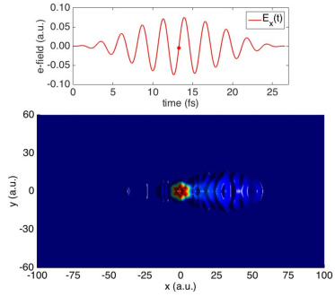
(a)

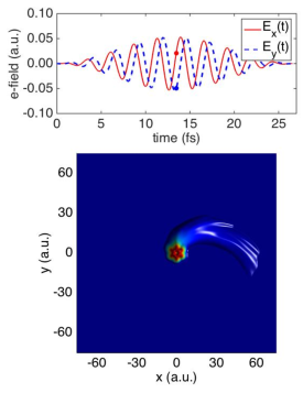
(b)

Figure 2: Snapshots of the electronic density of benzene during interaction with (a) a 10-cycle linearly-polarised pulse having a peak intensity of $2.0\times 10^{14}\mbox{ W/cm}^{2}$ and wavelength of 800 nm and (b) a 10-cycle circularly-polarised pulse having a peak intensity of $2.0\times 10^{14}\mbox{ W/cm}^{2}$ and wavelength of 800 nm. In both cases the L-ADSIC approximation has been used and the ions are allowed to move. The densities presented are obtained by integrating the full 3D density over the $z$ coordinate. The densities are plotted on a logarithmic scale and the lowest density has been clamped to $10^{-4}$.

Now we know that the electronic response is markedly different we can consider ionization, harmonic generation and the response of the ions to the different laser pulses. For HHG, we calculate the spectral density, $S_{k}(\omega)$, along the direction $\hat{\mbox{\boldmath$e$}}_{k}$ from the Fourier transform of the dipole acceleration Burnett et al. (1992)

$$S_{k}(\omega)=\left|\int e^{i\omega t}\,\hat{\mbox{\boldmath$e$}}_{k}\cdot\ddot{\mbox{\boldmath$d$}}(t)\,\mathrm{d}t\right|^{2},$$ (17)

where $\ddot{\mbox{\boldmath$d$}}(t)$ is the dipole acceleration given by

$$\ddot{\mbox{\boldmath$d$}}(t)=-\int n(\mbox{\boldmath$r$},t)\mbox{\boldmath$\nabla$}H_{\mbox{\scriptsize ks}}\mathrm{d}\mbox{\boldmath$r$}.$$ (18)

III.1 Molecular response to circularly-polarised light

Baer et al Baer et al. (2003) studied HHG in benzene with TDDFT using the LDA-PW92 approximation to the exchange-correlation functional. In their work the ions were kept fixed in space and the harmonic response was studied for a range of laser intensities and pulse lengths. Here we are interested in how our results are altered by using a more accurate exchange-correlation functional and allowing the ions to move. Thus we initially consider the interaction with a 10-cycle laser pulse of wavelength $\lambda=$ 800 nm and peak intensity $I=$ $3.5\times 10^{14}\mbox{ W/cm}^{2}$. To compare with Baer et al we will present harmonic spectra for the response in the $x$ direction, i.e. $S_{x}(\omega)$. Figure 3 compares the harmonic spectra when the ions are kept fixed and when they are allowed to move. Both exchange-correlation functionals have been used. Even for these short-duration pulses, we see that the $6k\pm 1,(k=0,1,\dots)$ selection rule holds in all cases, i.e. the 3rd, 9th and 15th harmonics are suppressed. In all cases we can compare the relative strengths of the harmonics obtained. These are presented in the first part of Table (2) where our results are compared with those of Baer et al Baer et al. (2003). Our results show that the relative strengths change greatly depending on the exchange-correlation functional used and whether or not the ions are allowed to move. We note two points of interest from Fig. 3. Firstly, for both exchange-correlation functionals we see that the harmonic intensities increase whenever the ions are allowed to move. Secondly, the harmonic intensities are larger for the L-ADSIC calculations than for the LDA-PW92 calculations.

In the results of Baer et al Baer et al. (2003), it was noted that a secondary plateau was observed in the harmonic response. It was suggested that this plateau is created due to the finite-width laser frequency. In Fig. 4 we present logarithmic plots of the harmonic spectra for the four calculations considered in Fig. 3. In all cases we see a secondary plateau. A number of observations can be made from these results. Firstly, as in Fig. 3, the intensities of the harmonics in this secondary plateau are greater for L-ADSIC calculations than for the LDA-PW92 results. Secondly, the harmonic intensities in the secondary plateau increase when the ions are allowed to move.

Averbukh et al Averbukh et al. (2001) showed that, for the laser pulses considered here, HHG in benzene is predominantly due to bound-bound transitions rather than bound-continuum transitions. However, bound-continuum transitions should still be present. For example, recollisions during the interaction of circularly polarised light with atoms has already been considered by several authors Rajgara et al. (2003); Mauger et al. (2010) while in Fig. 2(b) we see direct evidence of electron recollisions. We are able to explain the results observed in Figs 3 and 4 in terms of bound-bound and bound-continuum transitions. Referring to Fig. 1, we see that, as well as giving a better description of the electronic structure of benzene, the L-ADSIC approximation leads to many more resonant transitions between Kohn-Sham states for the laser wavelength considered. The increase in the primary plateau harmonics using L-ADSIC can therefore be explained in terms of enhanced bound-bound transitions arising from the more accurate electronic structure. Furthermore, we believe that increases in the harmonic intensities for moving ions, particularly in the secondary plateau, is primarily due to bound-continuum transitions. In this case, a potential mechanism is electrons that tunnel-ionize from one atomic centre recolliding with an adjacent atomic centre as they spiral in the field. If the ions have sufficient displacement from their equilibrium positions, then the probability for such recollisions to occur will increase. Based on the classical cut-off formula for HHG, the maximum plateau harmonic for the laser parameters considered here should be 49. This is in good agreement with the results in Fig. 4. Obviously, such recollisions will also enhance the primary plateau harmonics, as we observe.

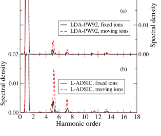
Figure 3: Harmonic generation in benzene during interaction with a 10-cycle circularly-polarised laser pulse having a peak intensity $I=$ $3.5\times 10^{14}\mbox{ W/cm}^{2}$ and wavelength $\lambda=$ 800 nm. We compare how the response changes when the ions are kept fixed and allowed to move. Plot (a) shows the calculation made using the LDA-PW92 exchange-correlation functional and plot (b) shows the calculation made using the L-ADSIC exchange-correlation functional.

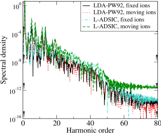
Figure 4: Harmonic generation in benzene during interaction with a 10-cycle circularly-polarised laser pulse having a peak intensity $I=$ $3.5\times 10^{14}\mbox{ W/cm}^{2}$ and wavelength $\lambda=$ 800 nm. Logarithmic plots of the four spectra in Fig. 3 are presented here. We can clearly see the formation of a plateau region. Based on the classical cut-off formula, the maximum plateau harmonic for this laser intensity and wavelength would be harmonic 49. We can clearly see that the intensities of the plateau harmonics increase when the L-ADSIC functional is used. In addition, for each functional, we see that the harmonic intensities are greater when the ions are allowed to move.

In order to study how the electrons and ions respond to the laser pulse, we can consider the response of the atom trajectories and the depletion of the Kohn-Sham orbitals (a measure of the amount of ionization). Fig. 5 presents the orbital response for the L-ADSIC calculations for benzene interacting with 10-cycle laser pulse of wavelength $\lambda=$ 800 nm and peak intensity $I=$ $3.5\times 10^{14}\mbox{ W/cm}^{2}$. Fig. 5(a) presents the results for fixed ions while Fig. 5(b) presents the results for moving ions. The reduction in orbital occupation gives a measure of the amount of ionization. For clarity, in these plots we only label the doubly-degenerate HOMO orbital [HOMO(a) and HOMO(b)]. In the case of fixed ions, we see that the HOMO orbital has the greatest response. However, we see that the other more tightly bound orbitals also respond significantly to the field. Hence, multielectron effects are important in describing the response of the molecule. When the ions are allowed to move the response is different. We now see that the total depletion is slightly greater, i.e. more ionization has occurred. Additionally, the response of the orbitals is also different. In this case some of the more tightly bound orbitals have a response similar to the HOMO orbitals. Again this shows that the ionic motion greatly alters the response of the molecule.

Polarisation	Intensity	Ions	Approximation	Harmonic Ratios
	($\times 10^{14}$W/cm2)			5/7	7/11	5/3	11/9	7/9	11/13
Circular	3.5	Fixed	LDA-PW92	3.2	0.9	11.0	6.8	6.1	—
Circular	3.5	Fixed	LDA-PW92	2.975	5.246	—	—	—	0.346
Circular	3.5	Moving	LDA-PW92	3.085	4.206	—	—	—	0.505
Circular	3.5	Fixed	L-ADSIC	2.768	2.603	—	—	—	1.184
Circular	3.5	Moving	L-ADSIC	3.149	7.660	—	—	—	0.537
Linear $\parallel$	3.5	Moving	L-ADSIC	1.304	1.486	4.546	1.111	1.650	5.312
Linear $\perp$	3.5	Moving	L-ADSIC	2.842	0.193	0.333	0.374	0.072	0.315
Linear	10.0	Experiment	—	—	1.25	—	0.50	0.50	—

Table 2: Ratios of harmonic intensities for a range of calculations using different approximations to the exchange-correlation functional and different descriptions of the ionic motion. For all calculations the interaction of benzene with a 10-cycle laser pulse having wavelength $\lambda=$ 800 nm and intensity $I=$ $3.5\times 10^{14}\mbox{ W/cm}^{2}$ was studied. Blank entries denote situations in which one of the harmonic intensities was too small to be reliably estimated. Our results are compared with the previous calculations of Baer et al Baer et al. (2003). For linear polarisation, we present the ratios of the given harmonics for two orientations of the molecule with the pulse. In the parallel case, the molecule lies in the $x-y$ plane with the pulse polarised in the $x$ direction. In the perpendicular case, the molecule lies in the $y-z$ plane with the pulse polarised in the $x$ direction. We compare the harmonic ratios with those measured experimentally by Hay et al Hay et al. (2000).

In Fig. 6 we plot the trajectories of the ions during the interaction with two different laser pulses. In Fig. 6(a) we consider the interaction of benzene with the 10-cycle laser pulse of wavelength $\lambda=$ 800 nm and peak intensity $I=$ $3.5\times 10^{14}\mbox{ W/cm}^{2}$. In this case we see significant response of the ions to the laser, even over this 26 fs timeframe. As expected, this response is greatest for the hydrogen atoms, which are observed to spiral around in the field. The increase in the ionic displacement during the interaction clearly increases the probability for recollisions to occur. In Fig. 6(b) we consider a calculation in which the peak laser intensity has been lowered to $I=$ $2.0\times 10^{14}\mbox{ W/cm}^{2}$, i.e. the same as that used in Fig. 2(b). In this case we see that while the hydrogen ions respond to the field, the overall response is much less than that observed at the higher intensity. Additionally, the hydrogen ions now respond more randomly to the field. This can be understood in terms of the laser potential dominating the Coulomb potential at the higher intensity. At the lower intensity collective modes of motion will be present and so the trajectory of individual atoms may appear more random.

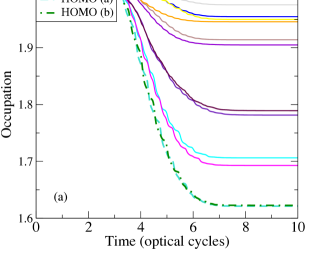
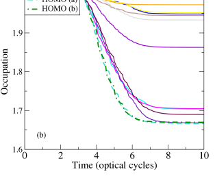
Figure 5: Populations of the Kohn-Sham orbitals of benzene during the interaction with a 10-cycle circularly-polarised laser pulse of wavelength $\lambda=$ 800 nm and intensity $I=$ $3.5\times 10^{14}\mbox{ W/cm}^{2}$. In (a) the ions are kept fixed during the simulation while in (b) the ions are allowed to move. All calculations were performed using the L-ADSIC exchange-correlation functional. In the simulations both the molecule and the polarisation of the laser lie in the $x-y$ plane. For clarity we only label the two forms of the doubly degenerate HOMO orbital: these are referred to as HOMO(a) and HOMO(b). The reduction of the population due to the wavefunction splitting method provides a measure of the amount of ionization. By the end of the pulse the total electron depletion is 2.06 for the moving ion calculation, compared to 1.98 for the fixed-ion calculation.

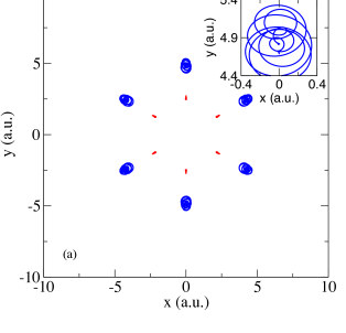
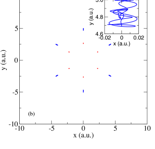
Figure 6: Ion trajectories for benzene during the interaction with a 10-cycle circularly-polarised laser pulse of wavelength $\lambda=$ 800 nm. In (a) the peak laser intensity is $I=$ $3.5\times 10^{14}\mbox{ W/cm}^{2}$ while in (b) it is $I=$ $2.0\times 10^{14}\mbox{ W/cm}^{2}$. All calculations were performed using the L-ADSIC exchange-correlation functional. Red trajectories correspond to carbon atoms while blue trajectories correspond to hydrogen ions. For clarity, the inset figures show the trajectory of the top hydrogen atom in the $x-y$ plane.

III.2 Molecular response to linearly-polarised light

At this point we have shown that the ionic motion plays a crucial role in the dynamical response of benzene to circularly-polarised light. We would now like to investigate how the molecule responds to linearly-polarised light. In Fig. 2(a) we have already shown a snapshot of the electronic density for benzene interacting with a 10-cycle linearly-polarised laser pulse of wavelength $\lambda=$ 800nm and peak intensity $I=$ $2.0\times 10^{14}\mbox{ W/cm}^{2}$. In that case the laser field was aligned in the $x$ direction, i.e. in the plane of the molecule. In Fig. 7 we show the harmonic spectra whenever the laser intensity increases to $I=$ $3.5\times 10^{14}\mbox{ W/cm}^{2}$. Two orientations of the molecule are considered. In the parallel orientation the molecule lies in the $x-y$ plane with the laser aligned along $x$. In the perpendicular orientation the molecule lies in the $y-z$ plane with the laser aligned along $x$. In both simulations the L-ADSIC approximation to the exchange-correlation functional is used and the ions are allowed to move. We plot the spectra along the laser polarisation direction, i.e. $S_{x}(\omega)$. We see that the spectra obtained are quite different to those obtained using circularly-polarised pulses. In particular, for linear polarisation the plateau regions are more pronounced (the cut-off harmonics in this case agree well with that predicted by the cut-off formula Corkum (1993); Kulander et al. (1993)). Comparing the two sets of results in Fig. 7, we see that the harmonics produced in the parallel orientation are largest for low-order harmonics while the plateau harmonics are greatest in the perpendicular orientation. This is in agreement with our previous LDA calculations that considered fixed ions Dundas (2012).

For the lowest harmonics we can calculate their relative strengths. These are presented at the end of Table 2. We see that the ratios of these harmonics vary dramatically when the molecule-laser orientation is changed. In the table, we also show experimental ratios from Hay et al Hay et al. (2000). While these experimental results were obtained for a larger laser intensity, we see that our ratios are in broad agreement. It is also clear from the results in this table that there is a large difference between the ratios obtained for linear and circular polarisation. This clearly illustrates the different mechanisms and selection rules that apply in each case.

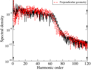
Figure 7: Calculated harmonic spectra for benzene interacting with a 10-cycle linearly polarised laser pulse having wavelength $\lambda=$ 800 nm and peak intensity $I=$ $3.5\times 10^{14}\mbox{ W/cm}^{2}$. For both simulations the L-ADSIC functional was used and the ions were allowed to move. Results for two orientations of the molecule with the pulse are considered. In the parallel case, the molecule lies in the $x-y$ plane with the pulse polarised in the $x$ direction. In the perpendicular case, the molecule lies in the $y-z$ plane with the pulse polarised in the $x$ direction.

We can obtain more information about the molecular response by looking at the Kohn-Sham orbital populations and the trajectories of the ions. Fig. 8 presents the populations of the Kohn-Sham orbitals for each calculation considered in Fig. 7 together with the ion trajectories. From the ion trajectories we see that the ionic displacements are similar for both orientations considered. However, the response of the Kohn-Sham orbitals is markedly different. In the parallel case shown in Fig. 8(c) we see that the HOMO(a) and HOMO(b) orbitals respond differently to the field and that several of the more tightly bound orbitals respond more strongly to the pulse than the HOMO(b) orbital. In the perpendicular orientation we see that both HOMO orbitals respond almost identically and their response is much greater than the more tightly bound orbitals. This behaviour is similar to that observed in our earlier fixed-ion calculations using the LDA functional Dundas (2012).

We now consider the difference in the response of benzene to linearly- and circularly-polarised laser pulses. A number of experiments have previous considered this difference Talepour et al. (2000); Rajgara et al. (2003). In the results of Talepour et al Talepour et al. (2000) it was shown that for a laser intensity of $I=$ $6.0\times 10^{14}\mbox{ W/cm}^{2}$ the fragmentation patterns observed were largely independent of the laser polarisation. Later, experiments by Rajara et al Rajgara et al. (2003) showed that for a higher laser intensity of $I=$ $1.0\times 10^{16}\mbox{ W/cm}^{2}$ the fragment yields were much greater for linear polarisation. They explained this difference as due to electron recollisions in circularly-polarised pulses being more probable at lower laser intensities. While our results cannot be directly compared with experiment since important propagation effects are not taken into account Jin et al. (2011b); Zhao et al. (2011); Jin et al. (2012), our results support these observations. Comparing Fig. 5(b) with Fig. 8(c), we see that the population loss from the Kohn-Sham orbitals is greatest during interaction with the linearly-polarised pulse. Additionally, comparing Fig. 6(a) with Fig. 8(a) we see that the ionic response is slightly greater for both linear polarisation. Lastly, referring to Fig. 2 again, we see clear evidence of recollision for circular polarisation.

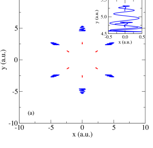
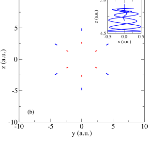
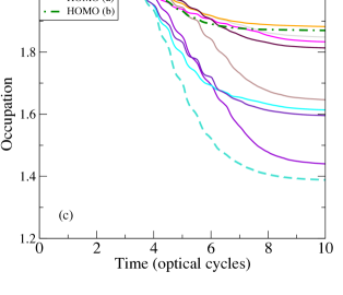
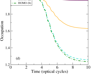
Figure 8: Populations of the Kohn-Sham orbitals and ion trajectories for benzene during the interaction with a 10-cycle linearly-polarised laser pulse of wavelength $\lambda=$ 800 nm and peak intensity $I=$ $3.5\times 10^{14}\mbox{ W/cm}^{2}$. (a) and (c) respectively present the trajectories and populations for the parallel orientation between the molecule and the field while (b) and (d) respectively present the trajectories and populations for the perpendicular orientation. For both simulations the L-ADSIC functional was used. In the trajectory plots, red corresponds to carbon atoms while blue corresponds to hydrogen ions. In the population plots we only label the two forms of the doubly degenerate HOMO orbital [HOMO(a) and HOMO(b)] for clarity. In all cases the laser polarisation direction is aligned along the $x$ axis. The main plot of (b) presents the trajectories in the plane of the molecule (the $y-z$ plane). To show the response along the laser polarisation axis, the inset shows the trajectory of the top hydrogen atom in the $x-z$ plane. The inset in plot (a) shows the extent of the same hydrogen atom in the parallel orientation.

IV Conclusions

In this paper we have studied harmonic generation in benzene using a TDDFT approach in which the ions were allowed to move classically while the exchange-correlation functional included self-interaction corrections. The response to both linearly- and circularly-polarised IR laser pulses having durations of $\sim$ 26 fs was considered. For all calculations we find that the ionic motion has a large effect on the harmonic response, even for such short duration pulses. In addition, we find that the displacement of the ions is slightly greater when linearly-polarised light is used. Even though the probability of electron recollision in circularly-polarised pulses is lower, we still see evidence of recollisions in the harmonic spectra. We find that plateau harmonics (especially in the secondary plateau) are enhanced when the ions are allowed to move. We believe this is due to electrons that ionize from one ionic centre recolliding with a different ionic centre. When the ions are allowed to move the increased ionic response gives a greater probability for these recollisions to occur.

Baer et al Baer et al. (2003) observed a secondary plateau in their calculations for benzene aligned in the plane of a circularly-polarised pulse and predicted that the length of this plateau would be similar or longer than the plateau obtained for non-aligned benzene interacting with linearly-polarised pulses. In our calculations we have found that this is the case. However, we also find that the intensity of the plateau harmonics increases when the ions are allowed to move. Additionally we find that the population depletion from the Kohn-Sham orbitals is only slightly greater for linearly-polarised pulses than for circularly-polarised pulses, in agreement with experimental observations at similar intensities.

The method we have used is robust enough to describe general polyatomic molecules interacting with laser pulses of arbitrary polarisation. We can consider laser wavelengths ranging from vacuum ultraviolet (VUV) to IR. This opens up the possibility of carrying out simulations with attosecond pulses having both circular and linear polarisation. Therefore, we have a tool for studying circular dichroism in chiral molecules using HHG.

V Acknowledgements

This work used the ARCHER UK National Supercomputing Service (http://www.archer.ac.uk) and has been supported by COST Action CM1204 (XLIC). AW acknowledges financial support through a PhD studentship funded by the UK Engineering and Physical Sciences Research Council.

References

- Bandrauk et al. (2007) A. D. Bandrauk, S. Barmaki, S. Chelkowski, and G. Lafmago Kamta, in Progress in Ultrafast Laser Science Volume III, edited by K. Yamanouchi (Kluwer, Amsterdam, 2007) p. 1.
- Ferré et al. (2015) A. Ferré, C. Handschin, M. Dumergue, F. Burgy, A. Comby, D. Descamps, B. Fabre, G. A. Garcia, R. Géneaux, L. Merceron, E. Mével, L. Nahon, S. Petit, B. Pons, D. Staedter, S. Weber, T. Ruchon, V. Blanchet, and Y. Mairesse, Nature Photonics 9, 93 (2015).
- Wong et al. (2011) M. C. H. Wong, J.-P. Brichta, M. Spanner, S. Patchkovskii, and V. R. Bhardwaj, Phys. Rev. A 84, 051403(R) (2011).
- Cireasa et al. (2015) R. Cireasa, A. E. Boguslavskiy, B. Pons, M. C. H. Wong, D. Descamps, S. Petit, H. Ruf, N. Thiré, A. Ferré, J. Suarez, J. Higuet, B. E. Schmidt, A. F. Alharbi, F. Légaré, V. Blanchet, B. Fabre, S. Patchkovskii, O. Smirnova, Y. Mairesse, and V. R. Bhardwaj, Nature Physics 11, 654 (2015).
- Remacle and Levine (2006) F. Remacle and R. D. Levine, Proc Nat Acad Sci 103, 6793 (2006).
- Krausz and Ivanov (2009) F. Krausz and M. Ivanov, Rev. Mod. Phys. 81, 163 (2009).
- Corkum (1993) P. B. Corkum, Phys. Rev. Lett. 71, 1994 (1993).
- Kulander et al. (1993) K. C. Kulander, K. J. Schafer, and J. L. Krause, in Super-Intense Laser-Atom Physics, edited by B. Piraux, A. L’Huillier, and K. Rzazewski (Plenum, New York, 1993) p. 95.
- Rajgara et al. (2003) F. A. Rajgara, M. Krishnamurthy, and D. Mathur, Phys. Rev. A 68, 023407 (2003).
- Mauger et al. (2010) F. Mauger, C. Chandre, and T. Uzer, Phys. Rev. Lett. 105, 083002 (2010).
- Alon et al. (1998) O. E. Alon, V. Averbukh, and N. Moiseyev, Phys. Rev. Lett. 80, 3743 (1998).
- Averbukh et al. (2001) V. Averbukh, O. E. Alon, and N. Moiseyev, Phys. Rev. A 64, 033411 (2001).
- Baer et al. (2003) R. Baer, D. Neuhauser, P. R. Žďánská, and N. Moiseyev, Phys. Rev. A 68, 043406 (2003).
- Runge and Gross (1984) E. Runge and E. K. U. Gross, Phys. Rev. Lett. 52, 997 (1984).
- He et al. (2008) F. He, A. Becker, and U. Thumm, Phys. Rev. Lett. 101, 213002 (2008).
- Kono et al. (1997) H. Kono, Y. O. A. Kita, and Y. Fujimura, J. Comp. Phys. 130, 148 (1997).
- Lein et al. (2003) M. Lein, P. P. Corso, J. P. Marangos, and P. L. Knight, Phys. Rev. A 67, 023819 (2003).
- Dundas et al. (2003) D. Dundas, K. J. Meharg, J. F. McCann, and K. T. Taylor, Euro. Phys. J. D 26, 51 (2003).
- Bandrauk and Lu (2004) A. D. Bandrauk and H. Lu, Int. J. Quant. Chem 99, 431 (2004).
- Vanne and Saenz (2010) Y. V. Vanne and A. Saenz, Phys. Rev. A 82, 011403(R) (2010).
- Kjeldsen et al. (2006) T. K. Kjeldsen, L. B. Madsen, and J. P. Hansen, Phys. Rev. A 74, 035402 (2006).
- Morales et al. (2014) F. Morales, P. Rivière, M. Richter, A. Gubaydullin, M. Ivanov, O. Smirnova, and F. Martin, J. Phys. B: At. Mol. Phys. 47, 204015 (2014).
- Hou et al. (2012) X.-F. Hou, L.-Y. Png, Q.-C. Ning, and Q. Gong, J. Phys. B: At. Mol. Phys. 45, 074019 (2012).
- Yuan and Bandrauk (2012) K.-J. Yuan and A. D. Bandrauk, Phys. Rev. A 85, 053419 (2012).
- Spanner and Patchkovskii (2009) M. Spanner and S. Patchkovskii, Phys. Rev. A 80, 063411 (2009).
- Smirnova et al. (2009) O. Smirnova, Y. M. S. Patchkovskii, N. Dudovich, D. Villeneuve, P. Corkum, and M. Y. Ivanov, Nature 460, 972 (2009).
- Chu and Chu (2004) X. Chu and S.-I. Chu, Phys. Rev. A 70, 061402 (2004).
- Dundas and Rost (2005) D. Dundas and J. M. Rost, Phys. Rev. A 71, 013421 (2005).
- Fowe and Bandrauk (2011) E. P. Fowe and A. D. Bandrauk, Phys. Rev. A 84, 035402 (2011).
- Petretti et al. (2010) S. Petretti, Y. V. Vanne, A. Saenz, A. Castro, and P. Decleva, Phys. Rev. Lett. 104, 223001 (2010).
- Le et al. (2009) A.-T. Le, R. R. Lucchese, S. Tonzani, T. Morishita, and C. D. Lin, Phys. Rev. A 80, 013401 (2009).
- Lin et al. (2010) C. D. Lin, A.-T. Le, T. Morishita, and R. R. Lucchese, J. Phys. B: At. Mol. Phys. 43, 122001 (2010).
- Jin et al. (2011a) C. Jin, A.-T. Le, and C. D. Lin, Phys. Rev. A 83, 053409 (2011a).
- Wong et al. (2013) M. C. H. Wong, A.-T. Le, A. F. Alharbi, A. E. Boguslavskiy, R. R. Lucchese, J.-P. Brichta, C. D. Lin, and V. R. Bhardwaj, Phys. Rev. Lett. 110, 033006 (2013).
- Le et al. (2013a) A.-T. Le, R. R. Lucchese, and C. D. Lin, Phys. Rev. A 87, 063406 (2013a).
- Le et al. (2013b) A.-T. Le, R. R. Lucchese, and C. D. Lin, Phys. Rev. A 88, 021402(R) (2013b).
- Telnov and Chu (2009) D. A. Telnov and S.-I. Chu, Phys. Rev. A 80, 043412 (2009).
- Heslar et al. (2011) J. Heslar, D. Telnov, and S.-I. Chu, Phys. Rev. A 83, 043414 (2011).
- Kunert and Schmidt (2003) T. Kunert and R. Schmidt, Euro. Phys. J. D 25, 15 (2003).
- Uhlmann et al. (2003) M. Uhlmann, T. Kunert, F. Grossmann, and R. Schmidt, Phys. Rev. A 67, 013413 (2003).
- Dundas (2004) D. Dundas, J. Phys. B: At. Mol. Opt. Phys. 37, 2883 (2004).
- Calvayrac et al. (2000) F. Calvayrac, P.-G. Reinhard, E. Suraud, and C. A. Ullrich, Phys Rep 337, 493 (2000).
- Castro et al. (2004) A. Castro, M. A. L. Marques, J. A. Alonso, G. F. Bertsch, and A. Rubio, Eur. Phys. J. D 28, 211 (2004).
- Dundas (2012) D. Dundas, J. Chem. Phys. 136, 194303 (2012).
- Wopperer et al. (2012) P. Wopperer, P. M. Dinh, E. Suraud, and P.-G. Reinhard, Phys. Rev. A 85, 015402 (2012).
- Crawford-Uranga et al. (2014) A. Crawford-Uranga, U. D. Giovannini, D. J. Mowbray, S. Kurth, and A. Rubio, J. Phys. B: At. Mol. Phys. 47, 124018 (2014).
- Troullier and Martins (1991) N. Troullier and J. L. Martins, Phys. Rev. B 43, 1993 (1991).
- Kleinman and Bylander (1982) L. Kleinman and D. M. Bylander, Phys. Rev. Lett. 48, 1425 (1982).
- Oliveira et al (2008) M. J. T. Oliveira et al, Computer Physics Communications 178, 524 (2008).
- Meijer and Sprik (1996) E. J. Meijer and M. Sprik, J. Chem. Phys. 105, 8684 (1996).
- Sharifi et al. (2007) S. M. Sharifi, A. Talebpour, and S. L. Chin, J. Phys. B: At. Mol. Phys. 40, F259 (2007).
- Perdew and Wang (1992) J. P. Perdew and Y. Wang, Phys. Rev. B 45, 13244 (1992).
- Legrand et al (2002) C. Legrand et al, J. Phys. B: At. Mol. Opt Phys 35, 1115 (2002).
- Arnoldi (1951) W. E. Arnoldi, Q. Appl. Math 9, 17 (1951).
- Smyth et al (1998) E. S. Smyth et al, Computer Physics Communications 114, 1 (1998).
- Ullrich (2000) C. A. Ullrich, J. Mol. Struc. - Theochem 501, 315 (2000).
- National Institute of Standards and Technology Chemistry WebBook() (NIST) National Institute of Standards and Technology (NIST) Chemistry WebBook, http://webbook.nist.gov/chemistry.
- Burnett et al. (1992) K. Burnett, V. C. Reed, J. Cooper, and P. L. Knight, Phys. Rev. A 45, 3347 (1992).
- Hay et al. (2000) N. Hay, R. de Nalda, T. Halfmann, K. J. Mendham, M. B. Mason, M. Castillejo, and J. P. Marangos, Phys. Rev. A 62, 041803 (2000).
- Talepour et al. (2000) A. Talepour, A. D. Bandrauk, K. Vijayalakshmi, and S. L. Chin, J. Phys. B: At. Mol. Phys. 33, 4615 (2000).
- Jin et al. (2011b) C. Jin, H. J. Wörner, V. Tosa, A.-T. Le, J. B. Bertrand, R. R. Lucchese, P. B. Corkum, D. M. Villeneive, and C. D. Lin, J. Phys. B: At. Mol. Phys. 44, 095601 (2011b).
- Zhao et al. (2011) S.-F. Zhao, C. Jin, R. R. Lucchese, A.-T. Le, and C. D. Lin, Phys. Rev. A 83, 033409 (2011).
- Jin et al. (2012) C. Jin, J. B. Bertrand, R. R. Lucchese, H. J. Wörner, P. B. Corkum, D. M. Villeneive, A.-T. Le, and C. D. Lin, Phys. Rev. A 85, 013405 (2012).