Estimates of $Z^{\prime}$ couplings within data on the $A_{FB}$
for Drell-Yan process at the LHC at $\sqrt{s}=7$ and $8$ TeV

Abstract

Model-independent search for the Abelian $Z^{\prime}$ gauge boson in the Drell-Yan process at the LHC at $\sqrt{s}=7$  and 8 TeV is fulfilled. Estimations of the $Z^{\prime}$ axial-vector coupling $a_{f}^{2}$ to the Standard model fermions, the couplings of the axial-vector to lepton vector currents $a_{f}v_{l}$ and the couplings of the axial-vector to quark vector currents $a_{f}v_{q}$ are derived within data on the forward-backward asymmetry presented by the CMS Collaboration. The analysis takes into consideration the behaviour of the differential cross-section which exhibits itself if the derived already special relations between the couplings proper to the renormalizable theories are accounted for. In particular, they hold in all the models of Abelian $Z^{\prime}$ usually considered in the model-dependent analysis of the LHC data. The coupling values are estimated at $\sim$92 % CL by means of the maximum likelihood function. They weakly depend on the $Z^{\prime}$ mass in the investigated interval 1.2 TeV $<m_{Z^{\prime}}<$ 5 TeV. Taking into account the dependence of $Z-Z^{\prime}$ mixing angle $\theta_{0}$ on $m_{Z^{\prime}}$ and the LEP constraints $|\theta_{0}|\sim 10^{-3}-10^{-4}$, the optimistic limits on $m_{Z^{\prime}}$ are established as $3<m_{Z^{\prime}}<7-8$ TeV. Comparison with the results of other authors is given.

I Introduction

After discovery of the Higgs boson at the LHC, the Standard model (SM) is considered to be completed. From ”practical” computational point of view it means that the neutral scalar particle of the mass 125 GeV has to be taken into consideration for all the processes investigated. If we also believe that the spontaneous symmetry breaking mechanism is operating to supply particle masses, the Higgs particle has to be considered as a fundamental point like state belonging to a renormalizable theory. This also concerns new models extending the SM at high energies and containing various scalar particles.

Searching for new physics is the main goal of experiments at the LHC. One of expected heavy particles is an Abelian $Z^{\prime}$ gauge boson predicted by numerous extended models (see review papers A. Leike (1999) – Accomando, Elena and Belyaev, Alexander and Fedeli, Luca and King, Stephen F. and Shepherd-Themistocleous, Claire (2011)). It is introduced as the field related with an additional $\tilde{U}(1)$ group to the SM gauge group. Lower bounds for its mass have been obtained at the LEP (J. Alcaraz, P. Azzurri, A. Bajo-Vaquero et al. (2007), The OPAL Collaboration, G. Abbiendi et al. (2004), The DELPHI Collaboration, J. Abdallah et al. (2006)), Tevatron A. Ferroglia, A. Lorca, J.J. van der Bij (2007) and first run LHC experiments Accomando, Elena and Belyaev, Alexander and Fedeli, Luca and King, Stephen F. and Shepherd-Themistocleous, Claire (2011) in either model-dependent or model-independent approaches. The present day model-dependent published lower bound on the mass is $m_{Z^{\prime}}>2.5$ TeV from the CMS results and $m_{Z^{\prime}}>2.9$ TeV from the ATLAS ones. At present about hundred $Z^{\prime}$ models are discussed in the literature. In model-dependent searches established, only the most popular ones such as $LR$, $ALR$, $\chi$, $\psi$, $\eta$, B - L, $SSM,$ have been investigated and the particle mass is estimated. These models are also used as benchmarks in introducing the efficient observables for future experiments at the ILC P. Osland, A. A. Pankov and A. V. Tsytrinov (2010), T. Han, P. Langacker, Z. Liu and L.-T. Wang (2013). In this approach, the couplings to the SM particles were fixed as in the specific considered models and therefore not estimated. As it also occurred, the identification reach for different models is about the estimated $m_{Z^{\prime}}$ lower masses. So that it is problematic to distinguish the basic $Z^{\prime}$ model at the LHC. In such a situation, model-independent approaches are also very perspective. They give a possibility for estimating not only the particle mass but also some $Z^{\prime}$ couplings to the SM fermions. Hence, definite classes of the extended models could be restricted.

In studies of perspective variables for identification of the $Z^{\prime}$ models T. Han, P. Langacker, Z. Liu and L.-T. Wang (2013), in particular, it was concluded that, as complementary way, a model-independent approach is very desirable. Estimations of couplings can be further used in specifying the basic $Z^{\prime}$ model. Usually, the couplings are considered as independent arbitrary numbers. However, this is not the case and they are correlated parameters, if some natural requirements, which this model has to satisfy, are assumed. In most cases we believe that the basic model is renormalizable one. Hence, correlations follow and the amount of free parameters reduces. Moreover, the correlations between couplings influence kinematics of the processes that gives a possibility for introducing the specific observables which uniquely pick out the virtual state of interest – $Z^{\prime}$ boson in our case. The noted additional requirement assumes searching for new particles within the class of renormalizable models. In other aspects the models are not specified. Below, we say ”model-independent approach” for the analysis when either the mass or the couplings must be fitted. Such type approach is in-between the usual model-dependent method, when all the couplings are fixed and only the mass $m_{Z^{\prime}}$ is free parameter, and model-independent searches assuming complete independence of couplings describing new physics. Recent review on searching for the Abelian $Z^{\prime}$ boson in the model-independent approach is Gulov and Skalozub (2010)

In what follows, we search for the Abelian $Z^{\prime}$ boson belonging to a renormalizable model. We also assume that there is only one additional heavy particle relevant at considered energies. There are numerous models of such type. In particular, most of $E_{6}$ motivated models and mentioned above ones enter this class. The used in the present analysis relations 5 are proper to this class. In particular, they hold in the models noted above. These relations have been derived already in two ways A. V. Gulov, V. V. Skalozub (2001), A. V. Gulov, V. V. Skalozub (2000). For convenience of readers, we adduce more details about them in Appendix B. In what follows, we say $Z^{\prime}$ boson for the Abelian one, only. We also assume that the SM is the subgroup of the extended group and therefore no interactions of the type $~{}ZZ^{\prime}W^{+}W^{-}$ appear in the tree-level Lagrangian.

In the present paper, we search for the $Z^{\prime}$ at the LHC on the base of the CMS data on the forward-backward asymmetry, $A_{FB}$, for the Drell-Yan annihilation process measured at energy $\sqrt{s}=7$ TeV The CMS Collaboration (2013) and 8 TeV The CMS Collaboration (2016a). As we show below, this observable is fine sensitive to the $Z^{\prime}$ signals due to kinematics properties of the differential cross-sections of the process. The advantage of the Drell-Yan process is that it is a ”pure” one and we do not need to take the hadronization effects into consideration. We suppose that in this process the $Z^{\prime}$ manifests itself as the intermediate state like the $Z$ boson and the photon. But it is a heavy particle and all the loops of it are decoupled at investigated energies. As a result, the $Z^{\prime}$ exhibits itself as the special kind external field. It modifies the observables as compared to the SM predictions. In paper The CMS Collaboration (2013) presented by the CMS collaboration it is noted that all the measured $A_{FB}$ values are in agreement with the SM expectations at $1-2\sigma$ confidence level (CL). So that there is no indication of new physics. However, in that data there is a significant number of points closely located to the CL area boundary. So that it is of interest to verify whether the data on $A_{FB}$ could result in signals (hints, in fact) for new heavy particle – the Abelian $Z^{\prime}$ gauge boson.

The $A_{FB}$ of the Drell-Yan lepton-antilepton pair is chosen as the observable for the experimental data processing. Reasons for this are discussed in the next section. This quantity turns out to be very sensitive to small changes of used parameters. Also, its theoretical uncertainty, which originates from the PDF uncertainty, is much smaller than the one of the total cross-sections. Thus, the $A_{FB}$ yields quite precise results for measured quantities. Also, in recent paper The CMS Collaboration (2015) it was motivated the complementarity of the $A_{FB}$ to the total cross-section in searching for the $Z^{\prime}$ as resonance state. Our model-independent analysis supports this idea for lower beam energies. In fact, within huge amount of data accumulated at the LHC at different energies one is able to estimate various important parameters which could be used in further studies.

As we show, the CMS data on the $A_{FB}$ admit the $Z^{\prime}$ existence. By using the maximum likelihood function method we estimate the $Z^{\prime}$ couplings to the SM fermions for the $Z^{\prime}$ mass in the interval 1.2 TeV $<m_{Z^{\prime}}<5$ TeV and obtain that these couplings are to be non-zero with the 92 % CL accuracy. Taking into account the estimated value of $a^{2}_{f}$ and experimental upper bound on mixing angle $|\theta_{0}|\sim 10^{-3}-10^{-4}$ Jens Erler, Paul Langacker, Shoaib Munir and Eduardo Rojas (2009) the estimates of the mass $3<m_{Z^{\prime}}<7-8$ TeV are derived.

The paper is organized as follows. In the next section we present the cross-sections of the process investigated and its angular distributions at various values of the effective mass for lepton pairs. The observed behaviour of different factor functions entering the cross-section gives reasons for introducing the $A_{FB}$ as convenient observable. In section 3 the estimations of the couplings are carried out. Section 4 is devoted to discussion and comparison with the results of other authors. In Appendix A, we present the behaviour of the $F_{k}$ factors entering Eq. 13. Appendix B contains necessary information about the equations 4, 5. Appendix C includes detailed information about the PDF uncertanties.

II Cross-section with the $Z^{\prime}$

In this section, we calculate the cross-section of the Drell-Yan process in the model-independent approach and obtain its dependence on the $Z^{\prime}$ couplings.

We start with the differential cross-section in the parton model written in the Collins-Soper frame J. Collins (1977):

$$\frac{d^{3}\sigma}{dM\,dY\,dz}=\sum_{q}{M\left[\mathrm{xf}_{q}\left(\frac{M}{\sqrt{s}}e^{Y}\right)\mathrm{xf}_{\bar{q}}\left(\frac{M}{\sqrt{s}}e^{-Y}\right)\frac{d\hat{\sigma}_{q}(z)}{dz}\right.}+\left.\mathrm{xf}_{q}\left(\frac{M}{\sqrt{s}}e^{-Y}\right)\mathrm{xf}_{\bar{q}}\left(\frac{M}{\sqrt{s}}e^{Y}\right)\frac{d\hat{\sigma}_{q}(-z)}{dz}\right].$$ (1)

Here, $\hat{\sigma}$ is the parton-level cross-section: $\hat{\sigma}_{q}\equiv\sigma_{q\bar{q}\to l^{+}l^{-}}$ and $l^{+}l^{-}$ are final lepton states. Everywhere below we denote the parton-level quantities with the hatted letters and the appropriated hadron-level quantities, which are already integrated with PDFs, with the non-hatted ones. $M$ is dilepton invariant mass, $Y$ is an intermediate state rapidity, $z=\cos\theta_{CS}$, where $\theta_{CS}$ is a dilepton scattering angle. We take into account the known relations between the quark $x_{1}$ and antiquark $x_{2}$ momentum fractions: $x_{1,2}=(M/\sqrt{s})e^{\pm Y}$. The functions $f_{q}(x)$ are the PDF distributions, and the functions $\mathrm{xf}_{q}(x)=xf_{q}(x)$ are pre-implemented in the majority of PDF computer packages. In 1 we sum over the quarks only, not over both the quarks and antiquarks.

To proceed we have to calculate the parton-level cross-section $\hat{\sigma}_{q\bar{q}\to l^{+}l^{-}}$ taking into account the $Z^{\prime}$ contributions. The effective low energy Lagrangian describing the interaction of the heavy $Z^{\prime}$ with the SM particles was introduced in G. Degrassi and A. Sirlin (1989), M. Cvetic and B. W. Lynn (1987). Its part related to our problem and describing interactions between the fermions and the $Z$ and $Z^{\prime}$ mass eigenstates reads (see, for example, Gulov and Skalozub (2010)):

$$\begin{split}{\mathcal{L}}_{Z\bar{f}f}=\frac{1}{2}Z_{\mu}\bar{f}\gamma^{\mu}[(v^{\mathrm{SM}}_{fZ}+\gamma^{5}a^{\mathrm{SM}}_{fZ})\cos\theta_{0}\\ +(v_{f}+\gamma^{5}a_{f})\sin\theta_{0}]f,\end{split}$$ (2)

$$\begin{split}{\mathcal{L}}_{Z^{\prime}\bar{f}f}=\frac{1}{2}Z^{\prime}_{\mu}\bar{f}\gamma^{\mu}[(v_{f}+\gamma^{5}a_{f})\cos\theta_{0}\\ -(v^{\mathrm{SM}}_{fZ}+\gamma^{5}a^{\mathrm{SM}}_{fZ})\sin\theta_{0}]f,\end{split}$$ (3)

where $f$ is an arbitrary SM fermion state; $v^{\mathrm{SM}}_{fZ}$, $a^{\mathrm{SM}}_{fZ}$ are the SM axial-vector and vector couplings of the $Z$-boson, $a_{f}$ and $v_{f}$ are the ones for the $Z^{\prime}$, $\theta_{0}$ is the $Z$–$Z^{\prime}$ mixing angle. Within the considered formulation, this angle is determined by the coupling $\tilde{Y}_{\phi}$ of fermions to the scalar field as follows (see Gulov and Skalozub (2010) and Appendix B for details)

$$\theta_{0}=\frac{\tilde{g}\sin\theta_{W}\cos\theta_{W}}{\sqrt{4\pi\alpha_{\mathrm{em}}}}\frac{m^{2}_{Z}}{m^{2}_{Z^{\prime}}}\tilde{Y}_{\phi}+O\left(\frac{m^{4}_{Z}}{m^{4}_{Z^{\prime}}}\right),$$ (4)

where $\theta_{W}$ is the SM Weinberg angle, $\tilde{g}$ is $\tilde{U}(1)$ gauge coupling constant and $\alpha_{\mathrm{em}}$ is electromagnetic fine structure constant. Although the mixing angle is small quantity of order ($m^{2}_{Z}/m^{2}_{Z^{\prime}}$), it contributes to the $Z$-boson exchange amplitude and cannot be neglected.

As it was shown in Gulov and Skalozub (2010), A. V. Gulov, V. V. Skalozub (2001), A. V. Gulov, V. V. Skalozub (2000), if the extended model is renormalizable and contains the SM as a subgroup, the relations between the couplings hold:

$$v_{f}-a_{f}=v_{f^{*}}-a_{f^{*}},\quad a_{f}=T_{3f}\tilde{g}\tilde{Y}_{\phi}.$$ (5)

Here $f$ and $f^{*}$ are the partners of the $SU(2)_{L}$ fermion doublet ($l^{*}=\nu_{l},\nu^{*}=l,q^{*}_{u}=q_{d}$ and $q^{*}_{d}=q_{u}$), $T_{3f}$ is the third component of the weak isospin. These relations are proper for the models of Abelian $Z^{\prime}$. They are just as in the SM for proper values of the hypercharges $Y^{R}_{f},Y^{L}_{f},Y_{\phi}$ of the left-handed, right-handed fermions and scalars. The correlations can be derived from the necessary requirement of renormalizability that there are no new divergent structures appearing in one-loop order. The divergencies could appear at the structures presented in the initial tree-level Lagrangian, only. If these conditions do not hold, the theory is not renormalizable. But if they fulfil in one-loop order, there is no guarantee that this will be the case in higher orders or with accounting for of anomalies. The latter two questions are more delicate. They require detailed information about the particle content of the model. Thus, the correlations 5 are the necessary conditions for renormalizability. Other way of derivation 5 is presented in Appendix B.

The couplings of the $Z^{\prime}$ to the axial-vector fermion current have a universal absolute value proportional to the $Z^{\prime}$ coupling to the scalar doublet. Then, the $Z$–$Z^{\prime}$ mixing angle (4) can be determined by the axial-vector coupling. As a result, the number of independent parameters is significantly reduced. This universality follows due to exchange of the scalar particles. In particular, the relations 5 hold in Two-Higgs-Doublet SM (see Appendix B). Because of the universality, we will omit the subscript $f$ and write $a$ for axial-vector coupling. It is convenient for what follows to introduce the ”normalized” couplings

$$\bar{a}=\frac{1}{\sqrt{4\pi}}\frac{m_{Z}}{m_{Z^{\prime}}}~{}a,~{}~{}\bar{v}_{f}=\frac{1}{\sqrt{4\pi}}\frac{m_{Z}}{m_{Z^{\prime}}}~{}v_{f}.$$ (6)

As it follows from (2), (3), the Drell-Yan process cross-section has the contribution from the SM, the contribution from $Z-Z^{\prime}$ interference, and from the $Z^{\prime}$ part. The last contribution can be neglected at energies not close to a $Z^{\prime}$ resonance peak. Hence, taking into account (5), the parton-level cross-section can be written as

$$\begin{split}\frac{d\hat{\sigma_{q}}}{dz}=\left(\frac{d\hat{\sigma_{q}}}{dz}\right)_{SM}+\bar{a}^{2}\hat{F}_{q1}+\bar{a}\bar{v}_{l}\hat{F}_{q2}\\ +\bar{a}\bar{v}_{u}\hat{F}_{q3}+\bar{v}_{l}\bar{v}_{u}\hat{F}_{q4},\end{split}$$ (7)

where $\hat{F}_{qk}=\hat{F}_{qk}(M,z)$ are known from calculation kinematics factors, $q$ in the subscript is ”$u$” or ”$d$” (for up and down quarks, respectively), subscript ”l” denotes the $Z^{\prime}$ to lepton coupling, and subscript ”u” denotes the $Z^{\prime}$ to up-quark coupling. Thus, there are four unknown parameters which should be estimated from experiments. However, due to obvious relation $a^{2}\bar{v}_{l}\bar{v}_{u}=\bar{a}\bar{v}_{l}\bar{a}\bar{v}_{u}$ the parameter $\bar{v}_{l}\bar{v}_{u}$ can be expressed through three others. So, in general three-parameter fit is needed. Let us check whether it is possible to find an integral observable containing less amount of unknown parameters.

For doing that we consider the behaviour of the $\hat{F}_{qk}$ functions. In our analysis, these functions were calculated in an improved Born approximation in one-loop order. In the $Z-Z^{\prime}$ interference part, the loops with the SM particles coming from the $Z^{\prime}$ exchange part were computed analytically whereas the SM contributions have been calculated by using the PYTHIA package.

We investigate the behaviour of the hadron-level factors

$$F_{k}(M,Y,z)=\sum_{q}{M\left[\mathrm{xf}_{q}\left(\frac{M}{\sqrt{s}}e^{Y}\right)\mathrm{xf}_{\bar{q}}\left(\frac{M}{\sqrt{s}}e^{-Y}\right)\hat{F}_{k}(M,z)\right.}+\left.\mathrm{xf}_{q}\left(\frac{M}{\sqrt{s}}e^{-Y}\right)\mathrm{xf}_{\bar{q}}\left(\frac{M}{\sqrt{s}}e^{Y}\right)\hat{F}_{k}(M,-z)\right],$$ (8)

which are defined correspondingly to (1). The plots of the $F_{k}(M,Y,z)$ $z$-dependence at fixed $M$, $Y$ are shown in Figures A.1 – A.7 of Appendix A. For small invariant masses ($M<100-120$ GeV), the $F_{3}$ and $F_{4}$ functions are almost symmetric and therefore are suppressed in $A_{FB}$. This observation leads to idea that only the two first terms in (7) are dominant for the asymmetry. However, such behaviour does not preserve for more heavy $M$ bins ($M>100-120$ GeV). As we see in the figures A.5 – A.7, in this case the $F_{3}$ and $F_{4}$ functions demonstrate behaviour which significantly contribute to the asymmetry. So that the number of the unknown functions could not be reduced for heavy invariant masses. Nevertheless, the $A_{FB}$ remains convenient observable because it is very sensitive to the the small changes of the coupling values everywhere. Thus, to analyze the $A_{FB}$, we preserve in the cross-section $\frac{d^{3}\sigma}{dM\,dY\,dz}$ all the terms entering 7.

Next important notice is that the CMS detector has a finite acceptance and only the leptons with $p_{T}>p_{0}=20$ GeV can be detected. Therefore, to obtain the cross-section of interest we have to integrate the distributions over $z$ in the interval $-z_{0}$ to $+z_{0}$, where

$$z_{0}=\sqrt{1-4p^{2}_{0}/M^{2}}.$$ (9)

III Estimation of $Z^{\prime}$ couplings

The forward-backward asymmetry is defined as

$$A_{FB}=\frac{\sigma_{F}-\sigma_{B}}{\sigma_{F}+\sigma_{B}},$$ (10)

where

$$\sigma_{F}=\int_{0}^{z_{0}}\frac{d\sigma}{dz}dz,~{}~{}\sigma_{B}=\int_{-z_{0}}^{0}\frac{d\sigma}{dz}dz$$ (11)

and $z_{0}$ is given in (9). Providing the notations

$$\Delta=\sigma_{F}-\sigma_{B},~{}~{}\Sigma=\sigma_{F}+\sigma_{B},$$ (12)

we can rewrite (10) in terms of the $Z^{\prime}$ contributions,

$$\begin{split}A_{FB}(M,Y)=\frac{\Delta(M,Y)}{\Sigma(M,Y)}=\\ =\frac{\Delta^{SM}+\bar{a}^{2}\Delta_{1}+\bar{a}\bar{v}_{l}\Delta_{2}+\bar{a}\bar{v}_{u}\Delta_{3}+\bar{v}_{l}\bar{v}_{u}\Delta_{4}}{\Sigma^{SM}+\bar{a}^{2}\Sigma_{1}+\bar{a}\bar{v}_{l}\Sigma_{2}+\bar{a}\bar{v}_{u}\Sigma_{3}+\bar{v}_{l}\bar{v}_{u}\Sigma_{4}},\end{split}$$ (13)

where, according to (8),

$$\Delta_{k}(M,Y)=\int_{0}^{z_{0}}{F_{k}(M,Y,z)\,dz}-\int_{-z_{0}}^{0}{F_{k}(M,Y,z)\,dz},$$

$$\Sigma_{k}(M,Y)=\int_{0}^{z_{0}}{F_{k}(M,Y,z)\,dz}+\int_{-z_{0}}^{0}{F_{k}(M,Y,z)\,dz}.$$

Expression (13) is used for fitting the $Z^{\prime}$ parameters.

Table 1: The CL intervals for the $Z^{\prime}$ couplings

$m_{Z^{\prime}}$, GeV	92% CL boundaries, 7 TeV	92% CL boundaries, 8 TeV
1200	$\bar{a}^{2}=(1.5^{+36.5}_{-1.4})\times 10^{-5}$	$\bar{a}^{2}=(1.3^{+20.8}_{-1.2})\times 10^{-5}$
	$\bar{a}\bar{v}_{l}=(-0.4^{+3.8}_{-3.8})\times 10^{-5}$	$\bar{a}\bar{v}_{l}=(-0.2^{+5.5}_{-14.2})\times 10^{-5}$
	$\bar{a}\bar{v}_{u}=(3.4^{+4.2}_{-3.0})\times 10^{-3}$	$\bar{a}\bar{v}_{u}=(3.4^{+1.7}_{-1.8})\times 10^{-3}$
3000	$\bar{a}^{2}=(2.3^{+38.7}_{-1.2})\times 10^{-5}$	$\bar{a}^{2}=(1.3^{+20.9}_{-1.2})\times 10^{-5}$
	$\bar{a}\bar{v}_{l}=(-0.6^{+6.7}_{-0.8})\times 10^{-5}$	$\bar{a}\bar{v}_{l}=(-0.2^{+5.5}_{-14.1})\times 10^{-5}$
	$\bar{a}\bar{v}_{u}=(4.0^{+3.6}_{-3.6})\times 10^{-3}$	$\bar{a}\bar{v}_{u}=(3.4^{+1.7}_{-1.8})\times 10^{-3}$
3500	$\bar{a}^{2}=(2.4^{+38.6}_{-1.3})\times 10^{-5}$	$\bar{a}^{2}=(1.3^{+20.9}_{-1.2})\times 10^{-5}$
	$\bar{a}\bar{v}_{l}=(-0.6^{+6.8}_{-0.8})\times 10^{-5}$	$\bar{a}\bar{v}_{l}=(-0.2^{+5.5}_{-14.1})\times 10^{-5}$
	$\bar{a}\bar{v}_{u}=(4.0^{+3.6}_{-3.6})\times 10^{-3}$	$\bar{a}\bar{v}_{u}=(3.4^{+1.7}_{-1.8})\times 10^{-3}$
4000	$\bar{a}^{2}=(2.4^{+38.6}_{-1.3})\times 10^{-5}$	$\bar{a}^{2}=(1.3^{+20.9}_{-1.2})\times 10^{-5}$
	$\bar{a}\bar{v}_{l}=(-0.6^{+6.9}_{-0.8})\times 10^{-5}$	$\bar{a}\bar{v}_{l}=(-0.2^{+5.5}_{-14.1})\times 10^{-5}$
	$\bar{a}\bar{v}_{u}=(4.0^{+3.6}_{-3.6})\times 10^{-3}$	$\bar{a}\bar{v}_{u}=(3.4^{+1.7}_{-1.8})\times 10^{-3}$
4500	$\bar{a}^{2}=(2.4^{+38.6}_{-1.3})\times 10^{-5}$	$\bar{a}^{2}=(1.3^{+20.9}_{-1.2})\times 10^{-5}$
	$\bar{a}\bar{v}_{l}=(-0.6^{+6.8}_{-0.8})\times 10^{-5}$	$\bar{a}\bar{v}_{l}=(-0.2^{+5.5}_{-14.1})\times 10^{-5}$
	$\bar{a}\bar{v}_{u}=(4.0^{+3.6}_{-3.6})\times 10^{-3}$	$\bar{a}\bar{v}_{u}=(3.4^{+1.7}_{-1.8})\times 10^{-3}$

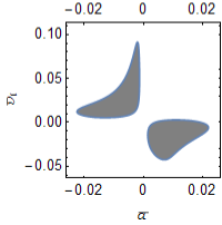
Figure 1: The 92% CL area for the $Z^{\prime}$ couplings: $(\bar{a},\bar{v}_{l})$ plane at $m_{Z^{\prime}}=3$ TeV, $\bar{v}_{u}=5\times 10^{-2}$

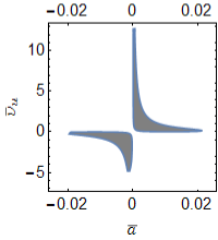
Figure 2: The 92% CL area for the $Z^{\prime}$ couplings: $(\bar{a},\bar{v}_{q})$ plane at $m_{Z^{\prime}}=3$ TeV, $\bar{v}_{l}=5\times 10^{-4}$

We calculate $\Sigma^{SM}$ by means of FEWZ 3 F. Petriello, Ye Li, S. Quackenbush and R. Gavin and $A^{SM}_{FB}$, $\Delta^{SM}$, $\Delta_{1,2}$, and $\Sigma_{1,2}$ – by using Wolfram Mathematica 10 Mat , FeynArts and FormCalc Fey . Some of computations were fulfilled at the Dubna cluster HybriLIT Hyb . The accuracy of all these calculations is considered in detail in Discussion.

The results of the carried out calculations are presented in Table 1. They demonstrate at almost $2\sigma$ CL that the data on the $A_{FB}$ at $\sqrt{s}=7$ and 8 TeV are compatible with the $Z^{\prime}$ existence. The estimates of all the $Z^{\prime}$ couplings to the SM fermions are obtained. The values of parameters $\bar{a}\bar{v}_{l}$ and $\bar{a}\bar{v}_{u}$ are found as independent variables first in the literature.

IV Discussion

We have analyzed the data on the $A_{FB}$ for the Drell-Yan annihilation process at the LHC presented by the CMS collaborations for $\sqrt{s}=7$ TeV The CMS Collaboration (2013) and 8 TeV The CMS Collaboration (2016a) with the goal of estimation in a model-independent approach the couplings of the Abelian $Z^{\prime}$ boson to the SM fermions. The investigation was carried out within the effective Lagrangian 2, 3. As the important ingredient the relations 5 were used. They essentially decreased the number of couplings, which must be fitted, and modified accordingly the kinematics structure of the cross-sections. As a result, the angular distribution of the theoretic cross-section became uniquely determined by this particle. It is important to note that the relations are satisfied at tree-level in all the extended models investigated by the CMS and ATLAS The ATLAS Collaboration (2012) – The CMS Collaboration (2016b) collaborations in the model-dependent approach. They also cover other renormalizable models of Abelian $Z^{\prime}$ Gulov and Skalozub (2010). Due to these constraints, we performed the three-parametric fit of the experimental data and estimated the unknown $\bar{a}^{2}$, $\bar{a}\bar{v}_{l}$ and $\bar{a}\bar{v}_{u}$ couplings for a number of $m_{Z^{\prime}}$.

The maximum likelihood method was applied. The QCD sector was evaluated with an NNLO accuracy, while the electroweak corrections were calculated up to NLO. This is a standard for the Drell-Yan production description at the LHC nowadays. The NLO effects are accounted for by means of an improved Born approximation (IBA). As it is known, the IBA absorbs the majority of NLO electroweak corrections. It is shown in M. Huber (2010) its deviation from exact NLO calculations does not exceed 1-2%. In the IBA approach, the coupling constants are replaced with the effective running couplings which are obtained from the one-loop expressions for the self-energy and vertex corrections. In fact, it means that we use an elastic scattering approximation but in all calculations we replace $\alpha_{em}(0)$ with $\alpha_{em}(m_{Z})$. The PDF uncertainties were estimated by means of the standard formula (see, for example, A.D. Martin, W.J. Stirling, R.S. Thorne, G. Watt (2009))

$$\Delta F=\frac{1}{2}\sqrt{\sum_{k=1}^{n}\left[F\left(S^{+}_{k}\right)-F\left(S^{-}_{k}\right)\right]^{2}},$$ (14)

where $F$ is any quantity which depends on PDFs, $S^{\pm}_{k}$ are the PDF eigenvectors, and summation is performed over all the eigenvectors present in a given PDF set. In Table 2, we show the example for $\Sigma_{k}$ factors in the bin $86\leq M\leq 96$, $0\leq|Y|\leq 1$. From the presented results we see that the PDF uncertainty of the $Z^{\prime}$ cross-sections does not exceed 3%. Finally, considering all the discussed uncertainties as independent, we obtain that total theoretical uncertainty of the $A_{FB}$ predicted by (13) is not larger than 5%.

The uncertainties followed from the statistical and the PDF errors were calculated at $\sim 2\sigma$ CL. It was concluded that the $Z^{\prime}$ existence is admitted by the data on $A_{FB}$ measured by the CMS at $\sqrt{s}=7$ and 8 TeV. The $Z^{\prime}$ signal (hint, in fact) is non-zero at $92\%$ CL. The obtained numerical values for the $Z^{\prime}$ coupling $\bar{v}^{2}_{l}$ are in an agreement with the ones found already for the LEP Gulov and Skalozub (2010) and Tevatron A. Gulov, A. Kozhushko (2011) in a model-independent analysis where other observables were proposed.

It is worth noting that the $\bar{a}\bar{v}_{l}$ coupling and $\bar{a}\bar{v}_{u}$ were estimated directly for the first time. In all other previous analysis only $\bar{v}^{2}_{l}$ could be estimated, while $\bar{a}\bar{v}_{l}$ was suppressed due to the process kinematics. Let us compare those values with our results. The calculation yields $\bar{v}^{2}_{l}<2.8\times 10^{-4}$ which is in agreement with $\bar{v}^{2}_{l}=(2.25^{+1.79}_{-2.07})\times 10^{-4}$ from Gulov and Skalozub (2010) and $\bar{v}^{2}_{l}<1.69\times 10^{-4}$ from A. Gulov, A. Kozhushko (2011). Further, as we see from Table 1, the experimental CMS data at 7 and 8 TeV, which were obtained with different precision, lead to the close values for estimated parameters.

It is essential that the obtained coupling values are weakly dependent on the $Z^{\prime}$ mass. It is caused by the cross-section dependence on this parameter. Really, the factors $\hat{F}_{qk}$ in Eq. 7 depend on the $m_{Z^{\prime}}$ through the $Z^{\prime}$ propagator. This is a denominator effect, which is small at not close to the $Z^{\prime}$ pole position energies. On the contrary, the couplings enter the cross-section through the numerator. Hence, the observables are much more sensitive to the coupling variations.

Now let us turn back to Eq. 4. The current limit on the $Z-Z^{\prime}$ mixing angle from the global fit of the LEP data is about $|\theta_{0}|=10^{-3}-10^{-4}$. We use this value to estimate the $m_{Z^{\prime}}$. Due to 4, $\theta_{0}$ is expressed through $\bar{a}$ and $m_{Z^{\prime}}$. Since $\bar{a}$ is already derived, it is possible to obtain the $m_{Z^{\prime}}$ limits which satisfy the LEP restrictions on $\theta_{0}$. The optimistic estimation is $3<m_{Z^{\prime}}<7-8$ TeV. The experimental lower limit was recently increased to the $m_{Z^{\prime}}>3.5$ TeV in the model-dependent analysis presented by the CMS and ATLAS Collaborations. The $Z^{\prime}$ with such mass is possible to be detected in the future LHC experiments. Nevertheless in this case it will be difficult to distinguish the basic $Z^{\prime}$ model. Therefore the model-independent description becomes an important instrument for investigating this problem. The obtained values of the couplings could be used in the $Z^{\prime}$ model identifications either at present or future colliders.

Finally we compare our results for $\bar{a}^{2}$ with those of in Gulov and Skalozub (2010), A. Gulov, A. Kozhushko (2011), where the data of the LEP and some LHC experiments have been analyzed on the same principles as in the present paper. The essential difference, however, is that in the former case it was possible to introduce a one-parameter observable for estimating the $\bar{a}^{2}$. The $\bar{a}\bar{v_{l}}$ contribution was excluded due to more simple kinematics structure of the lepton cross-sections for the processes $e^{+}e^{-}\to\mu^{+}\mu^{-}(\tau^{+}\tau^{-})$. The $\bar{a}^{2}$ found in Gulov and Skalozub (2010) has the value $\bar{a}^{2}\leq 0.95\times 10^{-3}$ that differs from our result $\bar{a}^{2}=(2.4^{+38.6}_{-1.3})\times 10^{-5}$. This is a universal parameter related due to 4 with the $Z-Z^{\prime}$ mixing angle, which was estimated at LEP experiments Jens Erler, Paul Langacker, Shoaib Munir and Eduardo Rojas (2009). On the contrary, the value of $\bar{a}^{2}$ found in A. Gulov, A. Kozhushko (2011) is one order larger than obtained in Section 3. We could explain this discrepancy by the approximation for the Drell-Yan process cross section used in A. Gulov, A. Kozhushko (2011), which is applicable at energies close to the resonance peak, only. Possibly, this also depends on the data set and observables introduced in the course of the analysis applied.

As conclusion we note that the applied model-independent approach can be used for analyzing data of other experiments. In fact, at the LHC numerous data on different processes have been accumulated. Further improvements of the results is expected from measurements fulfilled at run 2 of the LHC. So, it is of interest to investigate these measurements by the applied method. Besides that, the $Z$ boson generation is perspective where the $Z-Z^{\prime}$ mixing angle $\theta_{0}$ can be estimated and compared with the one obtained in the present paper. We left all these problems for the future.

Appendix A The Plots of the $Z^{\prime}$ Factors

Below we present the behaviour of the cross-section factors introduced in (7) and (8). Here the functions $F_{1}$, $F_{2}$, $F_{3}$, and $F_{4}$ stand for the factors at $\bar{a}^{2}$, $\bar{a}\bar{v}_{l}$, $\bar{a}\bar{v}_{u}$, and $\bar{v}_{l}\bar{v}_{u}$, respectively.

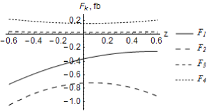
Figure A.1: $F_{k}(M,Y,z)$ factors at $M=50$ GeV, $Y=1.25$

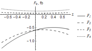
Figure A.2: $F_{k}(M,Y,z)$ factors at $M=60$ GeV, $Y=1.25$

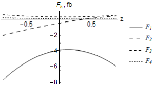
Figure A.3: $F_{k}(M,Y,z)$ factors at $M=80$ GeV, $Y=1.25$

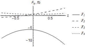
Figure A.4: $F_{k}(M,Y,z)$ factors at $M=100$ GeV, $Y=1.25$

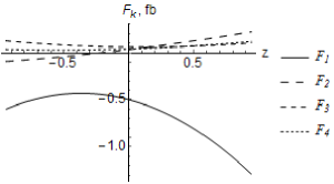
Figure A.5: $F_{k}(M,Y,z)$ factors at $M=120$ GeV, $Y=1.25$

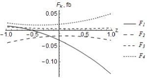
Figure A.6: $F_{k}(M,Y,z)$ factors at $M=200$ GeV, $Y=1.25$

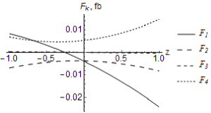
Figure A.7: $F_{k}(M,Y,z)$ factors at $M=400$ GeV, $Y=1.25$

Appendix B On the Relation between the $Z^{\prime}$ Couplings

Below we adduce an information on the derivation of mixing angle 4 and correlations 5. As it was noted in Sect. 2, these correlations are proper to renormalizable models containing the Abelian $Z^{\prime}$ boson. They have been obtained in A. V. Gulov, V. V. Skalozub (2001), A. V. Gulov, V. V. Skalozub (2000) by using two different procedures (see for details Gulov and Skalozub (2010)). General idea of the first approach is mentioned in the main text. The second way is based on principle of gauge invariance with respect to the $\tilde{U}(1)$ transformations A. V. Gulov, V. V. Skalozub (2000).

The most general effective Lagrangian describing the $Z^{\prime}$ interactions with the SM fields and preserving the $SU(2)_{L}\times U(1)_{Y}\times\tilde{U}(1)$ gauge group reads M. Cvetic and B. W. Lynn (1987), G. Degrassi and A. Sirlin (1989),

$$\begin{split}\mathcal{L}=\frac{1}{2}\left|\left(iD^{ew,\phi}_{\mu}+\tilde{g}\tilde{Y}_{\phi}Z^{\prime}_{0\mu}\right)\phi\right|^{2}\\ +\sum\limits_{f_{L}}\bar{f}_{L}\left(iD^{ew,L}_{\mu}+\tilde{g}\tilde{Y}_{f}^{L}Z^{\prime}_{0\mu}\right)\gamma^{\mu}f_{L}\\ +\sum\limits_{f_{R}}\bar{f}_{R}\left(iD^{ew,R}_{\mu}+\tilde{g}\tilde{Y}^{R}_{f}Z^{\prime}_{0\mu}\right)\gamma^{\mu}f_{R},\end{split}$$ (15)

where the summation over all the SM left-handed doublets, $f_{L}$, and the SM right-handed singlets, $f_{R},$ is assumed and $D_{\mu}^{ew,L}=\partial_{\mu}-\frac{ig}{2}\sigma^{a}A^{a}_{\mu}-\frac{ig^{\prime}}{2}Y_{f,L}B_{\mu}$ is the standard model covariant derivative with the values of the hypercharges: $Y_{\phi}=1$ , $Y_{f,L}=\frac{1}{3}$ and $D^{ew,R}_{\mu}=\partial_{\mu}-ig^{\prime}Q_{f}B_{\mu}$, $Q_{f}$ is the fermion charge in the positron charge units, $\sigma^{a}$ are the Pauli matrices. The values of the dimensionless constants $\tilde{Y}_{\phi},\tilde{Y}^{L}_{f},\tilde{Y}^{R}_{f}$ depend on a particular model and here are considered as arbitrary numbers.

The masses of the SM particles are generated by the spontaneous breaking of the $SU(2)_{L}\times U(1)_{Y}\to U(1)_{em}$ symmetry due to the non-zero vacuum value of the scalar doublet. Hence, the mass eigenstates of the vector bosons are appeared to be shifted from the original fields $A^{a}_{\mu},B_{\mu},Z^{\prime}_{0\mu}$ because the corresponding mass matrix became nondiagonal. Physical fields $A_{\mu},Z_{\mu},Z^{\prime}_{\mu}$ are obtained by the orthogonal transformation:

$$B_{\mu} = A_{\mu}c_{W}-(Z_{\mu}c_{0}-Z^{\prime}_{\mu}s_{0})s_{W}$$ (16)

$$A^{3}_{\mu} = A_{\mu}s_{W}+(Z_{\mu}c_{0}-Z^{\prime}_{\mu}s_{0})c_{W}$$

$$Z^{\prime}_{0\mu} = Z_{\mu}s_{0}+Z^{\prime}_{\mu}c_{0},$$

where $c_{W}=\cos\theta_{W},s_{W}=\sin\theta_{W}$ and the SM value of the Weinberg angle $\tan\theta_{W}=g^{\prime}/g$. Whereas $c_{0}=\cos\theta_{0},s_{0}=\sin\theta_{0}$ denote the cosine and sine of the mixing angle $\theta_{0}$ relating the physical states $Z_{\mu},Z^{\prime}_{\mu}$ to the massive neutral components of the $SU(2)_{L}\times U(1)_{Y}\times\tilde{U}(1)$ gauge fields. The value of the $\theta_{0}$ can be determined from the relation

$$\tan^{2}\theta_{0}=\frac{m^{2}_{W}/c^{2}_{W}-m^{2}_{Z}}{m^{2}_{Z^{\prime}}-m^{2}_{W}/c^{2}_{W}},$$ (17)

(see also G. Degrassi and A. Sirlin (1989)) expressing it through the masses of physical states, which appeared after the orthogonalization, and the SM Weinberg agle. The difference in the numerator of the r.h.s. is positive and completely determined by the $Z^{\prime}$ coupling to the scalar field doublet A. V. Gulov, V. V. Skalozub (2000). After the diagonalization, the masses of physical states are given by

$$m^{2}_{A} = 0,$$ (18)

$$m^{2}_{Z} = m_{W}^{2}c_{W}^{-2}\left(1-\frac{4\tilde{g}^{2}\tilde{Y}^{2}_{\phi}}{g^{2}}\frac{m^{2}_{W}}{m^{2}_{Z^{\prime}}-m_{W}^{2}c_{W}^{-2}}\right),$$

$$m^{2}_{Z^{\prime}} = m^{2}_{Z^{\prime}_{0}}+(m_{W}^{2}c_{W}^{-2}-m^{2}_{Z})+\frac{4\tilde{g}^{2}\tilde{Y}^{2}_{\phi}}{g^{2}}m^{2}_{W}.$$

Here, $m_{Z^{\prime}_{0}}$ is the mass of the $Z^{\prime}$ before diagonalization. This value is not specified and is a free parameter. As we see, the mass $m_{Z}$ differs from the SM value $m_{W}/c_{W}$ by a small quantity of the order $\sim m^{2}_{W}/m^{2}_{Z^{\prime}}$. So the mixing angle 17 is also small, $\theta_{0}\sim m^{2}_{W}/m^{2}_{Z^{\prime}}$ Using 16 the Lagrangian of the model can be expressed in terms of the physical fields. The $\theta_{0}$-dependent terms generate new interactions originally absent in 15. Here it worth reminding that in calculations carried out we used the SM value of the Weinberg angle $\tan\theta_{W}=g^{\prime}/g$.

To derive the correlations 5 we require the Yukawa terms of the SM to be invariant with respect to the $\tilde{U}(1)$ gauge symmetry. This condition is fulfilled if the relation holds

$$\tilde{Y}^{R}_{f}=\tilde{Y}^{L}_{f}+2T^{3}_{f}~{}\tilde{Y}_{\phi}.$$ (19)

Introducing the $Z^{\prime}$ interaction constants with the vector and axial-vector currents of fermions $v_{Z^{\prime}}^{f}=\frac{\tilde{g}}{2}(\tilde{Y}^{L}_{f}+\tilde{Y}^{R}_{f}),~{}a_{Z^{\prime}}^{f}=\frac{\tilde{g}}{2}(\tilde{Y}^{L}_{f}-\tilde{Y}^{R}_{f})$ we can rewrite 19 in the form 5. These correlations also hold in Two-Higgs-Doublets SM A. V. Gulov, V. V. Skalozub (2001), Gulov and Skalozub (2010).

The relation 19 is just as in the SM for the given proper values of the hypercharges $Y^{R}_{f},Y^{L}_{f},Y_{\phi}.$ In the extended models, the originally independent parameters $\tilde{Y}^{R}_{f},\tilde{Y}^{L}_{f},\tilde{Y}_{\phi}$ have to be connected ones. The fermion and the scalar sectors of the $Z^{\prime}$ physics are correlated. In particular, the mixing angle is simply related with the universal axial vector coupling $a_{f}^{2}$.

Appendix C PDF uncertainties

In this Appendix, we present table which illustrates calculation of the PDF uncertainties with Eq. (14). It shows the $Z^{\prime}$ factors $\Sigma_{k}$ integrated over the bin $86\leq M\leq 96$, $0\leq|Y|\leq 1$ with some of the PDF eigenvectors:

$$\Sigma_{k}=\int_{86~{}GeV}^{96~{}GeV}{dM\int_{-1}^{1}dY\,\Sigma_{k}(M,Y)}.$$

$\Sigma_{k}(M,Y)$ are defined in (12), and $\langle\Sigma\rangle$ means the central values.

Table 2: The $Z^{\prime}$ factors calculated with different PDF eigenvectors and integrated over $86\leq M\leq 96$, $0\leq|Y|\leq 1$

	$\Sigma_{1}$, pb	$\Sigma_{2}$, pb	$\Sigma_{3}$, pb	$\Sigma_{4}$, pb
1	$-3366.02$	$200.44$	$205.64$	$1.96$
2	$-3364.16$	$200.31$	$205.59$	$1.96$
3	$-3364.55$	$200.50$	$207.17$	$1.95$
4	$-3365.51$	$200.27$	$204.30$	$1.97$
5	$-3373.87$	$200.62$	$207.58$	$1.98$
6	$-3358.97$	$200.21$	$204.23$	$1.96$
7	$-3369.25$	$200.91$	$206.24$	$1.97$
8	$-3362.64$	$200.06$	$205.23$	$1.96$
9	$-3414.86$	$203.46$	$208.02$	$2.00$
10	$-3323.79$	$197.83$	$203.62$	$1.94$
11	$-3362.33$	$200.58$	$210.16$	$1.94$
12	$-3365.90$	$200.28$	$203.90$	$1.97$
13	$-3350.05$	$199.40$	$204.09$	$1.95$
14	$-3374.68$	$201.01$	$206.62$	$1.97$
15	$-3359.04$	$200.06$	$205.05$	$1.96$
16	$-3354.31$	$199.71$	$205.13$	$1.96$
17	$-3366.81$	$200.26$	$206.29$	$1.97$
18	$-3361.63$	$200.50$	$204.53$	$1.96$
19	$-3360.79$	$200.18$	$205.07$	$1.96$
20	$-3345.18$	$199.14$	$204.75$	$1.95$
$\langle\Sigma\rangle$, pb	$-3365.09$	$200.37$	$205.61$	$1.96$
$\frac{\Delta\Sigma}{\langle\Sigma\rangle}$, %	$1.6$	$1.4$	$2.6$	$2.1$

References

- A. Leike (1999) A. Leike, Phys. Rept. 317, 143 (1999), arXiv:9805494 [hep-ph] .
- Accomando, Elena and Belyaev, Alexander and Fedeli, Luca and King, Stephen F. and Shepherd-Themistocleous, Claire (2011) Accomando, Elena and Belyaev, Alexander and Fedeli, Luca and King, Stephen F. and Shepherd-Themistocleous, Claire, Phys. Rev. D83, 075012 (2011), arXiv:1010.6058 [hep-ph] .
- J. Alcaraz, P. Azzurri, A. Bajo-Vaquero et al. (2007) J. Alcaraz, P. Azzurri, A. Bajo-Vaquero et al., A Combination of Preliminary Electroweak Measurements and Constraints on the Standard Model, Tech. Rep. CERN-PH-EP/2006-042 (The LEP Collaborations, 2007) arXiv:1009.2320 [hep-ph] .
- The OPAL Collaboration, G. Abbiendi et al. (2004) The OPAL Collaboration, G. Abbiendi et al., Eur. Phys. J. C 33, 173 (2004), arXiv:0309053 [hep-ex] .
- The DELPHI Collaboration, J. Abdallah et al. (2006) The DELPHI Collaboration, J. Abdallah et al., Eur. Phys. J. C 45, 589 (2006), arXiv:0512012 [hep-ex] .
- A. Ferroglia, A. Lorca, J.J. van der Bij (2007) A. Ferroglia, A. Lorca, J.J. van der Bij, Annalen Phys. 16, 563 (2007), arXiv:0611174 [hep-ph] .
- P. Osland, A. A. Pankov and A. V. Tsytrinov (2010) P. Osland, A. A. Pankov and A. V. Tsytrinov, Eur. Phys. J. C 67, 191 (2010), arXiv:0912.2806 [hep-ph] .
- T. Han, P. Langacker, Z. Liu and L.-T. Wang (2013) T. Han, P. Langacker, Z. Liu and L.-T. Wang, “Diagnosis of a New Neutral Gauge Boson at the LHC and ILC for Snowmass 2013,” (2013), arXiv:1308.2738 [hep-ph] .
- Gulov and Skalozub (2010) A. Gulov and V. Skalozub, Int. J. Mod. Phys. A 25, 5787 (2010), arXiv:1009.2320 [hep-ph] .
- A. V. Gulov, V. V. Skalozub (2001) A. V. Gulov, V. V. Skalozub, Int. J. Mod. Phys. A 16, 179 (2001).
- A. V. Gulov, V. V. Skalozub (2000) A. V. Gulov, V. V. Skalozub, Eur. Phys. J. C 17, 685 (2000), arXiv:0004038v2 [hep-ph] .
- The CMS Collaboration (2013) The CMS Collaboration, Phys. Lett. B 718, 752 (2013), arXiv:1207.3973 [hep-ex] .
- The CMS Collaboration (2016a) The CMS Collaboration, Eur. Phys. J. C 76, 325 (2016a), arXiv:1601.04768v2 [hep-ex] .
- The CMS Collaboration (2015) The CMS Collaboration, “Complementarity of Forward-Backward Asymmetry for discovery of Z’ bosons at the Large Hadron Collider,” (2015), arXiv:1510.05892 [hep-ph] .
- Jens Erler, Paul Langacker, Shoaib Munir and Eduardo Rojas (2009) Jens Erler, Paul Langacker, Shoaib Munir and Eduardo Rojas, Journal of High Energy Physics 2009, 017 (2009), arXiv:0906.2435 [hep-ph] .
- J. Collins (1977) J. Collins, Phys. Rev. D 16, 2219 (1977).
- G. Degrassi and A. Sirlin (1989) G. Degrassi and A. Sirlin, Phys. Rev. D 40, 3066 (1989).
- M. Cvetic and B. W. Lynn (1987) M. Cvetic and B. W. Lynn, Phys. Rev. D 35, 51 (1987).
- (19) F. Petriello, Ye Li, S. Quackenbush and R. Gavin, “FEWZ 3.0,” http://gate.hep.anl.gov/fpetriello/FEWZ.html.
- (20) “Wolfram Mathematica,” http://www.wolfram.com/.
- (21) “FeynArts,” http://www.feynarts.de/.
- (22) “LIT/JINR heterogeneous cluster,” http://hybrilit.jinr.ru/.
- The ATLAS Collaboration (2012) The ATLAS Collaboration, JHEP 138, 1211 (2012), arXiv:1209.2535v3 [hep-ex] .
- The CMS Collaboration (2016b) The CMS Collaboration, Phys. Rev. D 93, 012001 (2016b), arXiv:1506.03062v2 [hep-ex] .
- M. Huber (2010) M. Huber, “Radiative corrections to the neutral-current Drell-Yan process,” https://www.freidok.uni-freiburg.de/dnb/download/7848 (2010).
- A.D. Martin, W.J. Stirling, R.S. Thorne, G. Watt (2009) A.D. Martin, W.J. Stirling, R.S. Thorne, G. Watt, Eur. Phys. J. C 63, 189 (2009), arXiv:0901.0002v3 [hep-ph] .
- A. Gulov, A. Kozhushko (2011) A. Gulov, A. Kozhushko, Int. J. Mod. Phys. A 26, 4083 (2011), arXiv:1105.3025 [hep-ph] .