Anisotropies of Gravitational-Wave Standard Sirens as a New Cosmological Probe without Redshift Information

Abstract

Gravitational waves (GWs) from compact binary stars at cosmological distances are promising and powerful cosmological probes, referred to as the GW standard sirens. With future GW detectors, we will be able to precisely measure source luminosity distances out to a redshift $z\sim 5$. To extract cosmological information, previously proposed cosmological studies using the GW standard sirens rely on source redshift information obtained through an extensive electromagnetic follow-up campaign. However, the redshift identification is typically time consuming and rather challenging. Here, we propose a novel method for cosmology with the GW standard sirens free from the redshift measurements. Utilizing the anisotropies of the number density and luminosity distances of compact binaries originated from the large-scale structure, we show that, once GW observations will be well established in the future, (i) these anisotropies can be measured even at very high redshifts ($z\geq 2$), where the identification of the electromagnetic counterpart is difficult, (ii) the expected constraints on the primordial non-Gaussianity with the Einstein Telescope would be comparable to or even better than the other large-scale structure probes at the same epoch, and (iii) the cross-correlation with other cosmological observations is found to have high-statistical significance, providing additional cosmological information at very high redshifts.

Introduction.— First detection of gravitational waves (GW) by the advanced laser interferometer, aLIGO, has opened a new window to probe unseen Universe LIGO Scientific Collaboration and Virgo Collaboration (2016). With a network of detectors including aVIRGO and KAGRA Evans (2014), the GW would become a powerful and promising tool to probe cosmology and astrophysics, complementary to or even independent of the electromagnetic observations. Indeed, the future ground- and space-based GW experiments such as the Einstein Telescope (ET) Punturo et al. (2010), 40-km LIGO Dwyer et al. (2015), eLISA Seoane et al. (2013), and DECIGO Sato et al. (2009), are planning to realize much higher sensitivity, with which we can observe a large number of neutron star (NS) binaries at cosmological distances. One important aspect of future GW observations is that one would be able to measure the luminosity distance to each binary source (so-called standard sirens) with an unprecedented precision, from which the cosmic expansion history can be accurately determined, e.g., Refs.  Schutz (1986); Petiteau et al. (2011); Cutler and Holz (2009); Nishizawa et al. (2011); Sathyaprakash et al. (2010); Taylor and Gair (2012). In addition, measurements of these GWs will be very useful to study the gravitational lensing effect induced by the Large-Scale Structure (LSS) by looking at the anisotropies of the observed luminosity distances Cutler and Holz (2009); Hirata et al. (2010); Shang and Haiman (2011); Camera and Nishizawa (2013). The use of the LSS-induced anisotropies on other cosmological probes has been also studied in Refs. Cooray et al. (2006); McQuinn and White (2013) in different context.

Nevertheless, one crucial assumption behind these studies is that redshift information or a corresponding distance measure other than luminosity distance are a priori known because GW observation alone is not sensitive to source redshift. However, the source identification and redshift measurement with electromagnetic (EM) follow-up observations are rather challenging, and extensive follow-up campaigns are required. In particular, the EM observation to identify the host galaxy of each compact binary would be very difficult at higher redshifts Nissanke et al. (2013), and the feasibility of source identification largely depends on the emission mechanism of the EM counterparts. As discussed in Nishizawa et al. (2012), the success rate of identification is estimated to be $\sim 10^{-4}$ from galaxy catalogs of future surveys and $\sim 10^{-3}$ from coincident searches of short gamma-ray bursts with gamma-ray telescopes. To circumvent the situations, alternative methods have been proposed. Reference MacLeod and Hogan (2008) presents a statistical method without identifying an EM counterpart, assuming a redshift distribution based on a complete galaxy catalog. References Messenger and Read (2012); Taylor et al. (2012) assume the equation of state of neutron stars and/or a narrow distribution of NS mass to infer the redshift of each source. However, the reliability of redshift estimation largely depends on the underlying assumptions.

In this Letter, we propose a novel approach to pursue the cosmology with the GW standard sirens without any assumptions for redshift information. The proposed method is to utilize anisotropies in the observables induced by the LSS. The distribution function is anisotropic due to the clustering of the NS binaries by the fluctuations of the gravitational potential. The LSS also induces the gravitational lensing, and the measured luminosity distance is modified. These anisotropic signals contain rich cosmological information helpful to constrain the cosmic expansion history and structure formation. One remarkable difference from the previous studies is that the present method directly offers a redshift-free measurement of the anisotropies at high statistical significance. The measured signal is expected to be powerful to constrain cosmology especially at the distant universe. In the followings, we discuss how the LSS induces the anisotropies in the observables constructed from GW signals.

Anisotropies induced by the LSS.— An observable considered in this Letter is a distribution of NS binaries per luminosity distance $N(D,\Omega)$ as a function of their luminosity distance $D$ and direction $\Omega$. Hereafter, we denote the arguments by $\bm{x}=(D,\Omega)$. We then define a normalized distribution function, $p(\bm{x})\equiv N(\bm{x})/\int{\rm d}DN(\bm{x})$. At each angular pixel, observed binaries are divided into subsamples according to their luminosity distance. We denote, respectively, by $D_{i}^{\rm max}$ and $D_{i}^{\rm min}$ the maximum and minimum values of the observed luminosity distance in $i$th luminosity distance bin.

There are two types of LSS-induced anisotropies in the observables. The clustering of the NS binaries at each direction causes the fluctuations in $N(\bm{x})$. The observed luminosity distance $D$ should also have explicit directional dependence by the gravitational lensing of the LSS, and is related to the original luminosity distance $\overline{D}$ (in the absence of the lensing effect) through (e.g., Refs. Futamase and Sasaki (1989); Hirata et al. (2010))

$$D(\bm{x})=\overline{D}[1+\kappa(\overline{\bm{x}})]\;,\quad(\overline{\bm{x}}=(\overline{D},\Omega))\,.$$ (1)

The quantity $\kappa(\bm{x})$ is the lensing convergence induced by the gravitational potential of the LSS. The lensing effect on the trajectory of GW propagation is at second order in $\kappa$, and is ignored in the following derivation.

To discuss the feasibility of measuring the anisotropies from the LSS, we construct an estimator based on the observed luminosity distance. First, we may take the average of $D$ within the $i$th luminosity-distance bin at each angular direction $\Omega$:

$$\widehat{d}_{i}(\Omega) ={\int_{D_{i}^{\rm min}}^{D_{i}^{\rm max}}\!\!{\rm d}{D}\,}D\,p(\bm{x})\,.$$ (2)

Further averaging $\widehat{d}_{i}(\Omega)$ over the entire sky, we obtain a mean luminosity distance $\widehat{d}_{i}$ at the $i$th bin. We then estimate the fluctuation in the $i$th luminosity-distance bin at each direction by taking the difference $\widehat{d}_{i}(\Omega)-\widehat{d}_{i}$. Thus, a simple dimensionless estimator for the LSS-induced anisotropies $\widehat{s}$ is introduced:

$$\widehat{s}_{i}(\Omega) \equiv\frac{\widehat{d}_{i}(\Omega)-\widehat{d}_{i}}{\widehat{d}_{i}}\,.$$ (3)

This quantity is proportional to the number density of the NS binaries, and also probes the lensing modification to the luminosity distance. Therefore, the above quantity is one of the estimators to probe the LSS anisotropies of both the clustering and lensing.

To understand how the estimator $\widehat{s}_{i}$ is sensitive to the cosmology, we rewrite Eq. (3) in terms of the fluctuations of the number density $\delta$ and lensing convergence field $\kappa$ generated by the LSS. Here and in what follows, we consider the terms up to the first order of $\delta$ and $\kappa$. Unlike the methods using the source redshift information, the source distribution is given as a function of the observed luminosity distance. Let us recall that the observed number distribution is modified by the lensing effect. It is related to the unlensed binary distribution $\overline{p}$ through the number conservation

$$p(\bm{x})\,{\rm d}\Omega\,{\rm d}D=\overline{p}(\overline{D})[1+\delta(\overline{\bm{x}})]\,{\rm d}\Omega\,{\rm d}\overline{D}\,.$$ (4)

Here the fluctuations of the unlensed quantity $\delta(\overline{\bm{x}})$ come from the effect of the NS-binary clustering. Introducing a dimensionless quantity $n(\bm{x})\equiv Dp(\bm{x})$, the above equation implies

$$n(\bm{x})=({\rm d}\overline{D}/{\rm d}D)[1+\kappa(\overline{\bm{x}})]\overline{n}(\overline{D})[1+\delta(\overline{\bm{x}})]$$

$$\quad\simeq[1-D\kappa^{\prime}(\bm{x})]\overline{n}[D/(1+\kappa(\bm{x}))][1+\delta(\bm{x})]\,.$$ (5)

where the prime denotes the derivative with respect to $D$, and we use Eq. (1) and ignore higher-order terms of the fluctuations. Substituting the above equation into Eq. (2), we find

$$\widehat{d}_{i}(\Omega)={\int_{D_{i}^{\rm min}}^{D_{i}^{\rm max}}\!\!{\rm d}{D}\,}\overline{n}\left[\frac{D}{1+\kappa(\bm{x})}\right][1+\delta(\bm{x})-D\kappa^{\prime}(\bm{x})]\,.$$ (6)

Averaging $\widehat{d}_{i}(\Omega)$ over all directions $\Omega$, we obtain a theoretical expression for the averaged luminosity distance as

$$\widehat{d}_{i} ={\int_{D_{i}^{\rm min}}^{D_{i}^{\rm max}}\!\!{\rm d}{D}\,}\overline{n}(D)\equiv\overline{d}_{i}\,.$$ (7)

Note that we implicitly assumed that the average of $\kappa(\bm{x})$ over the entire sky becomes zero. On the other hand, the luminosity-distance anisotropies are obtained by expanding Eq. (6) upto first order of $\kappa$ and $\delta$ as

$$\widehat{d}_{i}(\Omega)\simeq\overline{d}_{i}+{\int_{D_{i}^{\rm min}}^{D_{i}^{\rm max}}\!\!{\rm d}{D}\,}\overline{n}(D)[\delta(\bm{x})+\gamma(D)\kappa(\bm{x})]\,.$$ (8)

Here we define $\gamma(D)\equiv 1+D[\delta_{\rm D}(D-D_{i}^{\rm min})-\delta_{\rm D}(D-D_{i}^{\rm max})]$ with $\delta_{\rm D}$ being the delta function. The above equation leads to

$$\widehat{s}_{i}(\Omega) =\frac{1}{\overline{d}_{i}}{\int_{D_{i}^{\rm min}}^{D_{i}^{\rm max}}\!\!{\rm d}{D}\,}\overline{n}(D)[\delta(\bm{x})+\gamma(D)\kappa(\bm{x})]\,.$$ (9)

The anisotropic signal $\widehat{s}_{i}$ statistically contains rich cosmological information. To extract the information, we may move to the harmonic space, and define the angular power spectrum, $\widehat{C}^{s_{i}s_{j}}_{\ell}\equiv\sum_{m=-\ell}^{\ell}(\widehat{s}_{i,\ell m}\widehat{s}_{j,\ell m}^{*}+{\rm c.c.})/[2(2\ell+1)]$, where $\widehat{s}_{i,\ell m}$ is the spherical harmonic coefficient of the signal. Taking the ensemble average of this, the power spectrum is theoretically expressed as

$$C^{s_{i}s_{j}}_{\ell}\equiv\langle\widehat{C}^{s_{i}s_{j}}_{\ell}\rangle={\int_{D_{i}^{\rm min}}^{D_{i}^{\rm max}}\!\!\frac{{\rm d}{D_{1}}}{\overline{d}_{i}}\,}{\int_{D_{j}^{\rm min}}^{D_{j}^{\rm max}}\!\!\frac{{\rm d}{D_{2}}}{\overline{d}_{j}}\,}$$

$$\qquad\times\overline{n}(D_{1})\overline{n}(D_{2})\bigg{\{}C_{\ell}^{\delta_{1}\delta_{2}}+\gamma(D_{1})\gamma(D_{2})\,C_{\ell}^{\kappa_{1}\kappa_{2}}$$

$$\qquad\qquad+\gamma(D_{1})\,C_{\ell}^{\delta_{2}\kappa_{1}}+(1\leftrightarrow 2)\bigg{\}}\,.$$ (10)

Here, $C_{\ell}^{\delta\delta}$, $C_{\ell}^{\delta\kappa}$, and $C_{\ell}^{\kappa\kappa}$ are the auto and cross angular power spectra of the number density fluctuations and lensing convergence, given by $\langle X_{\ell m}(D_{1})Y^{*}_{\ell^{\prime}m^{\prime}}(D_{2})\rangle=\delta_{\ell\ell^{\prime}}\delta_{mm^{\prime}}\,C_{\ell}^{X_{1}Y_{2}}$, with $X$ and $Y$ being either $\delta$ or $\kappa$. The information on the cosmic expansion and the growth of structure is encapsulated in these power spectra. In computing the above quantities theoretically, we need to know the unlensed binary distribution $\overline{n}(\overline{D})$, which is not the actual observable. At first order in $\delta$ and $\kappa$, however, it can be estimated by averaging the observed distribution over the entire sky.

Signal-to-noise ratio.— Feasibility to measure the power spectrum largely depends on the noise properties of $\widehat{s}_{i}$. One important noise is the measurement error of the luminosity distance coming from the limited sensitivity of the GW detector. Let us denote this measurement error for each source by $\epsilon=\delta D/D$. For simplicity, we assume that $\epsilon$ is the random Gaussian field with zero mean, independently of the angular position, and it does not correlate between different GW sources. The magnitude of the error $\epsilon$ does actually depend not only on the detector sensitivity but also on how far each GW source is. To estimate the expected size of $\epsilon$, we consider the ET, and adopt the sky-averaged sensitivity in Ref. Regimbau et al. (2012). For each binary source, we assume the restricted $1.5$ post-Newtonian waveform, setting the spin parameter to zero. Then, the size of the error $\epsilon$ is estimated as a function of luminosity distance based on the Fisher matrix analysis presented in Ref. Nishizawa et al. (2012).

Once we obtained the error $\epsilon$, we propagate it to the noise of LSS-induced anisotropies as follows. Ignoring the LSS effects, the measured luminosity distance is given by $D=\overline{D}(1+\epsilon)$. This produces an error in the luminosity distance of Eq. (2), as

$$\delta\widehat{d}_{i}(\Omega) ={\int_{D_{i}^{\rm min}}^{D_{i}^{\rm max}}\!\!{\rm d}{D}\,}\{\overline{n}(D)-\overline{n}[D/(1+\epsilon)]\}$$

$$\simeq{\int_{D_{i}^{\rm min}}^{D_{i}^{\rm max}}\!\!{\rm d}{D}\,}\overline{n}^{\prime}(D)\,D\,\epsilon+\mathcal{O}(\epsilon^{2})\,.$$ (11)

On the other hand, the noise in the mean distance $\widehat{d}_{i}$, obtained by further averaging $\widehat{d}_{i}(\Omega)$ over the entire sky, would be of the second order of $\epsilon$, and it can be ignored. Thus, from Eq. (3), the noise in $\widehat{s}$ is estimated to be $\delta\widehat{s}_{i}(\Omega)\simeq\delta\widehat{d}_{i}(\Omega)/\overline{d}_{i}$. This produces a shot noiselike contribution, and leads to a systematic offset in the power spectrum, i.e., $\langle\widehat{C}_{\ell}^{s_{i}s_{j}}\rangle\to C^{s_{i}s_{j}}_{\ell}+\delta_{ij}\,(\sigma^{2}_{i}/N_{i})$, where $\sigma^{2}_{i}$ is defined by

$$\sigma_{i}^{2}=\frac{1}{\overline{d}_{i}^{2}}{\int_{D_{i}^{\rm min}}^{D_{i}^{\rm max}}\!\!{\rm d}{D}\,}\overline{p}(D)\left[\frac{\overline{n}^{\prime}(D)}{\overline{p}(D)}\right]^{2}D^{2}\sigma^{2}(D)\,.$$ (12)

with $\sigma(D)$ being the rms of $\epsilon$ estimated based on the Fisher matrix. The $N_{i}$ is the mean number density of GW sources per steradian at $i$th bin.

Note that the uncertainty coming from the above contribution still remains nonvanishing even if we subtract the mean value from the measured power spectrum, and thus needs to be properly taken into account in the statistical analysis. Hence, including further the uncertainty coming from the cosmic variance, the cumulative signal-to-noise ratio (SNR) for the LSS-induced anisotropies at the $i$th bin $\widehat{s}_{i}$ is defined by

$$\left(\frac{S}{N}\right)^{2}_{<\ell} \equiv\sum_{\ell}\frac{2\ell+1}{2}\left[\frac{C^{s_{i}s_{i}}_{\ell}}{(\sigma^{2}_{i}/N_{i})+C^{s_{i}s_{i}}_{\ell}}\right]^{2}\,.$$ (13)

Note that the key inputs to determine SNR are $\sigma(D)$ and $p(D)$.

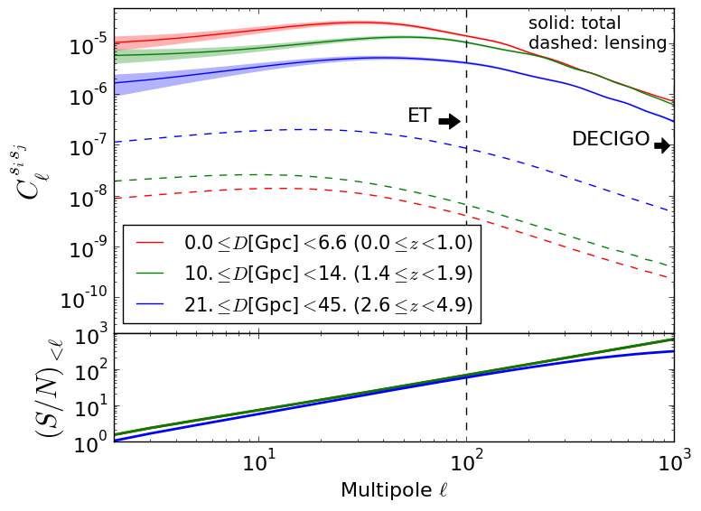
Figure 1: Angular auto-power spectra with expected $1\sigma$ statistical errors (top) and the cumulative SNR of the LSS-induced anisotropies (bottom) with $\Delta\ell=1$. Assuming the three-year observation with the ET, we divide measured luminosity distances into five contiguous bins with equal number of binary sources. The angular power spectrum and SNR is then computed, and plotted as a function of the maximum multipole, $\ell_{\rm max}$. The dashed lines show the lensing contributions. The vertical axis at $\ell=100$ corresponds to the angular resolution of the ET while the resolution of DECIGO is approximately $\ell=1000$.

Figure 1 shows the angular power spectrum and SNR of the LSS-induced anisotropies $\widehat{s}_{i}$ at each luminosity distance bin, plotted against maximum multipoles used in the analysis. Here, we divide measured luminosity distances into five bins with equal number of binary sources, among which the results at representative three bins are particularly shown. The power spectra $C_{\ell}^{s_{i}s_{i}}$ are computed with the CMB Boltzmann code CAMB Lewis et al. (2000), assuming the flat Lambda-CDM model with fiducial cosmological parameters consistent with the seven-year WMAP results Komatsu et al. (2011), using Halofit for computing the non-linear matter power spectrum Smith et al. (2003); Takahashi et al. (2012). The number distribution of binaries is computed using the fitting formula for the NS-NS merger rate in Ref. Cutler and Harms (2006) normalized by the current merger rate, $\dot{n}_{0}=10^{-6}$ Mpc^-3yr^-1 Abadie et al. (2010), which is an intermediate value among several predictions. The power spectrum of the number density fluctuation is computed using a linear bias model with a redshift dependence, parametrized by $b(z)=b_{0}+b_{z}/\mathcal{D}$, where $\mathcal{D}$ is the growth function Yamamoto et al. (2006); Namikawa et al. (2011). The fiducial values of the bias parameters are $b_{0}=b_{z}=1$. The resultant SNRs in Fig. 1 are increased monotonically up to $\ell>1000$ and they look quite similar. With enough angular resolution of GW detectors, the detection of the LSS-induced anisotropies is highly anticipated out to rather distant sources.

To better resolve the source position, however, we at least need three ET-like detectors at different sites. This situation may be optimistic, but has been assumed in the previous studies using EM counterparts of GW sources. Indeed, the determination of the source position is indispensable for the cosmology with standard sirens, and we just follow the assumption of three ET-like detectors at the same sites as aLIGO and VIRGO. Then, based on Ref. Sidery et al. (2014), the angular resolutions for GW sources at $z=1$, $2$, and $3$ are estimated to be $\sim 2.0$, $3.2$, and $3.3\,{\rm deg}$, respectively. The corresponding maximum multipoles become $\ell_{\rm max}\sim 90$, $57$, and $54$. Thus, a network of ET-like detectors is sufficient to provide an opportunity to constrain cosmology even at higher redshifts. This is rather contrasted to the previous study using redshift information, since identification of EM counterparts becomes harder as increasing the redshift. Since the SNR is limited by the cosmic variance, the estimated value of SNR at $\ell_{\rm max}\sim 100$ almost remains the same, irrespective of the uncertainties in the overall merger rate and $\sigma(D)$. Note that for the space-based GW detector like DECIGO, the angular resolution would be much better even at $z>2$, and down to $\sim 0.027$ deg² ($\ell_{\rm max}\sim 1000$) Cutler and Holz (2009).

Cosmological implications — A statistically significant detection of the LSS-induced anisotropies has a potential to tightly constrain cosmology. Since the signal is expected to be statistically high even at distant luminosity distance bins (i.e., high redshift), the LSS-induced anisotropies would be powerful to constrain the early cosmic evolution. One interesting application may be the primordial non-Gaussianity, which can be imprinted on the large-scale clustering at higher redshifts through the scale-dependent galaxy bias (e.g., Refs. Dalal et al. (2008); Slosar et al. (2008)). The leading-order effect of the primordial non-Gaussianity is characterized by the parameter $f_{\rm NL}$ Komatsu and Spergel (2001), and by looking at LSS-induced anisotropies at lower multipoles, a strong constraint on $f_{\rm NL}$ will be obtained. Taking a full covariance matrix of the LSS-induced signals $\widehat{s}_{i}$ up to $\ell_{\rm max}=100$, we estimate the expected constraints on the $f_{\rm NL}$ based on the Fisher matrix analysis. To be specific, in the Fisher matrix, we consider the five luminosity-distance bins as demonstrated in Fig. 1. We only marginalize three parameters $f_{\rm NL}$, $b_{0}$, and $b_{z}$, and compute the expected 1$\sigma$ errors. Note that degeneracy between $f_{\rm NL}$ and other cosmological parameters are very weak and we consider only these parameters Namikawa et al. (2011). The Fisher matrix analysis reveals that the marginalized error $\sigma(f_{\rm NL})=0.54$. This constraint is roughly comparable to or even better than those obtained from the future LSS surveys Carbone et al. (2008). Discarding the two-distant bins still leads to a severe constraint, $\sigma(f_{\rm NL})=1.2$, indicating that primordial non-Gaussianity will be robustly constrained irrespective of a large uncertainty in the binary distribution.

The LSS-induced anisotropies would be also useful for cross-correlation studies with other cosmological probes. The interesting counterpart of the cross correlation would be the gravitational lensing of the cosmic microwave background (CMB) and weak lensing signals from galaxy surveys. Among the two contributions in the LSS-induced anisotropies of standard sirens [see Eq. (9)], the former cross correlation picks up the clustering term in the luminosity distance anisotropies, and it provides a tomographic view of the galaxy clustering at higher redshifts. We find that the SNR at the most distant bin would be $31$ and $43$ combined with the Planck Planck Collaboration (2015) and CMB Stage-IV Abazajian et al. (2015), respectively. On the other hand, the latter cross correlation enables us to extract the pure lensing signals in the luminosity distance anisotropies, since the clustering term in Eq. (9) is mostly uncorrelated between different redshifts. With the future lensing measurement by Euclid The Euclid Theory Working Group (2013), the SNR is found to be 16.

Discussion.— So far, we have considered the NS binaries as the representative GW standard sirens, but the proposed method can be also applied to other GW sources which are not necessarily accompanied by EM counterparts. Examples are black-hole (BH) binaries and NS-BH binaries Abadie et al. (2010). Combining these binaries with NS binaries would certainly increase the SNR of the LSS-induced anisotropies, further improving constraining power on cosmology.

Potential systematics to the LSS-induced anisotropies may come from the luminosity distance estimation to each GW source. In our analysis, the luminosity distance error was estimated based on the averaged GW waveform over the inclination angle of NS binary, assuming the isotropic antenna pattern averaged over the sky. The antenna pattern of a GW detector is, however, anisotropic, and needs to be properly taken into account in practical data analysis. Further, the nonvanishing inclination of the NS binary is known to produce a strong parameter degeneracy with the luminosity distance Nissanke et al. (2010). This degeneracy can increase the measurement uncertainty in the luminosity distance especially for low SNR GW sources, potentially leading to a biased estimation of the anisotropic signal. Following Ref. Nissanke et al. (2010), we estimate the increase of the uncertainty in the luminosity distance due to the degeneracy, and find that the uncertainty increases at most by a factor of 2. Since the detection significance of the LSS-induced anisotropies is almost determined by the cosmic variance, the degeneracy has negligible impact on our results.

Summary.— We proposed a novel method to probe cosmology from the GW standard sirens without redshift information. A key observable is the anisotropies in the number distribution and luminosity distances to each GW source, arising from the clustering and lensing effect of the LSS. Based on a simple estimator given at Eq. (3), feasibility to detect the LSS-induced anisotropies has been discussed, and we found that, via a network of ET-like detectors, once GW observations will be well established in the future,

• The anisotropies at very high redshift ($z>2$) can be detected at high statistical significance (SNR$\gtrsim 100$)

• Constraining power on the primordial non-Gaussianity is roughly comparable to or even better than those from the future LSS surveys,

• Cross correlation with other cosmological probes such as CMB and galaxy weak lensing would be also detectable at high significance by combining future CMB experiments and galaxy surveys observing at the same epoch.

Albeit simple, the present method offers a direct way to probe cosmology only from the GW measurement, and this would provide new insight into the formation and evolution of large-scale structure, definitely complementary to the EM observations.

Note added.— After our paper was accepted, the first detection of GW from binary BH has been reported LIGO Scientific Collaboration and Virgo Collaboration (2016), and this enlarges the future prospect for measuring anisotropic signals. First, the detection suggests a rather higher merger rate for binary BHs, $2$–$400$ Gpc^-3 yr^-1, indicating that even the second-generation GW detectors have a potential to detect the anisotropies of binary BH sources. A high merger rate also suggests that a large number of binary BH will be observed at milli-Hz band, and with the eLISA, most of the extra-galactic sources will be spatially resolved Sesana (2016) (see Seto (2016) for Galactic BH binaries). This implies that in an optimistic case, a single ET-like detector is sufficient to detect the anisotropic signals in combination with the eLISA measurements.