Abstract

This paper proposes a new fast and stable algorithm for the reconstruction of the plasma boundary from discrete magnetic measurements taken at several locations surrounding the vacuum vessel. The resolution of this inverse problem takes two steps. In the first one we transform the set of measurements into Cauchy conditions on a fixed contour $\Gamma_{O}$ close to the measurement points. This is done by least square fitting a truncated series of toroidal harmonic functions to the measurements. The second step consists in solving a Cauchy problem for the elliptic equation satisfied by the flux in the vacuum and for the overdetermined boundary conditions on $\Gamma_{O}$ previously obtained with the help of toroidal harmonics. It is reformulated as an optimal control problem on a fixed annular domain of external boundary $\Gamma_{O}$ and fictitious inner boundary $\Gamma_{I}$. A regularized Kohn-Vogelius cost function depending on the value of the flux on $\Gamma_{I}$ and measuring the discrepency between the solution to the equation satisfied by the flux obtained using Dirichlet conditions on $\Gamma_{O}$ and the one obtained using Neumann conditions is minimized. The method presented here has led to the development of a software, called VacTH-KV, which enables plasma boundary reconstruction in any Tokamak.
Keywords: inverse problem, boundary identification, magnetic measurements

I. INTRODUCTION

In order to control the plasma during a fusion experiment in a Tokamak it is important to be able to compute its boundary in the vacuum vessel. This boundary is deduced from the knowledge of the poloidal flux which itself is computed from a set of discrete magnetic measurements of the poloidal magnetic field and flux scattered around the vacuum vessel.

This paper presents a new fast and stable algorithm for the reconstruction of the poloidal flux in the vacuum surrounding the plasma and of the plasma boundary.

Let us first briefly recall the equations modelizing the equilibrium of a plasma in a Tokamak [1].

Assuming an axisymmetric configuration one considers a 2D poloidal cross section of the vacuum vessel in the $(r,z)$ system of coordinates. Throughout the manuscript bold face letters represent vectors or matrices. In this setting the poloidal flux $\psi(r,z)$ is linked to the magnetic field through the relation $\mathbf{B}=(B_{r},B_{z})=\displaystyle\frac{1}{r}(-\frac{\partial\psi}{\partial z},\frac{\partial\psi}{\partial r})$ and, as there is no toroidal current density in the vacuum outside the plasma, satisfies the following linear elliptic partial differential equation

$$L\psi=0$$

where $L$ denotes the elliptic operator

$$L.=-[\displaystyle\frac{\partial}{\partial r}(\frac{1}{r}\frac{\partial.}{\partial r})+\displaystyle\frac{\partial}{\partial z}(\frac{1}{r}\frac{\partial.}{\partial z})]$$

The unknown plasma boundary $\Gamma_{p}$ is determined from the equation
$\psi(r,z)=\psi_{p}$, $\psi_{p}$ being the value of the flux at an X-point or the value of the flux for the outermost closed flux line inside the limiter (see Figure 1). The reconstruction of this unknown plasma boundary is a Cauchy problem for the operator $L$. A supplementary difficulty is that one does not have directly access to a complete set of Cauchy data on an external measurement countour $\Gamma_{O}$ but only to discrete magnetic measurements from sensors not necessarily positioned on a single contour.

The proposed resolution method for this inverse problem takes two steps. In the first one we transform the set of discrete measurements into Cauchy conditions, $\psi$ and its normal derivative, on a fixed contour $\Gamma_{O}$ chosen close to the measurement points. This is done by least square fitting a truncated series of toroidal harmonic functions to the magnetic measurements. In principle this first step can be sufficient to determine the plasma boundary [2, 3, 4, 5, 6, 7, 8, 9] (also see the review article [10]). Indeed the toroidal harmonics expansion is valid anywhere in the vacuum surrounding the plasma. The method of toroidal harmonics presented in [9] proved to be very efficient for the WEST Tokamak configuration [11]. The equivalent of magnetic measurements were generated with the equilibrium code CEDRES++ [12]. Even when noise is added to the synthetic measurements the boundary reconstructions are accurate with a judicious choice of the order of the toroidal harmonics used.

However since then new numerical experiments conducted for other Tokamaks with more elongated plasma shapes than WEST and with real experimental measurements showed that due to the ill-posedness of the inverse problem, the plasma boundary reconstructed after this first step involving toroidal harmonics only can in some cases be inaccurate. Nevertheless the interpolation of the discrete magnetic measurements on a contour $\Gamma_{O}$ chosen to be close to the measurement points is allways very accurate even though the extrapolation of the flux towards the plasma boundary can suffer from some perturbations due to the singularity of internal toroidal harmonics. This is the reason why we propose the following second step which can be seen as a regularization procedure for the toroidal harmonics expansion.

The second step consists in solving a Cauchy problem for the elliptic equation $L\psi=0$ satisfied by the flux and for the overdetermined boundary conditions on $\Gamma_{O}$ obtained with the help of toroidal hamonics as explained above. The proposed method consists in a reformulation of the problem as an optimal control problem on a fixed annular domain of external boundary $\Gamma_{O}$ and an fictitious inner boundary $\Gamma_{I}$ (see Figure 1) located inside the plasma domain. We aim at minimizing a regularized Kohn-Vogelius [13] cost function depending on the value of the flux on $\Gamma_{I}$ and measuring the discrepency between the solution to the equation satisfied by $\psi$ obtained using Dirichlet conditions on $\Gamma_{O}$ and the one obtained using Neumann conditions.

The analysis of this second step alone was presented by the author in [14] but only tested on a very academic case with synthetic Cauchy data. The algorithm proposed in this paper is a combination of the two previous works [9] and [14]. It combines the precise data interpolation provided by the toroidal harmonics method to generate Cauchy conditions on $\Gamma_{O}$ and the robustness of the optimal control approach to extrapolate these Cauchy conditions towards the plasma and compute the plasma boundary. An implementation for fast numerical computations is also proposed.

The introduction of an optimal control problem on fixed domain appears in [15, 16] where the cost function however is not of the same type as the one proposed in this paper. The advantage of the cost function proposed in this work is that it uses the given Dirichlet and Neumann boundary conditions on the external contour $\Gamma_{O}$ in a symmetric way. For the analysis of section II.B to be valid the control variable has to be the Dirichlet conditions on the internal contour $\Gamma_{I}$.

The use of a fixed inner contour also appears in [17] where a surface current sheet modelizes the plasma and in [18, 19, 20] in the framework of boundary integral equations which might not be easily applicable in the case of iron core Tokamaks.

The next section presents the two main steps of the proposed method implemented in the code VacTH-KV. Section III then gives details on the numerical methods used and shows some numerical results.

II. OVERVIEW OF THE METHOD

II.A. Step1: interpolation of discrete magnetic measurements with toroidal harmonics

The poloidal flux at any point $\mathbf{x}=(r,z)$ of the vacuum surrounding the plasma is represented by

$$\psi({\bf x})=\psi_{C}({\bf x})+\psi_{TH}({\bf x})$$

The first term $\psi_{C}$ represents the flux generated by the poloidal field coils. It is computed using Green functions. Each coil is modelized by a number of filaments of current of given intensity.

The second term $\psi_{TH}$ as a solution to the equation $L\psi_{TH}=0$ can be uniquely decomposed in a series of toroidal harmonics. These toroidal harmonics are found from computations [21, 8] involving a quasi separation of variable technique which lead to define external and internal harmonics. They form a complete set of solutions to this equation in any annular domain [8]. In particular this implies that this expansion can be used for an iron core Tokamak such as WEST.

The $\psi_{TH}$ term is approximated by the following truncated expansion

$$\left\{\begin{array}[]{rcl}\psi_{TH}&=&\psi_{ext}+\psi_{int}\\ \psi_{ext}&=&\displaystyle\frac{r_{0}\sinh\zeta}{\sqrt{\cosh\zeta-\cos\eta}}[\displaystyle\sum_{n=0}^{n_{e}}(a_{n}^{e}\cos(n\eta)+b_{n}^{e}\sin(n\eta))Q^{1}_{n-1/2}(\cosh\zeta)]\\ \psi_{int}&=&\displaystyle\frac{r_{0}\sinh\zeta}{\sqrt{\cosh\zeta-\cos\eta}}[\displaystyle\sum_{n=0}^{n_{i}}(a_{n}^{i}\cos(n\eta)+b_{n}^{i}\sin(n\eta))P^{1}_{n-1/2}(\cosh\zeta)]\\ \end{array}\right.$$

The toroidal harmonic functions are computed in a toroidal coordinate system $(\zeta,\eta)$ which depends on the choice of a pole $F_{0}$. The internal harmonics involve the Legendre functions of the first kind, of degree one and half-integer order, $P^{1}_{n-1/2}$ which are singular at the pole $F_{0}$. The external harmonics involve the Legendre functions of the second kind, of degree one and half-integer order, $Q^{1}_{n-1/2}$ which are singular on the axis $r=0$. If we denote by ${\bf u}=(a_{0}^{e},\dots,a_{n^{e}}^{e},b_{1}^{e},\dots,b_{n^{e}}^{e},a_{0}^{i},\dots,a_{n^{i}}^{i},b_{1}^{i},\dots,b_{n^{i}}^{i})$ the vector of the coefficients of the expansion we have an analytic expression for $\psi_{TH}({\bf x};{\bf u})$. Its gradient can be computed analytically as well leading to an expression for the magnetic field in terms of ${\bf u}$, $\mathbf{B}_{TH}({\bf x};{\bf u})$. It remains to identify ${\bf u}$ from the set of magnetic measurements available. These discrete magnetic measurements are of three types:

• B probes provide $N_{B}$ measurements of the poloidal field at points ${\bf x}_{i}^{B}$ and directions given by unit vectors ${\bf d}_{i}$ such that $B_{i}^{meas}\approx{\bf B}({\bf x}_{i}^{B}).{\bf d}_{i}$ where the dot represents the scalar product

• Flux loops provide $N_{f}$ flux measurements at points ${\bf x}_{i}^{f}$ such that $\psi_{i}^{meas}\approx\psi({\bf x}_{i}^{f})$

• Saddle loops provide $N_{s}$ flux variations measurements between two points such that $\delta_{i}\psi^{meas}\approx\psi({\bf x}_{i}^{1})-\psi({\bf x}_{i}^{2}):=\delta\psi({\bf x}_{i}^{1},{\bf x}_{i}^{2})$

The unknown vector ${\bf u}$ of coefficients is computed minimizing the least square cost function

$$\left\{\begin{array}[]{lcl}J({\bf u})&=&\displaystyle\sum_{i=1}^{N_{B}}\frac{(B_{TH}({\bf x}_{i}^{B};{\bf u})-\tilde{B}^{meas}_{i})^{2}}{\sigma_{B}^{2}}\\ &&+\displaystyle\sum_{i=1}^{N_{f}}\frac{(\psi_{TH}({\bf x}_{i}^{f};{\bf u})-\tilde{\psi}^{meas}_{i})^{2}}{\sigma_{f}^{2}}+\displaystyle\sum_{i=1}^{N_{s}}\frac{(\delta\psi_{TH}({\bf x}_{i}^{1},{\bf x}_{i}^{2};{\bf u})-\delta_{i}\tilde{\psi}^{meas})^{2}}{\sigma_{s}^{2}}\end{array}\right.$$

Where $B_{TH}({\bf x}_{i}^{B};{\bf u})={\bf B}_{TH}({\bf x}_{i}^{B};{\bf u}).{\bf d}_{i}$ and the known contributions of the poloidal field coils are substracted from the measurements:

$$\left\{\begin{array}[]{lcl}\tilde{B}_{i}^{meas}&=&B_{i}^{meas}-{{\bf B}}_{C}({\bf x}_{i}^{B}).{\bf d}_{i},\quad\mathrm{for}\ i=1,\dots N_{B}\\ \tilde{\psi}_{i}^{meas}&=&\psi_{i}^{meas}-{\psi}_{C}({\bf x}_{i}^{f}),\quad\mathrm{for}\ i=1,\dots N_{f}\\ \delta_{i}\tilde{\psi}^{meas}&=&\delta_{i}\psi^{meas}-\delta\psi_{C}({\bf x}_{i}^{1},{\bf x}_{i}^{2}),\quad\mathrm{for}\ i=1,\dots N_{s}\end{array}\right.$$

The weights $\sigma_{B}$ and $\sigma_{f}$, $\sigma_{s}$ correspond to the assumed measurement errors. $J({\bf u})$ is quadratic and is minimized by solving the normal equation giving the optimal set of coefficients ${\bf u}_{opt}$.

Once ${\bf u}_{opt}$ is computed an approximation of the flux can be obtained at any point of the vacuum surrounding the plasma by

$$\psi({\bf x};{\bf u}_{opt})=\psi_{TH}({\bf x};{\bf u}_{opt})+\psi_{C}({\bf x})$$

In particular one can evaluate $\psi$ and its normal derivative in order to provide Cauchy boundary conditions on any fixed closed countour $\Gamma_{O}$. In this work $\Gamma_{O}$ is a contour chosen to be close to the measurements. If all sensors were located a single contour this sensor or measurement contour would be a natural choice for $\Gamma_{O}$.

II.B. Step 2: an optimal control method

From the method described in the previous paragraph one can compute a complete set of Cauchy conditions, $f=\psi$ on $\Gamma_{O}$ and $g=\displaystyle\frac{1}{r}\frac{\partial\psi}{\partial n}$ on $\Gamma_{O}$. It is then possible to employ the optimal control method discussed in [14] which is summed up below.

The poloidal flux satisfies

$$\left\{\begin{array}[]{l}L\psi=0\quad\mathrm{in}\ \Omega_{X}\\[10.0pt] \psi=f\quad\mathrm{on}\ \Gamma_{O}\\[10.0pt] \displaystyle\frac{1}{r}\frac{\partial\psi}{\partial n}=g\quad\mathrm{on}\ \Gamma_{O}\\[10.0pt] \psi=\psi_{p}\quad\mathrm{on}\ \Gamma_{p}\end{array}\right.$$

In this formulation the annular domain $\Omega_{X}=\Omega_{X}(\psi)$ contained between $\Gamma_{O}$ and $\Gamma_{p}$ (see Fig. 1) is unknown since the free plasma boundary $\Gamma_{p}$ is unknown. Moreover the problem is ill-posed as there are two Cauchy conditions on the boundary $\Gamma_{O}$.

In order to compute the flux in the vacuum and to find the plasma boundary we define a new problem approximating the original one. Let us define a fictitious boundary $\Gamma_{I}$ fixed inside the plasma. We seek an approximation of the poloidal flux $\psi$ satisfying $L\psi=0$ in the domain $\Omega$ contained between the fixed boundaries $\Gamma_{O}$ and $\Gamma_{I}$. The problem becomes one formulated on the fixed annular domain $\Omega$. Freezing the domain to $\Omega$ by introducing the fictitious boundary $\Gamma_{I}$ enables to remove the nonlinearity of the problem. The plasma boundary $\Gamma_{p}$ can still be computed as an iso-flux line and thus is an output of our computations.

Let us insist here on the fact that this problem is an approximation to the original one since in the domain between $\Gamma_{p}$ and $\Gamma_{I}$, $\psi$ should satisfy the Grad-Shafranov equation. The relevance of this approximating model is consolidated by the Cauchy-Kowalewska theorem [22]. For $\Gamma_{p}$ smooth enough the function $\psi$ can be extended in the sense of $L\psi=0$ in a neighborhood of $\Gamma_{p}$ inside the plasma. Hence the problem formulated on a fixed domain with a fictitious boundary $\Gamma_{I}$ not "too far" from $\Gamma_{p}$ is an approximation of the free boundary problem. If $\Gamma_{I}$ were identical with $\Gamma_{P}$ then by the virtual shell principle [23] the quantity $w=\displaystyle\frac{1}{r}\frac{\partial\psi}{\partial n}|_{\Gamma_{I}}$ would represent the surface current density (up to a factor $\displaystyle\frac{1}{\mu_{0}}$) on $\Gamma_{p}$ for which the magnetic field created outside the plasma by the current sheet is identical to the field created by the real current density spread throughout the plasma.

The shape of the internal contour $\Gamma_{I}$ is chosen to be a circle or an ellipse. Although no thorough sensitivity analysis has been conducted concerning the shape and size of $\Gamma_{I}$ the numerical results presented in the next section did not prove to be very dependent on these factors.

No boundary condition is known on $\Gamma_{I}$ and boundary conditions are over determined on $\Gamma_{O}$. One way to deal with this and to solve such a problem is to formulate it as an optimal control one. We are going to compute a function $\psi$ such that the Dirichlet boundary condition $u=\psi$ on $\Gamma_{I}$ is such that the Cauchy conditions on $\Gamma_{O}$ are satisfied as nearly as possible in the sense of the Kohn-Vogelius error functional defined below which enables to use Dirichlet and Neumann conditions in a symmetric way.

We consider two separate well-posed sub-problems. In the first one we retain the Dirichlet boundary condition on $\Gamma_{O}$ only, assume $v$ is given on $\Gamma_{I}$ and seek the solution $\psi_{D}$ of the boundary value problem:

$$\left\{\begin{array}[]{l}L\psi_{D}=0\quad\mathrm{in}\ \Omega\\[10.0pt] \psi_{D}=f\quad\mathrm{on}\ \Gamma_{O}\\[10.0pt] \psi_{D}=v\quad\mathrm{on}\ \Gamma_{I}\end{array}\right.$$

This solution $\psi_{D}$ can be decomposed in a part linearly depending on $v$ and a part depending on $f$ only. We have the following decomposition:

$$\psi_{D}=\psi_{D}(v,f)=\psi_{D}(v,0)+\psi_{D}(0,f):=\psi_{D}(v)+\tilde{\psi}_{D}(f)$$

In the second sub-problem we retain the Neumann boundary condition only and look for $\psi_{N}$ satisfying the boundary value problem:

$$\left\{\begin{array}[]{l}L\psi_{N}=0\quad\mathrm{in}\ \Omega\\[10.0pt] \displaystyle\frac{1}{r}\frac{\partial\psi_{N}}{\partial n}=g\quad\mathrm{on}\ \Gamma_{O}\\[10.0pt] \psi_{N}=v\quad\mathrm{on}\ \Gamma_{I}\end{array}\right.$$

in which $\psi_{N}$ can be decomposed in a part linearly depending on $v$ and a part depending on $g$ only. We have the following decomposition:

$$\psi_{N}=\psi_{N}(v,g)=\psi_{N}(v,0)+\psi_{N}(0,g):=\psi_{N}(v)+\tilde{\psi}_{N}(g)$$

For given Cauchy data $f\in H^{1/2}(\Gamma_{O})$ and $g\in H^{-1/2}(\Gamma_{O})$ we look for $u\in\mathcal{U}=H^{1/2}(\Gamma_{I})$ satisfying $J(u)=\underset{v\in\mathcal{U}}{\mathrm{inf}}J(v)$ where $J$ is the regularized error functional defined by

$$J(v)=\displaystyle\frac{1}{2}\int_{\Omega}\frac{1}{r}||\nabla\psi_{D}(v,f)-\nabla\psi_{N}(v,g)||^{2}dx+\displaystyle\frac{\varepsilon}{2}\int_{\Omega}\frac{1}{r}||\nabla\psi_{D}(v)||^{2}dx$$

In this expression the first term measures a misfit between the Dirichlet solution and the Neumann solution whereas the second one is a regularization term in which $\varepsilon$ is a regularization parameter.

Let $u,v\in H^{1/2}(\Gamma_{I})$ and define the bilinear symmetric forms

$$s_{D}(u,v)=\displaystyle\int_{\Omega}\displaystyle\frac{1}{r}\nabla\psi_{D}(u)\nabla\psi_{D}(v)dx$$

$$s_{N}(u,v)=\displaystyle\int_{\Omega}\displaystyle\frac{1}{r}\nabla\psi_{N}(u)\nabla\psi_{N}(v)dx$$

and the linear form $l$

$$l(v)=-\displaystyle\int_{\Omega}\displaystyle\frac{1}{r}(\nabla\tilde{\psi}_{D}(f)-\nabla\tilde{\psi}_{N}(g))\nabla\psi_{D}(v)dx$$

as well as the quantity $c$ depending on the Cauchy data only

$$c=\displaystyle\frac{1}{2}\int_{\Omega}\displaystyle\frac{1}{r}||\nabla\tilde{\psi}_{D}(f)-\nabla\tilde{\psi}_{N}(g)||^{2}dx$$

Following the analysis provided in [14] the functional $J$ can be rewritten as

$$J(v)=\displaystyle\frac{1}{2}((1+\varepsilon)s_{D}(v,v)-s_{N}(v,v))-l(v)+c$$

and its minimum is given by the first order optimality condition or Euler equation which is linear and reads

$$(J^{\prime}(u),v)=(1+\varepsilon)s_{D}(u,v)-s_{N}(u,v)-l(v)=0\quad\forall v\in\mathcal{U}$$

Solving this equation gives the optimal Dirichlet conditions $u_{opt}$ on $\Gamma_{I}$ from which one can compute $\psi_{D}(u_{opt},f)$ or $\psi_{N}(u_{opt},g)$ and then look for the iso-contour defining the plasma boundary.

III. NUMERICAL IMPLEMENTATION AND RESULTS

III.A. The toroidal harmonics expansion

The Legendre functions of degree 1 and half integer order involved in the toroidal harmonic expansion are computed thanks to the Fortran code provided together with reference [24].

In the first step of the method one also needs to provide a pole for the toroidal coordinate system and the number of harmonics to be used.

Because the internal toroidal harmonics functions are singular at the pole $F_{0}$ of the coordinate system, the expansion procedure provides meaningful results if the pole lies inside the unknown plasma region and not too close from the boundary. An excellent candidate for the choice of this pole is the current center $(r_{c},z_{c})$ defined from the moments of the plasma current density [25, 10].

$$I_{p}:=\displaystyle\int_{D_{\Gamma}}j_{p}dx = \int_{\Gamma}\frac{1}{\mu_{0}}B_{s}ds$$

$$z_{c}I_{p}:=\displaystyle\int_{D_{\Gamma}}zj_{p}dx = \int_{\Gamma}\frac{1}{\mu_{0}}(-r\log rB_{n}+zB_{s})ds$$

$$r^{2}_{c}I_{p}:=\displaystyle\int_{D_{\Gamma}}r^{2}j_{p}dx = \int_{\Gamma}\frac{1}{\mu_{0}}(2rzB_{n}+r^{2}B_{s})ds$$

where $\Gamma$ is any closed contour containing the plasma and $D_{\Gamma}$ the domain it defines. These quantities can be directly approximated as weighted sums of magnetic measurements and then precisely recomputed as integrals on the contour $\Gamma_{0}$ at every point of which the flux $\psi$ and the field $B$ can be evaluated.

The number of harmonics to be used need not be large to obtain precise fit to the measurements [9]. Typically the order of the harmonics is chosen to be $4$, $5$ or $6$. Figure 2 shows a WEST example case of boundary reconstruction with the code using toroidal harmonics only (called VacTH). Two reconstructions are performed using harmonics of order 4 (case 1) and 6 (case 2). In both cases the root mean square errors for the fit to the measurements is of $2.0\times 10^{-3}[T]$ for B sensors and $1.0\times 10^{-3}[Wb]$ for flux loops. The Cauchy conditions computed in both cases differ from only small values: $\underset{\Gamma_{O}}{max}|\psi_{case1}-\psi_{case2}|=2.0\times 10^{-4}$ and $\underset{\Gamma_{O}}{max}|\frac{1}{r}\frac{\partial\psi}{\partial n}_{case1}-\frac{1}{r}\frac{\partial\psi}{\partial n}_{case2}|=5.0\times 10^{-4}$. However the plasma boundary reconstructed with VacTH differs quite a lot from one case to the other. In case 1 it is accurate whereas in case 2 it presents unrealistic oscillations. This shows two things. On the one hand the interpolation of the magnetic measurements using toroidal harmonics and the evaluation of Cauchy data on the contour $\Gamma_{O}$ is accurate regardless of the order of the harmonics used. On the other hand the reconstructed plasma boundary is quite dependent on the order of the harmonics used and particularly on the order of the internal harmonics. For all WEST cases that have been treated up today the choice of order 4 harmonics allways gave accurate results. However it can be understood from this example that the choice of this order might not be easy or even possible for other Tokamak configurations. Figure 3 shows such an issue. We used VacTH to reconstruct the plasma boundary using ASDEX UpGrade experimental data for shot 25374 from the ITM-WPCD database [26]. The same choice for the order of the toroidal harmonics gives a good reconstruction at time $1.1$s but this is not the case at time $2.5$s. This illustrates the need for the optimal control method proposed in this paper and implemented in a code called VacTH-KV.

III.B. The optimal control problem

The resolution of the optimal control problem in VacTH-KV is based on a classical $P^{1}$ finite element method [27]. Although over choices would have been possible the advantage of this numerical method over finite differences or boundary integral methods is its simplicity when it comes to adapt the mesh to any internal and external contours, and to extract the plasma boundary from the finite dimensional representation of the flux.

Given the fixed domain $\Omega$ let us consider the family of triangulation ${\tau}_{h}$ of $\Omega$, and $V_{h}$ the finite dimensional subspace of $H^{1}(\Omega)$ defined by

$$V_{h}=\{\psi_{h}\in H^{1}(\Omega),\psi_{h|T}\in P^{1}(T),\,\forall T\in{\tau}_{h}\}.$$

Let us also introduce the finite element space on $\Gamma_{I}$

$$D_{h}=\{v_{h}=\psi_{h}|_{\Gamma_{I}},\ \psi_{h}\in V_{h}\}.$$

Consider $(\phi_{i})_{i=1,...N}$ a basis of $V_{h}$ and assume that the first $N_{\Gamma_{I}}$ mesh nodes (and basis functions) correspond to the ones situated on $\Gamma_{I}$. A function $\psi_{h}\in V_{h}$ is decomposed as $\psi_{h}=\sum_{i=1}^{N}\psi_{i}\phi_{i}$ and its trace on $\Gamma_{I}$ as $v_{h}=\psi_{h}|_{\Gamma_{I}}=\sum_{i=1}^{N_{\Gamma_{I}}}\psi_{i}\phi_{i}|_{\Gamma_{I}}$.

Given boundary conditions $v_{h}$ on $\Gamma_{I}$ and $f_{h}$, $g_{h}$ on $\Gamma_{O}$ one can compute the approximations $\psi_{D,h}(v_{h})$, $\psi_{N,h}(v_{h})$, $\tilde{\psi}_{D,h}(f_{h})$ and $\tilde{\psi}_{N,h}(g_{h})$ with the finite element method. These computations involve two different linear systems. One for the Dirichlet-Dirichlet problem and one for the Dirichlet-Neumann problem with two symmetric positive definite matrices $\mathbf{A}_{DD}$ and $\mathbf{A}_{DN}$.

In order to minimize the discrete regularized error functional, $J_{\varepsilon,h}(u_{h})$ we have to solve the discrete optimality condition which reads

$$(1+\varepsilon)s_{D,h}(u_{h},v_{h})-s_{N,h}(u_{h},v_{h})-l(v_{h})=0\quad\forall v_{h}\in D_{h}$$

which is equivalent to look for the vector $\mathbf{u}$ solution to the linear system

$$\mathbf{Su}=\mathbf{l}$$

where the $N_{\Gamma_{I}}\times N_{\Gamma_{I}}$ matrix $\mathbf{S}$ represents the bilinear form $s_{h}=(1+\varepsilon)s_{D,h}-s_{N,h}$ and is defined by

$$\mathbf{S}_{ij}=s_{h}(\phi_{i},\phi_{j})$$

and $\mathbf{l}$ is the vector $(l_{h}(\phi_{i}))_{i=1,...N_{\Gamma_{I}}}$.

The matrices which constitues $\mathbf{S}$ are evaluated by

$$s_{D,h}(\phi_{i},\phi_{j})=\displaystyle\int_{\Omega}\frac{1}{r}\nabla\psi_{D,h}(\phi_{i})\nabla\mathcal{R}(\phi_{j})dx$$

and

$$s_{N,h}(\phi_{i},\phi_{j})=\displaystyle\int_{\Omega}\frac{1}{r}\nabla\psi_{N,h}(\phi_{i})\nabla\mathcal{R}(\phi_{j})dx$$

where $\mathcal{R}(\phi_{j})$ is the trivial extension which coincides with $\phi_{j}$ on $\Gamma_{I}$ and vanishes elsewhere.

In the same way the right hand side $\mathbf{l}$ is evaluated by

$$l_{h}(\phi_{i})=-\displaystyle\int_{\Omega}\frac{1}{r}(\nabla\tilde{\psi}_{D,h}(f_{h})-\nabla\tilde{\psi}_{N,h}(g_{h}))\nabla\mathcal{R}(\phi_{i})dx$$

It should be noticed here that matrices $\mathbf{A}_{DD}$, $\mathbf{A}_{DN}$ and $\mathbf{S}$ depend on the geometry of the problem only. Therefore an internal contour $\Gamma_{I}$ being given they can be computed once as well as their Cholesky decomposition and be used for the resolution of successive problems with varying input data. Only the righthand side $\mathbf{l}$ has to be recomputed.

An important point however is that in the same way that the pole $F_{0}$ of the toroidal coordinate system moves following the plasma current center, the inner contour $\Gamma_{I}$ might also need to be displaced. We have adopted the following strategy consisting in defining a number of points in the vacuum vessel. Each of them is the center of a circle defining a contour $\Gamma_{I}$. A different mesh is precomputed for each of these contours as well as the associated finite elements matrices (see Figure 4 for an example). Each time a new set of magnetic measurements is provided the plasma current center is computed in the first step of the algorithm involving the toroidal harmonics expansion. Then one looks for the internal contour whose center is the closest to this point and use the associated and precomputed mesh and matrices in the second step in order to minimize the Kohn-Vogelius functional. This enables fast computations. The computing time is of the order of $1ms$ for one boundary reconstruction in the WEST configuration on a Laptop with two quadcore processors of frequency 2.40 Ghz.

Figure 5 shows the reconstructed plasma boundaries for the same WEST example case as in figure 2 but this time with VacTH-KV. Using toroidal harmonics of order either 4 or 6 for the evaluation of Cauchy conditions on $\Gamma_{O}$ leads to the same reconstruction almost superimposed with the reference boundary from the equilibrium code CEDRES++. In addition to the unrealistic results given by VacTH for the two AUG cases with real experimental measurements, figure 3 also shows the excellent results provided by VacTH-KV on these same cases. As a last example illustrating the non tokamak dependance of the method figure 6 shows the plasma boundary reconstructed by VacTH-KV on a JET case (shot 74221 at time 46s). In this case VacTH alone was not able to reconstruct a proper plasma boundary.

In all our numerical experiments the regularization parameter $\varepsilon$ is given the value of $5\times 10^{-4}$ as suggested by the L-curve method analysis [28] conducted in [14].

Finally we would like to point out the fact that the optimal control method presented in section II.B. is completely unchanged if poloidal field coils or passive structures with measured currents are included in the domain $\Omega$. In fact this is the case for the WEST, AUG and JET numerical results presented here.

IV. SUMMARY AND CONCLUSION

In this paper a method for plasma boundary reconstruction is proposed. It is decomposed in two steps. A toroidal harmonics expansion is first used to interpolate discrete magnetic measurements on an external contour. This interpolation using functions which are exact analytic solutions of the equation satisfied by the flux is accurate. On the other hand we have shown that the extrapolation of the flux towards the plasma boundary using toroidal harmonics only can in some cases be inaccurate. This is the reason why we introduce a second step in which a Cauchy problem on a fixed domain is solved by an optimal control method. These two steps together provide an accurate and robust plasma boundary reconstruction method. It is generic and can be used for any Tokamak having ferromagnetic structures or not. An implementation using a finite elements discretization is proposed. The precomputation of several meshes and all associated linear algebra quantities allows fast computation. A code called VacTH-KV has been developped and is available on the ITM-WPCD platform. This paper does not deal with the computation of error bars on the plasma boundary reconstruction results. This is of course of interest as for any ill-posed inverse problem and might be conducted in the future for example using the epsilon-nets technique [29]

Figure 1: Skematic representation of the poloidal cross section of a Tokamak. The unknown plasma domain of boundary $\Gamma_{p}$ and the limiter contour are shown. Magnetic sensors are depicted by squares. The external contour $\Gamma_{O}$, the inner contour $\Gamma_{I}$ as well as the current center $F_{0}$ are represented.

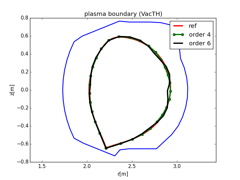
Figure 2: A WEST equilibrium case. The reference plasma boundary from the equilibrium code CEDRES++ and the boundary reconstructed using harmonics of order 4 in VacTH (bullets) are almost superimposed. The boundary reconstructed using harmonics of order 6 presents some unrealistic oscillations.

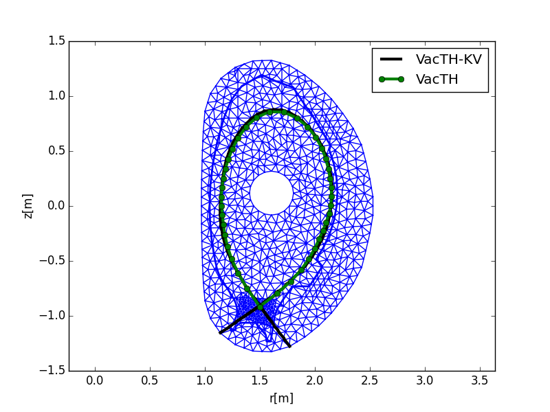
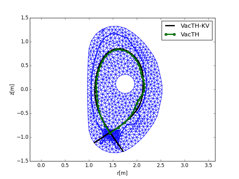
Figure 3: AUG shot 25374 plasma boundary reconstructions at time $1.1$s (top) and time $2.5$ (bottom). The plasma boundary computed from toroidal harmonics of order 4 in VacTH (bullets) is satisfatory at $1.1$s but presents unrealistic oscillations at $2.5$s. The plasma boundaries computed with the new proposed method VacTH-KV are shown with continuous lines.

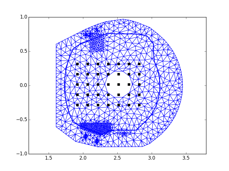
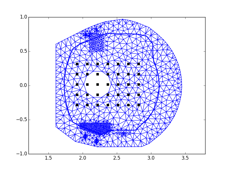
Figure 4: Examples of precomputed meshes for WEST. The limiter is represented. The mesh is refined in lower and upper X-point regions. Each small square inside the limiter region is the center of a circle defining an internal contour $\Gamma_{I}$.

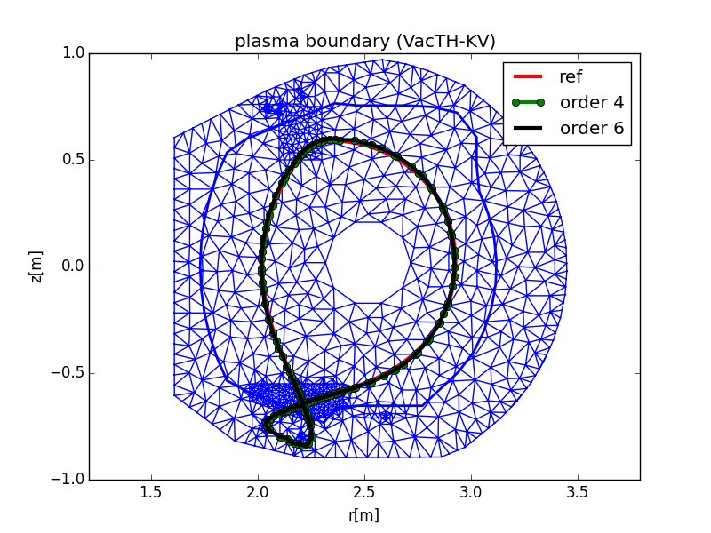
Figure 5: Same WEST test case as in Figure 2. The boundaries reconstructed with the new optimal control proposed method, VacTH-KV, using toroidal harmonics of order either 4 or 6 are almost superimposed with the reference boundary from CEDRES++

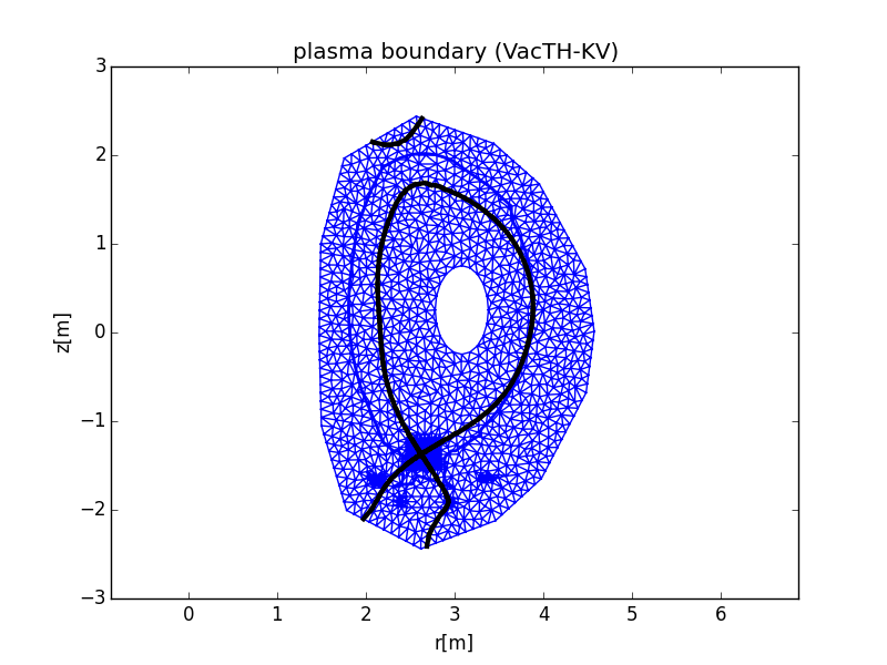
Figure 6: VacTH-KV boundary reconstruction for a JET test case example (shot 74221 at 46s). The method using toroidal harmonics only, VacTH, could not reconstruct a proper boundary.

References

- 1. J. WESSON, Tokamaks, volume 118 of International Series of Monographs on Physics, Oxford University Press Inc., New York (Third Edition, 2004).
- 2. D. LEE and Y.-K. M. PENG, “An approach to rapid plasma shape diagnostics in Tokamaks,” J. Plasma Phys., 25, 161 (1981).
- 3. G. DESHKO, T. KILOVATAYA, Y. KUZNETSOV, V. PYATOV, and I. YASIN, “Determination of the plasma column shape in a Tokamak from magnetic measurements,” Nuc. Fus., 23, 10, 1309 (1983).
- 4. S. BONDARENKO et al., “Measurement of the shape of the plasma column in the Tuman-3 Tokamak,” Sov. J. Plasma Phys., 10, 520 (1984).
- 5. F. ALLADIO and F. CRISANTI, “Analysis of MHD Equilibria by toroidal multipolar expansions,” Nuc. Fus., 26, 9, 1143 (1986).
- 6. K. KURIHARA, “Improvement of Tokamak plasma shape identification with a Legendre-Fourier expansion of the vacuum poloidal flux function,” Fusion Tech., 22, 334 (1992).
- 7. B. VAN MILLIGEN and A. LOPEZ FRAGUAS, “Expansion of vacuum magnetic fields in toroidal harmonics,” Comput. Phys. Comm., 81, 74 (1994).
- 8. Y. FISCHER, Approximation dans des classes de fonctions analytiques généralisées et résolution de problèmes inverses pour les tokamaks, Phd thesis, Université de Nice Sophia Antipolis, France, 2011.
- 9. B. FAUGERAS, J. BLUM, C. BOULBE, P. MOREAU, and E. NARDON, “2D interpolation and extrapolation of discrete magnetic measurements with toroidal harmonics for equilibrium reconstruction in a Tokamak,” Plasma Phys. Control. Fusion, 56, 114010 (2014).
- 10. B. BRAAMS, “The interpretation of Tokamak magnetic diagnostics,” Plasma Phys. Control. Fusion, 33, 7, 715 (1991).
- 11. J. BUCALOSSI et al., “Feasibility study of an actively cooled tungsten divertor in Tore Supra for {ITER} technology testing,” Fus. Engin. Des., 86, 6–8, 684 (2011), Proceedings of the 26th Symposium of Fusion Technology (SOFT-26).
- 12. H. HEUMANN et al., “Quasi-static free-boundary equilibrium of toroidal plasma with CEDRES++: computational methods and applications,” J. Plasma Phys. (2015).
- 13. R. KOHN and M. VOGELIUS, “Determining conductivity by boundary measurements: II. Interior results,” Commun. Pure Appl. Math., 31, 643 (1985).
- 14. B. FAUGERAS, A. BEN ABDA, J. BLUM, and C. BOULBE, “Minimization of an energy error functional to solve a Cauchy problem arising in plasma physics: the reconstruction of the magnetic flux in the vacuum surrounding the plasma in a Tokamak,” ARIMA, 15, 37 (2012).
- 15. J. BLUM, “Identification of free boundaries and non-linearities for elliptic partial differential equations arising from plasma physics,” Proc. Proceedings of the IFIP WG 7.2 Working Conference. Lecture Notes in Control and Information Sciences. Control of Partial Differential Equations, p. 11–22, Santiago de Compostela, Spain, july, 1987.
- 16. J. BLUM, Numerical Simulation and Optimal Control in Plasma Physics with Applications to Tokamaks, Series in Modern Applied Mathematics, Wiley Gauthier-Villars, Paris (1989).
- 17. W. FENEBERG, K. LACKNER, and P. MARTIN, “Fast control of the plasma surface,” Comput. Phys. Comm., 31, 2, 143 (1984).
- 18. S. HAKKARAINEN and J. FREIDBERG, “Reconstruction of vacuum flux surfaces from diagnostic measurements in a tokamak,” Massachussetts Institute of Technology, Report PFC/RR-87-22 (1987).
- 19. K. KURIHARA, “Tokamak plasma shape identification on the basis of boundary integral equations,” Nuc. Fus., 33, 3, 399 (1993).
- 20. K. KURIHARA, “A new shape reproduction method based on the Cauchy-condition surface fro real-time tokamak reactor control,” Fus. Engin. Des., 51-52, 1049 (2000).
- 21. B. BRAAMS, Computational studies in Tokamak equilibrium and transport, PhD thesis, University of Utrecht, 1986.
- 22. R. COURANT and D. HILBERT, Methods of Mathematical Physics, volume 1-2, Interscience (1962).
- 23. V. SHAFRANOV and L. ZAKHAROV, “Use of the virtual-casing principle in calculating the containing magnetic field in toroidal plasma systems,” Nuc. Fus., 12, 599 (1972).
- 24. J. SEGURA and A. GIL, “Evaluation of toroidal harmonics,” Comput. Phys. Comm., 124, 104 (2000).
- 25. L. ZAKHAROV and V. SHAFRANOV, “Equilibrium of a Toroidal Plasma with Non-circular Cross Section,” Sov. Phys. Tech. Phys., 18, 151 (1973).
- 26. ITM, “Integrated Tokamak Modelling,” http://portal.efda-itm.eu/, 2013.
- 27. P. CIARLET, The Finite Element Method For Elliptic Problems, North-Holland (1980).
- 28. C. HANSEN, Rank-Deficient and Discrete Ill-Posed Problems: Numerical Aspects of Linear Inversion, SIAM, Philadelphia (1998).
- 29. F. ZAITSEV, Mathematical modeling of toroidal plasma evolution, English edition. - M.:MAKS Press (2014).