Fluid friction and wall viscosity of the 1D blood flow model

Abstract

We study the behavior of the pulse waves of water into a flexible tube for application to blood flow simulations. In pulse waves both fluid friction and wall viscosity are damping factors, and difficult to evaluate separately. In this paper, the coefficients of fluid friction and wall viscosity are estimated by fitting a nonlinear 1D flow model to experimental data. In the experimental setup, a distensible tube is connected to a piston pump at one end and closed at another end. The pressure and wall displacements are measured simultaneously. A good agreement between model predictions and experiments was achieved. For amplitude decrease, the effect of wall viscosity on the pulse wave has been shown as important as that of fluid viscosity.

Keywords: Pulse wave propagation; One-dimensional modeling; Fluid friction; Viscoelasticity

1 Introduction

Although the modeling of blood flow has a long history, it is still a challenging problem. Recently 1D modeling of blood flow circulation has attracted more attention. One reason is that it is a well balanced option between complexity and computational cost (see e.g. [2, 7, 17, 21, 26, 30]). It is not only very important to predict the time-dependent distributions of flow rate and pressure in a network, but it is also important to be able to predict mechanical properties of the wall (see [14]), it is clear that could help the underestanding of cardiovascular pathologies.

The 1D fluid dynamical models are non nonlinear and are able to predict flow, area and pressure. Within the dynamical system there exist several damping factors, such as the fluid viscosity, the wall viscoelasticity, the geometrical changes of vessels, etc. Previous studies have shown that in vessels without drastic geometrical variations (i.e. no severe aneurysms or stenoses), the fluid viscosity and wall viscoelasticity are the most significant damping factors [16]. Comparisons between the 1D model and in-vivo data [11, 22] suggest that the predictions of a viscoelastic 1D model is significantly more physiological than those of an elastic one which contains high frequencies in the pulse which is not observed experimentally. But the comparisons were only qualitative or semi-quantitative due to the limited accuracy of associated non-invasive measurements and the lack of patient-specific parameter values of the 1D model for each subject.

Quantitative comparisons can be done with in-vitro experimental setups. Reuderink et al. [20] connected a distensible tube to a piston pump, which ejects fluid in pulse waves throughout the tube, and the experimental data were compared against numerical predictions of several formulations of the 1D model. In the first formulation, they proposed an elastic tube law and Poiseuille’s theory to account for the fluid viscosity, and their studies underestimated the damping of the waves and predicted shocks, not observed in the experiments. In another formulation, still linear, the fluid viscosity was predicted from the Womersley theory with a viscoelastic tube law which gave a better match between the predictions and the experiments. A similar experiments setup was proposed by Bessems et al. [5] using a 3-component Kelvin viscoelastic model to model the wall behavior, however in this work, both the convective and fluid viscosity terms were neglected. Alastruey et al. [1] presented a comparative study using an experimental setup with a network, they measured the coefficients of a Voigt viscoelastic model by tensile tests instead of fitting them from the waves. For the fluid viscosity term, they adopted a value from literature, which was fitted from waves of coronary blood flow with an elastic wall model [24].

In this paper, we study the friction and wall viscoelasticity using the 1D model and a similar experimental setup where pulse waves are propagating in one distensible tube. However, there are three main differences between our study and previous ones:

1. Both of the two damping factors (fluid friction and wall viscosity) are modelled. Although there are several theories to estimate the friction term (see, e.g. [6, 13, 18]), the value is rarely determined experimentally besides the study of Smith et al. with an elastic model [24]. It is well known that fluid viscosity and wall viscoelasticity have damping influences on the pulse waves. These slight differences are discussed in [27], nevertheless it is difficult to evaluate them separately from pulse waves. However, the viscoelasticity has smoothing effect on the waveforms whereas the fluid friction does not [3], we investigated this claim by only accounting for the amplitude or the sharpness of the signal. The study shows the results of including both effects, one, or the other.

2. The viscoelasticity of the wall is measured in a new manner. The viscoelasticity of a solid material is difficult to measure accurately, even in an in-vitro setup. In our study, the viscoelasticity is determined through the pressure-wall perturbation relation of the vessel under operating conditions. The internal pressure is measured by a pressure sensor and the perturbation of the wall is measured by a Laser Doppler Velocimetry (LDV).

3. A shock-capturing scheme is applied as the numerical solver. In a nonlinear hyperbolic system, shocks may arise even if the initial condition is smooth (even for small viscoelasticity values). The Monotonic Upstream Scheme for Conservation Laws (MUSCL) scheme is able to capture shocks without non-physical oscillations, and is applied to discretize the governing equations and compared to the MacCormack scheme.

2 Methodology

2.1 One-dimensional model

We use the 1D governing equations for flows passing through an elastic cylinder of radius $R$ expressed in the dynamical variables of flow rate $Q$, cross-sectional area $A=2\pi R$ and internal average pressure $P$. The 1D equations can be derived by the integration over a cross-sectional area of the axy-symmetric Navier-Stokes equations of an incompressible fluid at constant viscosity, giving the following mass and momentum 1D conservation equations

$$\frac{\partial A}{\partial t}+\frac{\partial Q}{\partial x}=0,$$ (1)

$$\frac{\partial Q}{\partial t}+\frac{\partial}{\partial x}(\alpha\frac{Q^{2}}{A})+\frac{A}{\rho}\frac{\partial P}{\partial x}=-2\pi\nu\left[\frac{\partial v_{x}}{\partial r}\right]_{r=R},$$ (2)

where $v_{x}$ is the axial velocity, $\rho$ is the fluid density and $\nu$ is the kinematic viscosity of the fluid. The parameter $\alpha$ and the last term, the viscous or drag friction, depend on the velocity profile. In general, the axial velocity is also function of the radius coordinate $r$, v.i.z. $v_{x}=v_{x}(r,x,t)$. If we assume the profile has the same shape $\Psi(r)$ in every vessel cross-section along the axial direction, the velocity function can be separated as $v_{x}=U(x,t)\Psi(r)$, being $U$ the average velocity. If $\Psi(r)$ is known, the parameter $\alpha$ and the derivative $\frac{\partial v_{x}}{\partial r}$ that appears in the friction term can be therefore calculated. The friction drag can be approximated by $-C_{f}Q/A$. The radial profile $\Psi(r)$ is strongly dependent on the Womersley number defined by $R\sqrt{\omega/\nu}$, where the quantity $\omega$ is the angular frequency which characterizes the flow. If $\omega$ and $\nu$ are approximately constant, only the radius $R$ influences $\alpha$ and $C_{f}$, whose values should be determined by experiments for vessels with various diameters. When the transient inertial force is large, the profile is essentially flat, $\alpha=1$ [24]. With a thin viscous boundary layer, the inviscid core and a no-slip boundary condition, the friction term can be estimated (see e.g. [6, 18]). When the transient inertial force is small, the profile is parabolic, $\alpha=4/3$; the viscosity force is then dominating and $C_{f}=8\pi\nu$. Using the power law profile proposed by Hughes and Lubliner [12], Smith et al. [24] compute from coronary blood flow, $C_{f}=22\pi\nu$ and $\alpha=1.1$. This value of $C_{f}$ is used on other numerical works [1, 15] but setting $\alpha=1$ for simplification.

The viscoelasticity of the wall can be described using different viscoelastic models, e.g. [11, 22, 25] with displaying disctint numerical problems [19, 25]. In this study we use the two-component Voigt model, which relates the strain $\epsilon$ and stress $\sigma$ in the equation

$$\sigma=E\epsilon+\phi\frac{d\epsilon}{dt},$$ (3)

where $E$ is the Young’s modulus and $\phi$ is a coefficient for the viscosity. In reference [23, 28] we have shown that the model (i) fits experimental data and (ii) it is able to filter high frequencies.

For a tube with a thin wall, the circumferential strain $\epsilon_{\theta\theta}$ can be expressed as

$$\epsilon_{\theta\theta}=\frac{R-R_{0}}{(1-\eta^{2})R_{0}},$$ (4)

where $R_{0}$ is the reference radius without loading and $\eta$ is the Poisson ratio, which is 0.5 for an incompressible material. By Laplace’s law, the transmural difference between the internal pressure $P$ and the external pressure $P_{ext}$ is balanced with the circumferential stress $\sigma_{\theta\theta}$ in the relation

$$P-P_{ext}=\frac{h\sigma_{\theta\theta}}{\pi R}.$$ (5)

Combining Eq. 3, 4 and 5, we get

$$P-P_{exp}=\nu_{e}(R-R_{0})+\nu_{s}\frac{dR}{dt},$$ (6)

with

$$\nu_{e}=\frac{Eh}{(1-\eta^{2})A_{0}}\text{, and }\nu_{s}=\frac{\phi h}{(1-\eta^{2})A_{0}}.$$

Note that the radius $R$ in the denominators of the two coefficients is approximated by $R_{0}$ under the assumption that the perturbations are small.

If we assume $P_{ext}$ constant and inserting Eq. 6 into the 1D momentum equation to eliminate $P$, gives

$$\frac{\partial Q}{\partial t}+\frac{\partial}{\partial x}\bigl{(}\alpha\frac{Q^{2}}{A}+\frac{\beta}{3\rho}A^{\frac{3}{2}}\bigr{)}=-C_{f}\frac{Q}{A}+C_{v}\frac{\partial^{2}Q}{\partial^{2}x},$$ (7)

where

$$\beta=\frac{\sqrt{\pi}Eh}{(1-\eta^{2})A_{0}}\text{, and }C_{v}=\frac{\sqrt{\pi}\phi h}{2\rho(1-\eta^{2})\sqrt{A_{0}}}.$$

The 1D model was numerically solved by two approaches : MacCormack and MUSCL. More details on the integration schemes and on the treatment of the boundary condition are in [8, 27]. More precisely here the boundary condition modeling the stainless rod in the experiment, a total reflection boundary condition, can be numerically achieved by imposing a mirror condition at the end of the elastic tube.

2.2 Experimental setup

The experimental setup is shown in Fig. 1. The piston pump (TOMITA Engineering) injects fluid (water) into a polyurethane tube. Theoutput of the pump is a sinusoidal function in time, whose period and duration can be programmed through a computer. At the measurement points, a pressure sensor (Keyence, AP-10S) is inserted into the tube. The perturbation of the tube wall is measured by a LDV (Polytec, NLV-2500). The pump, the pressure sensor and the LDV are controlled by a computer, which synchronizes the operations of the instruments and stores the measurement data at 10 $KHz$. The end of the tube is closed by a stainless rod and thus a total reflection boundary condition is imposed at the outlet. Pulse waves are bounced backward and forward in the tube multiple times before the equilibrium state is restored. We measured at two points, $A$ and $B$, which are respectively close to the proximal and distal ends of the tube. Table 1 summarizes the parameters of the elastic tube and fluid: the thickness of the wall $h$, the reference diameter $D$, the total length of the tube $L$, the distances from the inlet to the two measurement points $L_{A}$ and $L_{B}$, the fluid density $\rho$ and the kinematic viscosity $\nu$.

$h\leavevmode\nobreak\ (\text{cm})$	$D\leavevmode\nobreak\ (\text{cm})$	$L\leavevmode\nobreak\ (\text{cm})$	$L_{A}\leavevmode\nobreak\ (\text{cm})$	$L_{B}\leavevmode\nobreak\ (\text{cm})$	$\rho\leavevmode\nobreak\ (\text{kg}/\text{cm}^{3})$	$\nu\leavevmode\nobreak\ (\text{cm}^{2}/\text{s})$
0.2	0.8	192	28.3	168.2	1.050$\times 10^{-3}$	1$\times 10^{-2}$

Table 1: Parameters of the tube and fluid.

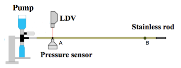
Figure 1: Experimental setup : the elastic tube (in yellow) is closed by a stainless rod at the right end (in grey). The points $A$ and $B$ indicate the measurement sites. Parameters of the tube and fluid are summarized in Table 1.

To evaluate independently the Young’s modulus of the elastic tubes we complete the experimental setup with a tensile device. We prepared two specimens of the polymer of the elastic wall to use in the tensile test (Shimadzu EZ test). The specimens were elongated at a rate of 0.5 $\text{m}/\text{min}$ and then released at the same rate. We applied the least square method (linear regression) to fit the curve against the function $F=C_{0}+ES\Delta L/L$, where $C_{0}$ is a constant, $E$ is the Young’s modulus, $S$ is the cross-sectional area of the specimens and $L$ is the original length. Dividing the fitted slope of the curve by $S$, we can estimate experimentally the Young’s modulus as 1.92$\pm$0.06 $10^{5}$ Pa.

Figure 2: Experimental pressure-radius (P-R) loop. Insert : one period loop. Note that the system in the linear regime.

2.3 Parameter estimation

We present the method used for the evaluation of the Young’s modulus, the wall viscosity and the fluid friction.

2.3.1 Young’s modulus

In order to estimate the Young’s modulus $E$ we propose two different methods: using numerical simulations and by integration of the experimental pressure-radius curve shown in Figure 2. We note that the system is in the linear zone. The values of $E$ computed in each approach will be compared to those given by the tensile test.

Numerical simulations

In the first approach, using the fact the velocity of pulse wave is directly related to the stiffness through the Moens-Korteweg formula [9], we vary Young’s modulus in numerical simulations to match the wave peaks coming from experimental signal taken in points $A$ and $B$. The best fit will give the optimal Young’s modulus $E_{0}$.

Integration of the experimental pressure-radius signal

In the second approach we use the experimental data and impose a sinusoidal wave of only one full period strictly. The net volume of fluid injected into the tube was zero, and the tube returned to the original state with the amplitude dampened roughly in a oscillatory way. In this situation the energy loss is due to the wall viscosity. Integrating the viscoelastic tube law (6) times the wall velocity $\frac{dR}{dt}$ from the starting time $t_{0}$ to the final time $t_{e}$ we found that the work done by the mechanical system is

$$\int_{t_{0}}^{t_{e}}(P-P_{ext})\frac{dR}{dt}\ dt=\int_{t_{0}}^{t_{e}}\nu_{e}(R-R_{0})\frac{dR}{dt}\ dt+\int_{t_{0}}^{t_{e}}\nu_{s}\left(\frac{dR}{dt}\right)^{2}\ dt.$$ (8)

From the time series of the pressure $P(t)$ and the wall displacement $R(t)$ the evaluation of the viscoelastic term $\nu_{s}$ is straightforward as long as both the external pressure $P_{ext}$ and the work done by the elastic component (the 1st term of the rhs of equation (8)) are zero. Once the viscosity coefficient $\nu_{s}$ is calculated, the tube law (6) can be rearranged to give $P-P_{ext}-\nu_{s}(dR/dt)=\nu_{e}(R-R_{0})$ and the elastic coefficient $\nu_{e}$ can be estimated by linear regression. We note that we have additionally estimated the viscoelastic term.

2.3.2 Viscoelastic parameters

For the estimation of the viscoelasticity parameters, we introduce a cost function defined by the normalized root mean square (NRMS) error between the experimental signal of pressure $P_{exp}$ and the numerical predictions $P_{sim}$

$$NRMS=\frac{1}{\max({P_{exp}})-\min({P_{exp}})}\sqrt{\frac{\sum_{N}({P_{sim}-P_{exp}})^{2}}{N}},$$

where $N$ is the number of temporal data points and $P_{sim}$ depends on the fluid friction and wall viscosity for fixed Young’s modulus $E_{0}$. For each run we obtain numerically the temporal series of the cross-sectional area $A$ from equation (1) and compute the numerical prediction of the pressure using equation (6). In practice, we fixed $C_{f}$ for different values from $8\pi\nu$ to $33\pi\nu$, and for each value, we fitted the parameters $\phi$ by minimizing the NRMS. As $C_{f}$ was fixed for each step we only did an one dimensional minimization by doing small variations of $\phi$ to find the minimum. This is particular case of the Steepest Descent approach for a functional minimum, where the new search direction is orthogonal to the previous. The parameter optimisation was done on the two measurement points $A$ and $B$, and the consistency of the results estimated from the two sets of data was checked.

3 Results

In this Section we present the results of the parameter estimations using the methods described before. Please note that the final state on the experimental data as well as the numerical results has a higher pressure than the initial state. That is because we imposed a half sinusoidal wave at the inlet and thus a net volume of about 4.5 $\text{cm}^{3}$ fluid was injected into the tube. Only in the case when we do the integration of the experimental pressure-radius signal to computed the wall viscosity and the fluid friction we impose a complete period at the inlet in order of to have no net extra volume inside the elastic tube.

3.1 Young’s modulus

We vary Young’s modulus $E$ in different simulations imposing a half sinusoidal wave at the inlet. Numerical simulations were done for $E$ starting from $2.00\times 10^{5}$ Pa to $2.15\times 10^{5}$ Pa, with a step of $0.01\times 10^{5}$ Pa. We have found that for the value of $E\sim E_{0}=2.08\times 10^{5}$ Pa, the difference of the arrival times between the experimental signal and predictions at the measurements points $A$ and $B$ was minimal (smaller than 0.02  s for each of the first ten peaks). The Figure 5 shows the variations of the arrival times when we change the Young’s modulus.

method	$E\leavevmode\nobreak\ (10^{5}\leavevmode\nobreak\ \text{Pa})$	$\phi\leavevmode\nobreak\ (\text{kPa}\cdot\text{s})$
Numerical	2.08	1.0
Integration P-R data	1.45—2.90	0.97—1.94
Tensile test	1.92$\pm$0.06	-

Table 2: Young’s modulus and Viscoelasticity of the polymer computed using three different approaches : 1D model optimisation, Pressure-radius experimental data and tensile test.

This value is in the range estimated with the integrated method $[1.45-2.9\ 10^{5}]$ and is about $8\%$ bigger than those give by the tensile device (1.92$\pm$0.06 $10^{5}$). Besides the measurement error, the variance in the home-made polymer tubes may also contribute to the difference.

3.2 Fluid friction and wall viscosity

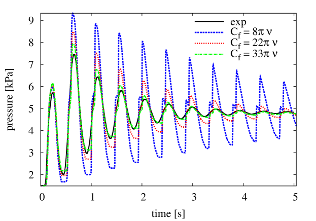
Figure 3: Pressure time series at measurement point A. The elastic model predicts shocks. Increasing the friction term can damp the amplitude effectively, but the shocks still exist. $E=2.08\times 10^{5}$ Pa and $\phi=0$.

The friction and wall viscosity terms are both damping factors in the model equation. The key point is to be able of discriminate them when we are looking for the optimal values.

First we used an pure elastic model (the wall viscosity $\phi$ is set to 0) and we varied the friction coefficient $C_{f}$. Fig. 3 presents the runs (called waves) with three values of the friction coefficient $C_{f}$: $8\pi\nu$, $22\pi\nu$ and $33\pi\nu$. Using the first value, derived from a parabolic velocity profile, the predicted pressure wave has two main unrealistic features: (i) we have an overestimated pressure amplitude and (ii) we develop discontinuities or shocks, in contradiction to the experimental measurement (blue line, Fig. 3). The second value comes from Smith et al. [24], and we can see the amplitude becomes closer to the experimental one (red line, Fig. 3). The third value gives the best prediction in terms of pressure amplitude but there are still discontinuities or shocks (green line, Fig. 3). We recall that, for a pure elastic model, we have always a finite time discontinuities, which is proper to the hyperbolic structure of the governing equations.

	wave1	wave2	wave3	wave4	wave5	wave6	wave7
$C_{f}(\pi\nu)$	8	14	18	22	26	30	33
$\phi(\text{kPa}\cdot\text{s})$	2.0	1.6	1.3	1.0	0.8	0.5	0.4
NRMS (%)	1.96	1.75	1.66	1.64	1.74	1.92	2.15

Table 3: Parameters of fluid friction and wall viscosity and the corresponding NRMS. Each wave correspond to a different run.

Table 3 summarizes the runs (wave 1 to 7) for different values of $C_{f}$, together with the optimal value of $\phi$ found by optimization and the corresponding residuals of NRMS. We observe for increasing values of $C_{f}$ increases that the parameter $\phi$ decreases. The minimal residual of NRMS achieves for wave4 and the limit cases (wave 1 and wave 7) are the worsts.

We plotted waves 1, 4 and 7 in Fig. 4. First we noticed that the discontinuities or shocks disappear and that the amplitude of the three waves are close to the experimental data. However, in the first two seconds of the temporal series, the wave-front of wave 7 is steeper than the others. This difference is more clear when we plot the power spectrum of the time series (Fig. 4), which shows that the high frequency components of wave 7 are underdamped. This is because the damping effect of wall viscosity is stronger on high frequency waves while that the fluid friction does not depend on the frequency in our model. In the last part of the time records, only the main harmonic is still present, thus the difference between the three simulated waves is very small. The viscoelastic parameters estimated by the presented methods are summarized in Table 2. The values estimated by the data fitting with the 1D model fall into the range measured by the integrated approach of the pressure-radius (P-R) series data.

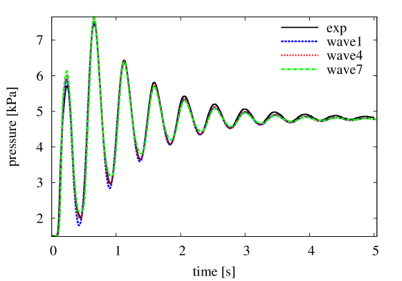
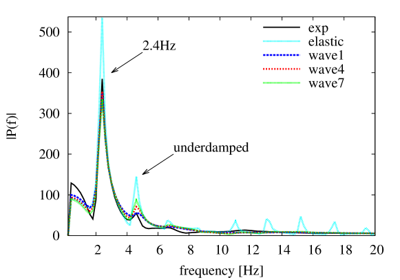
Figure 4: Experiments (line labelled exp) and simulations at measurement point $A$. Left (a): pressure time series. Right (b): spectrum of the pressure series (only frequencies less than 20 Hz are shown). $E=2.08\times 10^{5}$ Pa. For the elastic case, $C_{f}=22\pi\nu$ and $\phi=0$. The values of $C_{f}$ and $\phi$ for the three viscoelastic waves are shown in Table 3.

3.3 Sensitivity study

Fig. 5 presents the parameter sensitivity for Young’s modulus $E$ having a variance of 10% around $E_{0}$. The arrival time of each peak is significantly later when $E$ decreases and vice versa.

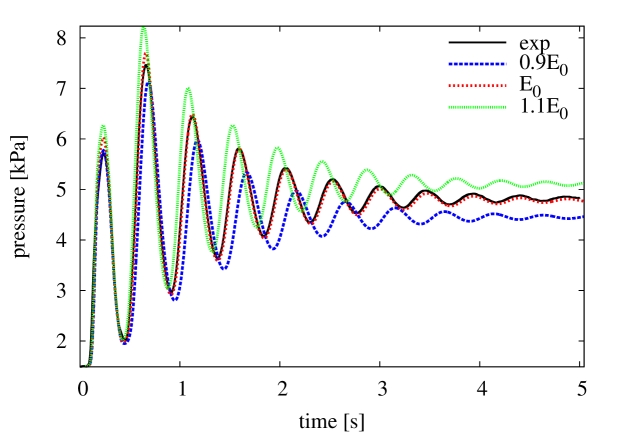
Figure 5: Sensitivity study. Pressure time series at measurement point A. $E_{0}$ is the best fit for the Young’s modulus. If $E_{0}$ is perturbed 10%, the arrival time of each peak changes significantly. $C_{f}=22\pi\nu$ and $\phi=0.9$ $\text{kPa}\cdot\text{s}$.

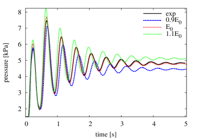
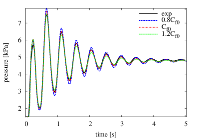
Figure 6: Time series of pressure with a 20% uncertainty of $C_{f}$ (left) and $\phi$ (right).

We also tested the sensitivity of the model to $C_{f}$, $\phi$ and $\alpha$. For $C_{f}$ and $\phi$, an uncertainty of about 20% produces a moderate variance on the predicted wave (see Fig. 6 and  6). The sensitivity of the output to $C_{f}$ and $\phi$ is in the same order. In contrast, when $\alpha$ is tested in the range from 1.0 to 1.3, there is no noticeable difference between the numerical predictions. Thus, the value of $\alpha$ can be set to 1.0. There exists indeed more sophisticated sensitivity techniques [29] but it is beyond the presented study.

3.4 Integration schemes

Measurement $A$	Measurement $B$

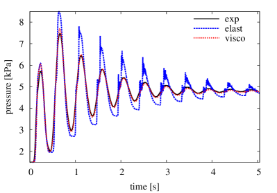
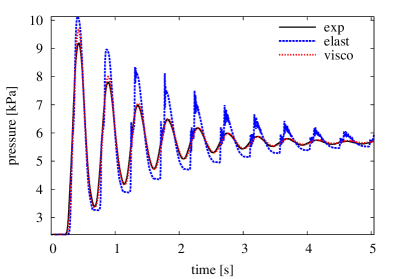
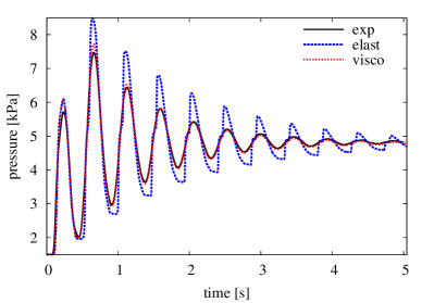
Figure 7: Pressure time series at the two measurement points with two numerical schemes. Left column: point $A$, right column: point $B$. Top row: MacCormack method, bottom row: MUSCL method. The viscoelastic model predicts much better than the elastic model at both the measurement points. The MUSCL method depresses the numerical oscillations when there are shocks. The parameters are: $E=2.08\times 10^{5}$ Pa, $C_{f}=22\pi\nu$, and $\phi$=1.0 $\text{kPa}\cdot\text{s}$ (visco).

We tested two different integration schemes : MacCormack and MUSCL. We compared the performances for a pure elastic as well as for a viscoelastic model. In Fig. 7, we plotted the pressure waves for the numerical predictions against the experiments data at the two measurement points: left column for point $A$ and right column for point $B$.

The discontinuities or shocks predicted by the elastic model are very obvious. The MacCormack scheme produces numerical oscillations (top row) whereas the MUSCL scheme depresses them because it includes a slope limiter (bottom row). For the viscoelastic model, the shocks disappear and a much better agreement is found at both locations $A$ and $B$. If the solution is quite smooth, there is essentially no difference between the two numerical schemes in accuracy. The consistency between the two locations make us confident in the agreement between experiments and numerical simulations.

4 Discussion

We evaluated the stiffness and friction within a nonlinear 1D fluid dynamical model with a viscoelastic law for the wall mechanics against experimental data.

The value of vessel stiffness estimated by the 1D model was compared to values measured using a tensile test. We notethat a small variance in stiffness can significantly the change the mean pressure, pulse pressure and wave velocity. Under the operating pressure within our experiment, the nonlinearity seems not large as shown in Figure 2. However, we note that the nonlinearity may be more significant under physiological conditions. More studies have to be done to evaluate the nonlinear elasticity of the arteries under real conditions.

The fluid friction and wall viscosity were fitted from experimental data using the 1D model. We obtained good agreement between the 1D model results and experiments. If experimental uncertainties are considered, it can be estimated that $C_{f}=22\pm 4\pi\nu$ and $\phi=1.0\pm 0.3\leavevmode\nobreak\ \text{kPa}\cdot\text{s}$ (determined by the runs wave3 and wave5 in Table 2). Our results confirm that in cases of blood flow with a similar characteristic Womersley number, the Poiseuille model underestimates the fluid friction (see e.g. [23]). The widely used value $C_{f}=22\pi\nu$ in large arteries is then acceptable. However, in smaller arteries, the Womersley number can be less than one, so a parabolic velocity profile is more likely to appear, which implies that $C_{f}$ decreases to $8\pi\nu$. Thus the friction term should vary through the whole cardiovascular system and a smaller value of $C_{f}$ should be considered if the Womersley number is smaller.

In our experimental study, the frequency of the main harmonic is 2.4 Hz (see Fig. 4) and thus the Womersley number is about 15.5. This value is only slightly bigger than the Womersley number at the ascending aorta which is 13.2 [10]. Under in vivo conditions, the wall viscosity is much larger as measured by Armentano et al. [4]. However the surrounding tissues of the vessel such as fat may also damp the waves attributed wall viscosity. The viscoelasticity of the arteries is mostly attributed to the collagen and elastin fibers in the wall, which is different from the polymer tube.

The viscoelasticity of the wall dampens the high frequency components of the wave, thus the waveform is not very front-steepened, which has been pointed out by many previous studies (see e.g. [1, 11]). A perturbation of 20% on wall viscosity introduces moderate variances on the pressure waveform, which is similar to the fluid friction (see Fig. 6 and  6). The output of the 1D model is not very sensitive to uncertainties of the two damping factors. Thus it is possible to use general values of those two parameters even in patient-specific simulations with the 1D model.

We solved the nonlinear 1D viscoelastic model with MacCormack and MUSCL schemes. The elastic model predicts shocks, which are captured by the MUSCL method without non-physical oscillations.

Some limitations of our approach are : while the flow rate may be similar, material properties are likely different and the in vivo (invasive) pressure measurements could hardly to including in a clinical protocol. One could advance that in real arteries under normal physiological conditions, discontinuities or shocks are not present but in pathologocal situations (anasthomoses, artheromes) or after surgeries (i.e. stent) the discontinuities on the Young’s modulus of the arterial wall can lead to flow discontinuities. Concerning the boundary conditions, arteries never display this type of vessel ending but it is not unreasonable to image a clinical protocol with a short stopping blood flow to observe localized backward waves.

5 Conclusion

We studied and evaluated the parameters of the nonlinear 1D viscoelastic model using data from an experimental setup. The 1D model was solved by two schemes, one of which is shock-capturing.

The value of vessel stiffness, estimated by the 1D model was consistent with values obtained by an integrated method using experimental data (pressure-radius time series) and tensile tests. The fluid friction and wall viscosity were fitted from data measured at two different locations. The estimated viscoelasticity parameters were consistent with values obtained with other methods. The good agreement between the predictions and the experiments indicate that the nonlinear 1D viscoelastic model can simulate the pulsatile blood flow very well. We showed that the effect of wall viscosity on the pulse wave is as important as that of fluid viscosity.

Conflict of interest

All the authors have been involved in the design of the study and the interpretation of the data and they concur with its content. There are no conflicts of interest between the authors of this paper and other external researchers or organizations that could have inappropriately influenced this work.

References

- [1] J. Alastruey, A.W. Khir, K.S. Matthys, P. Segers, S.J. Sherwin, P.R. Verdonck, K.H. Parker, and J. Peiró. Pulse wave propagation in a model human arterial network: Assessment of 1-d visco-elastic simulations against in vitro measurements. Journal of biomechanics, 44(12):2250–2258, 2011.
- [2] J. Alastruey, K.H. Parker, and S.J. Sherwin. Arterial pulse wave haemodynamics. In Proc. BHR Group’s 11th International Conference on Pressure Surges, Lisbon, Portugal, pages 401–443, 2012.
- [3] J. Alastruey, T. Passerini, L. Formaggia, and J. Peiró. Physical determining factors of the arterial pulse waveform: theoretical analysis and calculation using the 1-d formulation. Journal of Engineering Mathematics, 77(1):19–37, 2012.
- [4] R.L. Armentano, J.G. Barra, J. Levenson, A. Simon, and R.H. Pichel. Arterial wall mechanics in conscious dogs assessment of viscous, inertial, and elastic moduli to characterize aortic wall behavior. Circulation Research, 76(3):468–478, 1995.
- [5] D. Bessems, C.G. Giannopapa, M. Rutten, and F.N. van de Vosse. Experimental validation of a time-domain-based wave propagation model of blood flow in viscoelastic vessels. Journal of biomechanics, 41(2):284–291, 2008.
- [6] D. Bessems, M. Rutten, and F. Van De Vosse. A wave propagation model of blood flow in large vessels using an approximate velocity profile function. Journal of Fluid Mechanics, 580:145–168, 2007.
- [7] W. Cousins and P.-A. Gremaud. Boundary conditions for hemodynamics: The structured tree revisited. Journal of Computational Physics, 231(18):6086–6096, 2012.
- [8] O. Delestre and P.-Y. Lagrée. A ‘well-balanced’ finite volume scheme for blood flow simulations. International Journal for Numerical Methods in Fluids, 72(2):177–205, 2013.
- [9] L. Formaggia, D. Lamponi, and A. Quarteroni. One-dimensional models for blood flow in arteries. Journal of Engineering Mathematics, 47:251–276, 2003.
- [10] Y.C. Fung. Biomechanics: circulation. Springer Verlag, New York, US, 1997.
- [11] R. Holenstein, P. Niederer, and M. Anliker. A viscoelastic model for use in predicting arterial pulse waves. Journal of biomechanical engineering, 102(4):318–325, 1980.
- [12] T.J.R. Hughes and J. Lubliner. On the one-dimensional theory of blood flow in the larger vessels. Mathematical Biosciences, 18(1):161–170, 1973.
- [13] P.-Y. Lagrée. An inverse technique to deduce the elasticity of a large artery. EPJ Applied Physics, 9(2):153–164, 2000.
- [14] D. Lombardi. Inverse problems in 1d hemodynamics on systemic networks: A sequential approach. International journal for numerical methods in biomedical engineering, 30(2):160–179, 2014.
- [15] E. Marchandise, M. Willemet, and V. Lacroix. A numerical hemodynamic tool for predictive vascular surgery. Medical Engineering and Physics, 31(1):131–144, 2009.
- [16] K.S. Matthys, J. Alastruey, J. Peiró, A.W. Khir, P. Segers, P.R. Verdonck, K.H. Parker, and S.J. Sherwin. Pulse wave propagation in a model human arterial network: Assessment of 1-d numerical simulations against in vitro measurements. Journal of Biomechanics, 40(15):3476–3486, 2007.
- [17] M.S. Olufsen, N.A. Hill, G.D.A. Vaughan, C. Sainsbury, and M. Johnson. Rarefaction and blood pressure in systemic and pulmonary arteries. Journal of fluid mechanics, 705:280–305, 2012.
- [18] M.S. Olufsen, C.S. Peskin, W.Y. Kim, E.M. Pedersen, A. Nadim, and J. Larsen. Numerical simulation and experimental validation of blood flow in arteries with structured-tree outflow conditions. Annals of Biomedical Engineering, 28(11):1281–1299, 2000.
- [19] R. Raghu, I.E. Vignon-Clementel, C.A. Figueroa, and C.A. Taylor. Comparative study of viscoelastic arterial wall models in nonlinear one-dimensional finite element simulations of blood flow. Journal of biomechanical engineering, 133(8):081003, 2011.
- [20] P.J. Reuderink, H.W. Hoogstraten, P. Sipkema, B. Hillen, and N. Westerhof. Linear and nonlinear one-dimensional models of pulse wave transmission at high womersley numbers. Journal of biomechanics, 22(8):819–827, 1989.
- [21] P. Reymond, P. Crosetto, S. Deparis, A. Quarteroni, and N. Stergiopulos. Physiological simulation of blood flow in the aorta: comparison of hemodynamic indices as predicted by 3-d fsi, 3-d rigid wall and 1-d models. Medical engineering & physics, 35(6):784–791, 2013.
- [22] P. Reymond, F. Merenda, F. Perren, D. Rüfenacht, and N. Stergiopulos. Validation of a one-dimensional model of the systemic arterial tree. American Journal of Physiology-Heart and Circulatory Physiology, 297(1):H208–H222, 2009.
- [23] M. Saito, Y. Ikenaga, M. Matsukawa, Y. Watanabe, T. Asada, and P.-Y. Lagrée. One-dimensional model for propagation of a pressure wave in a model of the human arterial network: Comparison of theoretical and experimental results. Journal of Biomechanical Engineering, 133:121005, 2011.
- [24] N.P. Smith, A.J. Pullan, and P.J. Hunter. An anatomically based model of transient coronary blood flow in the heart. SIAM Journal on Applied mathematics, 62(3):990–1018, 2002.
- [25] B.N. Steele, D. Valdez-Jasso, M.A. Haider, and M.S. Olufsen. Predicting arterial flow and pressure dynamics using a 1d fluid dynamics model with a viscoelastic wall. SIAM Journal on Applied Mathematics, 71(4):1123–1143, 2011.
- [26] F.N. van de Vosse and N. Stergiopulos. Pulse wave propagation in the arterial tree. Annual Review of Fluid Mechanics, 43(1), 2011.
- [27] X. Wang, J.-M. Fullana, and P.-Y. Lagrée. Verification and comparison of four numerical schemes for a 1d viscoelastic blood flow model. Computer Methods in Biomechanics and Biomedical Engineering, 18 (15), 2014.
- [28] X.-F. Wang, J.-M. Fullana, P.-Y. Lagrée, and R.L. Armentano. Effect of viscoelasticity of arterial wall on pulse wave: a comparative study on ovine. Computer methods in biomechanics and biomedical engineering, 16(sup1):25–26, 2013.
- [29] D. Xiu and S.J. Sherwin. Parametric uncertainty analysis of pulse wave propagation in a model of a human arterial network. Journal of Computational Physics, 226(2):1385–1407, 2007.
- [30] Y. Yamamoto, M. Saito, Y. Ikenaga, M. Matsukawa, Y. Watanabe, M. Furuya, and T. Asada. Experimental study on the pulse wave propagation in a human artery model. Japanese Journal of Applied Physics, 50(7), 2011.