Goos-Hänchen Shifts in AA-Stacked Bilayer Graphene Superlattices

Youness Zahidi^a, Ilham Redouani^a and Ahmed Jellal^a,b

^aTheoretical Physics Group, Faculty of Sciences, Chouaïb Doukkali University,

PO Box 20, 24000 El Jadida, Morocco

^bSaudi Center for Theoretical Physics, Dhahran, Saudi Arabia

The quantum Goos-Hänchen shifts of the transmitted electron beam through an AA-stacked bilayer graphene superlattices is investigated. We found that the band structures of graphene superlattices can have more than one Dirac point, their locations do not depend on the number of barriers. It was revealed that any $n$-barrier structure is perfectly transparent at normal incidence around the Dirac points created in the superlattices. We showed that the Goos-Hänchen shifts display sharp peaks inside the transmission gap around two Dirac points ($E=V_{B}+\tau$, $E=V_{W}+\tau$), which are equal to those of transmission resonances. The obtained Goos-Hänchen shifts are exhibiting negative as well as positive behaviors and strongly depending on the location of Dirac points. It is observed that the maximum absolute values of the shifts increase as long as the number of barriers is increased. Our analysis is done by considering four cases: single, double barriers, superlattices without and with defect.

PACS numbers: 73.22.Pr, 72.80.Vp, 71.10.Pm, 03.65.Pm
Keywords: AA-stacked bilayer graphene, barriers, superlattices, transmission, Goos-Hänchen shifts.

1 Introduction

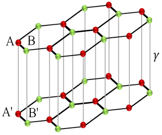
Figure 2: Schematic illustration of lattice structure of AA-stacked bilayer graphene, which consists of two graphene layers. Each carbon atom of the upper layer is located above the corresponding atom of the lower layer and they are separated by an interlayer coupling energy $\gamma$. The unit cell of the AA-stacked bilayer graphene consists of four atoms A, B, A’ and B’.

Since the first experimental fabrication of monolayer graphene [1], a single sheet of carbon honeycomb, it inspired researchers due to its unique electronic properties. This new material has a number of interesting properties, which makes it one of the most promising materials for future nanoelectronics [2]. What makes graphene so attractive is its band structure, which is gapless and exhibits a linear dispersion relation at two inequivalent points ($K$, $K^{\prime}$) in the vicinity of the Fermi energy. Moreover, its low energy of electrons is governed by a (2+1) dimensional Dirac equation, witch leads to many fascinating physical properties, such as Klein tunneling [3]. Graphene can not only exist in the free state, but two or more layers can stack above each other to form what is called few layer graphene, as the case for bilayer graphene (BLG), two stacked sheets. There are two dominant ways in which the two layers can be stacked to form AB or AA, with A and B are two sublattices of each layer, see Figure 2 for AA.

Owing to the interlayer interactions between the two layers and stacking sequence, the energy bands of AA-stacked BLG differ from those of the monolayer graphene and AB-stacked BLG. There are two pairs of linear bands intersecting at the Fermi level, that are a double copies of single layer graphene bands shifted up and down by the interlayer coupling $\gamma\approx 0.2\ eV$ [4]. Due to this special band structure, the AA-stacked BLG shows many interesting properties [4, 5, 6, 7, 8, 9] that are different from those of others. The research was less focused on AA-stacked BLG then AB-stacked BLG because of its instability, but actually recent experiment proved that one can produce a stable AA system  [10, 11, 12].

On the other hand, the Goos-Hänchen (GH) shift [13] is a phenomenon that originated in classical optics in which a light beam reflecting off a surface is spatially shifted as if it had briefly penetrated the surface before bouncing back. The GH shift was discovered by Hermann Fritz Gustav Goos and Hilda Hänchen [13, 14] and theoretically explained by Artman [15] in the late of 1940s. Usually, the absorption and transmission of the two optical materials must be weak enough to allow a reflected beam to be formed. Since its discovery, the beam spatial shift at total reflection suspected by Newton’s corpuscular theory has been extended to other fields of physics, such as quantum mechanics, plasma physics, acoustics [16], metamaterial [17], neutron physics [18] and graphene [19, 20, 21]. The Quantum version of the GH shifts is an analogue to the optical GH one, which is referred to a lateral shift between the reflected and incident beams occurring at the interface of two different materials on total internal reflection. Generally, its magnitude is in order of the Fermi wavelength.

Recently, interesting results were reported on the quantum GH shift for charge carriers in graphene systems [20, 21, 22, 23]. This does not only reflects the unique transport properties of Dirac electrons and holes in graphene nanostructures, but also promotes the application of graphene nanostructure in nanoelectronic devices. Motivated by recent experiments on graphene superlattices (SLs) [24, 25, 26], we consider a system of Dirac fermions through a periodic potential in graphene. We analyze the GH shifts of the transmitted electron beam scattered by the potential profile presented in Figure 1 through AA-staked BLG. After formulating our model we compute the associated energy eigenvalues and energy bands. We found that the energy bands are just the double copies of single layer graphene bands shifted up and down by the interlayer coupling $\gamma$. In addition, the bounds structure of graphene SLs can have more than one Dirac points, those locations do not depend on the number of barriers. Then, we used the transfer matrix method to determine the GH shifts and associated transmission probability. The numerical results show that the manifestation of Klein tunneling occur at normal incidence. Subsequently, we found that the GH shifts display sharp peaks inside the transmission gap around the two Dirac points ($E=V_{B}+\tau$, $E=V_{W}+\tau$), where the number of this peaks is equal to that of transmission resonances. Our findings are compared to those of single, double barrier structures and graphene SLs with a defect.

This paper is organized as follows. In section 2, we consider Dirac fermions in AA-stacked BLG system scattered by barrier potential (Figure 1). In section 3, we obtain the spinor solution corresponding to each regions composing our system. We use the transfer matrix at boundaries together with the incident, transmitted and reflected currents to end up with two transmission probabilities. In section 4, we numerically present our results for the GH shifts and the transmission probability of an electron beam transmitted through graphene SLs. Comparison with other graphene systems will done and the influence of the defect mode on our graphene SLs will be analyzed. We conclude our work and emphasize our main results in final section.

2 Theoretical model

We consider an AA-stacked BLG graphene SLs (graphene under periodic potential) with rectangular barriers grown along the x-direction. The potential profile is shown in Figure 1, where the symbols $"B"$, $"W"$ and $"D"$ denotes the barrier, well and the defect, respectively. The structure are characterized by the potential barrier height $V_{B}$ with gaps $\Delta_{B}$ and width $d_{B}$, the potential well height $V_{W}$ with gaps $\Delta_{W}$ and width $d_{W}$. The defect is denoted by the potential height $V_{D}$ with gaps $\Delta_{D}$ and width $d_{D}$. The incidence and transmission regions correspond to the gapless graphene with $\Delta=V=0$. Note that, similar potential profile have been recently considered in monolayer graphene in [22].

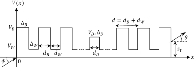
Figure 1: Schematic representation of the potential profile.

In the basis of $\psi=\left(\psi_{A},\ \psi_{B},\ \psi_{A^{{}^{\prime}}},\ \psi_{B^{{}^{\prime}}}\right)^{T}$, where $\psi_{A(A^{{}^{\prime}})}$ and $\psi_{B(B^{{}^{\prime}})}$ are the envelope functions associated with the probability amplitudes of the wave functions on the A(A${}^{{}^{\prime}}$) and B(B${}^{{}^{\prime}}$) sublattices of the upper (lower) layer, our system can be described by a single valley Hamiltonian

$$\mathcal{H}=\left(\begin{array}[]{cccc}V(x)+\Delta(x)&v_{F}(p_{x}-ip_{y})&\gamma&0\\ v_{F}(p_{x}+ip_{y})&V(x)-\Delta(x)&0&\gamma\\ \gamma&0&V(x)+\Delta(x)&v_{F}(p_{x}-ip_{y})\\ 0&\gamma&v_{F}(p_{x}+ip_{y})&V(x)-\Delta(x)\\ \end{array}\right)$$ (1)

where $p=(p_{x},p_{y})$ being the two-dimensional momentum operator, the Fermi velocity $v_{F}=10^{6}\ m/s$, the interlayer coupling $\gamma\approx 0.2\ eV$ [4], the gaps $\Delta(x)$ and potential $V(x)$. For graphene SLs with defect the potential is defined by

$$V(x)=\left\{\begin{array}[]{ccc}V_{B},&&\;\qquad nd\leq x\leq nd+d_{B}\\ V_{W},&&\;\qquad nd+d_{B}\leq x\leq(n+1)d\\ V_{D},&&\;\qquad Nd\leq x\leq Nd+d_{D}\end{array}\right.$$ (2)

and the gap reads as

$$\Delta(x)=\left\{\begin{array}[]{ccc}\Delta_{B},&&\;\qquad nd\leq x\leq nd+d_{B}\\ 0,&&\;\text{otherwise}\end{array}\right.$$ (3)

where $0\leq n\leq N-1$, $N$ being the number of period, such that the period is considered as the alternating barriers and wells with the width $d$ ($d=d_{B}+d_{W}$).

Due to the translation invariance in the y-direction, the momentum is a conserved quantity, then the eigenvalue of (1) takes the form

$$\psi(x,y)=e^{ik_{y}y}\psi(x,k_{y}).$$ (4)

Solving the eigenvalue equation $\mathcal{H}\psi=E\psi$, one finds the energy bands

$$\epsilon^{{\color[rgb]{1.00,0.00,0.00}s_{i}},\tau}_{i}=\tau+s_{i}\sqrt{\eta^{2}\left((k_{x_{i}}^{\tau})^{2}+(k_{y})^{2}\right)+\Delta_{i}^{2}}$$ (5)

where $\epsilon_{i}=E-V_{i}$, the index $i\ (i=B,\ W,\ D)$ corresponds to the barrier, well and defect regions,

$$k_{x_{i}}^{\tau}=\sqrt{-k_{y}^{2}+\eta^{-2}\left(\left(\epsilon_{i}-\tau\right)^{2}-\Delta_{i}^{2}\right)}$$ (6)

is the wave vector along the x-direction with $\tau$ is the cone index such that $\tau=+1$ ($\tau=-1$) for the upper (lower) cone and $s_{i}=\mbox{sign}(\epsilon_{i})$. We further introduce the length scale $\eta=\frac{\hbar v_{F}}{\gamma}\thickapprox 3.29~{}nm$ and switch to dimensionless quantities by measuring all energies terms in units of the interlayer coupling $\gamma$ such that $\epsilon_{i}\longrightarrow\frac{\epsilon_{i}}{\gamma}$, $\Delta_{i}\longrightarrow\frac{\Delta_{i}}{\gamma}$. For the incidence and transmission regions where we have $V=\Delta=0$, the energy bands are

$$E^{s_{0},\tau}=\tau+s_{0}\sqrt{\eta^{2}\left((k_{x_{0}}^{\tau})^{2}+(k_{y})^{2}\right)}$$ (7)

and the wave vector reads as

$$k_{x_{0}}^{\tau}=\sqrt{-k_{y}^{2}+\eta^{-2}\left(E-\tau\right)^{2}}$$ (8)

with $s_{0}=\mbox{sign}(E).$

Plots of the energy bands structure in AA-stacked BLG, evaluating (5) for the barrier region, have been shown in Figure 3. We clearly see that the energy bands are different from that of the AB-stacked BLG [27] and also monolayer graphene [1]. One can observe that for zero gap, the energy bands are linear and just two copies of the monolayer band structure shifted up and down by $\gamma=0.2\ eV$ (Figure 3(a)), respectively. In addition, the Dirac points are located at $E=V_{B}\pm\ \gamma$. For a finite gap, the spectrum is parabolic and the two Dirac points are lifted and they are shifted up and down by $\Delta_{B}$ (Figure 3(b)). We can observe that when the potential heights $V_{B}$ increase, the energy bands increase upwards.

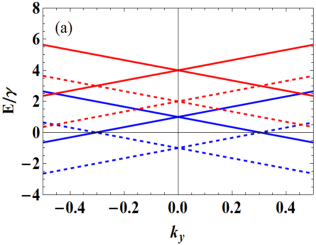
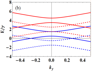
Figure 3: Energy bands as function of the momentum $k_{y}$. The solid and dashed curves correspond to the upper and lower cone i.e. $\tau=+1$ and $\tau=-1$, respectively, where the physical parameters are chosen to be, (a) : $V_{B}=0$ (blue curves), $V_{B}=3\gamma$ (red curves) and $\Delta_{B}=0$. (b) : $V_{B}=0$ (blue curves), $V_{B}=3\gamma$ (red curves) and $\Delta_{B}=0.5\gamma$.

As usual, to derive the eingespinors we solve $\mathcal{H}\psi=E\psi$. The corresponding eigenspinors can be written as

$$\psi_{i}=L_{i}\cdot A_{i}$$ (9)

where we have set

$$L_{i}=\left(\begin{array}[]{cccc}s_{i}f_{i}^{+,+}e^{ik_{x_{i}}^{+}x}&s_{i}f_{i}^{+,-}e^{-ik_{x_{i}}^{+}x}&s_{i}f_{i}^{-,+}e^{ik_{x_{i}}^{-}x}&s_{i}f_{i}^{-,-}e^{-ik_{x_{i}}^{-}x}\\ e^{ik_{x_{i}}^{+}x}&e^{-ik_{x_{i}}^{+}x}&e^{ik_{x_{i}}^{-}x}&e^{-ik_{x_{i}}^{-}x}\\ s_{i}f_{i}^{+,+}e^{ik_{x_{i}}^{+}x}&s_{i}f_{i}^{+,-}e^{-ik_{x_{i}}^{+}x}&-s_{i}f_{i}^{-,+}e^{ik_{x_{i}}^{-}x}&-s_{i}f_{i}^{-,-}e^{-ik_{x_{i}}^{-}x}\\ e^{ik_{x_{i}}^{+}x}&e^{-ik_{x_{i}}^{+}x}&-e^{ik_{x_{i}}^{-}x}&-e^{-ik_{x_{i}}^{-}x}\end{array}\right),\qquad A_{i}=\left(\begin{array}[]{cc}\alpha_{i}^{+}\\ \beta_{i}^{+}\\ \alpha_{i}^{-}\\ \beta_{i}^{-}\end{array}\right)$$ (10)

with

$$f_{i}^{\tau,\pm}=\pm\sqrt{\frac{E-V_{i}-\tau+\Delta_{i}}{E-V_{i}-\tau-\Delta_{i}}}e^{\mp i\phi_{i}^{\tau}},\qquad\phi_{i}^{\tau}=\arctan(k_{y}/k_{x_{i}}^{\tau}).$$ (11)

It may be noted that for AB-stacked BLG, in the four band model, we have four reflection and four transmission channels [27]. For AA-stacked BLG, all intercone transitions ($\tau\longrightarrow-\tau$) are strictly forbidden due to the orthogonality of electron wave functions with a different cone index [28], which yield to only two transmissions ($\tau\longrightarrow\tau$). Thus, we can reduce the $4\times 4$ matrix to the following $2\times 2$ matrix

$$L_{i}=\left(\begin{array}[]{cc}s_{i}\tau f_{i}^{\tau,+}e^{ik_{x_{i}}^{\tau}x}&s_{i}\tau f_{i}^{\tau,-}e^{-ik_{x_{i}}^{\tau}x}\\ \tau e^{ik_{x_{i}}^{\tau}x}&\tau e^{-ik_{x_{i}}^{\tau}x}\end{array}\right),\qquad A_{i}^{\tau}=\left(\begin{array}[]{cc}\alpha_{i}^{\tau}\\ \beta_{i}^{\tau}\\ \end{array}\right).$$ (12)

3 Transmission and Goos-Hänchen shifts

We are interested in the normalization coefficients, the components of $A_{i}^{\tau}$, on the both sides of the superlattices. In other words, for the incidence and transmission regions, we have, respectively

$$A_{in}^{\tau}=\left(1,r^{\tau}\right)^{T},\qquad A^{\tau}_{tr}=\left(t^{\tau},0\right)^{T}$$ (13)

where $r^{\tau}$ and $t^{\tau}$ are the reflection and transmission coefficients of each cone ($\tau=\pm 1$), respectively. The coefficients $r^{\tau}$ and $t^{\tau}$ are determined by imposing the continuity of the wave functions. For this, we need to match the wave functions at the boundaries between different regions. This procedure is most conveniently expressed in the transfer matrix formalism [29]. From the continuity of the wave function, we end up with

$$\left(\begin{array}[]{c}{1}\\ {r^{\tau}}\\ \end{array}\right)=M\left(\begin{array}[]{c}{t^{\tau}}\\ {0}\\ \end{array}\right)$$ (14)

where $M$ is the transfer matrix

$$M=L_{in}^{-1}\left[0\right]\cdot G\cdot L_{tr}\left[\zeta\right]$$ (15)

Note that $L_{in}=L_{tr}$ is determined from (12) at the condition $V=\Delta=0$. The matrix $G$ and width $\zeta$ depend on the choice of the graphene structures. For graphene SLs ($(BW)^{N}B(WB)^{N}$), $BW$ means a barrier followed by a well (i.e., period) and $N$ is the number of period, $G$ is given by

$$G=(F_{B}\cdot F_{W})^{N}\cdot F_{B}\cdot(F_{W}\cdot F_{B})^{N}$$ (16)

and $\zeta$ reads as

$$\zeta=2Nd+d_{B}$$ (17)

where the matrix $F_{i}$ takes the form

$$F_{i}=\frac{1}{\cos{\phi_{i}}}\left(\begin{array}[]{cc}\cos{\left(k_{x_{i}}d_{i}+\phi_{i}\right)}&-is_{i}f_{i}^{\tau}\sin{\left(k_{x_{i}}d_{i}\right)}\\ -i\frac{s_{i}}{f_{i}^{\tau}}\sin{\left(k_{x_{i}}d_{i}\right)}&\cos{\left(k_{x_{i}}d_{i}-\phi_{i}\right)}\end{array}\right),\qquad i=B,W,D.$$ (18)

We can explicitly write the above relations for three graphene systems. Indeed, single barrier:

$$G=F_{B},\qquad\zeta=d_{B}$$ (19)

Double barrier:

$$G=F_{B}\cdot F_{W}\cdot F_{B},\qquad\zeta=d+d_{B}$$ (20)

Graphene SLs ($(BW)^{N}D(WB)^{N}$) with defect $D$:

$$G=(F_{B}\cdot F_{W})^{N}\cdot F_{D}\cdot(F_{W}\cdot F_{B})^{N},\qquad\zeta=2Nd+d_{D}.$$ (21)

From the above analysis, now one can obatin two channels for the transmission probability in each individual cone. These are given by

$$t^{\tau}=\frac{1}{M_{11}}$$ (22)

where $M_{11}$ is an elements of the transfer matrix $M$ given by (15). After a lengthy but straightforward algebra, we show that the transmission coefficient can be written in terms of the phase shift $\varphi$ as

$$t^{\tau}=\frac{1}{f_{0}e^{-i\varphi}}.$$ (23)

Using (15) to end up with

$$f_{0}e^{i\varphi}=\frac{1}{2}\left(G_{11}+G_{22}+i\left[s_{0}\left(G^{\prime}_{12}+G^{\prime}_{21}\right)\sec{\phi_{0}}+\left(G_{22}-G_{11}\right)\tan{\phi_{0}}\right]\right)$$ (24)

where $G_{\mu\nu}$ are the matrix element of $G$ with $G^{\prime}_{\mu\nu}=-iG_{\mu\nu}$ for $\mu\neq\nu$. The phase shift can be expressed explicitly as

$$\varphi=\arctan\left[\frac{s_{0}\left(G^{{}^{\prime}}_{12}+G^{{}^{\prime}}_{21}\right)\sec{\phi_{0}}+\left(G_{22}-G_{11}\right)\tan{\phi_{0}}}{G_{11}+G_{22}}\right].$$ (25)

The phase obtained obove can be used to investigate the GH shifts for the transmitted electron beam through the AA-stacked BLG superlattices. Indeed we look at the GH shifts by considering an incident, reflected and transmitted beams around some transverse wave vector $k_{y}=k_{y_{0}}$ corresponding to the central incidence angle $\phi=\phi_{0}$, denoted by the subscript 0. These can be expressed in integral forms as

$$\Psi_{in}^{\tau}(x,y) = \int_{-\infty}^{+\infty}dk_{y}\ g(k_{y}-k_{y_{0}})\ e^{i(k_{{\color[rgb]{1.00,0.00,0.00}x_{0}}}^{\tau}x+k_{y}y)}\left(\begin{array}[]{c}{s_{0}\tau e^{-i{\color[rgb]{1.00,0.00,0.00}\phi_{0}^{\tau}}}}\\ {\tau}\\ \end{array}\right)$$ (28)

$$\Psi_{re}^{\tau}(x,y) = \int_{-\infty}^{+\infty}dk_{y}\ r^{\tau}\ g(k_{y}-k_{y_{0}})\ e^{i(-k_{{\color[rgb]{1.00,0.00,0.00}x_{0}}}^{\tau}x+k_{y}y)}\left(\begin{array}[]{c}{-s_{0}\tau e^{-i{\color[rgb]{1.00,0.00,0.00}\phi_{0}^{\tau}}}}\\ {\tau}\\ \end{array}\right)$$ (31)

$$\Psi_{tr}^{\tau}(x,y) = \int_{-\infty}^{+\infty}dk_{y}\ t^{\tau}\ g(k_{y}-k_{y_{0}})\ e^{i(k_{{\color[rgb]{1.00,0.00,0.00}x_{0}}}^{\tau}x+k_{y}y)}\left(\begin{array}[]{c}{s_{0}\tau e^{-i{\color[rgb]{1.00,0.00,0.00}\phi_{0}^{\tau}}}}\\ {\tau}\\ \end{array}\right)$$ (34)

where each spinor plane wave is associated to the Hamiltonian (1) and $g(k_{y}-k_{y_{0}})$ is the angular spectral distribution, which assumed to be of Gaussian shape. To calculate the GH shifts of the transmitted beam through our system, according to the stationary phase method [30], we adopt the definition [20, 23]

$$s_{t}^{\tau}=-\frac{\partial\varphi(k_{y})}{\partial k_{y_{0}}}$$ (35)

where the phase $\varphi(k_{y})$ of the transmission coefficient $t^{\tau}(k_{y})$, defined in (25), depend on $k_{y}$. Note that, we have two shifts corresponding to the upper ($\tau=+1$) and lower ($\tau=-1$) cones.

4 Numerical results

We will numerically study the transmission and GH shifts in different graphene based nanostructures: single, double barriers and graphene SLs with and without defect. In what follow, the GH shifts well be calculated in unit of the Fermi wavelength with the length scale $\eta$

$$\lambda=\frac{2\pi\eta}{E-\tau}.$$ (36)

4.1 Perfect transmission at normal incidence

We recall that for monolayer graphene, the Klein tunneling (perfect transmission) manifest at normal incidence through potential barriers as predicted in [3] and experimentally observed [31, 32]. While, in the case of AB-stacked BLG there is no Klein tunneling at normal incidence [3, 33]. Now we turn our attention to investigate the basic behaviors of single, double barriers and graphene SLs of AA-stacked BLG for zero gap. Figure 4, presents the transmission and GH shifts as a function of the wave vector $k_{y}$ around the Dirac point ($E=V_{B}+\tau$) with $\Delta_{B}=0$, $d_{W}=d_{B}=7nm$, $V_{B}=10\gamma$ and $V_{W}=4\gamma$. The blue, red and green lines correspond to single, double barriers and graphene SLs composed of 7 regions, respectively.

• From Figure 4(a), we clearly see that the transmission exhibits a maximum (perfect transmission) for normal incidence, ($k_{y}=0$) and vanishes for specific values that decrease by increasing the number of barriers. We observe that the curve of $T$ is bilaterally symmetrical with respect to the normal incidence around the Dirac point. Our transmission for the upper layer $T^{+}$ is equal to the transmission for the lower layer $T^{-}$, which give the total transmission as average. Recall that, for AB-stacked BLG the total transmission is resulting from four transmission channels [27].

• Figure 4(b) shows that the GH shifts change the sign at the Dirac point $E=V_{B}+\tau$. We observe that by increasing the number of barriers, the maximum absolute values of the GH shifts increase. In contrast to the transmission, the shifts is bilaterally asymmetrical with respect to the normal incidence around the Dirac point. Since the shifts are strongly related to the transmission, we can conclude that the total shifts are the average of the two shifts corresponding to the upper and lower cones.

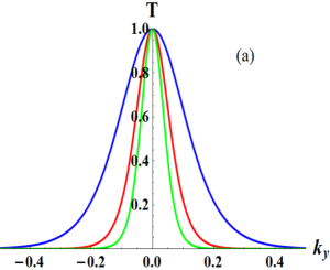
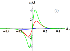
Figure 4: Transmission probability (a) and Goos-Hänchen shifts (b) as function of transverse wave vector $k_{y}$, around the Dirac point ($E=V_{B}+\tau$), for single (blue line), double (red line) barrier and graphene superlattices (green line), where physical parameters are chosen to be $\Delta_{B}=0$, $d_{W}=d_{B}=7nm$, $V_{B}=10\gamma$ and $V_{W}=4\gamma$.

4.2 Single barrier structure

We consider electron in AA-stacked BLG scattered by single barrier structure in the absence of the gap. In Figure 5, we present the density plot of the transmission probability and GH shifts as a function of the incident angle and its energy corresponding to the upper ($\tau=+1$) and lower ($\tau=-1$) cones, for $\Delta_{B}=0$, $d_{B}=7nm$ and $V_{B}=10\gamma$. Recall that for AA-stacked BLG the band structure is composed of two Dirac cones shifted by $\tau$. From Figure 5, we see that the transmission and the GH shifts, for both cones, has the same form as that in the case of monolayer graphene [23]. Obviously, the GH shifts can be positive as well as negative and are closely related to the transmission gap.

• Figure 5(b) and 5(d) indicates that, for positive incident angle, the GH shifts are negative for $E<V_{B}+\tau$, positive for $E>V_{B}+\tau$, change the sign near the Dirac point, $E=V_{B}+\tau$ and become large at some resonance points. Since the GH shifts are bilaterally asymmetrical with respect to the normal incidence, for negative incident angle, the shifts are positive for $E<V_{B}+\tau$ and negative for $E>V_{B}+\tau$.

• Figures 5(a) and 5(c) show that there is perfect transmission for normal or near normal incidence ($\phi_{0}^{\tau}\rightarrow 0$), which is a manifestation of the Klein tunneling [3]. We notice that the angular dependence of the transmission probability is very remarkable. Moreover, the transmission is bilaterally symmetrical with respect to the normal incidence.

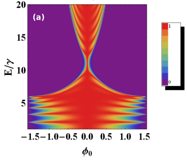
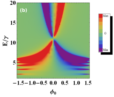
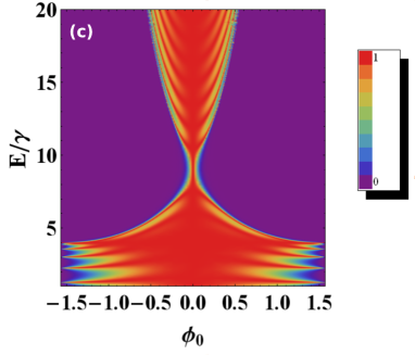
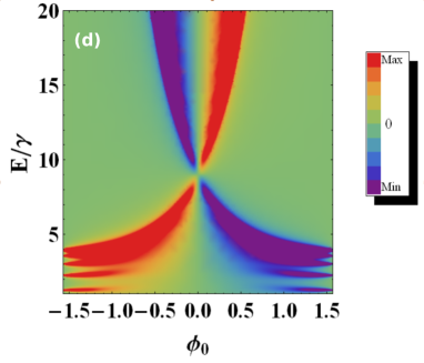
Figure 5: Density plot of the transmission probability and Goos-Hänchen shifts as function of the energy for single barrier, with physical parameters $\Delta_{B}=0$, $d_{B}=7nm$ and $V_{B}=10\gamma$. $\tau=1$ for (a, b), $\tau=-1$ for (c, d).

4.3 Double barrier structure

Now we consider a double barrier structure, the transmission probability and GH shifts as a function of the incident angle and its energy for both cones are presented in Figure 6. The physical parameters are chosen to be $\Delta_{B}=0$, $d_{W}=2d_{B}=14nm$, $V_{B}=10\gamma$ and $V_{W}=4\gamma$.

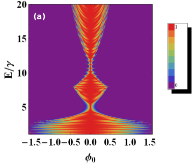
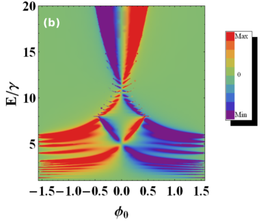
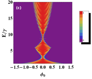
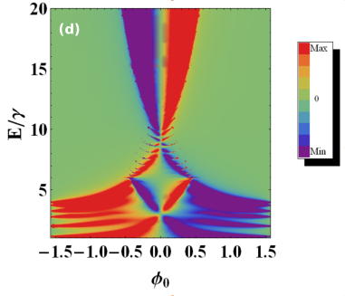
Figure 6: Density plot of the transmission probability and Goos-Hänchen shifts as function of the incident angle and its energy for double barrier structure, with physical parameters $\Delta_{B}=0$, $d_{W}=2d_{B}=14nm$, $V_{B}=10\gamma$ and $V_{W}=4\gamma$. $\tau=1$ for (a,b), $\tau=-1$ for (c,d).

Figures 6(a,c) correspond to the transmission, while 6(b,d) correspond to the GH shifts for the upper ($\tau=+1$) and lower ($\tau=-1$) cones, respectively. Compared to the results of single barrier, there is a new Dirac point, which appears at $E=V_{W}+\tau$ that is resulting from the chiral nature of massless Dirac excitations. It is clearly seen that the transmission displies sharp peaks inside the transmission gap around the Dirac point located at $E=V_{B}+\tau$, while they are absent around the new Dirac point located at $E=V_{W}+\tau$ that corresponds to the first transmission gap. We notice that, the transmission resonances are resulting from the available states in the well between the barriers. For positive incident angle, the GH shifts are negative for $E<V_{W}+\tau$ and positive for $E>V_{B}+\tau$. However, for $V_{W}+\tau<E<V_{B}+\tau$ the shifts shows different behaviors, which are positive and negative, respectively. In addition, the shifts display sharp peaks, that are equal to that of the transmission resonances, inside the transmission gap around $E={V_{B}}+\tau$. While, these peaks are absent around the second Dirac points $E={V_{W}}+\tau$. On the other hand, compared to our previous work [20], we found a strong similarities with respect to the monolayer case.

4.4 Graphene superlattices

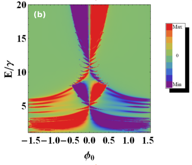
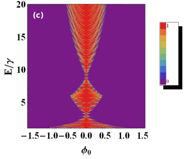
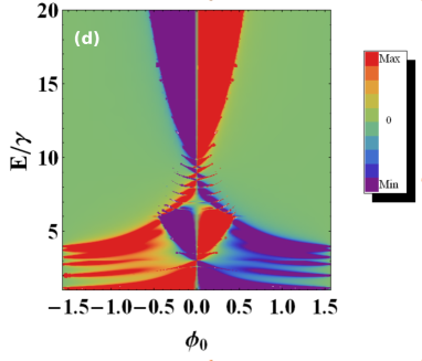
Figure 7: Density plot of the transmission probability and Goos-Hänchen shifts as function of the incident angle and its energy for graphene superlattices structure ($(BW)^{5}B(WB)^{5}$), with physical parameters $\Delta_{B}=0$, $d_{W}=2d_{B}=14nm$, $V_{B}=10\gamma$ and $V_{W}=4\gamma$. $\tau=1$ for (a,b), $\tau=-1$ for (c,d)

Let us consider a graphene SLs composed of 11 barriers and 10 wells denoted by $(BW)^{5}B(WB)^{5}$. To underline the behaviors of the transmission and GH shifts in terms of the incident angle and its energy, we plot Figure 7, with the same physical parameters as in Figure 6. Compared to the results shown for double barrier structure, we notice that there are the same positions of the Dirac points for each individual cone. For positive incident angle (when $E<V_{W}+\tau$ and $E>V_{B}+\tau$), the shifts are respectively, in the forward and backward directions, which is due to the fact that the signs of group velocity are opposite. We observe that peaks in transmission gap appear and the GH shifts display sharp peaks inside the transmission gap around the Dirac point located at $E=V_{W}+\tau$, both of results are absent in the case of double barrier structures. One can see that the number of sharp peaks of the shifts is equal to that of transmission resonances around the two Dirac points. It is interesting to note that for graphene SLs, we have more then one Dirac point located at the same position, while the position of the Dirac point is the same whatever the number of the barriers. Like single and double barrier structures, the transmission is bilaterally symmetrical with respect to the normal incidence. In addition, we notice that as observed in [20, 23], the GH shifts are related to the transmission gap around the two Dirac points.

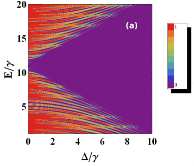
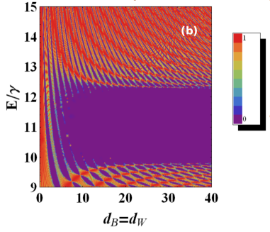
Figure 8: Density plot of transmission probability as function of the gap and the interbarrier $d_{B}=d_{W}$ and energy $E$, with $V_{W}=4\gamma$, $V_{B}=10\gamma$, $\tau=1$ and ${\phi_{0}^{+1}}=4^{\circ}$. $d_{B}=d_{W}=14nm$ for (a), $\Delta_{B}=1\gamma$ for (b).

Now, we will turn to discus the influence of the gap and the width $d_{B}=d_{W}$ on the transmission for graphene SLs. Note that, the gap is introduced, as shown in Figure 1, in the barrier regions. In Figure 8(a), we show the density plot of the transmission as function of the gap $\Delta_{B}$ and energy $E$. This has been performed by fixing the parameters $V_{W}=4\gamma$, $V_{B}=10\gamma$, $\tau=1$, $\phi^{+1}_{0}=4^{\circ}$ and $d_{B}=d_{W}=7nm$. For zero gap, one can see that the transmission exhibits sharp peaks around the two Dirac points $E=V_{B}+1$ and $E=V_{W}+1$. By increasing $\Delta_{B}$, the transmission gap around the Dirac point located at $E=V_{B}+1$ increases. We also observe that the transmission exhibits some oscillation and vanishes after that. It is worth to see how the barrier width $d_{B}=d_{W}$ will affect the transmission probability, this is shown in Figure 8(b). We choose the same physical parameters like in Figure 8(a) with gap $\Delta_{B}=1\gamma$. As we have already seen in Figure 8(a), we have a transmission gap around the Dirac point located at $E=V_{B}+1$. In addition, there exists a sharp transmission peaks and the location of such peaks is changed by the interbarrier width.

4.5 Graphene superlattices with defect

Now, we consider a gapless graphene SLs $(BW)^{5}D(WB)^{5}$ with a defect $D$. Figure 9 presents the numerical results of the transmission and GH shifts for the upper cone ($\tau=+1$) in terms of the incident angle and its energy for graphene SLs with defect. We should emphasize, that for the lower cone ($\tau=-1$) we obtain the same form as for $T^{+1}$ and $s_{t}^{+1}$ but just shifted down. In such structure, one can clearly end up with an interesting result such that, in addition to the two Dirac points found in the case of graphene SLs, it has a third Dirac point located at $E=V_{D}+\tau$. Additionally, we have more then one Dirac point located at the same position for $E=V_{B}+\tau$ and $E=V_{W}+\tau$, but we have only one Dirac point located at $E=V_{D}+\tau$. Similar to the case with defect (Figures 7(b,d)), we observe that the shifts display sharp peaks inside the transmission gap around the two Dirac points located at $E=V_{B}+\tau$ and $E=V_{W}+\tau$, which are absent in the transmission gap around $E=V_{D}+\tau$.

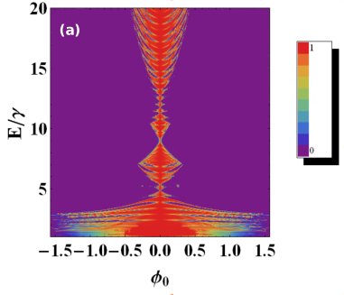
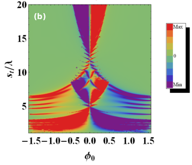
Figure 9: Density plot of the transmission probability (a) and Goos-Hänchen shifts (b) as function of the incident angle and its energy for graphene superlattices $(BW)^{5}D(WB)^{5}$ with defect $D$. $\Delta_{B}=0$, $\Delta_{D}=0$, $d_{W}=2d_{B}=14nm$, $d_{D}=30nm$, $V_{B}=11\gamma$, $V_{W}=4\gamma$ and $V_{D}=8\gamma$.

4.6 Influence of the potential height $V_{D}$

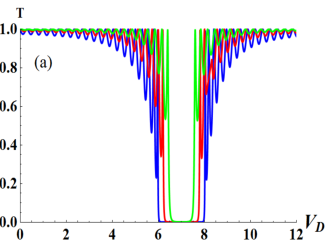
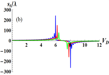
Figure 10: Transmission probability (a) and Goos-Hänchen shifts (b) as function of the potential height $V_{D}$ for graphene superlattices $(BW)^{5}D(WB)^{5}$ with defect $D$. $\Delta_{B}=0$, $d_{W}=2d_{B}=14nm$, $d_{D}=30nm$, $V_{B}=11\gamma$, $V_{W}=0$, $\tau=1$, $\phi_{0}{{}^{+1}}=4^{\circ}$ (green line), $\phi_{0}{{}^{+1}}=6^{\circ}$ (red line), $\phi_{0}{{}^{+1}}=8^{\circ}$ (blue line) and $E=8\gamma$.

Now let us see how the potential height $V_{D}$ of defect in gapless graphene SLs affects the transmission $T^{+1}$ and GH shifts $s_{t}^{+1}$. These two quantities are shown in Figure 10 for $d_{W}=2d_{B}=14nm$, $d_{D}=30nm$, $V_{B}=11\gamma$, $V_{W}=0$, $\tau=1$, $E=8\gamma$ and three different values of the incident angle $\phi^{+1}_{0}=4^{\circ},\ 6^{\circ},\ 8^{\circ}$. Figure 10(b) shows that the GH shifts change the sign at the Dirac point $E=V_{D}+1$. One can see that, there is a strong dependence of the GH shifts on the incident angle. Indeed, by increasing the incident angle the maximum absolute value of the shifts increase and the transmission gap becomes larger. We notice that the GH shifts are positive as long as the condition $E-\tau>V_{D}$ is satisfied and negative if $E-\tau<V_{D}$. For large value of $V_{D}$, the GH shifts become mostly constant. We deduce that there is a strong dependence of the GH shifts on the potential height $V_{D}$, which can help to realize controllable negative and positive GH shifts. From Figure 10(a), we clearly see that the transmission gap becomes larger by increasing the incident angle. In addition, by increasing $V_{D}$ both transmission and GH shifts exhibits an oscillatory behavior in terms of the potential $V_{D}$.

5 Conclusion

We investigated the transmission and Goos-Hänchen shifts for the Dirac fermions transmitted through AA-stacked bilayer graphene superlattices with a periodic potentials of square barriers. We started by formulating our Hamiltonian model that describes the system under consideration and getting the associated energy bands. The obtained bands are composed of two Dirac cones shifted up and down by the interlayer coupling $\gamma$.

Using the transfer matrix method, we calculated the transmission and the Goos-Hänchen shifts. These two quantities were investigated in different graphene-systems: single, double barriers and graphene superlattices. We obtained two transmissions and two shifts corresponding to the upper and lower cones. The total transmission is the average of the two transmissions and the same for the total Goos-Hänchen shifts. Moreover, we found that the two transmissions and the two Goos-Hänchen shifts, for both cones, have the same form as that in the case of monolayer graphene but shifted up and down by $\tau$.

Subsequently, it has been shown that Klein tunneling of an electron can occur at normal incidence, for single, double barriers and graphene superlattices. Also, we have found that the shifts can be positive as well as negative and change the sign at the Dirac points. Moreover, by increasing the number of barriers, the maximum absolute values of the shifts increase. In the case of double barrier structures and graphene superlattices, exist extra Dirac points located at $E=V_{W}+\tau$, as compared to the case of single barrier, where we have only one Dirac point located at $E=V_{B}+\tau$. In addition, for the case of graphene superlattices, there is more than one Dirac point at the same position. For such structure, the Goos-Hänchen shifts display sharp peaks inside the transmission gap around the two Dirac point $E=V_{B}+\tau$ and $E=V_{W}+\tau$. We ended up with an interesting result such that the number of sharp peaks is equal to that of transmission resonances. We noticed that the sharp peaks are absent around the Dirac point $E=V_{W}+\tau$ in the case of double barrier structure. These results are in agrement with those of monolayer graphene obtained in our previous work [20].

Furthermore, we showed that the shifts can be modulated by the height of potential barrier and also can be enhanced by the presence of resonant energies, which have potential applications in various graphene-based electronic devices [34, 35, 36]. In addition, we also investigated the Goos-Hänchen shifts for graphene superlattices with a defect. It is observed that the negative or positive shifts can be enhanced and controlled by the potential height of defect. The Goos-Hänchen shifts discussed her may have potential applications in the control of electron beams in the fields of various graphene based electronic devices.

References

- [1] K. S. Novoselov, A. K. Geim, S. V. Morozov, D. Jiang, Y. Zhang, S. V. Dubonos, I. V. Grigorieva and A. A. Firsov, Science 306, 666 (2004).
- [2] A. K. Geim and K. S. Novoselov, Nat. Mater. 6, 183 (2007).
- [3] M. I. Katsnelson, K. S. Novoselov and A. K. Geim, Nat. Phys. 2, 620 (2006).
- [4] C. J. Tabert and E. J. Nicol, Phys. Rev. B 86, 075439 (2012).
- [5] T. Ando and J. Phys. Conf. Ser. 302, 012015 (2011).
- [6] Y.-F. Hsu, G.-Y. Guo, Phys. Rev. B 82, 165404 (2011).
- [7] E. Prada, P. San-Jose, L. Brey and H. Fertig, Solid State Commun. 151, 1065 (2011).
- [8] A. L. Rakhmanov, A. V. Rozhkov, A. O. Sboychakov and F. Nori, Phys. Rev. Lett. 109, 206801 (2012).
- [9] L. Brey and H. A. Fertig, Phys. Rev. B 87, 115411 (2013).
- [10] Z. Liu, K. Suenaga, P. J. F. Harris and S. Iijima, Phys. Rev. Lett. 102, 015501 (2009).
- [11] J. Borysiuk, J. Sołtys and J. Piechota, J. Appl. Phys. 109, 093523 (2011).
- [12] P. L. de Andres, R. Ramírez and J. A. Vergs, Phys. Rev. B 77, 045403 (2008).
- [13] F. Goos and H. Hänchen, Ann. Phys. 436, 333 (1947).
- [14] F. Goos and H. Hänchen, Ann. Phys. 6, 251 (1949).
- [15] K. Artmann, Ann. Phusik 2, 87 (1949).
- [16] R. Briers, O. Leroy and G. Shkerdinb, J. Acoust. Soc. Am. 108, 1624 (2000).
- [17] L.-G. Wang and S.-Y. Zhu, Appl. Phys. B 98, 459 (2010).
- [18] V.-O. de Haan, J. Plomp, T. M. Rekveldt, W. H. Kraan, A. A. van Well, R. M. Dalgliesh and S. Langridge, Phys. Rev. Lett. 104, 010401 (2010).
- [19] C. W. J. Beenakker, R. A. Sepkhanov, A. R. Akhmerov and J. Tworzydło, Phys. Rev. Lett. 102, 146804 (2009).
- [20] A. Jellal, I. Redouani, Y. Zahidi and H. Bahlouli, Phys. E 58, 30 (2014).
- [21] A. Jellal, Y. Wang, Y. Zahidi and M. Mekkaoui, Phys. E 68, 53 (2015).
- [22] X. Chen, P.-L Zhao and X.-J Lu, Eur. Phys. J. B 86, 223 (2013).
- [23] X. Chen, J.-W. Tao and Y. Ban, Eur. Phys. J. B 79, 203 (2011).
- [24] A. Zubarev and D. Dragoman, Phys. E 44, 1687 (2012).
- [25] Z. P. Niu, F. X. Li, B. G. Wang, L. Sheng and D. Y. Xing, Eur. Phys. J. B 66, 245 (2008).
- [26] M. Barbier, P. Vasilopoulos and F. M. Peeters, Phys. Rev. B 80, 205415 (2009).
- [27] B. Van Duppen and F. M. Peeters, Phys. Rev. B 87, 205427 (2013).
- [28] M. Sanderson, Y. S. Ang and C. Zhang, Phys. Rev. B 88, 245404 (2013).
- [29] L.-G. Wang and S.-Y. Zhu, Phys. Rev. B 81, 205444 (2010).
- [30] D. Bohm, Quantum Theory, Prentice-Hall (New York, 1951), pp. 257-261.
- [31] A. F. Young and P. Kim, Nat. Phys. 5, 222 (2009).
- [32] N. Stander, B. Huard and D. Goldhaber-Gordon, Phys. Rev. Lett. 102, 026807 (2009).
- [33] M. Barbier, P. Vasilopoulos, and F. M. Peeters, Phys. Rev. B 82, 235408 (2010).
- [34] Z. Wu, F. Zhai, F. M. Peeters, H. Q. Xu and K. Chang, Phys. Rev. Lett. 106, 176802 (2011).
- [35] F. Zhai, Y.-L. Ma and K. Chang, New J. Phys. 13, 083029 (2011).
- [36] Y. Song, H.-C.Wu and Y. Guo, Appl. Phys. Lett. 100, 253116 (2012).