Infrastructure and methods for real-time predictions of the 2014 dengue fever season in Thailand

Abstract

Epidemics of communicable diseases place a huge burden on public health infrastructures across the world. Producing accurate and actionable forecasts of infectious disease incidence at short and long time scales will improve public health response to outbreaks. However, scientists and public health officials face many obstacles in trying to create accurate and actionable real-time forecasts of infectious disease incidence. Dengue is a mosquito-borne virus that annually infects over 400 million people worldwide. We developed a real-time forecasting model for dengue hemorrhagic fever in the 77 provinces of Thailand. We created an operational and computational infrastructure that generated multi-step predictions of dengue incidence in Thai provinces every two weeks throughout 2014. These predictions show mixed performance across provinces, out-performing naïve seasonal models in over half of provinces at a 1.5 month horizon. Additionally, to assess the degree to which delays in case reporting make long-range prediction a challenging task, we compared the performance of our real-time predictions with predictions made with fully reported data. This paper provides valuable lessons for the implementation of real-time predictions in the context of public health decision making.

1 Introduction

Producing accurate and actionable forecasts of infectious disease incidence at short and long time scales will improve public health response to outbreaks. Real-time forecasts of infectious disease outbreaks can facilitate targeted intervention and prevention strategies, such as increased healthcare staffing or vector control measures. However, we currently have a limited understanding of the best ways to integrate forecasts into real-time public health decision-making.

Dengue is a mosquito-borne infectious disease that places an immense public health and economic burden upon countries around the world, especially in tropical areas. A severe form of the disease, dengue hemorrhagic fever (DHF), may lead to debilitating pain, organ shock, and even death [1]. Currently over 2.5 billion individuals worldwide are at risk of infection with dengue, a mosquito-borne RNA virus [2]. Global incidence of dengue has increased significantly over the past few decades, with estimated annual global incidence of about 400 million infections each year [3].

Dengue is endemic in Thailand, which has 77 provinces including one large municipality (Bangkok). National annual incidence rates of reported dengue in Thailand range between 30 cases per 100,000 population and 224 cases per 100,000 population [4]. Some estimates suggest that between 50-80% of cases may be inapparent and hence are difficult to detect clinically and often go unreported [5, 6, 7]. Annual outbreaks show dynamic temporal and spatial patterns, with great year-to-year and across-province variation, making public health planning and resource allocation an ongoing challenge [8, 9].

With the maturation of disease surveillance and reporting systems in recent years, real-time disease forecasting has become a realistic goal in some settings. Recognizing the importance of this emerging field, several governmental agencies have established disease prediction contests in recent years, with the goal of having contestants produce accurate forecasts: e.g. a 2013 CDC influenza prediction challenge [10], a 2014 DARPA chikungunya prediction challenge [11], and a 2015 NOAA and White House dengue prediction challenge [12]. However, researchers and practitioners are still working to understand and establish a set of best practices for implementing real-time prediction algorithms in practice.

Creating predictions in real-time poses operational, computational, and statistical challenges. Operationally, raw data must be made available in a standard format for processing into analysis datasets. Historical data is also needed to allow for training of the prediction model(s). To enable transparent evaluations, predictions should be formally registered and archived in a publicly available database. Computational infrastructure is needed to transform and/or merge raw data into the analysis dataset and to run the models themselves. Analytical challenges include appropriate model training, selection, and validation, considering adjustments for delayed or incomplete case reporting. Depending on the methods used, additional statistical work may be necessary to accurately report uncertainty in the reported predictions. Below, we describe our approaches to dealing with these challenges.

In this manuscript we present the results from the first year of forecasting DHF across the 77 provinces in Thailand. In 2014 our research team, a collaboration of the Ministry of Public Health of Thailand and researchers from multiple academic institutions, implemented a system for generating real-time forecasts of DHF based on current disease surveillance reports from Thailand. This paper illustrates several key components of a successful real time prediction framework, including:

• a reliable pipeline for data transfer, cleaning, and analysis, with a data storage architecture that can recreate datasets that were available at a particular time (Section 2),

• a statistical model of disease transmission used to generate real-time predictions of infectious disease incidence (Section 3),

• an appropriate and rigorous model validation framework, including aggregating evaluations across location, calendar time, and prediction horizon (Section 4), and

• an assessment of the impact of case reporting delays on the accuracy of predictions (Sections 3.3 and 4.2).

Valuable efforts have been made to create, validate, and operationalize real-time influenza predictions for the US [13], although these efforts have not faced the same challenges of systematic under-reported data. The operational infrastructure that we present in this manuscript provides valuable lessons for other collaborative prediction efforts between public health agencies and academic partners.

2 A real-time prediction pipeline: turning data into forecasts

2.1 Data overview

The data presented here come from the national surveillance system run by the Ministry of Public Health in Thailand. Monthly dengue hemorrhagic fever (DHF) case counts for each province are available from January 1968 through December 2005. Individual case reports (hereafter referred to as “line-list” data) were available for dengue fever (DF), DHF, and dengue shock syndrome from January 1, 1999 through December 31, 2014. The line-list data contains information on each case, including date of symptom onset, home address-code of the case (similar to a U.S. zip code), disease diagnosis code, and demographic information (sex, marital status, age, etc.). In years where we had overlapping sources for case data, the line-list data were used. A summary of province-level characteristics for all provinces in Thailand is provided in the appendix. Since 1968, several provinces have split into multiple provinces. Details on how we accommodate these province separations are available in the appendix. In one instance, the counts associated with a province (Bueng Kan) that split from another (Nong Khai) in 2011 have continued to be counted with the original province since we do not yet have enough data to predict for the new province.

Theoretical work demonstrates that by choosing the generation time as the discrete time interval for case reporting, the case reports may more easily be used to model the reproductive rate of the disease [14]. The generation time for dengue is two weeks, hence we aggregated the line-list data into biweekly intervals and interpolated the monthly counts into biweekly counts. (We used a definition of biweeks that followed a standardized definition based on calendar dates. See Supplemental Table 1.) Interpolation was performed by fitting a monotonically increasing smooth spline to the cumulative case counts in each province, and then taking the differences between the estimated cumulative counts at each interval as the number of incident cases in a given interval.

We chose to use only DHF cases because: (1) DHF is the only disease reported consistently across the 47 years of data collection, (2) DHF is less likely than DF to be misdiagnosed or to be differentially detected over time, and (3) from a public health perspective, DHF is a more relevant outcome, as it is a life-threatening condition and requires medical attention.

The research aspects of this study were approved by the Johns Hopkins Bloomberg School of Public Health and University of Massachusetts Amherst institutional review boards.

2.2 Real-time data management

We established a secure data transfer process to transmit data from the Thai disease surveillance system to U.S. researchers. Throughout the 2014 calendar year, Thai public health officials transmitted data approximately every two weeks to a secure server based in Baltimore, Maryland (Supplemental Table 2). These data were then loaded into a PostgreSQL database containing all of the data, including monthly case counts and a table with all line-list data received to date. The final report containing a cleaned and finalized record of all cases for the 2014 season was delivered in April 2015. As of that time, this database held records of 2,586,928 unique cases of dengue in Thailand for the years 1968 through 2014, including records of 1,930,858 DHF cases (Figure 1).

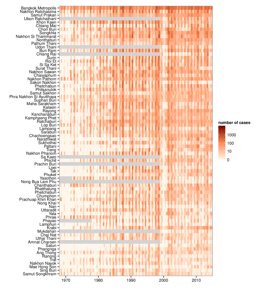
Figure 1: Raw dengue hemorrhagic fever case counts for 77 provinces of Thailand across 47 years (1968 - 2014). Provinces are ordered by by population (larger populations on the top). Gray regions indicate periods of time when a province was not in existence.

When forecasting, we will only ever have the cases recorded prior to the time the predictions are made. So that we could compare the expected real-time performance of models as if they had been applied in real-time, all data were archived in the database with a time-stamp on arrival. This enabled researchers to “turn back the clock”, i.e. to query data that was available at a particular point in time. Throughout this manuscript, we use the term “nowcast” to refer to predictions made for timepoints on or prior to the analysis date and “forecasts” to refer to predictions made for timepoints at or after the analysis date.

2.3 Accounting for delays in case reporting

A key property of a surveillance system is the reporting delay, defined for our purposes as the duration of time between symptom onset and the case being available for analysis. During 2014 reporting delays for dengue ranged from 1 to 50 weeks. This was due to the process of reporting cases. Case reports typically follow a path of reporting from hospitals to district surveillance centers and then to provincial health offices before arriving at the national surveillance center. In all provinces, 50% of cases were reported within 6 weeks and 75% of cases were reported within 10 weeks. However, a small fraction of cases took quite a bit longer. To account for reporting delays, our models specified a reporting lag $l$, in biweeks. Data with onset dates within last $l$ biweeks was considered underreported and left out from the analysis. We present results from the models with a lag of 6 biweeks (about 3 months), as these produced stable predictions across the entire country. More sophisticated adjustments for reporting delays are the subject of our team’s ongoing research.

2.4 Timing of predictions

While the predictions presented in this manuscript were made retrospectively, in 2015 when complete data were available, they were constructed to mimic real-time predictions by using only the data available at each analysis date in 2014. During the 2014 calendar year, predictions from a similar model were generated in real-time and disseminated to the Thai Ministry of Public Health. We chose the set of analysis dates as the first day of each biweek for which data had been delivered in the previous biweek (Supplementary Table 2). For each analysis date in 2014, we used the candidate model to generate “real-time” province-level biweekly predictions for the subsequent 10 biweeks (5 months).

3 Methodology for predicting case counts

3.1 Disease model: features and estimation

Statistical model

We assumed the biweekly province-level reported cases follow a Poisson distribution, where the previous biweek’s reported cases serve as an offset term. Let the number of cases with onset occurring within time interval $t$ in province $i$ be represented as a random variable $Y_{t,i}$, then

$$Y_{t,i} \sim Poisson(\lambda_{t,i}\cdot y_{t-1,i})$$

where the lag-1 term $y_{t-1,i}$ is used as an offset in this model. We adopt the convention of using lower-case $y_{t,i}$ to indicate previously observed case counts that are treated as fixed inputs in our model. We explicitly model the rate $\lambda$ as

$$\log\lambda_{t,i} = f(b(t))+g(t)+\sum_{j\in\mathcal{C}}\sum_{k\in\mathcal{L}}\alpha_{j,k}\log\frac{y_{t-k,j}+1}{y_{t-k-1,j}+1}$$ (1)

where $\mathcal{C}$ is the set of $J$ most-correlated provinces with province $i$ and $\mathcal{L}$ is the set of lag times used in the model; $b(t)$ is the biweek of time $t$; $f(b(t))$ is assumed to be a cyclical cubic spline with period of one year (i.e. 26 biweeks); and $g(t)$ is a smooth spline to capture secular trends over time. Adding 1 to the numerator and denominator of the correlated province covariates ensures that the quantities are defined when no case counts are observed at a particular province-biweek. This method of adjusting for zero counts has been interpreted as an “immigration rate” added to each observation [15].

We note that the model can be expressed as

$$\lambda_{t,i}=\mathbb{E}\left[\frac{Y_{t,i}}{y_{t-1,i}}|y_{t-1,i}\right]\approx R_{t,i}$$ (2)

which shows that $\lambda_{t,i}$ can be interpreted as the expected reproductive rate at time $t$ in location $i$, or $R_{t,i}$ [14].

These models were fit using the Generalized Additive Model (GAM) framework (i.e. as generalized linear models with smooth splines estimated by penalized maximum likelihood) [16], using the mgcv package for R [17, 18]. Each province’s time-series was subset to remove any cases from the previous $l$ biweeks. The remaining data were smoothed before fitting the model and making predictions.

Seasonal patterns were modeled using a penalized cubic regression spline, constrained to have a cycle of one year with continuous second derivatives at the endpoints. Secular trends were modeled using penalized cubic splines with 5 equally spaced knots over 47 years (roughly one knot per decade).

Information on epidemic progression elsewhere in the country was taken into account by including reported case counts at 1 lagged timepoint for the 3 most correlated provinces with province $i$ in the data used to fit the model. Details of this model selection are provided in the appendix.

We approximated the predictive distribution for all provinces using sequential stochastic simulations of the joint distribution of the case counts for each province. Prediction intervals were generated by taking quantiles (e.g., the 2.5% and 97.5%) of this distribution. Full details of the methods used to generate the multi-step predictions are available in the appendix.

3.2 Metrics for evaluating predictions

We used several different metrics for evaluating our predicted case counts. We calculated Spearman correlation coefficients to measure the agreement between predicted and observed values. We also calculated the mean absolute error (MAE) by aggregating across analysis times within a given province. We computed the relative mean absolute error (relative MAE) comparing the predictions for a given province to predictions from a seasonal average baseline model. The seasonal baseline model for a given province is the median value of previously observed counts for the given biweek in that province over the past 10 years. The use of absolute error metrics over squared error metrics has been encouraged to enhance interpretability [19, 20]. Additionally, we calculated empirical 95% prediction interval coverage as the fraction of times the 95% prediction interval covered the true value.

3.3 Real-time vs. full-data predictions

We evaluated the performance of our real-time forecasts against predictions that could have been made had a full dataset been available at the analysis dates. To make this comparison, we ran a set of multi-step forecasts for 2014 at each analysis date using the complete data for 2014 that was finalized in late April 2015. This experiment was designed to focus on two comparisons. First, we aimed to compare real-time and full-data predictions where the multi-step predictions began at the same timepoint. Second, we aimed to compare, by horizon, the real-time and full-data predictions where the origin of the multi-step full-data predictions was anchored at the analysis time but the origin of the real-time predictions was 6 biweeks earlier to account for underreported data.

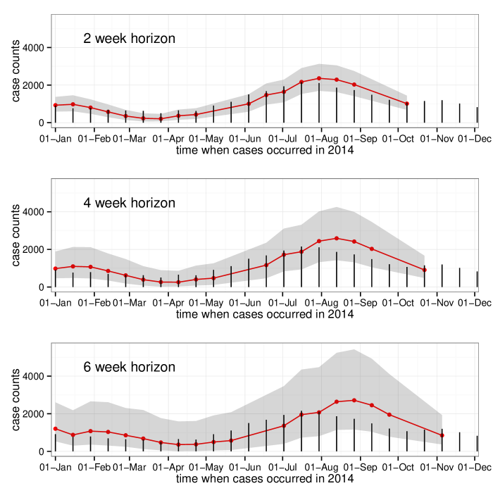
Figure 2: Country-wide real-time predictions for incident dengue hemorrhagic fever. Red lines show predicted case counts, black bars show cases reported by the end of the 2014 reporting period. The three figures show (top to bottom) one-, two-, and three-biweek ahead predictions. So, for example, every dot on the top graph is a one-biweek ahead real-time prediction made from all available data at the time of analysis.

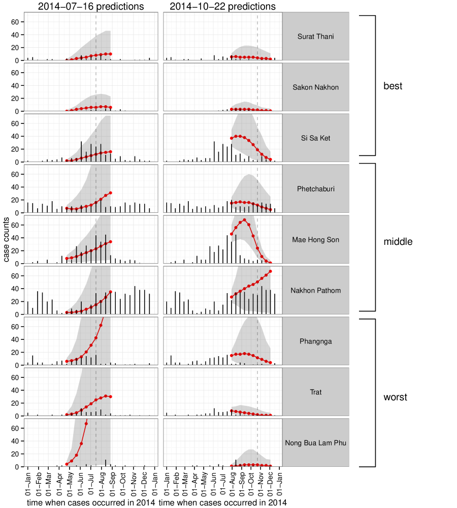
Figure 3: Ten-step forward predictions made at two time-points in 2014. Results for nine provinces are shown, representing (from top to bottom) the best three provinces, the middle three, and the worst three performing provinces in terms of relative mean absolute error when compared to a seasonal reference model.

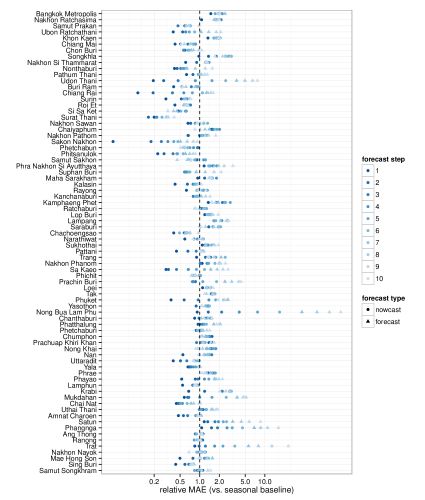
Figure 4: Relative mean absolute error (MAE) comparing our prediction model vs. a model that predicts a seasonal average, by province and step forward (in biweeks).

			relative MAE (real-time vs. seasonal baseline)
horizon (h)	$R^{2}$	95% PI coverage	$Q_{5}$	$Q_{25}$	$Q_{50}$ (median)	$Q_{75}$	$Q_{95}$
1	0.92	0.61	0.22	0.46	0.70	1.07	1.49
2	0.90	0.93	0.28	0.60	0.90	1.25	1.79
3	0.89	0.99	0.43	0.68	0.96	1.48	2.18
4	0.84	0.99	0.56	0.83	1.09	1.42	2.45
5	0.79	0.99	0.53	0.83	1.16	1.55	2.81
6	0.73	1.00	0.55	0.87	1.22	1.70	3.02
7	0.65	0.99	0.58	0.88	1.22	1.67	3.70
8	0.57	0.99	0.61	0.94	1.16	1.72	4.73
9	0.52	0.99	0.57	0.95	1.21	1.83	5.93
10	0.50	0.99	0.54	0.91	1.27	1.92	7.91

Table 1: Summary of real-time prediction accuracy, by prediction horizon. These results are aggregated across all provinces. The $R^{2}$ and 95% PI coverage columns present the overall correlation coefficient and prediction interval coverage. The relative MAE columns show five quantiles of the distribution of province-level relative MAEs comparing the real-time model at the given horizon to a seasonal baseline model at the given horizon: $Q_{5}$ (the 5^th percentile), $Q_{25}$ ($25^{th}$ percentile), $Q_{50}$ (median), $Q_{75}$ ($75^{th}$ percentile), and $Q_{95}$ (the 95th percentile). The relative MAEs were calculated as the MAE from the real-time predictions divided by the MAE from the seasonal average predictions, therefore values larger than 1 indicate that the real-time models showed more absolute error on average than the seasonal models.

4 Forecast results from 2014

4.1 Summary of province-level forecasts

In general, the model predictions showed good, if overconfident, performance at short horizons but less accuracy and high uncertainty at longer horizons. Across all provinces, the correlation between observed and predicted values was 0.92 at a horizon of 1 biweek (2 weeks) and 0.5 at a horizon of 10 biweeks, or approximately 5 months (see Table 1). Across all provinces, observed 95% prediction interval coverage was lower than expected at horizons of 2 and 4 weeks (61% and 93%, respectively), showing that the models were overconfident in their short-term predictions. This prediction interval coverage increased to 99% at a 6 week (3 biweek) prediction horizon, and remained at that level for longer horizons. This indicates that our models often had an abundance of uncertainty at mid- and long-term horizons. Figure 2 shows case counts and predictions aggregated across all provinces at horizons of 2, 4, and 6 weeks (or 1, 2, and 3 biweeks).

Figure 3 shows examples of multi-step predictions from two analysis dates in 2014. We show the results from nine distinct provinces, representing the best three provinces, the middle three provinces, and the worst three provinces in terms of relative MAE when compared to a seasonal reference model. The increasing uncertainty is visible in many cases, even when the point-predictions remain close to the true values. The explosive forecasts tended to occur more frequently in the early- and mid-season, when the historical seasonal trend rises and when the observed case counts tend to be increasing from one biweek to the next.

There was substantial variation in predictive performance across provinces. Figure 4 shows the relative mean absolute error (relative MAE) of model predictions compared to a seasonal baseline model at prediction horizons of 2 through 20 weeks (1 through 10 biweeks). We note that predictions during the first three months are nowcasts, as the most recent 6 biweeks of data are ignored in the fitting process and predictions are made starting from the point at which full data was assumed.

To compare predictive performance of our model between provinces, we used the relative MAE with a simple seasonal model as a baseline. Table 1 summarizes relative MAEs by prediction horizon. Relative to seasonal baseline prediction models, a majority of provinces made better predictions on average than the seasonal model at a 2, 4, and 6 weeks (i.e. 1, 2, and 3 biweeks) prediction horizons (i.e. up to 1.5 months from the starting point of the predictions). Up to about 5 months from the origin of the multi-step predictions (and two months from the analysis time), over 25% of province-specific models made predictions that were on average better than the seasonal baseline model. Some province-specific models showed substantially worse predictions when compared to a seasonal baseline at these longer prediction horizons (Table 2). No single province feature (e.g. total average cases, strength of seasonal trends, population size, season-to-season variation) was able to explain the substantial variations in performance, highlighting the challenges of creating a unified modeling framework for a set of varied locations (see appendix for details).

	relative MAE (real-time vs. full-data baseline)
horizon	$Q_{5}$	$Q_{25}$	$Q_{50}$ (median)	$Q_{75}$	$Q_{95}$
1	0.82	0.92	0.98	1.03	1.13
2	0.79	0.91	0.98	1.01	1.16
3	0.77	0.91	0.96	1.01	1.17
4	0.77	0.91	0.97	1.01	1.10
5	0.83	0.90	0.97	1.00	1.10
6	0.82	0.93	0.99	1.03	1.11
7	0.82	0.94	1.00	1.06	1.16
8	0.82	0.95	1.03	1.09	1.20
9	0.84	0.93	1.03	1.13	1.28
10	0.85	0.96	1.05	1.18	1.36

Table 2: Comparison of province-level prediction accuracy between full-data and real-time predictions, by prediction horizon. These calculations assume that both the full-data and real-time multi-step predictions began at the same time. The table shows the 5th percentile ($Q_{5}$), 25th percentile ($Q_{25}$), median ($Q_{50}$), 75th percentile ($Q_{75}$), and 95th percentile ($Q_{95}$) value of the relative MAE from each province at the given horizon. The relative MAEs were calculated as the MAE from the real-time predictions divided by the MAE from the full-data predictions, i.e. values larger than 1 indicate that the real-time models showed more absolute error on average than the full-data models.

	relative MAE (real-time vs. full-data baseline)
absolute horizon	$Q_{5}$	$Q_{25}$	$Q_{50}$ (median)	$Q_{75}$	$Q_{95}$
1	0.92	1.21	1.49	2.05	6.62
2	0.76	0.98	1.27	1.79	6.40
3	0.66	0.91	1.19	1.88	5.45
4	0.55	0.90	1.32	1.87	4.96

Table 3: Comparison of province-level prediction accuracy between full-data and real-time predictions, by prediction horizon. These results were computed comparing predictions as if the full data was available at the analysis time with the real-time predictions that build in a 6-biweek (approximately 3 month) buffer to account for delayed case data. The table shows the 5th percentile ($Q_{5}$), 25th percentile ($Q_{25}$), median ($Q_{50}$), 75th percentile ($Q_{75}$), and 95th percentile ($Q_{95}$) value of the relative MAE from each province at the given horizon. The relative MAEs were calculated as the MAE from the real-time predictions divided by the MAE from the full-data predictions, i.e. values larger than 1 indicate that the real-time models showed more absolute error on average than the full-data models.

4.2 Comparing real-time to full-data predictions

We compared real-time and full-data predictions that began at the same timepoint. This analysis can help answer the question of how much the real-time predictions were impacted by the underreported data, once accounting for the reporting delays by removing the most recent 3 months of data. As shown in Table 2, these analyses demonstrated that once went back 3 months to begin the nowcasting, more than 50% of the provinces had more accurate real-time forecasts than full-data forecasts at all prediction horizons up to 3 months in advance. This suggests that inaccuracies in the real-time predictions once those recent 3 months are discarded are driven less by the reporting delays than they are by model misspecification and other background noise in the data.

A second analysis compared real-time predictions with a horizon of 7 biweeks with full-data predictions at 1 biweek. This analysis can tell us how much better or worse our model would have done if we did not need to adjust for underreported data by dropping the past 3 months, i.e. if all of our data were available at the time of analysis. We refer to this realignment of horizons as the absolute horizon, to suggest that a real-time prediction that removes 6 biweeks of data and then projects 7 steps forward is predicting the same timestep as a full-data prediction that does not remove any data and just projects 1 biweek forward. Results from this analysis are shown in Table 3 for absolute horizons of 1 through 4 biweeks. Overall, 66 of the 76 provinces (87%) showed better average performance in the full-data forecasts at 1 step ahead than the real-time forecasts at 7 steps ahead (i.e. had a relative MAE of greater than 1). In a majority of the provinces at each absolute horizon the full-data forecasts were on average closer to the true value than the real-time forecasts. However across all the absolute horizons, for between 10 and 26 provinces the full-data predictions had more error than the real-time predictions. While it is surprising that full-data predictions under performed real-time predictions in such a high percentage of the provinces, this reflects the challenges of making predictions in such a noisy system. A sample of predictions by province and analysis date are provided as supplemental figures to illustrate this challenge.

5 Discussion

We present the prediction results from our real-time prediction infrastructure established for dengue hemorrhagic fever in Thailand. This infrastructure addresses several key operational features of real-time predictions, including real-time data management, the impact of reporting delays, and incorporating a disease transmission model that takes into account spatial and temporal trends.

The infectious disease prediction literature has a rich and varied selection of prediction algorithms but has not historically focused on the challenges of operationalizing predictions in real-time. Continued development and refinement of such prediction pipelines, such as that presented here, will enable existing prediction methods to reach their full potential in making an impact on public health decision-making and planning.

The infrastructure that we have developed for integrating real-time data into predictions for the Thai Ministry of Public Health is the result of a long-standing governmental/academic partnership between the Ministry and U.S.-based researchers. This collaboration has enabled the creation of a single, unified authoritative source of almost all governmental dengue surveillance ever collected in Thailand, dating back nearly 50 years [4]. Additionally, by enabling the transmitting of surveillance data in near real-time (every two weeks from October 2013 and continuing through the writing of this manuscript 2015), this effort has created a valuable dataset that has catalogued the reporting delays in a live surveillance system.

Formal data archiving protocols should be followed when making real-time predictions. Real-time predictions should be (1) generated prior to having the final data available and (2) formally registered or time-stamped in an independent data repository. Taking these steps ensures that no bias (intentional or not) enters the scientific process of evaluating the predictions.

While we are actively developing and validating other prediction models for this data, we chose to report the results from the prediction model that we used during 2014 to provide draft predictions to Thai public health officials. We intentionally did not perform extensive post hoc model validation or evaluation to minimize the risk of overfitting our model to this particular dataset.

Our 2014 real-time predictions varied substantially by province in quality and public health utility. In close to half of the Thai provices, our model out-performed a seasonal baseline model predicting one month in advance. As the horizon moves forward, the seasonal baseline model makes better predictions in more provinces: at a 5 month horizon, just over 25% of provinces are predicted better by our model than the seasonal model.

Our ability to make effective predictions into the future in a majority of provinces is made difficult by delayed case reporting. Our analyses show that if there were no reporting delays, our model would make substantially more accurate predictions in over 50% of the Thai provinces (Table 3).

While we have conducted extensive evaluation of the performance of our real-time predictions in 2014, this may not represent the performance of the model in other years. There is substantial year-to-year variation in annual province-level incidence in Thailand. The annual total number of cases observed in 2014 were in the lower half of previously observed annual incidence in 49 of 76 provinces. A complete characterization of our real-time model’s predictive performance will require evaluation across multiple years of data that is arriving in real-time, or with historical complete data with synthetically created reporting delays.

The simplicity of the statistical prediction models that we present in this manuscript are both a strength and a weakness. This type of phenomenological time-series model tends to show good predictive performance in the short term but have known deficiencies when making long-term predictions. Additionally, when forecasting forward from auto-regressive models, this can lead to instabilities and explosive forecasts, as was observed in the predictions from some of the provinces. Also contributing to the instability of our models in a prediction context are that we do not incorporate uncertainty in and use a smoothed value of the $y_{i,t-1}$ offset term.

The model that we present here has been shown to perform well in contexts where there are no reporting delays [manuscript in preparation]. The auto-regressive model used in this work is based on a standard statistical auto-regressive integrated moving average (ARIMA) models. In fact, the reformulation of the ARIMA model in a disease transmission model context – making explicit the connection between modeling auto-regressive counts and the reproductive number, as shown in equation 2 – is an important link between commonly used models in different fields.

The past decade of biomedical research has borne witness to rapid growth in digital surveillance data. A pressing challenge for the professional and academic epidemiological and biostatistical communities is to learn how to turn this deluge of data into evidence that informs decision making about improving health and preventing illness at the individual and population levels. Improved real-time forecasts of infectious disease outbreaks can inform targeted intervention and prevention strategies. Continued research and collaboration in this area will lead to a better understanding of how to integrate infectious disease predictions into public health practice. The collaborative effort described by this manuscript provides a template for operationalizing real-time predictions and describes specific results from this effort to integrate modern tools of data science with public health decision making.

References

- [1] D J Gubler. Dengue and dengue hemorrhagic fever. Clinical microbiology reviews, 11(3):480–496, July 1998.
- [2] World Health Organization. Dengue and severe dengue.
- [3] Samir Bhatt, Peter W Gething, Oliver J Brady, Jane P Messina, Andrew W Farlow, Catherine L Moyes, John M Drake, John S Brownstein, Anne G Hoen, Osman Sankoh, Monica F Myers, Dylan B George, Thomas Jaenisch, G R William Wint, Cameron P Simmons, Thomas W Scott, Jeremy J Farrar, and Simon I Hay. The global distribution and burden of dengue. Nature, 496(7446):504–507, April 2013.
- [4] Kriengsak Limkittikul, Jeremy Brett, and Maïna L’Azou. Epidemiological trends of dengue disease in Thailand (2000-2011): a systematic literature review. PLOS Neglected Tropical Diseases, 8(11):e3241, November 2014.
- [5] Timothy P Endy, Kathryn B Anderson, Ananda Nisalak, In-Kyu Yoon, Sharone Green, Alan L Rothman, Stephen J Thomas, Richard G Jarman, Daniel H Libraty, and Robert V Gibbons. Determinants of inapparent and symptomatic dengue infection in a prospective study of primary school children in Kamphaeng Phet, Thailand. PLOS Neglected Tropical Diseases, 5(3):e975, 2011.
- [6] Timothy P Endy, Supamit Chunsuttiwat, Ananda Nisalak, Daniel H Libraty, Sharone Green, Alan L Rothman, David W Vaughn, and Francis A Ennis. Epidemiology of inapparent and symptomatic acute dengue virus infection: a prospective study of primary school children in Kamphaeng Phet, Thailand. American journal of epidemiology, 156(1):40–51, July 2002.
- [7] Timothy P Endy, In-Kyu Yoon, and Mammen P Mammen. Prospective cohort studies of dengue viral transmission and severity of disease. Current topics in microbiology and immunology, 338:1–13, 2010.
- [8] Bernard Cazelles, Mario Chavez, Anthony J McMichael, and Simon Hales. Nonstationary influence of El Niño on the synchronous dengue epidemics in Thailand. PLOS Medicine, 2(4):e106, April 2005.
- [9] Derek A T Cummings, Rafael A Irizarry, Norden E Huang, Timothy P Endy, Ananda Nisalak, Kumnuan Ungchusak, and Donald S Burke. Travelling waves in the occurrence of dengue haemorrhagic fever in Thailand. Nature, 427(6972):344–347, January 2004.
- [10] Centers for Disease Control and Prevention. Announcement of Requirements and Registration for the Predict the Influenza Season Challenge, November 2013.
- [11] Defense Advanced Research Projects Agency. DARPA Forecasting Chikungunya Challenge, August 2014.
- [12] Pandemic Prediction and Forecasting Science and Technology Interagency Working Group. Dengue Forecating.
- [13] Jeffrey Shaman, Alicia Karspeck, Wan Yang, James Tamerius, and Marc Lipsitch. Real-time influenza forecasts during the 2012–2013 season. Nature Communications, 4, December 2013.
- [14] Hiroshi Nishiura, Gerardo Chowell, Hans Heesterbeek, and Jacco Wallinga. The ideal reporting interval for an epidemic to objectively interpret the epidemiological time course. Journal of The Royal Society Interface, 7(43):297–307, February 2010.
- [15] S L Zeger and B Qaqish. Markov regression models for time series: a quasi-likelihood approach. Biometrics, 44(4):1019–1031, December 1988.
- [16] T J Hastie and R J Tibshirani. Generalized Additive Models. CRC Press, June 1990.
- [17] S N Wood. Fast stable restricted maximum likelihood and marginal likelihood estimation of semiparametric generalized linear models. Journal of the Royal Statistical Society Series B-Statistical Methodology, 73(1):3–36, 2011.
- [18] R. Ihaka and R. Gentleman. R: A language for data analysis and graphics. Journal of computational and graphical statistics, 5(3):299–314, 1996.
- [19] Rob J Hyndman and Anne B Koehler. Another look at measures of forecast accuracy. International Journal of Forecasting, 22(4):679–688, October 2006.
- [20] N.G. Reich, Justin Lessler, Krzysztof Sakrejda, Stephen A Lauer, Sopon Iamsirithaworn, and Derek A T Cummings. Case studies in evaluating time series prediction models using the relative mean absolute error. SelectedWorks, September 2015.