Convex programming with fast proximal and linear operators

Abstract

We present Epsilon, a system for general convex programming using fast linear and proximal operators. As with existing convex programming frameworks, users specify convex optimization problems using a natural grammar for mathematical expressions, composing functions in a way that is guaranteed to be convex by the rules of disciplined convex programming. Given such an input, the Epsilon compiler transforms the optimization problem into a mathematically equivalent form consisting only of functions with efficient proximal operators—an intermediate representation we refer to as prox-affine form. By reducing problems to this form, Epsilon enables solving general convex problems using a large library of fast proximal and linear operators; numerical examples on many popular problems from statistics and machine learning show that this often improves running times by an order of magnitude or more vs. existing approaches based on conic solvers.

1 Introduction

In the field of convex optimization there has existed a fundamental dichotomy between “general purpose” and “specialized” solvers. Many robust solvers exist that can solve very general, broad classes of optimization problems (e.g. semidefinite programs, which can express a very wide range of optimization tasks), and there are modeling frameworks (e.g. CVX [11], YALMIP [13]) that can quickly express complex optimization problems by reduction to one of these forms. However, these methods typically only scale to relatively small-sized problems and largely due to these scaling problems, there has also been a great deal of work on special-purpose solvers for very particular optimization problems of interest (e.g. a particular loss function plus regularization, a particular form of sparse constraints, etc). But these approaches are very much intended for a particular form of problem, and usually require significant human effort to adapt to even slightly different formulations.

In this paper, we present Epsilon, a software architecture and system that makes a significant step toward bridging this gap. Like the above-mentioned modeling frameworks, Epsilon takes as input a convex problem specified in terms of disciplined convex programming (DCP), a specification of convex problems that can easily and intuitively express complex objectives and constraints. However, unlike current DCP systems which transform the problem into a standard conic form and then pass to a cone solver, Epsilon transforms the problem into a form we call prox-affine: a sum of “prox-friendly” functions (i.e., functions that have efficient proximal operators) composed with affine transformations. These functions include the cone projections sufficient to solve existing cone problems, but prox-affine form is a much richer representation also including a wide range of other convex functions with efficient proximal operators.

The main advantage of the prox-affine form is that it maintains significant structure from the original problem that is lost in traditional cone transformations—the Epsilon solver exploits this structure by directly implementing a large library of proximal operators and applying operator splitting techniques. In particular, we develop an approach for solving problems in prox-affine form based on the alternating direction of multipliers (ADMM) [2], but several alternative approaches are possible as well. Typically, the computational time for this algorithm (as with most iterative numerical algorithms) is dominated by the evaluation of linear operators and here we integrate a large library of linear operators which can often be far more efficient than sparse or dense matrices. In total, the resulting Epsilon system can solve a wide range of optimization problems an order of magnitude (or more) that existing approaches to general convex programming—we provide several examples of popular problems from statistics and machine learning in Section 5.

The main contributions of this paper are:

1. We develop the prox-affine form for general convex programs and provide an algorithm for converting general disciplined convex programs into prox-affine form. Using the terminology of programming language compilers, the prox-affine form can be thought of as an intermediate representation (IR) for the convex problem, and multiple transformations, which make the resulting form easier to solve, can be applied analogous to the multiple passes of an optimizing compiler.

2. We present an efficient algorithm for solving the resulting transformed problem, based upon ADMM, which solves the problem using a large library of linear and proximal operators.

3. We present efficient proximal algorithms for handling a number of non-linear operators arising from the prox-affine form. Several of these operators were also presented in the literature, but we include some additional cases as well.

4. We develop an efficient system for handling the resulting linear operators, which allows us to express complex operators such as Kronecker products (that frequently arise in these settings) without resorting to explicit instantiation of sparse/dense matrices.

5. We release an open source version of the Epsilon system, including benchmarks for many common optimization problems arising in the machine learning and statistics literature. In all cases, we show that Epsilon is substantially faster than existing approaches.

2 Background

Our work builds heavily upon two main lines of work: 1) disciplined convex programming (DCP) [10] and systems built upon these methods; 2) operating splitting techniques, specifically the alternating direction method of multipliers (ADMM) [2]. In this section we briefly review historical and recent work in these areas, highlighting how it relates to Epsilon.

2.1 Disciplined convex programming

Disciplined convex programming frameworks such as CVX [11], CVXPY [6] and Convex.jl [24] allow convex programs to be specified using a natural programming syntax. For example, the lasso problem ($\ell_{1}$-regularized least squares)

$$\operatorname*{minimize}_{x}\|Ax-b\|_{2}^{2}+\lambda\|x\|_{1}$$ (1)

with optimization variables $x$, problem data $A$, $b$, and regularization parameter $\lambda$, can be expressed simply as (here using CVXPY, which our system uses directly):

x = Variable(n)
prob = Problem(Minimize(sum_squares(A*x - b) + lam*norm1(x))

These libraries and other similar modeling frameworks (e.g. the YALMIP library [13]) have substantially lowered the barrier to quickly prototyping complex convex programs without the need to manually convert them to a form that can be fed directly into a numerical solver (e.g. a standard cone form).

The innovation of DCP methods in particular was a separation between the verification that a program is convex according to DCP ruleset, and the actual transformation to conic form (and also, naturally, a separation between these elements and the actual numerical solution). In particular, DCP methods represent expressions in the optimization problem (the objective term and all constraint terms) as abstract syntax trees (ASTs). Then, a set of composition rules can be applied to determine whether the problem is in fact a convex one. For example, suppose $f=h(g_{1}(x),\ldots,g(k(x))$, for $h:\mathbb{R}^{k}\to\mathbb{R}$, $g_{i}:\mathbb{R}^{n}\to\mathbb{R}$, and one of the following holds for each $i=1,\ldots,k$:

• $g_{i}$ is convex and $h$ is nondecreasing in argument $i$

• $g_{i}$ is concave and $h$ is nonincreasing in argument $i$

• $g_{i}$ is affine,

then $f$ is convex (see e.g. [3, §3.2.4] for details). Importantly the DCP ruleset is sufficient but not necessary for a problem to be convex: for instance, the “log-sum-exp” function is convex, but is a composition of a concave monotonic and convex function, which does not imply convexity using these rules. However, log-sum-exp can be represented as a separate atomic function that is convex (and monotonic in its arguments). In practice, most convex problems can be written using the DCP ruleset with a relatively small set of specially-defined functions.

After convexity of the problem has been verified by the DCP rules, traditionally the next step in the DCP framework is to convert problems into a standard conic form. This is accomplished through epigraph transformations: in addition to expressing the DCP properties of each function in the DCP collection, the implementation of DCP function have a representation of the function as the solution to a linear cone program. For example, the $\ell_{1}$-norm can be expressed as

$$\|x\|_{1}\equiv\operatorname*{minimize}_{t}\;1^{T}t,\;\;\operatorname*{subject\;to}\;-t\leq x\leq t.$$ (2)

Thus, when the transformation step encounters an $\ell_{1}$-norm, it can be replaced with the linear cone problem above by simply introducing the $t$ variable, modifying the expression to be that of the objective and adding the constraints above.

By applying these transformation repeatedly, the entire problem is reduced to a single linear cone problem which can then be solved by standard conic solvers. Specifically, the standard problem form used by disciplined convex programming frameworks is

$$\begin{split}\operatorname*{minimize}_{x}\;\;&c^{T}x\\ \operatorname*{subject\;to}\;\;&Ax=b\\ \;\;&x\in\mathcal{K}\end{split}$$ (3)

where $\mathcal{K}$ is the cross product of several cones (e.g. the nonnegative orthant, second-order and semidefinite cones). DCP frameworks directly output problems in this form, typically specifying the $A$ matrix in sparse form. These problems can then be solved by a wide variety of different approaches, one of the most common (at least for cases where the cones include the second order or semidefinite cones) being primal-dual interior point methods [18]. Recent work develops first order methods that enable scaling to larger problem sizes—the splitting conic solver (SCS) [16] is the main comparison for Epsilon in Section 5.

Fundamentally, Epsilon, differs from traditional DCP approaches only in the intermediate representation that is passed to the solver. We use the exact same DCP library and ruleset (indeed, our implementation takes problems specified directly as CVXPY problems), but instead of transforming these problems to conic form, we apply a different set of transformations which convert the problem to a higher-level form (the prox-affine form we will discuss shortly); this intermediate representation maintains a great deal more of the original problem structure which allows for more efficient direct solutions.

2.2 Operator splitting

Operator splitting techniques, such as the alternating direction method of multipliers (ADMM), have seen a surge of interest in recent years. Essentially, these methods provide an approach to solving problems with composite objective

$$\operatorname*{minimize}_{x}\;\;f(x)+g(x)$$ (4)

by iteratively minimizing each function separately. A general review of operator splitting algorithms is given in [21], and ADMM and proximal algorithms are reviewed in [2, 17] respectively.

Essentially, the main computation of an operator splitting approach reduces to several application of proximal operators: given a function $f:\mathbb{R}^{n}\to\mathbb{R}$, the proximal operator is defined as

$$\operatorname{prox}_{f}(v)=\operatorname*{argmin}_{x}\left(f(x)+(1/2)\|x-v\|_{2}^{2}\right),$$ (5)

where and $\|\cdot\|_{2}$ denotes the usual Euclidean norm. Conceptually, the proximal operator can be seen as generalizing set projection to functions—given an input $v\in\mathbb{R}^{n}$ we find a point $x$ that is close to $v$ but also makes $f$ small. We recover the projection operator for a set $\mathcal{C}$ with the indicator function

$$I_{\mathcal{C}}(x)=\left\{\begin{array}[]{ll}0&x\in\mathcal{C}\\ \infty&x\notin\mathcal{C},\end{array}\right.$$ (6)

since

$$\operatorname{prox}_{I_{\mathcal{C}}}(v)=\operatorname*{argmin}_{x\in C}\|x-v\|_{2}=\Pi_{\mathcal{C}}(v).$$ (7)

Importantly, the key aspect of proximal operators is that they can often be solved in closed form (or something virtually as efficient) for a wide variety of functions. We will detail a large library of these “prox-friendly” functions (e.g. functions that have an efficient proximal operator) in Section 4.2, and describe the general methods for solving them efficiently. Epsilon relies crucially on such operators, as it reduces general optimization problems precisely to a sum of these prox-friendly functions.

3 The Epsilon system

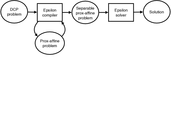
Figure 1: The Epsilon system: the compiler transforms a DCP-valid input problem into separable prox-affine problem to be solved by the solver. The prox-affine problem is also used as an intermediate representation internal to the compiler.

The main idea behind Epsilon is that instead of reducing general convex problems to conic form, we reduce them directly to a sum of prox-friendly functions composed with affine transformations and employ a large library of fast proximal and linear operator implementations to solve problems directly in this form. We call this intermediate representation the prox-affine form, and problems in this form can be directly mapped to a set of efficient proximal and linear operators available to the solver.

There are two main components of Epsilon: 1) the compiler, which transforms a DCP representation into a prox-affine form (and eventually a separable prox-affine form, to be discussed shortly), by a series of passes over the AST corresponding to the original problem; and 2) the solver, which solves the resulting problem using the fast implementation of these proximal and linear operators. An overview of the system is shown in Figure 1. This section describes each of these two components in detail.

3.1 The prox-affine form

The internal representation used by the compiler, as well as the input to the solver, is a convex optimization problem in prox-affine form

$$\operatorname*{minimize}_{x}\;\;\sum_{i=1}^{N}f_{i}(H_{i}(x)),\\$$ (8)

consisting of the sum of “prox-friendly” functions $f_{1},\ldots,f_{N}$ composed with a set of affine transformations $H_{1},\ldots,H_{n}$. In Epsilon, each $f_{i}\circ H_{i}$ is atomic meaning that it has a concrete numerical routine in the solver which implements the proximal operator for this function directly. The affine transformations are implemented with a library of linear operators which includes matrices (either sparse or dense), as well as more complex linear transformations like Kronecker products not easily represented as a single matrix, special cases like diagonal or scalar matrices and complex chains of multiple such linear transformations. Crucially, not every proximal operator can be combined with every linear operator, but it is the job of the Epsilon compiler, described shortly, to ensure that the problem is transformed to one where the compositions of proximal and linear operators have an available implementation. For example, very few proximal operators support composition with a general dense matrix (the sum-of-squares and subspace equality constraint being some of the only instances), but several can support composition with a diagonal matrix. Representing these distinctions in the Epsilon compiler is critical to deriving efficient proximal updates for the final optimization problems.

As an example of prox-affine form, the linear cone problem which forms the basis for existing disciplined convex programming systems (see Section 2.1),

$$\begin{split}\operatorname*{minimize}_{x}\;\;&c^{T}x\\ \operatorname*{subject\;to}\;\;&Ax=b\\ \;\;&x\in\mathcal{K},\end{split}$$ (9)

can be represented in prox-affine form as

$$\operatorname*{minimize}_{x}\;\;c^{T}x+I_{0}(Ax-b)+I_{\mathcal{K}}(x),$$ (10)

with $f_{1}$ being the identity function, $H_{1}$ being inner product with $c$, $f_{2}$ the indicator of the zero set, $H_{2}$ being the affine transformation $Ax-b$, $f_{3}$ the indicator of the cone $\mathcal{K}$ and $H_{2}$ the identity. Each of these functions is atomic and therefore has an efficient proximal operator; for example the proximal operator of $I_{0}(Ax-b)$ is simply the projection onto this subspace, and the proximal operator for $I_{\mathcal{K}}$ is the cone projection, and the proximal operator for $c^{T}x$ is simply $v-c$ (in fact, this term can be merged with one or both of the other terms and thus only two proximal operators are necessary). As the linear cone problem is thus a special case of prox-affine form, Epsilon enjoys the same generality as existing DCP systems.

In order to apply the operator splitting algorithm, we also define the separable prox-affine form

$$\begin{split}\operatorname*{minimize}_{x_{1},\ldots,x_{N}}\;\;&\sum_{i=1}^{N}f_{i}(H_{i}(x_{i}))\\ \operatorname*{subject\;to}\;\;&\sum_{i=1}^{N}A_{i}(x_{i})=b.\end{split}$$ (11)

which has separable objective and explicit additional linear equality constraints (which are required in order to guarantee that the objective can be made separable while remaining equivalent to the original problem). As above, the affine transformations $A_{i}$ are implemented by the linear operator library and can thus be represented with matrices or Kronecker products, as well as simpler forms such diagonal or scalar matrices. The latter are especially common in the separable form because they are often introduced for representing the consensus constraint that two variables be equal (e.g. $A_{i}=I$ or $A_{i}=-I$). Mathematically, there is little difference between the separable and non-separable forms; but computationally the separable form allows for direct application of the ADMM-based operator splitting algorithm. The separable prox-affine form can thus be mapped directly to a sequence of proximal and linear operator evaluations employed by the operator splitting algorithm.

The solution methods we present shortly for problems in separable prox-affine form will ultimately reduce to solving generalized proximal operators of the form

$$\operatorname{prox}_{f\circ H,A}(v)=\operatorname*{argmin}_{x}\lambda f(H(x))+(1/2)\|A(x)-v\|_{2}^{2}.$$ (12)

For most functions $f$ and affine transformations $H$ and $A$, this function will not have a simple closed-form solution, even if a simple proximal operator exists for $f$. The three important exceptions to this are when: 1) $f$ is the null function, 2) $f$ is the indicator of the zero cone, or 3) $f$ is a sum-of-squares function; in all these cases, the solution boils down to a linear least-squares problem. However, for certain linear operators (namely, scalar or diagonal transformations), there are many cases where the generalized proximal operator has a straightforward solution. A crucial element of the Epsilon compiler transformations is to produce a prox-affine form where the combination of $f$, $H$, and $A$ results in a solvable proximal operator; below, when we list the proximal operators supported by Epsilon, we will also specify which compositions with linear operators are valid.

3.2 Conversion to prox-affine form

Figure 2: Original abstract syntax tree for lasso $\|Ax-b\|_{2}^{2}+\lambda\|x\|_{1}$ (left) and converted to prox-affine form (right).

The first stage of the Epsilon compiler transforms an arbitrary disciplined convex problem into a prox-affine problem. Concretely, given an AST representing the optimization problem in its original form (which may consist of any valid composition of functions from the DCP library), this stage produces an AST with a reduced set of nodes:

• ADD. The sum of its children $x_{1}+\cdots+x_{n}$.

• PROX_FUNCTION. A prox-friendly function with proximal operator implementation in the Epsilon solver.

• LINEAR_MAP. A linear function with linear operator implementation in the Epsilon solver.

• VARIABLE, CONSTANT. Each leaf of the AST is either a variable or constant.

As such, once the AST is transformed into prox-affine form, each node corresponds to a function with a concrete proximal or linear operator implementation from the library of operators described in Section 4; an example of this transformation is shown in Figure 2.

Algorithm 1 Conversion of AST to prox-affine form

function ConvertProx($rules$, $tree$)

     $rule$ $\leftarrow$ MatchRule($rules$, $tree$)

     if $rule$ is nil then

         return ConvertConic($tree$)

     end if

     $args$, $indicators$ $\leftarrow$ ConvertProxArguments($rule$, $tree$)

     $output$ $\leftarrow$ CreateNode($rule$, $args$)

     for $indicator$ in $indicators$ do

         $output$ $\leftarrow$ Add($output$, ConvertProx($rules$, $indicator$))

     end for

     return $output$

end function

The transformation to prox-affine form is done in two passes over the AST representing the optimization problem. In the first pass, we convert all nodes representing linear functions to a nodes of type LINEAR_MAP which map directly to the linear operators available in the Epsilon solver. In terms of ASTs representing linear functions, there are two possibilities in any DCP-valid input problem: 1) direct linear transformaitons of inputs, such as the unary SUM or variable argument HSTACK and 2) binary functions such as MULTIPLY which apply a linear operator defined by a constant expression. The former have straightforward transformations to LINEAR_MAP representations; for the latter, DCP rules require that one of the arguments be constant and thus this argument is evaluated and converted to a linear operator (typically, a sparse, dense or diagonal matrix) and a LINEAR_MAP node with single argument.

In the second pass, we complete the transformation to prox-affine form by applying a set of prioritized rules, preferring to map ASTs onto a high-level proximal operator implementation when available but falling back to conic transformations, when necessary; the process is shown in Algorithm 1. In short, given an input tree (or subtree) along with a set of rules for proximal operator transformations, we match the input against these rules. If a matching proximal operator is found, we then transform the function arguments (represented by subtrees of the original input tree) so that they have valid form for composition with the proximal operator in question. In doing so, the process may introduce auxiliary variables and additional indicator functions; the behavior of ConvertProxArguments depends on the requirements of the particular proximal operator (see Section 4.2), but some common examples include:

• No-op. The expression $\max\{-x,0\}$ with variable $x$ is the hinge function $f(x)=\max\{x,0\}$, composed with the linear transformation $-I$. This represents a valid proximal operator so no further transformations are necessary and the argument $-x$ is returned as-is.

• Epigraph transformation. The expression $\|Ax-b\|_{1}$ with constants $A$, $b$ and variable $x$ matches a the proximal operator for the $\ell_{1}$-norm $\|\cdot\|_{1}$, but it cannot be composed with an arbitrary affine function given the set of proximal operators available in the Epsilon solver. Therefore, a new variable $y$ is introduced along with the constraint $I_{0}(Ax-b-y)$; $y$ is returned as argument, resulting in the new expression $\|y\|_{1}$.

• Kronecker product splitting. The expression $\|AXB-C\|_{F}^{2}$ with constants $A,B,C$ and variable $X$ matches the proximal operator for sum-of-squares, but evaluation would require factoring $F^{T}F+I$ where $F=B^{T}\otimes A$ which cannot be done efficiently given the linear operators available. Therefore, the compiler introduces a new variable $Z$, modifies the argument to be $\|AZ-C\|_{F}^{2}$ and introduces the constraint $I_{0}(XB-Z)$.

Once the arguments have been transformed to the proper form, CreateProx creates a PROX_FUNCTION node (with attribute specifying which proximal operator implementation) and the transformed arguments as children. Any indicators that were added by the argument conversion process are themselves recursively converted to prox-affine form and the result is accumulated in the output under an ADD node.

3.3 Optimization and separation of prox-affine form

Once the problem has been put in prox-affine form, the next stage of the compiler transforms it to be separable in preparation for the solver. As a given problem typically has many different separable prox-affine representations, this stage must balance the tradeoff between per-iteration computational complexity and the overall number of iterations that will be required to solve a given problem. As an extreme example, we can often split problems into a large number of proximal operators which are very cheap to evaluate but will require a large number of iterations. The theoretical analysis of convergence rates for operator splitting algorithms is an active area of research (see e.g. [4, 15, 9]) but Epsilon follows the simple philosophy of minimizing the total number of proximal operators in the separable form provided that each operator can be evaluated efficiently. This is implemented with multiple passes on the prox-affine form which split the problem as needed until it it satisfies the constraints required for applying the operator splitting algorithm described in Section 3.4.

Although we previously described the prox-affine form generically, where we were minimizing over a single variable $x$ and each term could potentially depend on all variable $f_{i}(H_{i}(x))$, the reality is that for many problems the $x$ variables are already “naturally” partitioned to some extent (for instance, this arises in epigraph transformations, where one function in the prox-affine form will only depend on epigraph variables). Thus, to be more concrete, we introduce a partitioning of the variables $x=(x_{1},\ldots,x_{k})$ (where here each $x_{j}$ is itself a vector of appropriate size, and let $\mathcal{J}_{i}$ denote the set of all variables that are used in the $i$th prox operator, i.e. our optimization problem becomes

$$\operatorname*{minimize}_{x_{1},\ldots,x_{k}}\;\sum_{i=1}^{n}f_{i}(H_{i}(x_{\mathcal{J}_{i}})).$$ (13)

The process of separation is effectively one of introducing “copies” of variables until we reach a point that each objective term $f_{i}$ has a unique set of variables, and the interactions between variables are captured entirely by the explicit equality constraints.

Given the form above, we describe the optimization problem via a bipartite graph, between nodes corresponding to objective functions $f_{1},\ldots,f_{N}$ (plus additional equality constraints, in the final form) and nodes corresponding to variables $x_{1},\ldots,x_{k}$. An edge exists between $f_{i}$ and $x_{j}$ if $j\in\mathcal{J}_{i}$, i.e. if the function uses that variable. By applying a sequence of transformations, we will introduce new variables and new equality constraints that will put the problem into a separable prox-affine form.

Definition of equivalence transformations.

Specifically, the compiler sequentially executes a series of transformations to put the problem in separable prox-affine form:

1. Move equality indicators. The first compiler stage (“Conversion to prox-affine form”, see Section 3.2) produces a single expression for the objective which includes all constraints via indicators; due to the nature of the transformations, many equality constraints are “simple” (e.g. involving $I$ or $-I$) and can thus be moved to actual constraints in the separable form. This pass performs these modifications based on the linear map associated with the edges corresponding to variables in each equality constraint, splitting expressions when necessary. For example, an objective term $I_{0}(Ax+y+z)$ is transformed to a new objective term $I_{0}(Ax-w)$ and the constraint $w+y+z=0$.

2. Combine objective terms. The basic properties of proximal operators (see e.g. [17]) allow simple functions like $c^{T}x$ and $\|x-b\|_{2}^{2}$ to be combined with other terms, reducing the number of proximal operators needed in the separable prox-affine form. This pass combines these terms assuming there is another objective term which includes the same variable.

3. Add variable copies and consensus constraints. The final pass guarantees that the objective is separable by introducing variable copies and consensus constraints. For example, the objective $f(x)+g(x)$ is transformed to $f(x_{1})+g(x_{2})$ and the constraint $x_{1}=x_{2}$ is added.

Figure 3: Compiler representation of prox-affine form as bipartite graph for $\exp(\|x\|_{2}+c^{T}x)+\|x\|_{1}$ after conversion pass (top, see equation 15) and after separation pass (bottom, see equation 16).

For illustration purposes, consider the problem

$$\operatorname*{minimize}_{x}\;\;\exp(\|x\|_{2}+c^{T}x)+\|x\|_{1}.$$ (14)

The first compiler stage converts this problem to prox-affine form by introducing auxiliary variables $t,s,v$, along with three cone constraints and two prox-friendly functions:

$$\operatorname*{minimize}_{x,t,s,v}\;\;\exp(t)+\|x\|_{1}+I_{\mathcal{Q}}(x,s)+I_{0}(s+c^{T}x-t-v)+I_{+}(v),$$ (15)

where $I_{\mathcal{Q}}$ denotes the indicator of the second-order cone, $I_{0}$ the zero cone and $I_{+}$ the nonnegative orthant. The problem in this form is the input for the second stage which constructs the bipartite graph shown in Figure 3 (top). The problem is then transformed to have separable objective with many of the terms in $I_{0}$ (those with simple linear maps) move to the constraint

$$\begin{split}\operatorname*{minimize}_{x_{1},x_{2},x_{3},t,s,v}\;\;&\exp(t)+\|x_{1}\|_{1}+I_{\mathcal{Q}}(x_{2},s)+I_{0}(c^{T}x_{3}-z)+I_{+}(v)\\ \operatorname*{subject\;to}\;\;&s+z-t-v=0\\ &x_{1}=x_{2}\\ &x_{2}=x_{3}\end{split}$$ (16)

and variables $x_{1},x_{2},x_{3}$ are introduced along with consensus constraints. The bipartite graph for the final output from the compiler, a problem in separable prox-affine form, is shown in Figure 3 (bottom).

3.4 Solving problems in prox-affine form

Once the problem has been put in separable prox-affine form, the Epsilon solver applies the ADMM-based operator splitting algorithm using the library of proximal and linear operators. The implementation details of each operator are abstracted from the high-level algorithm which applies the operators only through a common interface providing the basic mathematical operations required. Next we give a mathematical description of the operator splitting algorithm itself while the computational details of individual proximal and linear operators are discussed in Section 4.

The Epsilon solver employs a variant of ADMM to solve problems in the separable prox-affine form

$$\begin{split}\operatorname*{minimize}_{x_{i},\ldots,x_{N}}\;\;&\sum_{i=1}^{N}f_{i}(H_{i}(x_{i}))\\ \operatorname*{subject\;to}\;\;&\sum_{i=1}^{N}A_{i}(x_{i})=b.\end{split}$$ (17)

This approach can be motivated by considering the augmented Lagrangian

$$L_{\lambda}(x_{1},\ldots,x_{N},y)=\sum_{i=1}^{N}f_{i}(H(x_{i}))+y^{T}(Ax-b)+(1/2\lambda)\|Ax-b\|_{2}^{2}$$ (18)

where $y$ is the dual variable, $\lambda\geq 0$ is the augmented Lagrangian penalization parameter, and $Ax=\sum_{i=1}^{N}A_{i}(x_{i})$. The ADMM method applied here results in the Gauss-Seidel updates with

$$\begin{split}x_{i}^{k+1}&:=\operatorname*{argmin}_{x_{i}}\lambda f_{i}(H_{i}(x_{i}))+\frac{1}{2}\left\|\sum_{j<i}A_{j}(x_{j}^{k+1})+A_{i}(x_{i})+\sum_{j>i}A_{j}(x_{j}^{k})-b+u^{k}\right\|_{2}^{2}\\ u^{k+1}&:=u^{k}+Ax^{k+1}-b\end{split}$$ (19)

where we have $u=\lambda y$ is the scaled dual variable. Critically, the $x_{i}$-updates are applied using the (generalized) proximal operator, let

$$v_{i}^{k}=b-u^{k}-\sum_{j<i}A_{j}(x_{j}^{k+1})-\sum_{j>i}A_{j}(x_{j}^{k})$$ (20)

and we have

$$x_{i}^{k+1}:=\operatorname*{argmin}_{x_{i}}\lambda f_{i}(H_{i}(x_{i}))+(1/2)\|A(x_{i})-v_{i}^{k}\|_{2}^{2}=\operatorname{prox}_{\lambda f_{i}\circ H_{i},A_{i}}(v_{i}^{k})$$ (21)

The ability of the solver to evaluate the generalized proximal operator efficiently will depend on $f_{i}$ and $A_{i}$ (in the most common case $A_{i}^{T}A_{i}=\alpha I$, a scalar matrix, which can be handled by any proximal operator); it is the responsibility of the compiler to ensure that the prox-affine problem has been put in the required form such that these evaluations map to efficient implementations from the proximal operator library.

4 Fast atomic operators

The Epsilon solver contains a library of fast linear and proximal operators which implement the operations required for a high-level iterative algorithm such as the ADMM variant described in the previous section. In particular, the proximal operator library directly implements a large number of the functions available to disciplined convex programming frameworks reducing the need for extensive transformation before solving an optimization problem. As the evaluation of proximal operators as well as the operations required by high-level algorithms rely heavily on linear operators, Epsilon also provides a library of efficient linear operators (and a system for composing them), extending beyond the standard dense/sparse matrices typically found in generic convex solvers.

4.1 Linear operators

In general, the computation required for solving convex optimization often typically depends heavily on the application of linear operators. Most commonly these linear operators are implemented with sparse or dense matrices which explicitly represent the coefficients of the linear transformation. Clearly, in many cases this can be inefficient (see e.g. [5] and the references therein) and as such, we abstract the notion of a linear operator allowing for other implementations which can often be far more efficient than direct matrix representation.

A motivating example that arises in many applications is the use of matrix-valued variables. As intermediate representations for convex programming (both prox-affine and conic forms) typically reduce optimization problems over matrices to ones over vectors, matrix products naturally give rise to the Kronecker product. For example, consider the expression $AX$ where $A\in\mathbb{R}^{m\times n}$ is a dense constant and $X\in\mathbb{R}^{n\times k}$ is the optimization variable; we vectorize this product with $\operatorname*{vec}(AX)=(I\otimes A)\operatorname*{vec}(X)$ where $\otimes$ denotes the Kronecker product. Representing the Kronecker product as a sparse matrix is not only space inefficient (i.e. requiring $A$ to be repeated $k$ times) but can also be extremely costly to factor. In particular, the naive approach requires a sparse factorization of a $km\times kn$ matrix as opposed to factoring a dense $m\times n$ matrix $A$ directly. Explicitly maintaining the Kronecker product structure provides a mechanism for avoiding this unnecessary computational cost.

Epsilon augments the standard sparse/dense matrices with dedicated implementations for diagonal matrices, scalar matrices, the Kronecker product as well as composite types representing a sum or product:

• Dense matrix. A dense matrix $A\in\mathbb{R}^{m\times n}$ with $O(mn)$ storage.

• Sparse matrix. A sparse matrix $A\in\mathbb{R}^{m\times n}$ with O(# nonzeros) storage.

• Diagonal matrix. A diagonal matrix $A\in\mathbb{R}^{n\times n}$ with $O(n)$ storage.

• Scalar matrix. A scalar matrix $\alpha I\in\mathbb{R}^{n\times n}$ with $\alpha\in\mathbb{R}$ and $O(1)$ storage.

• Kronecker product. The Kronecker product of $A\in\mathbb{R}^{m\times n}$ and $B\in\mathbb{R}^{p\times q}$, representing a linear map $\mathbb{R}^{nq}\to\mathbb{R}^{mp}$ where $A$ and $B$ can themselves be any linear operator type.

• Sum. The sum of linear operators $A_{1}+\cdots+A_{N}$.

• Product. The product of linear operators $A_{1}\cdots A_{N}$.

• Abstract. An abstract linear operator which cannot be combined with any of the basic types. This is used to represent factorizations, see below.

Each linear operator type $A$ supports the following operations:

• Apply. Given a vector $x$, return $y=Ax$.

• Transpose. Return the linear operator $A^{T}$.

• Inverse. Return the linear operator $A^{-1}$.

The transpose operation returns a linear operator of the same type whereas the inverse operation may return a linear operator of a different type. The inverse operation is undefined for non-invertible linear operators and in practice is intended to be used in contexts where the linear transformation is known to be invertible.

In addition, linear operators also support binary operations for sum $A+B$ and product $AB$. This requires a system for type conversion, the basic rules for which are described with an ordering of the types corresponding to their sparsity ($Dense>Sparse>Diagonal>Scalar$); in order to combine any two of these types, we first promote the sparser type to to the denser type. For Kronecker products, type conversion depends on the arguments: the sum of two Kronecker products can be combined if one of the arguments is equivalent, e.g.

$$A\otimes B+A\otimes C=A\otimes(B+C)$$ (22)

while the product can be combined if the arguments have matching dimensions, i.e.

$$(A\otimes B)(C\otimes D)=AC\otimes BD$$ (23)

if we can form $AC$ and $BD$. In either case, if a combination is possible it will be performed along with the appropriate type conversion for the sum/product of the arguments themselves. If a combination is not possible according to these rules, the resulting type will instead be a $Sum$ or $Product$ composed of the arguments.

4.2 Proximal operators

The second class of operators that form the basis for Epsilon are the proximal operators, described above in Section 2.2. As seen in the resulting description of the ADMM algorithm, each individual solution over the $x_{i}$ variables can be represented via an operator

$$x^{k+1}_{i}:=\operatorname*{argmin}_{x_{i}}\lambda f(H(x_{i}))+\frac{1}{2}\|A_{i}(x_{i})-v_{i}^{k}\|^{2}_{2}$$ (24)

for some value of $v_{i}^{k}$ (which naturally depends generally on the dual variables for the equality constraints involving $x_{i}$ as well as the other $x_{j}$ variables). This is exactly the generalized proximal operator $x^{k+1}_{i}=\operatorname{prox}_{\lambda f\circ H_{i},A_{i}}(v)$. Indeed, the Epsilon compiler uses precisely the set of available fast proximal operators to reduce the convex optimization problems to fast forms relative to the corresponding cone problem; while any of the problems can be solved by reducing everything to these conic form (and thus using only proximal operators corresponding to cone projections), the speed of the solver crucially depends on the ability to evaluate a much wider range of these proximal operators efficiently.

It is well-known that many proximal operators have closed form solutions that can be solved much more quickly than general optimization problems (see e.g. [17] for a review). As the main goal of this current paper is not to develop new proximal operators, we merely highlight several of the operators included in Epsilon along with a general description of the methods used to solve them. The proximal operators group roughly into three categories: elementwise, vector, and matrix operators, for functions $f$ of scalar inputs, vector inputs, and matrix inputs respectively. Note that this is not a perfect division, because several vector matrix functions are simply sums of corresponding scalar functions, e.g., $\|x\|_{2}^{2}=\sum_{i=1}^{n}x_{i}^{2}$, but instead we use vector or matrix designations to refer to functions that cannot be decomposed over their inputs.

• Exact linear, quadratic, or cubic equations. Several prox operators can be solved using exact solutions to their gradient conditions. For instance, the prox operator of $f(x)=(ax-b)^{2}$ is given by the solution to the gradient equation $2a(ax-b)+x=0$, which is a simple linear equation. Similarly, the prox operators for $f(x)=-\log x$ and $f(x)=1/x$ have gradient conditions that are given by quadratic and cubic equations respectively. Here some care must be taken to ensure that we select the correct of two or three possible solutions, but this can be ensured analytically in many cases or simply by checking all solutions in the worst case. For vector functions, the proximal operator of a least-squares objective is also an instance of this case, though here of course the complexity requires a matrix inversion rather than a scalar linear equation.

• Soft thresholding. The absolute value and related functions can be solved via the soft thresholding operator. For example, the proximal operator of $f(x)=|x|$ is given by

  $$\operatorname{prox}_{\lambda f}(v)=\left\{\begin{array}[]{ll}v-\lambda&\mbox{ if }v>\lambda\\ 0&\mbox{ if }-\lambda\leq v\leq\lambda\\ v+\lambda&\mbox{ if }v<-\lambda.\end{array}\right.$$ (25)

• Newton’s method. Several proximal operators for smooth functions have no easily computed closed form solution. Nonetheless, in this case Newton’s method can be used to find a solution in reasonable time. For elementwise functions, for instance, these operations are relatively efficient, because in practice a very small number of Newton iterations are needed to reach numerical precision. For example, the proximal operator of the logistic function $f(x)=\log(1+\exp(x))$ has no closed form solution, but can easily computed with Newton’s method.

• Projection approaches. The proximal operator for several functions can be related to the projection on to a set. In the simplest case, the proximal operator for an indicator of a set is simply equal to the projection onto the set, giving prox operators for cone projections. However, additional proximal methods derive from Moreau decomposition [14], which states that

  $$v=\operatorname{prox}_{f}(v)+\operatorname{prox}_{f^{*}}(v)$$ (26)

  where $f^{*}$ denotes the Fenchel conjugate of $f$. For example, the proximal operator for the $\ell_{\infty}$-norm, $f(x)=\|x\|_{\infty}$ is given by

  $$\operatorname{prox}_{f}(v)=v-\mathcal{P}_{\|x\|_{1}\leq 1}(v)$$ (27)

  using the relation that the Fenchel conjugate of a normal is equal to the indicator of of the dual norm ball. The projection on to the $\ell_{1}$-ball can be accomplished in $O(n)$ time using a median of medians algorithm [8].

• Orthogonally invariant matrix functions. If a matrix input function is defined solely by the singular values (or eigenvalues) of a matrix, then the proximal operator can be computed using the singular value decomposition (or eigenvalue decomposition) of that matrix. Typically, the running time of these proximal operators are dominated by the cost of the decomposition itself, making them very efficient for reasonably-sized matrices. For example, the $\log\det$ function can be written as

  $$\log\det(X)=\sum_{i=1}^{n}\log\lambda_{i}$$ (28)

  so its proximal operator can be given by

  $$\operatorname{prox}_{\log\det}(X)=U\operatorname{prox}_{\log}(\Lambda)U^{T}$$ (29)

  where $\operatorname{prox}_{\log}(\Lambda)$ is shorthand for applying the proximal operator for the negative log function to each diagonal element of the eigenvalues $\Lambda$. The prox operator for the $\log$ function can itself be solved via a quadratic equation, so computing the inner prox term is only an $O(n)$ operation and the runtime is dominated by the $O(n^{3})$ cost of computing the eigenvalue decomposition.

• Special purpose algorithms. Finally, though we cannot enumerate these broadly, several proximal operators have special purpose fast solvers for these particular types of operators. A particularly relevant example is the fused lasso $f(x)=\|Dx\|_{1}$ where $D$ is the first order difference operator; this proximal operator can be solved efficiently via an $O(n)$ dynamic programming approach [12].

Function			Proximal operator
Category	Atom	Definition	Method	Complexity
Cone	Zero	$f(x)=I_{0}(Ax-b)$, $A\in\mathbb{R}^{m\times n}$	subspace projection	$O(mn^{2}+n^{3})$
	Nonnegative orthant	$f(x)=I_{+}(x)$	positive thresholding	$O(n)$
	Second-order cone	$f(x,t)=I_{\mathcal{Q}}(x,t)$, $x\in\mathbb{R}^{n}$, $t\in\mathbb{R}$	projection	$O(n)$
	Semidefinite cone	$f(X)=I_{\succeq}(X),X\in\mathbb{S}^{n}$	positive thresholding on $\lambda(X)$	$O(n^{3})$
Elementwise $x,y\in\mathbb{R}$	Absolute	$f(x)=|x|$	soft thresholding	$O(n)$
	Square	$f(x)=x^{2}$	linear equation	$O(n)$
	Hinge	$f(x)=\max\{x,0\}$	soft thresholding	$O(n)$
	Deadzone	$f(x)=\max\{|x|-\epsilon,0\},\;\epsilon\geq 0$	soft thresholding	$O(n)$
	Quantile	$f(x)=\max\{\alpha x,(\alpha-1)x\},\;0\leq\alpha\leq 1$	asymmetric soft thresholding	$O(n)$
	Logistic	$f(x)=\log(1+\exp(x))$	Newton	$O(n)\cdot(\mbox{\# Newton})$
	Inverse positive	$f(x)=1/x,\;x\geq 0$	Newton	$O(n)\cdot(\mbox{\# Newton})$
	Negative log	$f(x)=-\log(x),\;x\geq 0$	quadratic equation	$O(n)$
	Exponential	$f(x)=\exp(x)$	Newton	$O(n)\cdot(\mbox{\# Newton})$
	Negative entropy	$f(x)=x\cdot\log(x),\;x\geq 0$	Newton	$O(n)\cdot(\mbox{\# Newton})$
	KL Divergence	$f(x,y)=x\cdot\log(x/y),\;x,y\geq 0$	Newton	$O(n)\cdot(\mbox{\# Newton})$
	Quadratic over linear	$f(x,y)=x^{2}/y,\;y\geq 0$	cubic equation	$O(n)$
Vector $x\in\mathbb{R}^{n}$	$\ell_{1}$-norm	$f(x)=\|x\|_{1}$	soft thresholding	$O(n)$
	Sum-of-squares	$f(x)=\|Ax-b\|^{2}_{2}$, $A\in\mathbb{R}^{m\times n}$	normal equations	$O(mn^{2}+n^{3})$
	$\ell_{2}$-norm	$f(x)=\|x\|_{2}$	group soft thresholding	$O(n)$
	$\ell_{\infty}$-norm	$f(x)=\|x\|_{\infty}$	median of medians	$O(n)$
	Log-sum-exp	$f(x)=\log\left(\sum_{i=1}^{n}\exp(x_{i})\right)$	Newton	$O(n)\cdot(\mbox{\# Newton})$
	Fused lasso	$f(x)=\sum_{i=1}^{n-1}|x_{i}-x_{i+1}|$	dynamic programming [12]	$O(n)$
Matrix	Negative log det	$f(X)=-\log\det(X),X\in\mathbb{S}^{n}$	quadratic equation on $\lambda(X)$	$O(n^{3})$
	Nuclear norm	$f(X)=\|\sigma(X)\|_{1},X\in\mathbb{R}^{m\times n}$	soft thresholding on $\sigma(X)$	$O(n^{3})$
	Spectral norm	$f(X)=\|\sigma(X)\|_{\infty},X\in\mathbb{R}^{m\times n}$	median of medians on $\sigma(X)$	$O(n^{3})$

5 Examples and numerical results

In this section we present several examples of convex problems from statistical machine learning and compare Epsilon to existing approaches on a library of examples from several domains. At present, Python integration is provided (Matlab, R, Julia versions are planned) with CVXPY [6] providing the environment for constructing the disciplined convex programs and performing DCP validation. Epsilon effectively serves as a solver for CVXPY although behind the scenes the CVXPY/Epsilon interface is somewhat different than for other solvers as Epsilon compiler implements its own transformations on the AST. Nonetheless, from a user perspective problems are specified in the same syntax, a high-level domain specific language of which we give several examples in this section. Epsilon is open source and available at http://github.com/mwytock/epsilon/, including the code for all examples and benchmarks discussed here.

As Epsilon integrates with CVXPY, we make the natural comparison between Epsilon and the existing solvers for CVXPY which use the conic form. In particular, we compareEpsilon to ECOS [7], an interior point method and SCS [16], the “splitting conic solver”. In general, interior point methods achieve highly accurate solutions but have trouble scaling to larger problems and so it is unsurprising that Epsilon is able to solve problems to moderate accuracy several orders of magnitude faster than ECOS (this is also the case when comparing ECOS and SCS, see [16]). On the other hand, SCS employs an operator splitting method that is similar in spirit to the Epsilon solver, both being variants of ADMM; the main difference between the two is in the intermediate representation and set of available proximal operators: SCS solves the conic form produced by CVXPY with cone and subspace projections (using sparse matrices) while Epsilon solves the prox-affine form using the much larger library of fast proximal and linear operators described in Section 4. In practice, this has significant impact with Epsilon achieving the same level of accuracy as SCS an order of magnitude faster (or more) on many problems.

In what follows we examine several examples in detail followed by results on a library of 20+ problems common to applications in statistical machine learning and other domains. In the detailed examples, we start with a complete specification of the input problem (a few lines of Python in the CVXPY grammar), discuss the transformation by the Epsilon compiler to an abstract syntax tree representing a prox-affine problem and explore how the Epsilon solver scales relative to conic solvers. When printing the AST for individual problems, we adopt a concise functional form which is a serialized version of the abstract syntax trees shown in Figure 2 and is the internal representation of the Epsilon compiler, as well as input to the Epsilon solver.

5.1 Lasso

We start with the lasso problem

$$\operatorname*{minimize}_{\theta}\;\;(1/2)\|X\theta-y\|_{2}^{2}+\lambda\|\theta\|_{1},$$ (30)

where $X\in\mathbb{R}^{m\times n}$ contains input features, $y\in\mathbb{R}^{m}$ the outputs, and $\theta\in\mathbb{R}^{n}$ are the model parameters. The regularization parameter $\lambda\geq 0$ controls the tradeoff between data fit and sparsity in the solution—the lasso is especially useful in the high-dimensional case where $m\leq n$ as sparsity effectively controls the number of free parameters in the model, see [22] for details.

In CVXPY, the lasso can be written as

theta = Variable(n)
f = sum_squares(X*theta - y) + lam*norm1(theta)
prob = Problem(Minimize(f))

where sum_squares()/norm1() functions correspond directly to the two objective terms. In essence this problem is already in prox-affine form with proximal operators for $\|X\theta-y\|_{2}^{2}$ and $\|\theta\|_{1}$; thus the prox-affine AST produced by the Epsilon compiler merely adds an additional variable and equality constraint to make the objective separable:

objective:
  add(
    sum_squares(add(const(a), scalar(-1.00)*dense(B)*var(x))),
    norm1(var(y)))

constraints:
  zero(add(var(y), scalar(-1.00)*var(x)))

Note that in the automatically generated serialization of the AST, variable/constant names are auto-generated and do not necessarily correspond to user input. In this particular example a, B correspond to the constants $y$, $X$ from the original problem while x, y correspond to two copies of the optimization variable $\theta$.

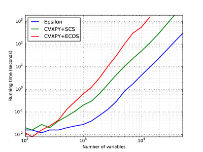
Figure 4: Comparison of running times on lasso example with dense $X\in\mathbb{R}^{m\times 10m}$.

Computationally, it is the evaluation of the sum-of-squares proximal operator which dominates the running time for Epsilon as it requires solving the normal equations. However, the cost of the factorization required is amortized as this step can be performed once before the first iteration of the algorithm, as discussed in Section 4.2. In Figure 4, we compare the running time of Epsilon to CVXPY+SCS/ECOS on a sequence of problems with dense $X\in\mathbb{R}^{m\times 10m}$. Epsilon (representing $X$ as a dense linear operator) performs a dense factorization while SCS embeds $X$ in a large sparse matrix and performs a sparse factorization (as it does with all problems). The difference in these factorizations explains the difference in running time as the time spent performing the actual iterations is negligible for both methods.

5.2 Multivariate lasso

In this example, we apply lasso to the multivariate regression setting where the output variable is now vector as opposed to a scalar in univariate regression. In particular,

$$\operatorname*{minimize}_{\Theta}\;\;(1/2)\|X\Theta-Y\|_{F}^{2}+\lambda\|\Theta\|_{1}$$ (31)

where $X\in\mathbb{R}^{m\times n}$ are input features, $Y\in\mathbb{R}^{m\times k}$ represent the $k$-dimensional response variable and the optimization variable is now a matrix $\Theta\in\mathbb{R}^{n\times k}$, representing the parameters of the multivariate regression model. The Frobenius norm $\|\cdot\|_{F}$ is the $\ell_{2}$-norm applied elementwise to a matrix and here $\|\cdot\|_{1}$ is also interpreted elementwise.

The CVXPY problem specification for the multivariate lasso is virtually identical to the standard lasso example

Theta = Variable(n,k)
f = sum_squares(X*Theta - Y) + lam*norm1(Theta)
prob = Problem(Minimize(f))

with the only change being the replacement of vectors y, theta with their matrix counterparts Y, Theta (by convention, we denote matrix-valued variables with capital letters). As a result, when the Epsilon compiler transforms this problem to the prox-affine AST,

objective:
  add(
    sum_squares(add(kron(scalar(1.00), dense(A))*var(X), scalar(-1.00)*const(B))),
    norm1(var(Y)))

constraints:
  zero(add(var(Y), scalar(-1.00)*var(X)))

the matrix-valued optimization variable results in the kron linear operator appearing as argument to the sum_squares proximal operator. This corresponds to the specialized Kronecker product linear operator implementation with (in this case) $O(mn)$ for the dense data matrix $X$.

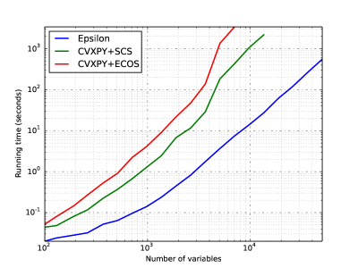
Figure 5: Comparison of running times on the multivariate Lasso example with dense $X\in\mathbb{R}^{m\times 10m}$ and $k=10$.

Although it is a simple to change to the problem specification to apply Lasso in the multivariate case, the new problem results in a substantially different computational running times for the solvers considered. In Figure 5 we show the running times of each approach on a sequence of problems with $X\in\mathbb{R}^{m\times 10m}$ and $Y\in\mathbb{R}^{m\times 10}$; where as on standard Lasso Epsilon was roughly 10x faster than SCS, now the gap is closer to 100x, e.g. for a problem with $1.35\times 10^{4}$ variables, SCS requires 2192 seconds vs. 27 seconds for Epsilon. The reason for this difference is due to the representation of the linear operator required for solving the normal equations for the least squares term

$$(1/2)\|(I_{k}\otimes X)\operatorname*{vec}(\Theta)-\operatorname*{vec}(Y)\|_{2}^{2}.$$ (32)

Since SCS is restricted to representing linear operators as sparse matrices, it must instantiate the Kronecker product explicitly (replicating the $X$ matrix $10$ times) and factor the resulting matrix with sparse methods. In contrast, Epsilon represents the Kronecker product directly (using the kron linear operator) and applies dense factorization methods without any unnecessary replication.

5.3 Total variation

In the previous lasso examples, we employ the $\ell_{1}$-norm to estimate a sparse set of regression coefficients—a natural extension to this idea is to incorporate a notion of structured sparsity. The fused lasso problem (originally proposed in [23])

$$\operatorname*{minimize}_{\theta}\;\;(1/2)\|X\theta-y\|_{2}^{2}+\lambda_{1}\|\theta\|_{1}+\lambda_{2}\sum_{i=1}^{n-1}\|\theta_{i+1}-\theta_{i}\|_{1}$$ (33)

employs total variation regularization (originally proposed in [20]) to encourage the differences of the coefficient vector $\theta_{i+1}-\theta_{i}$ to be sparse. Such structure naturally arises in problems where the dimensions of the coefficient vector correspond to vertices in a chain or grid, see e.g. [25, 1] for example applications.

For total variation problems, CVXPY provides a function tv() which makes the problem specification concise:

theta = Variable(n)
f = sum_squares(X*theta - y) + lam1*norm1(theta) + lam2*tv(theta)
prob = Problem(Minimize(f)).

In conic form this penalty is transformed to a set of a linear constraints which involve the first order differencing operator (to be defined shortly); however, Epsilon includes a direct proximal operator implementation of the total variation penalty and thus the compiler simply maps the problem specification onto three proximal operators

objective:
  add(
    least_squares(add(dense(C)*var(x), scalar(-1.00)*const(d))),
    norm1(var(y)),
    tv_1d(var(z)))

constraints:
  zero(add(var(z), scalar(-1.00)*var(y)))
  zero(add(var(z), scalar(-1.00)*var(x)))

with the addition of the necessary variable copies and equality constraints to make the objective separable.

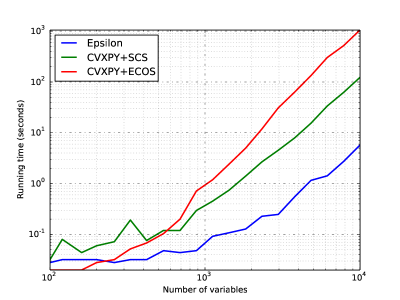
Figure 6: Comparison of running times on total variation example with $X\in\mathbb{R}^{m\times 10m}$, $y=X\theta_{0}+\epsilon$ with $\epsilon\sim\mathcal{N}(0,0.05^{2})$ where $\theta_{0}$ is piecewise constant with segments of length 10.

Figure 6 compares Epsilon to the conic solvers on a sequence of problems with $X\in\mathbb{R}^{m\times 10m}$. The main difference between the two approaches is that while Epsilon directly solves the proximal operator for the total variation penalty (using the dynamic programming algorithm of [12]), while transforming to conic form requires reformulating the fused lasso penalty as a linear program using auxiliary variables and involving the finite differencing operator $D\in\{-1,0,1\}^{(n-1)\times n}$

$$D=\left[\begin{array}[]{rrrrr}1&-1&0&\cdots\\ 0&1&-1&\cdots\\ 0&0&1&\cdots\\ \vdots&\vdots&\vdots&\ddots\\ \end{array}\right]$$ (34)

containing $1$ on the diagonal, $-1$ on the first super diagonal and 0 elsewhere. For even moderate $n$ this linear operator (which corresponds to the edge incidence matrix for the chain graph) is poorly conditioned which can be problematic for general solvers, see e.g. [19] for further details. The dedicated proximal operator avoids these issues, reducing running times—on a problem with $10^{4}$ variables, Epsilon requires $5.7$ seconds vs. $123$ seconds for SCS.

5.4 Library of convex programming examples

In this final section we present results on a library of example convex problems from statistical machine learning appearing frequently in the literature (e.g. [2, 16]). In general, each example depends on a variety of factors such as dimensions of the constants, data generation scheme and setting of the hyperparameters—we have chosen reasonable defaults for these settings. The complete specification for each problem is available in the the submodule epsilon.problems, distributed with the Epsilon code base. On each example, we run each solver considered using the default tolerances which for Epsilon and SCS correspond to moderate accuracy and high accuracy for ECOS. In practice, we observe that all solvers converge to a relative accuracy of $10^{-2}$ which is reasonable for the statistical applications under consideration.

	Epsilon		CVXPY+SCS		CVXPY+ECOS
Problem	Time	Objective	Time	Objective	Time	Objective
basis_pursuit	1.35s	$1.44\times 10^{2}$	17.26s	$1.45\times 10^{2}$	217.68s	$1.45\times 10^{2}$
covsel	0.93s	$3.74\times 10^{2}$	25.09s	$3.73\times 10^{2}$	-	-
fused_lasso	3.87s	$7.46\times 10^{1}$	57.85s	$7.41\times 10^{1}$	641.34s	$7.41\times 10^{1}$
hinge_l1	3.71s	$1.15\times 10^{3}$	45.59s	$1.15\times 10^{3}$	678.47s	$1.15\times 10^{3}$
hinge_l1_sparse	14.26s	$1.38\times 10^{3}$	106.75s	$1.38\times 10^{3}$	183.65s	$1.38\times 10^{3}$
hinge_l2	3.58s	$3.87\times 10^{3}$	133.10s	$3.87\times 10^{3}$	1708.31s	$3.87\times 10^{3}$
hinge_l2_sparse	1.82s	$8.08\times 10^{3}$	28.40s	$8.09\times 10^{3}$	47.72s	$8.08\times 10^{3}$
huber	0.20s	$2.18\times 10^{3}$	3.17s	$2.18\times 10^{3}$	28.43s	$2.18\times 10^{3}$
lasso	3.69s	$3.21\times 10^{1}$	20.54s	$3.21\times 10^{1}$	215.68s	$3.21\times 10^{1}$
lasso_sparse	13.58s	$4.37\times 10^{2}$	56.94s	$4.37\times 10^{2}$	277.80s	$4.37\times 10^{2}$
least_abs_dev	0.10s	$7.09\times 10^{3}$	2.96s	$7.10\times 10^{3}$	11.46s	$7.09\times 10^{3}$
logreg_l1	3.70s	$8.18\times 10^{2}$	51.60s	$8.18\times 10^{2}$	684.86s	$8.17\times 10^{2}$
logreg_l1_sparse	6.69s	$9.61\times 10^{2}$	33.35s	$9.63\times 10^{2}$	310.02s	$9.61\times 10^{2}$
lp	0.33s	$7.77\times 10^{2}$	3.78s	$7.75\times 10^{2}$	7.58s	$7.77\times 10^{2}$
mnist	0.91s	$1.75\times 10^{3}$	219.63s	$1.72\times 10^{3}$	1752.97s	$1.72\times 10^{3}$
mv_lasso	7.14s	$4.87\times 10^{2}$	824.83s	$4.88\times 10^{2}$	-	-
qp	1.39s	$4.30\times 10^{3}$	3.20s	$4.28\times 10^{3}$	23.12s	$4.24\times 10^{3}$
robust_pca	0.59s	$1.71\times 10^{3}$	2.88s	$1.71\times 10^{3}$	-	-
tv_1d	0.13s	$2.29\times 10^{5}$	51.85s	$2.95\times 10^{5}$	-	-

Table 1: Comparison of running time and objective value between Epsilon and CVXPY with SCS and ECOS solvers, a value of “-” indicates a lack of result either due to solver failure, unsupported problem or 1 hour timeout.

The running times in Table 1 show that on all problem examples considered, Epsilon is faster than SCS and ECOS and often by a wide margin. In general, we observe that Epsilon tends to solve problems in fewer ADMM iterations and for many problems the iterations are faster due in part to operating on a smaller number of variables. There are numerous reasons for these differences, some of which we have explored in the more detailed examples appearing earlier in this section.

6 Conclusions

We have discussed Epsilon, a new system for general convex programming based on representing any disciplined convex problem as a sum of functions with fast proximal operators. The central idea is that by retaining more of the original problem structure with a richer intermediate representation (the prox-affine form), we achieve more efficient solution methods. This is inspired in part by the recent surge of popularity in operator splitting methods leading to a very large number of “specialized” algorithms which ultimately can be reduced to a particular sequence of proximal operator invocations. In short, Epsilon seeks to automate this process by providing a large library of proximal (and linear) operators as well as a compiler to transform any DCP-valid problem into a separable prox-affine form for direct solution by an ADMM-based algorithm. Crucially, the iterative algorithm is agnostic to the details of the operators and thus the system can be extended by adding new operator implementations and the corresponding rules to the Epsilon compiler. Each new proximal operator that is added to the Epsilon system in this fashion reduces the need for laborious specialized implementations to solve a single problem. Ultimately, an interesting direction for future work is thus the further development of Epsilon and other tools toward automating many of the mechanical transformations and other tasks required by convex programming practitioners to develop efficient algorithms and deploy them on data at scale.

References

- [1] Samrachana Adhikari, Fabrizio Lecci, James T Becker, Brian W Junker, Lewis H Kuller, Oscar L Lopez, and Ryan J Tibshirani. High-dimensional longitudinal classification with the multinomial fused lasso. arXiv preprint arXiv:1501.07518, 2015.
- [2] Stephen Boyd, Neal Parikh, Eric Chu, Borja Peleato, and Jonathan Eckstein. Distributed optimization and statistical learning via the alternating direction method of multipliers. Foundations and Trends® in Machine Learning, 3(1):1–122, 2011.
- [3] Stephen Boyd and Lieven Vandenberghe. Convex optimization. Cambridge university press, 2004.
- [4] Damek Davis and Wotao Yin. Convergence rate analysis of several splitting schemes. arXiv preprint arXiv:1406.4834, 2014.
- [5] Steven Diamond and Stephen Boyd. Convex optimization with abstract linear operators. 2015.
- [6] Steven Diamond and Stephen Boyd. CVXPY: A Python-embedded modeling language for convex optimization. 2015.
- [7] Alexander Domahidi, Eric Chu, and Stephen Boyd. Ecos: An socp solver for embedded systems. In Control Conference (ECC), 2013 European, pages 3071–3076. IEEE, 2013.
- [8] John Duchi, Shai Shalev-Shwartz, Yoram Singer, and Tushar Chandra. Efficient projections onto the l 1-ball for learning in high dimensions. In Proceedings of the 25th international conference on Machine learning, pages 272–279. ACM, 2008.
- [9] Pontus Giselsson. Tight global linear convergence rate bounds for douglas-rachford splitting. arXiv preprint arXiv:1506.01556, 2015.
- [10] Michael Grant, Stephen Boyd, and Yinyu Ye. Disciplined convex programming. Springer, 2006.
- [11] Michael Grant, Stephen Boyd, and Yinyu Ye. CVX: Matlab software for disciplined convex programming, 2008.
- [12] Nicholas A Johnson. A dynamic programming algorithm for the fused lasso and l 0-segmentation. Journal of Computational and Graphical Statistics, 22(2):246–260, 2013.
- [13] Johan Löfberg. YALMIP: A toolbox for modeling and optimization in matlab. In Computer Aided Control Systems Design, 2004 IEEE International Symposium on, pages 284–289. IEEE, 2004.
- [14] Jean-Jacques Moreau. Fonctions convexes duales et points proximaux dans un espace hilbertien. CR Acad. Sci. Paris Sér. A Math, 255:2897–2899, 1962.
- [15] Robert Nishihara, Laurent Lessard, Benjamin Recht, Andrew Packard, and Michael I Jordan. A general analysis of the convergence of admm. arXiv preprint arXiv:1502.02009, 2015.
- [16] Brendan O’Donoghue, Eric Chu, Neal Parikh, and Stephen Boyd. Operator splitting for conic optimization via homogeneous self-dual embedding. arXiv preprint arXiv:1312.3039, 2013.
- [17] Neal Parikh and Stephen Boyd. Proximal algorithms. Foundations and Trends in optimization, 1(3):123–231, 2013.
- [18] Florian A Potra and Stephen J Wright. Interior-point methods. Journal of Computational and Applied Mathematics, 124(1):281–302, 2000.
- [19] Aaditya Ramdas and Ryan J Tibshirani. Fast and flexible admm algorithms for trend filtering. arXiv preprint arXiv:1406.2082, 2014.
- [20] Leonid I Rudin, Stanley Osher, and Emad Fatemi. Nonlinear total variation based noise removal algorithms. Physica D: Nonlinear Phenomena, 60(1):259–268, 1992.
- [21] Ernest K Ryu and Stephen Boyd. Primer on monotone operator methods. 2015.
- [22] Robert Tibshirani. Regression shrinkage and selection via the lasso. Journal of the Royal Statistical Society. Series B (Methodological), pages 267–288, 1996.
- [23] Robert Tibshirani, Michael Saunders, Saharon Rosset, Ji Zhu, and Keith Knight. Sparsity and smoothness via the fused lasso. Journal of the Royal Statistical Society: Series B (Statistical Methodology), 67(1):91–108, 2005.
- [24] Madeleine Udell, Karanveer Mohan, David Zeng, Jenny Hong, Steven Diamond, and Stephen Boyd. Convex optimization in julia. In High Performance Technical Computing in Dynamic Languages (HPTCDL), 2014 First Workshop for, pages 18–28. IEEE, 2014.
- [25] Bo Xin, Yoshinobu Kawahara, Yizhou Wang, and Wen Gao. Efficient generalized fused lasso and its application to the diagnosis of alzheimer’s disease. In Twenty-Eighth AAAI Conference on Artificial Intelligence, pages 2163–2169, 2014.