Normally Hyperbolic Invariant Laminations and diffusive behaviour for the generalized Arnold example away from resonances

Abstract

In this paper we study existence of Normally Hyperbolic Invariant Laminations (NHIL) for a nearly integrable system given by the product of the pendulum and the rotator perturbed with a small coupling between the two. This example was introduced by Arnold [1]. Using a separatrix map, introduced in a low dimensional case by Zaslavskii-Filonenko [61] and studied in a multidimensional case by Treschev and Piftankin [51, 52, 55, 56], for an open class of trigonometric perturbations we prove that NHIL do exist. Moreover, using a second order expansion for the separatrix map from [27], we prove that the system restricted to this NHIL is a skew product of nearly integrable cylinder maps. Application of the results from [11] about random iteration of such skew products show that in the proper $\varepsilon$-dependent time scale the push forward of a Bernoulli measure supported on this NHIL weakly converges to an Ito diffusion process on the line as $\varepsilon$ tends to zero.

1 The main result

Consider the following nearly integrable Hamiltonian system:

$$\begin{aligned} H_{\varepsilon}(p,q,I,\varphi,t)=H_{0}(p,q,I)+\varepsilon H_{1}(p,q,I,\varphi,t):=\qquad\qquad\qquad\qquad\\ =\underbrace{\dfrac{\ \ I^{2}\ \ }{2}}_{rotor}+\underbrace{\dfrac{p^{2}}{2}+(\cos q-1)}_{pendulum}+\varepsilon H_{1}(p,q,I,\varphi,t),\end{aligned}$$ (1)

where $q,\varphi,t\in\mathbb{T}$ are angles, $p,I\in\mathbb{R}$ (see Fig. 1). In the case $H_{1}=(\cos q-1)(\cos\varphi+\cos t)$ this example was proposed by Arnold [1].

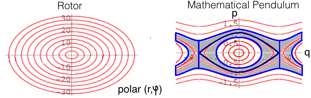
Figure 1: The rotor times the pendulum

For $\varepsilon=0$ we have a direct product of the rotor $\{\dot{\theta}=I,\ \dot{I}=0\}$ and the pendulum $\{\dot{q}=p,\ \dot{q}=\sin q\}$. We shall study dynamics of this systems when the $(p,q)$-component is near the separatrices $\dfrac{p^{2}}{2}+(\cos q-1)=0$. Perturbations of systems, given by the product of the rotor and an integrable system with a separatrix loop, are called apiori unstable. Since they were introduced by Arnold [1], they recieved a lot of attention both in mathematics, astronomy, and physics community, see e.g. [2, 7, 13, 14, 15, 16, 12, 18, 20, 21, 25, 37, 39, 41, 53, 57, 58]. It also inspired a variety of examples with instabilities, see e.g. [4, 5, 6, 9, 19, 22, 26, 30, 31, 32, 33, 40, 42, 43, 44, 45, 47].

Numerical experiments and heuristic arguments proposed by Chirikov and his followers indicate that if we choose many initial conditions so that the $(p,q)$-component is close to $(p,q)=0$ and integrate solutions over $\sim\varepsilon^{-2}\ln 1/\varepsilon$-time, the outcome is that the $r$-displacement behaives stochastically, where the randomness comes from initial conditions. This is the reason Chirikov called this phenomenon Arnold diffusion.

1.1 Random fluctuations of eccentricity in Kirkwood gaps in the asteroid belt

A similar diffusive behavior was observed numerically in many other nearly integrable problems. To give another illustrative example consider motion of asteroids in the asteroid belt. The asteroid belt is located between orbits of Mars and Jupiter and has around one million asteroids of diameter of at least one kilometer. When astromoters build a histogram based on orbital perioid of asteroids there are well known gaps called Kirkwood gaps. These gaps occur when ratio of Jupiter and of an asteroid is a rational with small denominator: $3:1,5:2,7:3$ (see Fig. 2). This correspond to so called mean motion resonances for the three body problem. Wisdom [59] made a numerical analysis of dynamics at mean motion resonance and observed random jumps of eccentricity of asteroids for $3:1$ resonances. Later similar behavior was observed for $5:2$ resonance. For other resonances, following the mechanism from [22], one could expect that eccentricity has random fluctuations and as they accumulate eccentricity reaches a certain critical value an orbit of asteroid starts to cross the orbit of Mars. This eventually leads either to a collision with Mars, or capture by Mars, or a close encounter (see also [49]). The latter changes the orbit so drastically that almost certainly it disappears from the asteroid belt. In [22] in the $3:1$ Kirkwood gap and small Jupiter’s eccenricity we prove existence of certain orbits whose eccentricity change by $0.32$ for the restricted planar three body problem.

Figure 2: The distribution of Asteroids in the asteroid belt and Kirkwood gaps

1.2 Diffusion processes and infinitesimal generators

In order to formalize the statement about diffusive behavior we need to recall some basic probabilistic notions. A random process $\{W_{t},t\geq 0\}$ called the Wiener process or a Browninan motion if the following four conditions hold:

$B_{0}=0$, $B_{t}$ is almost surely continuous, $B_{t}$ has independent increments, $B_{t}-B_{s}\sim\mathcal{N}(0,t-s)$ for any $0\leq s\leq t$, where $\mathcal{N}(\mu,\sigma^{2})$ denotes the normal distribution with expected value $\mu$ and variance $\sigma^{2}$.

The condition that it has independent increments means that if $0\leq s_{1}\leq t_{1}\leq s_{2}\leq t_{2}$, then $B_{t_{1}}-B_{s_{1}}$ and $B_{t_{2}}-B_{s_{2}}$ are independent random variables.

A Brownian motion is a properly chosen limit of the standard random walk. A generalization of a Brownian motion is a diffusion process or an Ito diffusion. To define it let $(\Omega,\Sigma,P)$ be a probability space. Let $X:[0,+\infty)\times\Omega\to\mathbb{R}$. It is called an Ito diffusion if it satisfies a stochastic differential equation of the form

$$\mathrm{d}X_{t}=b(X_{t})\,\mathrm{d}t+\sigma(X_{t})\,\mathrm{d}B_{t},$$ (2)

where B is an Brownian motion and $b:\mathbb{R}\to\mathbb{R}$ and $\sigma:\mathbb{R}\to\mathbb{R}$ are the drift and the variance respectively. For a point $x\in\mathbb{R}$, let $\mathbf{P}^{x}$ denote the law of $X$ given initial data $X_{0}=x$, and let $\mathbf{E}^{x}$ denote expectation with respect to $\mathbf{P}^{x}$.

The infinitesimal generator of $X$ is the operator $A$, which is defined to act on suitable functions $f:\mathbb{R}\to\mathbb{R}$ by

$$Af(x)=\lim_{t\downarrow 0}\dfrac{\mathbf{E}^{x}[f(X_{t})]-f(x)}{t}.$$

The set of all functions $f$ for which this limit exists at a point $x$ is denoted $D_{A}(x)$, while $D_{A}$ denotes the set of all $f$’s for which the limit exists for all $x\in\mathbb{R}$. One can show that any compactly-supported $C^{2}$ function $f$ lies in $D_{A}$ and that

$$Af(x)=b(x)\dfrac{\partial f}{\partial x}+\dfrac{1}{2}\sigma(x)\dfrac{\partial^{2}f}{\partial x\partial x}.$$

In particular, we can characterize a diffusion process by the drift $b(x)$ and the variance $\sigma(x)$. Thus, we can identify an Ito diffusion if we know the drift $b(x)$ and the variance $\sigma(x)$.

1.3 Conjecture on rotor’s stochastic diffusive behavior

Consider the Hamiltonian $H_{\varepsilon}$ of the form (1). Let $\mathbb{A}=\mathbb{R}\times\mathbb{T}$ be a $2$-dimensional annulus, and $B^{2}_{\sqrt{\varepsilon}}(0)$ be the ${\sqrt{\varepsilon}}$-ball around the origin in $\mathbb{A}\ni(p,q)$, and $B_{\varepsilon}(I^{*})$ be an $\varepsilon$-neighborhood of $I^{*}$ in $\mathbb{R}$. Let $X=(p,q,I,\varphi,t)$ denote a point in the whole phase space and by $X_{t}^{\varepsilon}$ the time $t$ map of $H_{\varepsilon}$ with $X$ as the initial condition. Pick any $I^{*}\in\mathbb{R}$. Denote by $\mu^{\varepsilon}(I^{*})$ the normalized Lebesgue measure supported inside

$$D_{\varepsilon}(I^{*}):=B^{2}_{\sqrt{\varepsilon}}(0)\times B_{\varepsilon}(I^{*})\times\mathbb{T}^{2}\ni(p,q,I,\varphi,t).$$

Denote by $\mu^{\varepsilon}_{t}$ the image of $\mu^{\varepsilon}(I^{*})$ under the time $t$ map of $H_{\varepsilon}$, by $\Pi_{I}$ the projection onto the $I$-component, by $t_{\varepsilon}=-\frac{\ln\varepsilon}{\varepsilon^{2}}$ the rescaled time.

Conjecture 1.1.

Let the initial distribution be the normalized Lebesgue measure $\mu^{\varepsilon}(I^{*})$ for some $I^{*}$. Then for a generic perturbation $\varepsilon H_{1}(\cdot)$ there are smooth functions $b(I)$ and $\sigma(I)>0$, depending on $H_{1}$ and $H_{0}$ only, such that for each $s>0$ and $\,t_{\varepsilon}=s\,\varepsilon^{-2}\log\frac{1}{\varepsilon}$ the distribution $\Pi_{I}(\phi^{t_{\varepsilon}}_{*}\mu^{\varepsilon})$ converges weakly, as $\varepsilon\to 0$, to the distribution of $I_{s}$, where $I_{\bullet}$ is the diffusion process with the drift $b$ and the variance $\sigma$, starting at $I_{0}=I^{*}$.

This conjecture can be viewed as formalization of the discussion in chapter 7 of [15]. As a matter of fact presence of a possible drift in not mentioned there. In this paper Chirikov coined the term for this instability phenomenon — Arnold diffusion.

Remark 1.1.

The strong form of this conjecture is to find a family of measures $\mu^{\varepsilon}$ such that for some $c>0$

$$\lim_{\varepsilon\to 0}\ \dfrac{\text{Leb }(\text{supp }\mu^{\varepsilon})}{\text{Leb }(B^{2}_{\sqrt{\varepsilon}}(0)\times B_{\varepsilon}(I_{0})\times\mathbb{T}^{2})}>0,$$

where Leb is the $5$-dimensional Lebesgue measure. In other words, the conditional probability to start $\varepsilon$-close to the unstable equilibria of the pendulum and action $r_{0}$ and exhibit stochastic diffusive behavior is uniformly positive.

In [34] we give numerical evidence in favour of this conjecture. Here is the description of numerical experiments in [34]. Let $\varepsilon=0.01$ and $T=\varepsilon^{-2}\ln 1/\varepsilon$. On Figure 3 we present several histograms plotting displacement of the $I$-component after time $T,\,2T,\,4T,\,8T$ with 6 different groups of initial conditions. Each group has of $10^{6}$ points. In each group we start with a large set of initial conditions close to $p=q=0,\ I=I^{*}$.

1.4 Statement of the Main Result

In this paper we study a simplified versions of $H_{\varepsilon}$ in (1). Namely, we consider the following family of perturbations

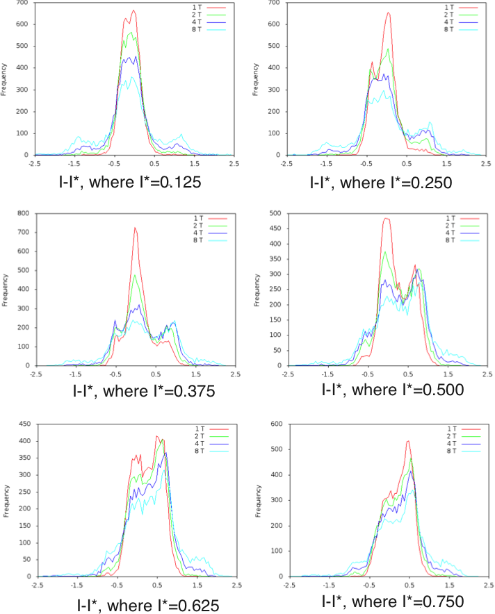
Figure 3: Histograms of the $I$-dispacement

$$H_{\varepsilon}(p,q,I,\phi,t)=\dfrac{I^{2}}{2}+\dfrac{p^{2}}{2}+(\cos q-1)+\varepsilon P_{N}(\exp(iq),\exp(i\varphi),\exp(it)),$$ (3)

where $P_{N}(\exp(iq),\exp(i\varphi),\exp(it))$ is a real valued trigonometric polynomial, i.e. for some $N\geq 2$ and real coefficients $p^{\prime}_{k_{1},k_{2},k_{3}}$ and $p^{\prime\prime}_{k_{1},k_{2},k_{3}}$ with $|k_{i}|\leq N,i=1,2,3$ we have

$$\begin{aligned} P_{N}(\exp(iq),\exp(i\varphi),\exp(it))=&\\ \sum_{|k_{i}|\leq N,i=1,2,3}p^{\prime}_{k_{1},k_{2},k_{3}}\cos(k_{1}q+k_{2}\varphi+k_{3}t)&+p^{\prime\prime}_{k_{1},k_{2},k_{3}}\sin(k_{1}q+k_{2}\varphi+k_{3}t).\end{aligned}$$ (4)

In the example proposed by Arnold [1] we have $P_{2}=(1-\cos q)(\cos\varphi+\cos t)$.

Denote by $\mathbb{R}^{m(N)}$ the space of real coefficients of $P_{N}$ and by $\phi^{t}$ the time $t$ map of the Hamiltonian vector field of $H_{\varepsilon}$. Let

$$\mathcal{N}_{\beta}(P_{N})=\{k\in\mathbb{Z}^{3}:(p^{\prime}_{k},p^{\prime\prime}_{k})\neq 0\}$$

and

$$\mathcal{N}_{\beta}^{(2)}(P_{N})=\{k\in\mathbb{Z}^{3}:k=k_{1}+k_{2},k_{1},k_{2}\in\mathcal{N}_{\beta}(P_{N})\}.$$

Fix $\beta>0$. Define a $\beta$-non-resonant domains

$$\mathcal{D}_{\beta}(P_{N})=\{I\in\mathbb{R}:\forall k\in\mathcal{N}_{\beta}^{(2)}(P_{N})\ \text{we have }\ |k_{2}I+k_{3}|\geq\beta\}.$$ (5)

Notice that $\mathcal{D}_{\beta}(P_{N})$ contains the subset of $\mathbb{R}$ with $\beta$-neighborhoods of all rational numbers $p/q$ with $0<|q|\leq 2N$ removed. Here $N$ is degree of $P_{N}$. Let $I^{*}\in\mathcal{D}_{\beta}(P_{N})$ and $X^{*}=(p,q,I^{*},\varphi,t)$. Denote

$$\widetilde{\phi}^{t}X^{*}=\begin{cases}\phi^{t}X^{*}\qquad\qquad\ &\text{if}\ \Pi_{I}(\phi^{s}X^{*})\in\mathcal{D}^{(2)}_{\beta}(P_{N})\ \text{ for all }\ 0<s\leq t.\\ \widetilde{\phi}^{t}X^{*}=\phi^{t^{*}}X^{*}\ &\text{if}\ \Pi_{I}(\phi^{s}X^{*})\in\mathcal{D}^{(2)}_{\beta}(P_{N})\text{ for }0<s<t^{*}\\ &\&\ \Pi_{I}(\phi^{t^{*}}X^{*})\in\partial\mathcal{D}^{(2)}_{\beta}(P_{N}).\end{cases}$$ (6)

Theorem 1.2.

For the Arnold’s example (3–4) there is an open set of trigonometric polynomials $P_{N}$ and smooth functions $b(I)$ and $\sigma(I)$, depending on $P_{N}$ only, such that:

for each $\beta,s>0$ and each $I^{*}\in\mathcal{D}^{(2)}_{2\beta}(P)$ there exists a probability measure $\mu^{\varepsilon}$, supported in $D_{\varepsilon}(I^{*})$, with the property that for $\,t_{\varepsilon}=s\,\varepsilon^{-2}\log\frac{1}{\varepsilon}$ the distribution $\Pi_{I}(\widetilde{\phi}^{t_{\varepsilon}}_{*}\mu^{\varepsilon})$ converges weakly, as $\varepsilon\to 0$, to the distribution of $I_{\min\{s,\tau\}}$, where $I_{\bullet}$ is the diffusion process with the drift $b(I)$ and the variance $\sigma(I)$, starting at $I_{0}=I^{*}$, and $\tau$ is the first time that the process $I_{\bullet}$ reaches the boundary $\partial\mathcal{D}^{(2)}_{\beta}(P)$.

The proof of this Theorem consists of three steps:

1. (A separatrix map) Write a separatrix map $\mathcal{SM}_{\varepsilon}$ for the generalized Arnold example (3–4). First, the map $\mathcal{SM}_{\varepsilon}$ is defined for general an apriori unstable systems in section 2 and computed for this example in Corollary 2.5. One can view the separatrix map as an induced return map of the time one map $\phi^{1}$ of $H_{\varepsilon}$ into a carefully chosen fundamental domain (see Fig. 4).

   

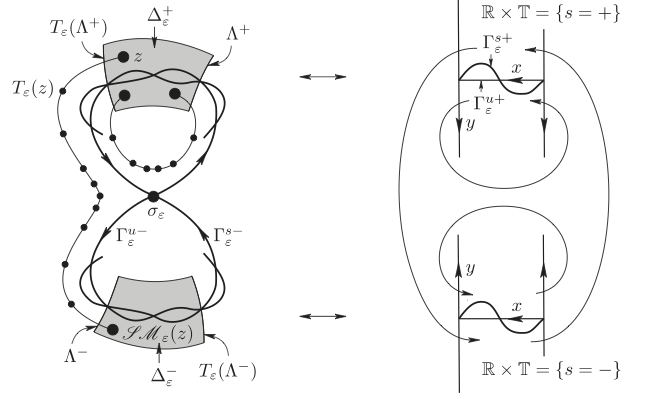
   Figure 4: The fundamental domain $\Delta_{\varepsilon}^{\pm}$

2. (Isolating block and Normally Hyperbolic Laminations (NHIL)) In Appendix A using Conley’s idea of isolating block (see e.g. [3, 46]) we derive a sufficient condition for existence of a NHIL and in section 3, after a careful analysis of the separatrix map and its linearization, we verify this sufficient condition and construct a NHIL ${\bf\Lambda}_{\varepsilon}$. Leaves of this NHIL ${\bf\Lambda}_{\varepsilon}$ are $2$-dimensional cylinders.

3. (A skew product of cylinder maps) In section 4, using results from [27], we find coordinates such that the restricted system $\mathcal{SM}_{\varepsilon}|_{{\bf\Lambda}_{\varepsilon}}:{\bf\Lambda}_{\varepsilon}\to{\bf\Lambda}_{\varepsilon}$ has the following skew-product form of maps of a cylinder $\mathbb{A}=\mathbb{R}\times\mathbb{T}\ni(R,\theta)$

   $$\begin{aligned} R^{*}=R+\varepsilon\log\varepsilon\cdot N^{[\omega]_{k}}_{1}\left(\theta,\small{\frac{R}{\log\varepsilon}}\right)+\varepsilon^{2}\log\varepsilon\cdot N^{[\omega]_{k}}_{2}\left(\theta,\small{\frac{R}{\log\varepsilon}}\right)+\mathcal{O}_{\omega}(\varepsilon^{3})|\log\varepsilon|\\ \theta^{*}=\theta+R+\mathcal{O}_{\omega}(\varepsilon\log\varepsilon).\qquad\qquad\qquad\qquad\qquad\qquad\qquad\qquad\qquad\qquad\ \quad\end{aligned}$$ (7)

   where $\omega_{i}=0$ or $1,$ and $\omega=(\dots,\omega_{i},\dots)\in\{0,1\}^{\mathbb{Z}}$, $N^{[\omega]_{k}}_{i},\ i=1,2$ are smooth functions, depending on only finite terms of $\omega$, i.e. $[\omega]_{k}=(\omega_{-k},\cdots,\omega_{0},\cdots,\omega_{k})$ and both remainder terms depend on $\omega$. See Corollary 4.6. This model fits into the framework of [11].

1.5 Possible extensions of Theorem 1.2.

• (Extension to the whole $\mathbb{R}$) We hope to extend our results to the whole $\mathbb{R}$, i.e. to neighborhood of rationals $p/q$ with $|q|\leq N$. The difficulties are of purely technical nature. For $I$ in the $\beta$-non-resonant domain $\mathcal{D}^{(2)}_{\beta}(P)$ in [27] we show that the separatrix map $\mathcal{SM}_{\varepsilon}$ has a relatively simple expression (see Theorem 4.1) In the $\beta$-resonant domain $\mathbb{R}\setminus\mathcal{D}^{(2)}_{\beta}(P)$ we also compute the separatrix map $\mathcal{SM}_{\varepsilon}$ with high accuracy, but the corresponding expression is more involved (see Theorem 3.4, section 2 [27]). However, this leads to a skew product of cylinder maps not covered by [11]. It seems feasible that technique developped in [11] still applies.

• (Generic trigonometric perturbations) Even though it seems plausible, at the moment we are not able to construct a NHIL for a generic trigonometric perturbations. Our pertubations are close to purely time dependent perturbations, namely, $H_{1}(q,\varphi,t)=(\cos q-1)f(t)+ag(q,\varphi,t)$, where $f,g$ are trigonometric polynomials, $f(t)$ satisfies some nondegeneracy condition and $a$ is sufficiently small (see condition (24)).

• (Generic smooth/analytic perturbations) At the moment our scheme uses trigonometric nature of the perturbations in a very essential way. In this setting we can divide the fundamental region $\Delta$ into the $\beta$-resonant and the $2\beta$-non-resonant zones (see definition (5)). In general, this definition is combersome. However, in [18] this problem is treated for generic smooth perturbations.

  Removing this trigonometricity assumption leads to considerable technical difficulties.

  1. The second order expansion of the separatrix map [27] has to be redone.

  2. Derivation of the skew product model of maps of the cylinder from section 4 has to be worked out in that setting.

  3. For a new skew product one needs to adapt the technique from [11].

1.6 Remarks on Theorem 1.2.

• Notice that the Hamiltonian $H_{\varepsilon}$ in (3) has a $3$-dimensional normally hyperbolic invariant cylinder, denoted $\Lambda_{\varepsilon}$, near the cylinder $\Lambda_{0}:=\mathbb{R}\times\mathbb{T}^{2}=\{p=q=0\}$ (see section C for definitions). The orbits we study always stay close to stable (resp. unstable) $W^{s}(\Lambda_{\varepsilon})$ (resp. $W^{u}(\Lambda_{\varepsilon})$) manifold of $\Lambda_{\varepsilon}$. Naturally, the dynamics of each such an orbit can be decomposed into “loops” starting and ending near $\Lambda_{0}$.

• A measure $\mu^{\varepsilon}$ can be chosen so that $\Pi_{I}(\mu^{\varepsilon})$ is the $\delta$-measure at $I^{*}$. The support of supp $\mu^{\varepsilon}$ belongs to a NHIL ${\bf\Lambda}_{\varepsilon}$ constructed in section 3.

• The NHIL ${\bf\Lambda}_{\varepsilon}$ is “located” near two connected components of intersections of stable & unstable manifolds $W^{s}(\Lambda_{\varepsilon})$ and $W^{u}(\Lambda_{\varepsilon})$ resp. of the NHIC $\Lambda_{\varepsilon}$.

• Locally ${\bf\Lambda}_{\varepsilon}$ is a prodict of a $3$-dimensional cylinder $\mathbb{A}^{3}=\mathbb{R}\times\mathbb{T}\times\mathbb{T}$ and a Cantor set $\Lambda_{\varepsilon}$. This Cantor set is homeomorphic to $\Sigma=\{0,1\}^{\mathbb{Z}}$.

• $\mu^{\varepsilon}$ can be chosen as a Benoulli measure on ${\bf\Lambda}_{\varepsilon}\cap\{(I,\varphi,t)=(I^{*},\varphi^{*},t^{*})\}$ for some $(I^{*},\varphi^{*},t^{*})$ in the domain of definition, which is homeomorphic to $\Sigma$.

• Since $\mu^{\varepsilon}$ is supported on the NHIL, Lebesgue measure of its support is zero.

• Notice that such a lamination is not invariant, it is weakly invariant in the following sense: Let ${\bf\Lambda}_{\varepsilon}\cap\{I\in\mathcal{D}_{\beta}(P)\}$. Then if $X\in{\bf\Lambda}_{\varepsilon}$ and $I\in\mathcal{D}_{\beta}(P)$, then $\phi^{1}(X)\in{\bf\Lambda}_{\varepsilon}\cap\{I\in\mathcal{D}_{\beta/2}(P)\}$. Indeed, $\beta$ is independent of $\varepsilon$. In other words, the only way orbits can escape from ${\bf\Lambda}_{\varepsilon}$ is through the top (resp. bottom) boundary given by intersections with $\partial\mathcal{D}_{\beta}(P)$.

• An open set $U\subset\mathbb{R}^{m(N)}$ of validity of this theorem is stated in terms of an associated Poincaré-Melnikov integral (or splitting potentials) $M(I,\varphi,t)$ (see section 2.4). See also comments in the previous section 1.5 about extensions to general trigonometric perturbations.

Here is a detailed plan of the proof and of structure of the paper:

• Computation of a separatrix map $\mathcal{SM}_{\varepsilon}$:

  • Write a general separatrix map $\mathcal{SM}_{\varepsilon}$ (section 2.1);

  • Derive a specific form of $\mathcal{SM}_{\varepsilon}$ for the generalized Arnold example (section 2.2);

  • The map $\mathcal{SM}_{\varepsilon}$ involves the splitting potential, which is computed in section 2.3;

  • Properties of the splitting potential are analysed in section. 2.4

• Analysis of the linearization of the separatrix map and construction of a normally hyperbolic invariant lamination (NHIL):

  • We state the main existence theorem of NHILs in section 3.1;

  • We start the proof of this Theorem by analyzing the linearization of the separatrix map $\mathcal{SM}_{\varepsilon}$ in section 3.2;

  • In section 3.3 we compute almost fixed cylinders $\mathcal{SM}_{\varepsilon}(C_{i})\approx C_{i},i=0,1$ and almost period two cylinders $\mathcal{SM}_{\varepsilon}(C_{01})\approx C_{10},\ \mathcal{SM}_{\varepsilon}(C_{10})\approx C_{01}$. These cylinders serve as centers of the isolating blocks.

  • In section 3.4 we construct isolating blocks and present cone fields on them, then proved the [C1-C5] conditions defined in Appendix A.

• In section 4 we derive a skew product of cylinder maps model (7). This consists of two steps.

  • In section 4.1 we state a result from [27] about the expansion of the separatrix map up to the second order in actions.

  • In section 4.2 on each of cylindric leaves of the NHIL ${\bf\Lambda}_{\varepsilon}$ we introduce a concervative coordinates and derive the random cylinder map model (7).

• In Appendix A we state a sufficient condition of existence of a NHIL, which essentially goes back to Conley (see e.g. [46]);

• In Appendix C we define normally hyperbolic invariant laminations and skew products.

• In Appendix D we state the result from [11] about weak convergence to a diffusion process for distributions of the vertical component of random iterations of cylinder maps (7).

• In Appendix E we study certain classes of exact nearly integrable maps of a cylinder. This is used in derivation of the random cylinder map model (7) in section 4.2.

Acknowledgement The authors would like to warmly thank Marcel Guardia for many useful discussions of analytic aspects of this work. Comments of Leonid Polterovich on symplectic structure of normally hyperbolic laminations led to a special normal form from section 4.2 and is a significant step in the proof. Remarks of Leonid Koralov, Dmitry Dolgopyat, Anatoly Neishtadt, Amie Wilkinson were useful for this project. The authors warmly thank to all these people. The first author acknowledges partial support of the NSF grant DMS-1402164.

2 A separatrix map of apriori unstable systems

Consider a Hamiltonian system

$$H_{\varepsilon}(p,q,I,\varphi,t)=H_{0}(p,q,I)+\varepsilon H_{1}(p,q,I,\varphi,t),$$

where $H_{0}(p,q,I)=H_{0}(0,0,I)$ has two separatrix loops. Denote by $\mathcal{D}_{0}$ any bounded region. For example, $H_{0}$ is the harmonic oscillator times the pendulum:

$$H_{0}(p,q,I)=\dfrac{I^{2}}{2}+\dfrac{p^{2}}{2}+(\cos q-1),$$

where $p,I\in\mathbb{R}$ are actions and $q,\varphi\in\mathbb{T}$ are angles. We can use formula (1.10) in Piftankin-Treschev with $n=1$ and no $\varepsilon^{2}$-term. In order to apply results of this paper impose the following conditions:

• The function $H$ is $C^{r}$–smooth with respect to $(I,\varphi,p,q,t)$, where $r\geq 13$.

  We consider the alternative assumption.

• The function $H_{0}$ is $C^{r}$ for $r\geq 50$ and $H$ is $C^{s}$-smooth in all arguments for $s\geq 6$ and $r\geq 8s+2$.

Notice that regularity of $H_{0}$ exceeds that one of $H_{1}$. The more regular $H_{0}+\varepsilon H_{1}$, the better estimates of the remainder terms of the separatrix map we have. For a $C^{1}$ analysis of the separatrix map, it would suffice $s\geq 5$ and $r\geq 42$, $r\geq 8s+2$.

• For any $r\in\mathcal{D}_{0}$ the function $H_{0}(I_{0},p,q)$ has a non-degenerate saddle point $(p,q)=(p_{0},q_{0})$. Every point $(p_{0},q_{0})$ belongs to a compact connected component of the set

  $$\{(p,q)\in\text{Fig}_{\bf 8}:H_{0}(I_{0},p,q)=H_{0}(I_{0},p_{0},q_{0})\}.$$

  Moreover, $(p_{0},q_{0})$ is the unique critical point of $H_{0}(I_{0},p,q)$ on this component (see Fig. 5).

Remark 2.1.

Using Prop.1, [56], if one assumes that the saddle is at a certain point $(p,q)=(p^{0},q^{0})$ which depends smoothly on $I$, then, one can perform a symplectic change of coordinates so that the critical point is at $(p,q)=(0,0)$ for all $I\in\mathcal{D}$. After such a coordinate change $C^{r}$ in H1 is replaced by $C^{r-2}$.

The point $(p_{0},q_{0})\in$ Fig₈ depends smoothly on $I_{0}$ and is a hyperbolic equilibrium point of a system with one degree of freedom and with Hamiltonian $H_{0}(I_{0},p,q)$. The corresponding separatrices are doubled and form a curve of figure-eight type. Below we denote the loops of the figure-eight by $\widehat{\gamma}^{\pm}(I_{0})$, where $\widehat{\gamma}^{+}(I_{0})$ is called the upper loop and $\widehat{\gamma}^{-}(I_{0})$ — the lower loop. The loops $\widehat{\gamma}^{\pm}(I_{0})$ have a natural orientation generated by the flow of the system. The orientation on Fig₈ is determined by the system of coordinates $p,q$.

Notice that in our case these loops do not depend on $r_{0}$. To satisfy [H2] consider the cylinder $\mathbb{A}=\mathbb{R}\times\mathbb{T}\ni(p,q)$ and a diffeomorphism from the set $|\frac{p^{2}}{2}+(\cos q-1)|\leq 0.1$ to the figure-eight.

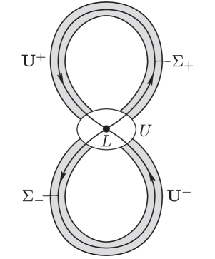
Figure 5: Separatrices in the form of the figure-eight

• For any $I_{0}\in\mathcal{D}_{0}$ the natural orientation of $\widehat{\gamma}^{\pm}(I_{0})$ coincides with the orientation of the domain Fig₈, i.e.the motion along the separatrices is counterclockwise (see Fig. 5).

• The variables $I$ are separated from $p$ and $q$ in the non-perturbed Hamiltonian, i.e. $H_{0}(I,p,q)=F(I,f(p,q)))$.

Both [H3] and [H4] are clearly satisfied for the generalized example of Arnold (3–4).

Now we define the separatrix map from [52] describing the dynamics of the systems satisfying assumptions [H1-H4]. As an intermediate step it is also convenient to study perturbations vanishing on the cylinder $\Lambda_{0}$:

$$H_{1}(p,q,I,\varphi,t):=(\cos q-1)P(\exp(i\varphi),\,\exp(it)),$$ (8)

where $P$ is a real valued trigonometric polynomial.This is a particular case of triginometric polynomials of the form (4). For the classical Arnold example [1] we have $P=\cos\varphi+\cos t$.

2.1 Formulas of the separatrix map of a priori unstable systems

We would like to apply Theorem 6.1 from Piftankin-Treschev [52] presenting almost explicit formulas with a remainder for the separatrix map. It uses the Poincaré-Melnikov potential for the “outer” dynamics and the restriction of the perturbation to $(p,q)=0$ for the “inner” dynamics. The words “inner” dynamics is used to describe dynamics of the Hamiltonian flow restricted to the normally hyperbolic invariant cylinder $\Lambda$ and the “outer” dynamics to describe evolution along invariant manifolds of $\Lambda$.

Consider the frequency map $\nu(I)=\partial_{I}H_{0}(0,0,I)=I$ as the map $\nu:\mathcal{D}_{0}\to\mathbb{R}^{n}$. It gives the frequency of the torus $\mathcal{T}(I):=\{(0,0,I)\}$. Let $\phi:\mathbb{R}\to[0,1]$ be a $C^{\infty}$-smooth function such that $\phi(I)=0$ for $|I|\geq 1$ and $\phi(I)=1$ for $|I|<1/2$. Fix some $\delta\in(0,1/4]$. In (6.1–6.2) Piftankin-Treschev chapter 6 §2 they introduce an auxiliary Hamiltonian

$$\begin{aligned} \overline{\bf H}_{1}(I,\varphi,t)&=&\sum_{(k,k_{0})\in\mathbb{Z}^{2}}\phi\left(\dfrac{k\varphi+k_{0}}{\varepsilon^{\delta}}\right)H^{k,k_{0}}_{1}(I)\exp(2\pi\,i(k\varphi+k_{0}t)),\\ {\bf H}_{1}(I,\varphi)\ \ &=&\bar{\bf H}(I,\varphi,0),\qquad\qquad\qquad\qquad\qquad\qquad\qquad\qquad\end{aligned}$$ (9)

where $H^{k,k_{0}}_{1}(I)$ are Fourier coefficients of $H_{1}(0,0,I,\varphi,t)$. The function $\overline{\bf H}_{1}$ is the mollified mean of $H_{1}(0,0,I,\varphi,t)$ along the non-perturbed trajectories on the tori $\mathcal{T}(I)$. This procedure is similar to local averaging proposed in [3], Thms 3.1, 3.2. This function tends pointwise to the usual average as $\varepsilon\to 0$

$$\sum_{kI+k_{0}=0}H^{k,k_{0}}_{1}(I)\exp(2\pi i(k\varphi+k_{0}t))=\lim_{T\to\infty}\dfrac{1}{T}\int_{0}^{T}H_{1}(0,0,I,\varphi+\nu(I)\,s,t+s)\,ds.$$

Since averaged are discontinuous in $I$ we prefer to deal with ${\bf H}_{1}$ and $\overline{\bf H}_{1}$. For the generalized Arnold example these functions vanish.

Let $\mathcal{D}\subset\mathcal{D}_{0}$ be an open connected domain with compact closure $\overline{\mathcal{D}}$. Let ${\bf K}$ be a compact set in $\mathbb{R}^{n+1}$. In the spaces $C^{r}(\overline{\mathcal{D}}\times{\bf K})$ we introduce the following norms: for $f\in C^{r}(\overline{\mathcal{D}}\times{\bf K})$ let

$$\|f(r,z)\|_{r}^{(b)}=\max_{0\leq l^{\prime}+l^{\prime\prime}\leq r}b^{l^{\prime}}\left|\dfrac{\partial^{l^{\prime}+l^{\prime\prime}f}}{\partial r^{l^{\prime}}\partial z_{1}^{l_{1}^{\prime\prime}}\dots\partial z_{m}^{l_{m}^{\prime\prime}}},\right|$$

where $l^{\prime\prime}=l_{1}^{\prime\prime}+\dots+l_{m}^{\prime\prime}$. It is assumed that $f$ can take values in $\mathbb{R}^{s}$, where $s$ is an arbitrary positive integer. The norms $\|\cdot\|^{b}_{r}$ are anisotropic, and the variables $r$ play a special role in these norms because the additional factor $b$ corresponds to the derivatives with respect to $r$. Obviously, $\|\cdot\|^{1}_{r}$ is the usual $C^{r}$-norm. This norm is similar to a skew-symmetric norm introduced in [35], section 7.2. The same definition applies to functions periodic in $z$, i.e. $z\in\mathbb{T}^{n+1}$.

For brievity denote

$$\|\cdot\|_{r}^{*}=\|\cdot\|_{r}^{(\varepsilon^{\delta})}.$$ (10)

For functions $f\in C^{r}(\overline{\mathcal{D}}\times\bf K)$ and $g\in C^{0}(\overline{\mathcal{D}}\times\bf K)$ we say that

$$f=O^{(b)}_{0}(g)\ \textup{ if }\ \|f\|_{r}^{(b)}\leq C\,g^{k},$$

where $C$ does not depend on $b$. For brevity we write

$$\|\cdot\|_{r}^{*}=\|\cdot\|_{r}^{(\varepsilon^{\delta})},\ \ \ O^{(b)}=O^{(b)}_{1},\ \ \ O^{*}_{k}=O^{(\varepsilon^{\delta})}_{k}$$ (11)

Notice that for the generalized Arnold example we have $n=1,\ E(r)=\frac{r^{2}}{2}$.

Theorem 2.2.

For the Hamiltonian $H_{\varepsilon}$ there are smooth functions

$$\lambda,\kappa^{\pm}:\bar{\mathcal{D}}\to\mathbb{R},\ M^{\pm}:\bar{\mathcal{D}}\times\mathbb{T}^{2}\to\mathbb{R},$$

a constant $c>0$ and coordinates $(\eta,\xi,h,\tau)$ such that the following conditions hold:

• $\omega=d\eta\wedge d\xi+dh\wedge d\tau$;

• $\eta=I+O^{*}(\varepsilon^{3/4},H_{0}-E(r)),\xi+\nu(I)\,\tau=q+f$, where the function $f$ depends only on $(p,I,\varphi,\varepsilon)$ and is such that $f(I,0,0,0)=0,\ h=H_{0}+O^{*}(\varepsilon^{3/4},H_{0}-E(I))$, and $H_{0}=H_{0}(p,q,I).$ Let

  $$w_{0} := h^{+}-E(\eta^{+})-\varepsilon{\bf H}(\eta^{+},\xi+\nu(\eta^{+})\tau,t),$$ (12)

  where $w_{0}$ measures distance to the invariant manifolds.

• For any $(\eta^{+},\xi,h^{+},\tau)$ such that

  $$\begin{aligned} c^{-1}\,\varepsilon^{5/4}\,|\log\varepsilon|<|w_{0}|<c\,\varepsilon^{7/8},\ \qquad\qquad\\ |\tau|<c^{-1},\qquad c<|w_{0}|\exp(\lambda(\eta^{+})t^{+})<c^{-1},\end{aligned}$$ (13)

  the map $g^{t^{+}}_{\varepsilon}T^{t^{+}}_{\varepsilon}=\mathcal{SM}_{\varepsilon}$ at time $t^{+}$ is defined as follows:

  $$\mathcal{SM}_{\varepsilon}(\eta,\xi,h,\tau,s,t^{+})=(\eta^{+},\xi^{+},h^{+},\tau^{+},s^{+}),$$

  where

  $$\begin{aligned} \eta^{+}&=&\eta-\varepsilon M^{\sigma}_{\xi}(\eta^{+},\xi,\tau)-\dfrac{\partial_{\xi}w_{0}}{\lambda}\log\left|\dfrac{\kappa^{\sigma}w_{0}}{\lambda}\right|+{\bf O}_{2}\ \\ \xi^{+}&=&\xi+\varepsilon M^{\sigma}_{\eta}(\eta^{+},\xi,\tau)+\dfrac{\partial_{\eta^{+}}w_{0}}{\lambda}\log\left|\dfrac{\kappa^{\sigma}w_{0}}{\lambda}\right|+{\bf O}_{1}\\ h^{+}&=&h-\varepsilon M^{\sigma}_{\tau}(\eta^{+},\xi,\tau)-\dfrac{\partial_{\tau}w_{0}}{\lambda}\log\left|\dfrac{\kappa^{\sigma}w_{0}}{\lambda}\right|+{\bf O}_{2}\ \\ \tau^{+}&=&\tau+t^{+}+\ \qquad\qquad\dfrac{\partial_{h^{+}}w_{0}}{\lambda}\log\left|\dfrac{\kappa^{\sigma}w_{0}}{\lambda}\right|+{\bf O}_{1}\ \\ \sigma^{+}&=&\sigma\text{ sgn }w.\quad\qquad\qquad\qquad\qquad\qquad\qquad\end{aligned}$$ (14)

where $\lambda,\nu,$ and $\kappa^{\sigma}$ are functions of $\eta^{+}$ and $t^{+}$ is an integer such that

$$\left|\tau+t^{+}+\dfrac{\partial_{h^{+}}w_{0}}{\lambda}\log\left|\dfrac{\kappa^{\sigma}w_{0}}{\lambda}\right|\right|<c^{-1}$$ (15)

$${\bf O}_{1}=O^{(\varepsilon^{1/4})}(\varepsilon^{7/8})\log\varepsilon,\quad{\bf O}_{2}=O^{(\varepsilon^{1/4})}(\varepsilon^{5/4})\log^{2}\varepsilon.$$

The superscript $\sigma$ fixes the separatrix loop passed along by the trajectory.

Remark 2.3.

For $t^{+}$ satisfying (15) the separatrix map is given by

$$\eta=\mathcal{S}_{\xi},\quad\xi^{+}=\mathcal{S}_{\eta^{+}},\quad h=\mathcal{S}_{\tau},\quad\tau^{+}=t^{+}+\mathcal{S}_{h^{+}},\quad\sigma^{+}=\sigma\cdot\text{sgn }w_{0},$$

where the generating function $\mathcal{S}$ has the form

$$\mathcal{S}(\eta^{+},\xi,h^{+},\tau,s,t^{+})=\eta^{+}\xi+h^{+}\tau+\varepsilon\Theta^{\sigma}(\eta^{+},\xi,\tau)+\frac{w_{0}}{\lambda}\log\left|\dfrac{\kappa^{\sigma}w_{0}}{\lambda e}\right|+O^{*}(\varepsilon^{9/8})\log^{2}\varepsilon.$$

Notice that the map $\mathcal{S}$ depends on $t^{+}$ only via the last term.

2.2 Parameters of the separatrix maps for the generalized Arnold example

Notice that for the Arnold’s example the unperturbed Hamiltonian is given by a direct product of $(I,\varphi)$ and $(p,q)$ variables: $H_{0}=\frac{I^{2}}{2}+\frac{p^{2}}{2}+(\cos q-1).$ Using explicit formulas for $\lambda,\kappa^{\pm}$ and $M^{\pm}$ in Section 6 §[52] we compute them.

The functions $\lambda>0$, $\kappa^{\pm}>0$ and $\mu^{\pm}\in\mathbb{R}$ are defined by the unperturbed Hamiltonian $H_{0}$ as follows. Hypothesis H2 implies that both eigenvalues of the matrix

$$\Lambda(I)=\begin{pmatrix}-\partial_{pq}H_{0}(I,0,0)&-\partial_{qq}H_{0}(I,0,0)\\ \partial_{pp}H_{0}(I,0,0)&\partial_{pq}H_{0}(I,0,0)\end{pmatrix}$$ (16)

are real and the trace of this matrix is equal to 0 for all $I$. We denote by $\lambda(I)$ the positive eigenvalue of this matrix.

Let $\gamma^{\pm}(I,\cdot):\mathbb{R}\to\{(p,q)\in\text{Fig}_{\bf 8}:H_{0}(I_{0},p,q)=H_{0}(I_{0},0,0)\}$ be the natural parametrizations of the separatrix loops $\widehat{\gamma}^{\pm}(r)$, i.e.

$$\dot{\gamma}^{\pm}(y,t)=(-\partial_{q}H_{0}(I,\gamma^{\pm}(t)),\partial_{p}H_{0}(I,\gamma^{\pm}(t)))$$

and $a_{\pm}=a_{\pm}(I)$ be the left eigenvectors of $A$, i.e.

$$a_{+}A=\lambda a_{+},\qquad a_{-}A=\lambda a_{-}.$$

such that the $2\times 2$ matrix with rows $a_{+}$ and $a_{-}$ has unit determinant.

In Proposition 6.3 [52] there are explicit formulas for $\kappa^{\pm}(I)$, given as integrals of $a_{+}$ along $\gamma^{\pm}$. In the case that the separatrix loops $\widehat{\gamma}^{\pm}(I)$ are independent of $I$ we have that $\kappa^{\pm}$ are also independent of $I$ (see formulas (6.13–6.14)).

The natural parametrizations on $\widehat{\gamma}^{\pm}$ are determined up to a time shift $t\mapsto t+\phi_{\pm}(I)$. Natural parametrizations are said to be compatible if they depend smoothly on $I$ and

$$\lim_{t\to-\infty}\frac{\langle a_{+}(I),\gamma^{+}(I,t)\rangle}{\langle a_{+}(I),\gamma^{-}(I,t)\rangle}=-1.$$

Compatible parametrizations are determined up to a simultaneous shift, namely, if $\gamma^{+}(I,t^{+}(I,t)),\gamma^{-}(I,t^{-}(I,t))$ is another pair of compatible parametrizations, then $t^{+}(I,t)=t^{-}(I,t)=t-t_{0}(I)$ with a smooth function $t_{0}$.

If a solution of the non-perturbed system belongs to $\Gamma^{\pm}(I)$, it has the form

$$\begin{aligned} (I,\varphi,p,q)(t)&=\Gamma^{\sigma}(I,\xi,\tau+t),\qquad\xi\in\mathbb{T},\ \tau\in\mathbb{R},\ \sigma\in\{+,-\},\\ &\Gamma^{\sigma}(I,\xi,\tau)=(I,\xi+\nu(I)\tau,\gamma^{\sigma}(I,\tau)).\qquad\qquad\quad\end{aligned}$$ (17)

Let

$$H^{\sigma}_{*}(I,\xi,\tau,t)=H_{1}(\Gamma^{\sigma}(I,\xi,\tau),t-\tau)-H_{1}(I,\xi+\nu t,0,0,t-\tau).$$

The functions $H^{\sigma}_{*}(I,\xi,\tau,t)$ vanishes as $t\to\pm\infty$.

Proposition 2.4.

Suppose that the parametrizations $\gamma^{\pm}$ are compatible. Then

$$M^{\sigma}(I,\xi,\tau)=-\int_{-\infty}^{\infty}H^{\sigma}_{*}(I,\xi,\tau,t)dt.$$

The functions $M^{\sigma}$ are called splitting potentials. They are 1-periodic with respect to $\xi$ and $\tau$. We proved the following

Corollary 2.5.

For the generalized Arnold example (3) with trigonometric perturbations of the form (8) there are constants $\kappa^{\pm},c>0,$ and $\lambda>0$ such that for $w=h^{+}-E(\eta^{+})$ satisfying $c^{-1}\varepsilon^{2}<|w|<c\varepsilon^{7/8}$ the separatrix map $\mathcal{SM}_{\varepsilon}$ has the form

$$\begin{aligned} \eta^{+}&=&\eta-\varepsilon M^{\sigma}_{\xi}(\eta^{+},\xi,\tau)\ \qquad\qquad\qquad\quad+{\bf O}_{2}\\ \xi^{+}&=&\xi+\varepsilon M^{\sigma}_{\eta^{+}}(\eta^{+},\xi,\tau)-\dfrac{\eta^{+}}{\lambda}\log\left|\dfrac{\kappa^{\sigma}w}{\lambda}\right|+{\bf O}_{1}\\ h^{+}&=&h-\varepsilon M^{\sigma}_{\tau}(\eta^{+},\xi,\tau)\quad\qquad\qquad\quad\quad+{\bf O}_{2}\\ \tau^{+}&=&\tau+t^{+}+\quad\qquad\qquad\frac{1}{\lambda}\ \log\left|\dfrac{\kappa^{\sigma}w}{\lambda}\right|+{\bf O}_{1}\\ \sigma^{+}&=&\sigma\text{ sgn }w,\quad\qquad\qquad\qquad\qquad\qquad\qquad\end{aligned}$$ (18)

where

$${\bf O}_{1}=O^{*}_{1}(\varepsilon\log\varepsilon),\qquad{\bf O}_{2}=O^{*}_{3}(\varepsilon^{2})$$

and $t^{+}$ is an integer chosen so that $|\tau^{+}|<1$.

Remark 2.6.

Here we expand the available domain to $c^{-1}\varepsilon^{2}<|w|<c\varepsilon^{7/8}$ and re-evaluate the reminder $\mathbf{O}_{1}$, $\mathbf{O}_{2}$. This is because we improved the separatrix map and got a more precise expression in [27], i.e. we can always find a canonical change of coordinate such that $\mathcal{SM}_{\epsilon}$ can be defined as follows:

Theorem 2.7.

For fixed $\beta>0$, $1\geq\varpi>0$ and $\varepsilon$ sufficiently small, there exist $c>0$ independent of $\varepsilon$ and a canonical system of coordinates $(\eta,\xi,h,\tau)$ such that

$$\eta=I+\mathcal{O}^{*}_{1}(\varepsilon)+\mathcal{O}^{*}_{2}(H_{0}-E(I)),\ \xi+\nu(\eta)\tau=\varphi+f,\ h=H_{0}+\mathcal{O}^{*}_{1}(\varepsilon)+\mathcal{O}^{*}_{2}(H_{0}-E(I)),$$

where $f$ denotes a function depending only on $(I,p,q,\varepsilon)$ and such that $f(I,0,0,0)=0$ and $f=\mathcal{O}(w+\varepsilon)$. For any $\sigma\in\{-,+\}$ and $(\eta^{+},h^{+})$ such that

$$c^{-1}\varepsilon^{1+\varpi}<|w(\eta^{+},h^{+})|<c\varepsilon,\qquad|\tau|<c^{-1},\qquad c<|w(\eta^{+},h^{+})|\,e^{\lambda(\eta^{+})\bar{t}}<c^{-1},$$

where $\omega=\lambda^{-1}(h-E(\eta))+\mathcal{O}((h-E(\eta))^{2})$ is a function of $h-E(\eta)$, the separatrix map $(\eta^{+},\xi^{+},h^{+},\tau^{+})=\mathcal{SM}(\eta,\xi,h,\tau)$ is defined implicitly as follows

$$\begin{split}\eta^{+}=&\ \eta-\ \ \varepsilon\partial_{\xi}M^{\sigma}(\eta^{+},\xi,\tau)+\ \ \varepsilon^{2}M_{2}^{\sigma,\eta}+\ \ \mathcal{O}_{3}^{*}(\varepsilon,|w|)|\log|w||\\ \xi^{+}=&\ \xi+\partial_{\eta^{+}}w(\eta^{+},h^{+})\left[\log|w(\eta^{+},h^{+})|+\log|\kappa^{\sigma}|\right]\\ &+\mathcal{O}_{1}^{*}(\varepsilon+|w|)\,(|\log\varepsilon|+|\log|w||)+\mathcal{O}_{2}^{*}(|\omega|)\\ h^{+}=&\ h-\ \ \varepsilon\partial_{\tau}M^{\sigma}(\eta^{+},\xi,\tau)+\ \ \varepsilon^{2}M_{2}^{\sigma,h}+\ \ \mathcal{O}_{3}^{*}(\varepsilon,|w|)\\ \tau^{+}=&\ \tau+\ \qquad\qquad\bar{t}+\qquad\quad\partial_{h^{+}}w(\eta^{+},h^{+})\left[\log|w(\eta^{+},h^{+})|+\log|\kappa^{\sigma}|)\right]\\ &+\mathcal{O}_{1}^{*}(\varepsilon+|w|)\,(|\log\varepsilon|+|\log|w||)+\mathcal{O}_{2}^{*}(|w|),\end{split}$$

where $\bar{t}$ is an integer satisfying

$$\left|\tau+\bar{t}+{\partial_{h^{+}}w}\log\left|{\kappa^{\sigma}w}\right|\right|<c^{-1}$$ (19)

and the functions $M_{2}^{\sigma,*}$ are evaluated at $(\eta^{+},\xi,h^{+},\tau)$.

Remark 2.8.

This Theorem is an application of Theorem 4.1 for the Arnold-type Hamiltonian (8). Recall that $c^{-1}\epsilon^{1+\varpi}<|w(h^{+}-E(\eta^{+}))|<c\epsilon$ and $w^{\prime}(0)=\lambda^{-1}$, so we can simplify aforementioned expression by:

$$\eta^{+}= \ \eta-\ \ \varepsilon\partial_{\xi}M^{\sigma}(\eta^{+},\xi,\tau)+\ \ \varepsilon^{2}M_{2}^{\sigma,\eta}+\ \ \mathcal{O}_{3}^{*}(\varepsilon)|\log\epsilon|$$

$$\xi^{+}= \ \xi+\epsilon\partial_{\eta^{+}}M^{\sigma}(\eta^{+},\xi,\tau)-\frac{\eta^{+}}{\lambda}\log\Big{|}\frac{\kappa^{\sigma}(h^{+}-E(\eta^{+}))}{\lambda}\Big{|}+\mathcal{O}_{1}^{*}(\varepsilon)|\log\varepsilon|$$ (20)

$$h^{+}= \ h-\ \ \varepsilon\partial_{\tau}M^{\sigma}(\eta^{+},\xi,\tau)+\ \ \varepsilon^{2}M_{2}^{\sigma,h}+\ \ \mathcal{O}_{3}^{*}(\varepsilon)$$

$$\tau^{+}= \ \tau+\bar{t}+\frac{1}{\lambda}\log\Big{|}\frac{\kappa^{\sigma(h^{+}-E(\eta^{+}))}}{\lambda}\Big{|}+\mathcal{O}_{1}^{*}(\varepsilon)|\log\varepsilon|,$$

which is of the same form with (18) but has a preciser estimate of the reminders.

In turns out that this Theorem also applies to general trigonometric perturbations of the form (4) after an additional change of coordinates.

Lemma 2.9.

For the the generalized Arnold example, i.e. for the Hamiltonian $H_{\varepsilon}$ of the form for (3) with trigonometric pertubations $\varepsilon P$ (4) for any $k\geq 2$ in the $\beta$-nonresonant region $\mathcal{D}^{(2)}_{\beta}(P)$ has smooth change of coordinates $\Phi$ such that

$$H_{\varepsilon}\circ\Phi(p,q,I,\varphi,t)=H_{0}(p,q,I)+\varepsilon H^{*}_{1}(p,q,I,\varphi,t)+\mathcal{O}_{k}^{*}(\varepsilon^{3}),$$

where $H_{1}^{*}(0,0,I,\varphi,t)\equiv 0$.

Remark 2.10.

Notice that the fact that $H_{1}^{*}$ vanishes on the cylinder $(p,q)=0$ implies that $w_{0}$ has the form $h^{+}-E(\eta^{+})$. Indeed, if the term $\mathcal{O}_{k}^{*}(\varepsilon^{3})$ is added to $w_{0}$, then its partials

$$\left|\frac{\partial_{*}w_{0}}{\lambda}\log\left|\frac{\kappa^{\sigma}w_{0}}{\lambda}\right|\,\right|\leq-C\varepsilon^{3}\log\left|\frac{\kappa^{\sigma}w_{0}}{\lambda}\right|$$

for some $C>0$ and $*\in\{\eta,\xi,h,\tau\}$. Notice that the $C^{1}$-norm of this expression on the right for $w\in(\varepsilon^{3/2},\varepsilon)$ is bounded by $\mathcal{O}(\varepsilon^{3/2})$ and belongs to the remainder term in (18).

Proof.

The proof is an application of the normal form derived in [27]. The set up studied there covers the generalized Arnold’s example. In Lemma 4.1 [27] we rewrite the Hamiltonian $H_{\varepsilon}(p,q,I,\varphi,t)$ in Moser’s coordinates

$$\mathcal{H}_{\varepsilon}=H_{\varepsilon}\circ\mathcal{F}_{0}(x,y,I,\varphi,t)=\mathcal{H}_{0}+\varepsilon\mathcal{H}_{1}=$$

,

$$H_{0}\circ\mathcal{F}_{0}(x,y,I,\varphi,t)+\varepsilon H_{1}\circ\mathcal{F}_{0}(x,y,I,\varphi,t),$$

where $x=0$ is the stable manifold and $y=0$ is the unstable manifold of saddle $(p,q)=0$.

In Lemma 4.5 [27] for $|xy|\in(\varepsilon^{3/2},\varepsilon)$ we find a smooth coordinate change $\Phi^{\prime}$ such that

$$\mathcal{H}_{\varepsilon}\circ\Phi^{\prime}=\mathcal{H}_{0}+\mathcal{O}^{*}\left(\varepsilon^{3}\beta^{-4}+\varepsilon^{2}\beta^{-2}\widehat{x}\widehat{y}+\varepsilon(\widehat{x}\widehat{y})^{2}\right),$$

where the skew symmetric norm is defined in (11). Notice that $\overline{\bf H}_{j},\ j=1,2,3$ from this Lemma vanish in the $\beta$-nonresonant region (see Section 5.1 right after this Lemma).

The change of coordinates $\Phi^{\prime}$ is $\varepsilon$-close to the identity and can be molified outside of a neighborhood of $(p,q)=0$ as the identity. ∎

2.3 Computation of the splitting potential

Consider the generalized Arnold example with the Hamiltonian (3) with perturbations of the form (8). By Remark 2.10 the case of general trigonometric perturbations reduces to this case. Thus, in this case we have

$$H_{\pm}^{\sigma}(\eta,\xi,\tau,t)=(1-\cos q^{\sigma}(t-\tau))P(\exp(i(\xi+\eta t)),\exp(it)),$$ (21)

where $P$ is a real valued trigonometric polynomial, i.e. for some $N$ we have

$$P(\exp(i\xi),\exp(it))=\sum_{|k_{1}|,|k_{2}|\leq N}p^{\prime}_{k_{1},k_{2}}\cos(k_{1}\xi+k_{2}t)+p^{\prime\prime}_{k_{1},k_{2}}\sin(k_{1}\xi+k_{2}t).$$

The case of general trigonometric perturbations in discussed above.

Using formula (1.2) in Bessi [7] for the Arnold example for every harmonic

$$p_{k_{1},k_{2}}\exp i(k_{1}\xi_{t}+k_{2}t)=p_{k_{1},k_{2}}\exp i(k_{1}(\xi_{0}+\eta t)+k_{2}t),\ \xi=\xi_{0}$$

and we have

$$\int_{\mathbb{R}}[1-\cos q^{\sigma}(t)]\cos 2\pi(k_{1}(\xi_{0}+\eta\tau)+k_{2}t+k_{2}\tau))\ dt=$$

$$=2\pi\dfrac{(k_{1}\eta+k_{2})\cos 2\pi(k_{1}\xi_{0}+(k_{1}\eta+k_{2})\tau)}{\sinh\frac{\pi(k_{1}\eta+k_{2})}{2}},$$

where $\xi_{t}=\xi+\eta t$ for all $t\in\mathbb{R}$.

Combining we have

Lemma 2.11.

Let $H_{\pm}^{\sigma}(\eta,\xi,\tau,t)=(1-\cos q^{\sigma}(t-\tau))P(\exp(i(\xi+\eta t)),\exp(it))$, then the associated splitting potential has the form:

$$M^{\sigma}(\eta,\xi,\tau) = -2\pi\sum_{|k_{1}|,|k_{2}|\leq N}\left[p^{\prime}_{k_{1},k_{2}}\,\dfrac{(k_{1}\eta+k_{2})}{\sinh\frac{\pi(k_{1}\eta+k_{2})}{2}}\cos(k_{1}\xi+(k_{1}\eta+k_{2})\tau)\right.$$

$$\left.+p^{\prime\prime}_{k_{1},k_{2}}\,\dfrac{(k_{1}\eta+k_{2})}{\sinh\frac{\pi(k_{1}\eta+k_{2})}{2}}\sin(k_{1}\xi+(k_{1}\eta+k_{2})\tau)\right],$$

where $\xi,\tau\in\mathbb{T},\ \eta\in\mathbb{R}$.

2.4 Properties of the Melnikov potential

Suppose the splitting potentials $M^{+}(\eta,\xi,\tau)$ satisfies the following condition:

• There are two smooth families $\tau_{i}(\eta,\xi),\ i=0,1$ such that for each point $(\eta,\xi)\in{\bf K}\times\mathbb{T}$ we have

  $$(\partial_{\tau}M^{+}(\eta,\xi,\tau)-\eta\,\partial_{\xi}M^{+}(\eta,\xi,\tau))|_{\tau=\tau_{i}(\eta,\xi)}=0\ \text{ and }$$

  $$(\partial^{2}_{\tau\tau}M^{+}(\eta,\xi,\tau)-2\eta\,\partial^{2}_{\xi\tau}M^{+}(\eta,\xi,\tau)+\eta^{2}\partial^{2}_{\xi\xi}M)|_{\tau=\tau_{i}(\eta,\xi)}\neq 0.\quad$$

We choose $\tau_{\pm}(I,\varphi)$ with values in $(-1,1)$. Similarly, one can define this condition for $M^{-}(I,\varphi,\tau)$. Condition [M1] is natural in the sense that

$$(\partial_{\tau}M^{+}(\eta,\xi,\tau)-\eta\,\partial_{\xi}M^{+}(\eta,\xi,\tau))$$

is the time derivative of the Melnikov function and

$$\partial^{2}_{\tau\tau}M^{+}(\eta,\xi,\tau)-2\eta\,\partial^{2}_{\xi\tau}M^{+}(\eta,\xi,\tau)+\eta^{2}\partial^{2}_{\xi\xi}M^{+}(\eta,\xi,\tau)$$

is the second order time derivative.

In this section we verify that the condition [M1] holds for an open class of trigonometric pertrubations $H_{1}(q,\varphi,t)$. By Lemma 2.11 we have

$$\begin{aligned} M^{+}(\eta,\xi,\tau)&=&2\pi\sum_{|k_{1}|,|k_{2}|\leq N}\left[p^{\prime}_{k_{1},k_{2}}(\eta)\dfrac{(k_{1}\eta+k_{2})\cos(k_{1}\xi+(k_{1}\eta+k_{2})\tau)}{\sinh\frac{\pi(k_{1}\eta+k_{2})}{2}}\right.\\ &&\left.-p^{\prime\prime}_{k_{1},k_{2}}(\eta)\dfrac{(k_{1}\eta+k_{2})\sin(k_{1}\xi+(k_{1}\eta+k_{2})\tau)}{\sinh\frac{\pi(k_{1}\eta+k_{2})}{2}}\right],\\ M^{+}_{\tau}(\eta,\xi,\tau)&=&2\pi\sum_{|k_{1}|,|k_{2}|\leq N}\left[p^{\prime}_{k_{1},k_{2}}(\eta)\dfrac{(k_{1}\eta+k_{2})^{2}\sin(k_{1}\xi+(k_{1}\eta+k_{2})\tau)}{\sinh\frac{\pi(k_{1}\eta+k_{2})}{2}}\right.\\ &&\left.-p^{\prime\prime}_{k_{1},k_{2}}(\eta)\dfrac{(k_{1}\eta+k_{2})^{2}\cos(k_{1}\xi+(k_{1}\eta+k_{2})\tau)}{\sinh\frac{\pi(k_{1}\eta+k_{2})}{2}}\right]\\ M^{+}_{\xi}(\eta,\xi,\tau)&=&2\pi\sum_{|k_{1}|,|k_{2}|\leq N}\left[p^{\prime}_{k_{1},k_{2}}(\eta)\dfrac{(k_{1}\eta+k_{2})k_{1}\sin(k_{1}\xi+(k_{1}\eta+k_{2})\tau)}{\sinh\frac{\pi(k_{1}\eta+k_{2})}{2}}\right.\\ &&\left.-p^{\prime\prime}_{k_{1},k_{2}}(\eta)\dfrac{(k_{1}\eta+k_{2})k_{1}\cos(k_{1}\xi+(k_{1}\eta+k_{2})\tau)}{\sinh\frac{\pi(k_{1}\eta+k_{2})}{2}}\right].\end{aligned}$$ (22)

Fix $\rho>0$. Consider the generalized Arnold example and assume that for some $a>0$ we have

$$\begin{aligned} p^{\prime}_{0,1}=\sinh\frac{\pi}{2},\quad|p^{\prime}_{1,0}|\leq a,\ |p^{\prime}_{i,j}|,|p^{\prime\prime}_{i,j}|\leq a,\textrm{ for all }0\leq i,j\leq N,i+j\geq 2,\\ |(p^{\prime}_{1,1},p^{\prime\prime}_{1,1})|,|(p^{\prime}_{i,j},p^{\prime\prime}_{i,j})|\geq\rho a\ \textrm{ for some odd }i\neq 0\textrm{ and an even }j.\end{aligned}$$ (23)

In addition, assume that $a$ is small, then by Lemma 2.11 we have

$$\begin{aligned} M^{+}(\eta,\xi,\tau)&=:&2\pi\cos\tau+2\pi a\overline{M}^{+}(\eta,\xi,\tau)\ \,\\ M^{+}_{\tau}(\eta,\xi,\tau)&=:&-2\pi\sin\tau+2\pi a\overline{M}_{\tau}^{+}(\eta,\xi,\tau).\end{aligned}$$ (24)

Lemma 2.12.

If conditions (23) holds, then conditions [M1] are satisfied for all $(\eta,\xi)\in\mathbb{R}\times\mathbb{T}$.

Proof.

Notice that coefficients in front of each harmonic $\sin(k_{1}\xi+(k_{1}\eta+k_{2})\tau)$ and $\cos(k_{1}\xi+(k_{1}\eta+k_{2})\tau)$ have the form $(k_{1}\eta+k_{2})^{d}/\sinh\frac{\pi(k_{1}\eta+k_{2})\tau)}{2}$ for $d=1,2$. This expression tends to zero as $\eta\to\infty$. Since we have only finitely many harmonics, we can choose $a$ small enough so that we have $O(a)$ uniformly in $\eta$.

Due to the implicit theorem and previous coefficient estimate, the condition

$$M^{+}_{\tau}(\eta,\xi,\tau)=0$$

holds for $\tau_{-}=O(a)$ or $\tau_{+}=\pi+O(a)$. This is because

$$|M^{+}_{\tau\tau}(\eta,\xi,\tau_{\pm})|>2\pi-\mathcal{O}(a)>\pi\text{ for each }(\eta,\xi)\in{\bf K}\times\mathbb{T}$$ (25)

by taking $a$ small enough.

∎

One can check that even in the case $H_{1}=(1-\cos q)(\cos\varphi+\cos t)$ condition [M1] is violated at $I=1,\ \varphi=\pm 1/2$. In this case, we have only one zero $\tau=\mp 1/2$. In the case $H_{1}=(1-\cos q)(a\cos\varphi+\cos t)$ with any $|a|<1$ condition [M1] is satisfied. In addition, we need to assume that $a$ is small.

3 Construction of isolating blocks and existence of a NHIL

In this section we construct a normally hyperbolic invariant lamination ${\bf\Lambda}_{\varepsilon}$. It has three steps. We state the main result of this section in subsection 3.1. Then in subsection 3.2 we analyze the linearization of $\mathcal{SM}_{\varepsilon}$. In subsection 3.3 we construct almost fixed cylinders $\mathcal{SM}_{\varepsilon}(C_{ii})\approx C_{ii},\ i=0,1$ and almost period two cylinders $\mathcal{SM}_{\varepsilon}(C_{01})\approx C_{10},\ \mathcal{SM}_{\varepsilon}(C_{10})\approx C_{01}$. In subsection 3.4 we construct a Lipschitz NHIL by verifying C1 to C5 conditions from Appendix A and finally in subsection 3.5 we improve the smoothness of leaves by Theorem A.4 and prove the Hölder continuity between different leaves.

3.1 A Theorem on existence of NHIL

In this section we construct Normally Hyperbolic Invariant Lamination (NHIL) using isolating block construction presented in Appendix A.

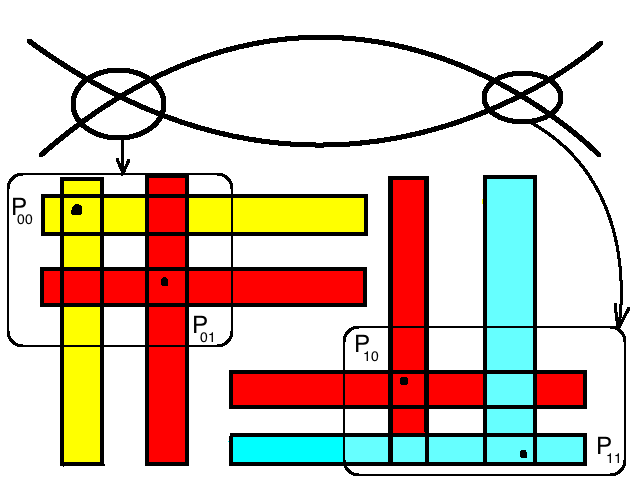
Figure 6: Isolating blocks for NHIL

To define centers of isolating blocks $P_{ij},\ i,j=\{0,1\}$ as on Fig. 6 we prove existence of four sets of functions:

$$\begin{aligned} h_{ii}(\eta,\xi,\varepsilon),\ w_{ii}(\eta,\xi,\varepsilon),\ \tau_{i}(\eta,\xi,\varepsilon),\quad i=0,1\qquad\text{and }\\ h_{ij}(\eta,\xi,\varepsilon),\ w_{ij}(\eta,\xi,\varepsilon),\ \tau_{ij}(\eta,\xi,\varepsilon),\quad i\neq j,\ i,j\in\{0,1\}.\end{aligned}$$ (26)

such that for all $(\xi,\eta)\in{\bf K}\times\mathbb{T}$ equations (41) and (44) hold. See Lemmas 3.4 and 3.5. We also have

$$w_{*}(\eta,\xi,\varepsilon)\equiv h_{*}(\eta,\xi,\varepsilon)-\frac{\eta^{2}}{2}.$$

In Lemma 3.3 we compute eigenvectors $v_{j}(x)$ and eigenvalues $\lambda_{j}(x),\ j=1,\dots,4$ of the rescaled linearization of the separatrix map (under new $(\eta,\xi,I,t)-$coordinate). Since $\mathcal{SM}_{\varepsilon}$ is symplectic, eigenvalues of its linearization $D\mathcal{SM}_{\varepsilon}$ at any point at come in pairs: one pair of eigenvalues $\lambda_{1,2}$ is close to one, the other pair is $\lambda_{3}\sim c\delta$ and $\lambda_{4}\sim(c\delta)^{-1}$. Note that there is no immediate dynamical implication from these eigenvectors as we do not claim existence of fixed points. However, these eigenvectors are used to construct a cone field in section 3.4.

Denote for $i,j\in\{0,1\}$

$$v_{4}^{ij}(\eta,\xi,\varepsilon)=v_{4}^{ij}(\eta,\xi,h_{ij}(\eta,\xi,\varepsilon),\tau_{ij}(\eta,\xi,\varepsilon)).$$ (27)

Fix small $\delta>0$, some $\kappa>0$ and define the following four sets:

$$\begin{aligned} \Pi^{\delta,\kappa}_{ij}:=\left\{(\eta,\xi,h,\tau):\text{there is }(\eta_{0},\xi_{0})\in{\bf K}\times\mathbb{T},\ |\delta_{3}|\leq\kappa_{1}\delta,|\delta_{4}|\leq\kappa_{2}\delta^{2}\ \right.\\ \text{ such that }\quad(\eta,\xi,h,\tau)=\qquad\qquad\qquad\qquad\qquad\qquad\qquad\qquad\\ \left.(\eta_{0},\xi_{0},h_{ij}(\eta_{0},\xi_{0},\varepsilon),\tau_{ij}(\eta_{0},\xi_{0},\varepsilon))+\delta_{3}L_{\varepsilon}v_{3}^{ij}(\eta_{0},\xi_{0},\varepsilon)+\delta_{4}L_{\varepsilon}v_{4}^{ij}(\eta_{0},\xi_{0},\varepsilon)\right\}.\end{aligned}$$ (28)

These sets $\Pi^{\delta,\kappa}_{ij},\ i,j\in\{0,1\}$ can be viewed as the union of parallelograms centered at $(\eta_{0},\xi_{0},h^{ij}_{\varepsilon}(\eta_{0},\xi_{0}),\tau^{ij}_{\varepsilon}(\eta_{0},\xi_{0}))$ with $(\eta_{0},\xi_{0})$ varying inside ${\bf K}\times\mathbb{T}$.

Consider the Hamiltonian $H_{\varepsilon}=H_{0}+\varepsilon P_{N}$, given by (3) and let $P$ be a polynomial such that the associated Melnikov function $M^{\pm}$, given by Lemma 2.11, satisfies (24).

Let $\Sigma=\{0,1\}^{\mathbb{Z}}$ be the space of infinite sequences on two symbols, $\omega=(\dots,\omega_{-1},\omega_{0},\omega_{1},\dots)\in\Sigma$, and $\sigma:\Sigma\to\Sigma$ be the shift, i.e. $\sigma\omega=\omega^{\prime}$, where $\omega^{\prime}_{i+1}=\omega_{i}$ for all $i\in\mathbb{Z}$. Let $\mathbb{A}_{0}:=\mathcal{D}_{0}\times\mathbb{T}\subset\mathbb{A}:=\mathbb{R}\times\mathbb{T}$ be a cylinder, $(\eta,\xi)\in\mathcal{D}_{0}\times\mathbb{T}$. We call a map

$$F:\mathbb{A}_{0}\times\Sigma\to\mathbb{A}\times\Sigma$$

a $C^{r}$ smooth skew-product map, if it is given by

$$F:(\eta,\xi,\omega)\longmapsto(\eta^{\prime},\xi^{\prime},\omega^{\prime})=(f_{\omega}(\eta,\xi),\sigma\omega),$$

where $f_{\omega}:\mathbb{A}_{0}\to\mathbb{A}$ is a family of $C^{r}$ smooth cylinder maps with $C^{r}$ dependence on $\omega$, i.e. the difference of $f_{\omega}-f_{\omega^{\prime}}$ goes to zero with respect to the $C^{r}$ norm if $\omega-\omega^{\prime}\to 0$. See also Appendix C for related definitions.

Theorem 3.1.

Fix small $\rho>0$. Suppose the trigonometric polynomial $P$ from (4) satisfies (24) for small $a>0$, then for $\kappa^{s}>0$, depending on $H_{0}$ and $H_{1}$ only, and any $\varepsilon>0$ small enough the associated separatrix map $\mathcal{SM}_{\varepsilon}$, given by (2.8), has a NHIL, denoted ${\bf\Lambda}_{\varepsilon}$, i.e.

$${\bf\Lambda}_{\varepsilon}\subset\cup_{ij\in\{0,1\}}\ \Pi^{\delta,\varepsilon}_{ij}.$$

Moreover, there is a map

$$C:\mathbb{A}_{0}\times\Sigma\to{\bf\Lambda}_{\varepsilon}$$

such that for each $(\eta,\xi,\omega)\in\mathcal{D}_{0}\times\mathbb{T}\times\Sigma$ we have

$$\mathcal{SM}_{\varepsilon}(C(\eta,\xi,\omega))=C(f_{\omega}(\eta,\xi),\sigma\omega).$$

In other words, for a $C^{r}$ smooth skew-product map $F$ the following diagram commutes:

$$\begin{array}[c]{ccc}\quad\ {\bf\Lambda}_{\varepsilon}&\quad\stackrel{{\scriptstyle\mathcal{SM}_{\varepsilon}}}{{\longrightarrow}}&\quad{\bf\Lambda}_{\varepsilon}\\ C\ \uparrow&&C\ \uparrow\\ \ \ \ \ |&&\ \ \ \ |\\ \mathbb{A}_{0}\times\Sigma&\quad\stackrel{{\scriptstyle F}}{{\longrightarrow}}&\ \ \mathbb{A}\times\Sigma.\end{array}$$ (33)

In addition, there exists $k\in\mathbb{N}$ such that

$$[\omega]_{k}:=(\omega_{-k},\cdots,\omega_{0},\cdots,\omega_{k})$$

is a truncation and exist functions $\tau_{[\omega]_{k}}(\eta,\xi)$, $I_{[\omega]_{k}}(\eta,\xi)$ such that the map $F(\cdot,\omega)$ has the following form

$$\begin{aligned} \eta^{+}&=&\eta-\varepsilon M^{+}_{\xi}(\eta^{+},\xi,\tau_{[\omega]_{k}}(\eta,\xi))+{\bf O}_{2},\\ \xi^{+}&=&\xi+\epsilon M_{\eta^{+}}^{+}(\eta^{+},\xi,\tau_{[\omega]_{k}}(\eta,\xi))-\dfrac{\eta^{+}}{\lambda}\log\left|\dfrac{\kappa^{s}\,I_{[\sigma\omega]_{k}}(\eta^{+},\xi^{+})}{\lambda}\right|+{\bf O}_{1}.\end{aligned}$$ (34)

Remark 3.2.

Smallness of $a$ is independent from the size the compact domain ${\bf K}\subset\mathbb{R}$, because $\xi$-dependent components of the Melnikov function average out (see the proof of Lemma 2.12).

Notice that in (34) there exists one invalid term $\epsilon M_{\eta^{+}}^{+}(\eta^{+},\xi,\tau_{[\omega]_{k}}(\eta,\xi))$ because it’s smaller than the reminder $\mathbf{O}_{1}$. We leave it in this position to match the system (18) better.

Actually, $\Big{\{}(\eta,\xi,I_{\omega}(\eta,\xi),t_{\omega}(\eta,\xi))\Big{|}(\eta,\xi)\in{\bf K}\times\mathbb{T},\omega\in\Sigma\Big{\}}$ is the coordinate of NHIL (see section 3.5). The Hölder continuity of $\omega$ benefits us with a finite truncation and we just need to consider $I_{\omega,k}$ and $t_{\omega,k}$ instead. The error caused by truncation can be much less than the $\mathbf{O}_{1}$ and $\mathbf{O}_{2}$ terms.

Proof.

The proof consists of following parts:

• Derive properties of the linearization $D\mathcal{SM}_{\varepsilon}$ near zeroes of the Melnikov potential $M^{+}_{\tau}-\eta M^{+}_{\xi}=0$ such as eigenvalues and eigenvectors (see Lemma 3.3).

• Find an approximately invariant cylinders for separatrix map $\mathcal{SM}_{\varepsilon}$: for $i,j\in\{0,1\}$ we have

  $$C_{ij}:{\mathcal{D}}_{0}\times\mathbb{T}\to{\mathcal{D}}\times\mathbb{T}\times\mathbb{R}\times\mathbb{T}$$

  $$C(r,\theta)=(\eta(r,\theta),\xi(r,\theta),\tau_{ij}(\eta,\xi,\varepsilon),w_{ij}(\eta,\xi,\varepsilon))$$

  so that

  $$\mathcal{SM}_{\varepsilon}(C_{01}({\mathcal{D}}_{0}\times\mathbb{T}))\approx C_{10}({\mathcal{D}}_{0}\times\mathbb{T})$$

  $$\mathcal{SM}_{\varepsilon}(C_{10}({\mathcal{D}}_{0}\times\mathbb{T}))\approx C_{01}({\mathcal{D}}_{0}\times\mathbb{T}).$$

  These cylinders play the role of centers of the isolating blocks containing the normally hyperbolic lamination (see points $P_{ij}$ on Fig. 6).

• Show that for proper $\kappa$ the $\kappa_{1}\delta\times\kappa_{2}\delta^{2}$-paralellogram neighborhoods of these cylinders $\Pi^{\delta,\kappa}_{ij}$, given by (28) satisfy conditions [C1-C5].

• Prove NHIL’s Hölder dependence of $\omega$ and the smoothness of every leaf, which leads to a skew product satisfiy (34).

∎

3.2 Properties of the linearization of $\mathcal{SM}_{\varepsilon}$

We star with the setting of Corollary 2.5. Actually, (18) is enough to achieve the existence of NHIL. But we should keep in mind the reminders $\mathbf{O}_{1}$ and $\mathbf{O}_{2}$ can be further evaluated due to (2.8). In the sequel we limit to the symbol $\sigma=+$, in that we consider the map to be undefined when $w<0$, and show that $\mathcal{SM}_{\epsilon}$ has an NHIL. With almost the same procedure we can get the NHIL for the case $\sigma=-$. The system (18) can be seen as two coupled subsystems, to see this more clearly, define

$$I=\frac{1}{\epsilon}(h-E(\eta)),$$

which also includes a rescaling. Note that

$$\epsilon I^{+}=h^{+}-E(\eta^{+})=h-\epsilon M^{+}_{\tau}-[E(\eta)+E^{\prime}(\eta)(\eta^{+}-\eta)]+{\bf O}_{2}\\ =\epsilon I-\epsilon\bigl{(}M^{+}_{\tau}(\eta,\xi,\tau)-E^{\prime}(\eta)M^{+}_{\xi}(\eta,\xi,\tau)\bigr{)}+{\bf O}_{2}$$

since $\eta^{+}-\eta=O(\epsilon)$. We will also omit the superscripts from $M^{+}$ and $\kappa^{+}$. Then

$$\eta^{+} =\eta {}-\epsilon M_{\xi}(\eta,\xi,\tau) {}+{\bf O}_{2}$$ (35)

$$\xi^{+} =\xi {}+\epsilon M_{\eta}(\eta,\xi,\tau) -\frac{\eta^{+}}{\lambda}\log\left(\frac{\epsilon\kappa I^{+}}{\lambda}\right) {}+{\bf O}_{1}$$

$$I^{+} =I {}-\bigl{(}M_{\tau}-E^{\prime}(\eta)M_{\xi})(\eta,\xi,\tau\bigr{)} {}+\frac{1}{\epsilon}{\bf O}_{2}$$

$$\tau^{+} =\tau +\frac{1}{\lambda}\log\left(\frac{\epsilon\kappa I^{+}}{\lambda}\right) \mod 2\pi +\;{\bf O}_{1}$$

We removed the absolute value from the $\log$ term and noting the map is undefined for $I^{+}<0$. As (8) is mechanical, $\omega=h^{+}-{\eta^{+2}}/{2}$.

Lemma 3.3.

Consider the separatrix map $\mathcal{SM}_{\varepsilon}$ for the generalized example of Arnold (3-4). Suppose the Melnikov potential $M(\eta,\xi,\tau)$ satisfies condition [M1]. Then for some positive $C,\nu$ and any sufficiently small $\delta$ such that $\varepsilon^{\varpi}\leq\delta$, $1\geq\varpi>1/4$ for any

$$x=(\eta,\xi,I,\tau)\in{\bf K}\times\mathbb{T}\times(-C\delta,C\delta)\times\mathbb{T}$$

the differential D$\mathcal{SM}_{\varepsilon}$ has eigenvalues

$$|\lambda_{i}-1|\leq C\varepsilon^{1/8}\log\varepsilon,\ i=1,2,\qquad|\lambda_{4}|<C\delta,\ |\lambda_{3}|>\frac{1}{2C\delta}.$$

For $|\eta|\geq\nu$ there are eigenvectors $e_{j}(x),\ j=1,2,3,4$, i.e.

$$\textup{D}\mathcal{SM}_{\varepsilon}(x)\,e_{j}(x)=\lambda_{j}(x)e_{j}(x).$$ (36)

such that

$$e_{3}(x)=\frac{(0,\eta,0,-1)}{\sqrt{1+\eta^{2}}}+\mathcal{O}(\delta)$$

$$e_{4}(x)=\frac{(0,\eta,\Delta M,-1)}{\sqrt{1+\eta^{2}+\Delta M^{2}}}+\mathcal{O}(\delta^{2})$$

$$e_{1,2}(x)=\frac{(0,-M_{\tau\tau}+\eta M_{\xi\tau},0,M_{\xi\tau}-\eta M_{\xi\xi})}{\sqrt{(-M_{\tau\tau}+\eta M_{\xi\tau})^{2}+(-M_{\xi\tau}+\eta M_{\xi\xi})^{2}}}+\mathcal{O}(\epsilon^{1/8}\log\epsilon)$$

with $\Delta M=M_{\tau\tau}-2\eta M_{\tau\xi}+\eta^{2}M_{\xi\xi}$.

In particular, for each $(\eta,\xi)\in{\bf K}\times\mathbb{T}$ angles between $e_{i}(x)$ and $e_{j}(x)$ with $i\neq j$ and $\{i,j\}\neq\{1,2\}$ is uniformly away from zero. Moreover, for each $x$ such that $\delta$ satisfies the above conditions the vector $\textup{D}\mathcal{SM}_{\varepsilon}(x)e_{4}$ in absolute value is bounded by $C\delta$.

Proof.

Denote $w=\varepsilon\delta/\lambda$. The differential of the separatrix map D$\mathcal{SM}_{\varepsilon}^{+}$ for the Arnold’s example (18) is given by:

$$\begin{pmatrix}\frac{\partial\eta^{+}}{\partial\eta}&\frac{\partial\eta^{+}}{\partial\xi}&0&\frac{\partial\eta^{+}}{\partial\tau}\\ -\frac{1}{\lambda}\log\frac{\epsilon I^{+}}{\lambda}\frac{\partial\eta^{+}}{\partial\eta}-\frac{\eta^{+}}{\lambda I^{+}}\frac{\partial\Delta}{\partial\eta}&1-\frac{\eta^{+}}{\lambda I^{+}}\frac{\partial\Delta}{\partial\xi}-2\pi l\frac{\partial\eta^{+}}{\partial\xi}&-\frac{\eta^{+}}{\lambda I^{+}}&-\frac{\eta^{+}}{\lambda I^{+}}\frac{\partial\Delta}{\partial\tau}-2\pi l\frac{\partial\eta^{+}}{\partial\tau}\\ \frac{\partial\Delta}{\partial\eta}&\frac{\partial\Delta}{\partial\xi}&1&\frac{\partial\Delta}{\partial\tau}\\ \frac{1}{\lambda I^{+}}\frac{\partial\Delta}{\partial\eta}&\frac{1}{\lambda I^{+}}\frac{\partial\Delta}{\partial\xi}&\frac{1}{\lambda I^{+}}&1+\frac{1}{\lambda I^{+}}\frac{\partial\Delta}{\partial\tau}\\ \end{pmatrix}+\begin{pmatrix}\mathbf{O}_{2}\\ \mathbf{O}_{1}\\ \mathbf{O}_{2}/\epsilon\\ \mathbf{O}_{1}\end{pmatrix},$$

which can be translated into

$$\left(\begin{array}[]{cccc}1-\varepsilon M_{\xi\eta}&-\varepsilon M_{\xi\xi}&0&-\varepsilon M_{\xi\tau}\\ \vskip 6.0pt plus 2.0pt minus 2.0pt\cr-\eta^{+}\frac{-M_{\tau\eta}+M_{\xi}+\eta M_{\xi\eta}}{\lambda I^{+}}-(1-\varepsilon M_{\xi\eta})\log\left|{\varepsilon I^{+}}\right|&1-\frac{\eta^{+}\,\gamma}{\lambda I^{+}}+\varepsilon M_{\xi\xi}\log|{\varepsilon I^{+}}|&\frac{-\eta^{+}}{\lambda I^{+}}&\frac{-\eta^{+}\,\alpha}{\lambda I^{+}}+\varepsilon M_{\xi\tau}\log|{\varepsilon I^{+}}|\\ \vskip 6.0pt plus 2.0pt minus 2.0pt\cr-M_{\tau\eta}+M_{\xi}+\eta M_{\xi\eta}&\gamma&1&\alpha\\ \vskip 6.0pt plus 2.0pt minus 2.0pt\cr\frac{-M_{\tau\eta}+M_{\xi}+\eta M_{\xi\eta}}{\lambda I^{+}}&{\frac{\gamma}{\lambda I^{+}}}&{\frac{1}{\lambda I^{+}}}&1+{\frac{\alpha}{\lambda I^{+}}}\end{array}\right),$$

where:

$$\Delta=-M_{\tau}+\eta M_{\xi},$$

$$\gamma=-M_{\xi\tau}+\eta M_{\xi\xi},$$

$$\alpha=-M_{\tau\tau}+\eta M_{\xi\tau},$$

$$\zeta=-M_{\tau\eta}+M_{\xi}+\eta M_{\xi\eta},$$

$$\beta=\frac{1}{\lambda I^{+}},$$

$$l\in\mathbb{Z}\;\text{such that}\;l=[\frac{1}{2\pi\lambda}\log\frac{\kappa\epsilon}{\lambda}]$$

and the error of entries in the first and third rows is $\mathcal{O}(\varepsilon^{5/4}\log^{2}\varepsilon)$, $\mathcal{O}(\varepsilon^{1/4}\log^{2}\varepsilon)$ and the error of entries in the second and forth rows is $\mathcal{O}(\varepsilon^{7/8}\log^{2}\varepsilon)$. Notice that the $\kappa$ and $\lambda$ are just contants in the original separatrix map (8), so we can remove them from the matrix.

As the separatrix map is symplectic, the determinant of this matrix should be one (although we take a new coordinate). So we can get a couple of eigenvalues close to 1

$$\lambda_{1,2}(x)=1\pm\mathcal{\mathcal{missing}}O(\varepsilon^{1/8}\log\varepsilon).$$

This point can be verified from a simple calculation:

$$det(D\mathcal{SM}_{\epsilon}^{+}-\lambda Id)=(1-\lambda)^{4}-(1-\lambda)^{2}\lambda\frac{\alpha-\eta\gamma}{\delta}+\mathcal{O}(\epsilon^{1/4}\log^{2}\epsilon)=0.$$

Neglecting error terms of order $\mathcal{O}(\varepsilon^{1/4}\log^{2}\varepsilon)$, we get

$$\text{trace}(\text{D}\mathcal{SM}_{\varepsilon}^{+})=4+\frac{\alpha-\eta\gamma}{\delta}.$$ (37)

Due to [M1], for each $(\eta,\xi)\in{\bf K}\times\mathbb{T}$ we have

$$\alpha-\eta\gamma=\Delta M=M_{\tau\tau}-2\eta M_{\tau\xi}+\eta^{2}M_{\xi\xi}\neq 0$$

uniformly hold, then for small enough $\delta$, this trace should be $\mathcal{O}(1/\delta)$. So there should existsthe other couple of eigenvalues

$$\lambda_{3}(x)\sim\mathcal{O}(1/\delta),\quad\lambda_{4}(x)\sim\mathcal{O}(\delta)$$

because the determinant equals one.

Now we compute approximation of the eigenvectors:

$$D\mathcal{SM}_{\varepsilon}(x)e_{j}(x)=\lambda_{j}(x)e_{j}(x),\quad j=1,2,3,4,$$

so we can estimate the eigenvalues

$$\lambda_{1,2} =1+\mathcal{O}(\epsilon^{1/8}\log\epsilon),$$ (38)

$$\lambda_{3} =\frac{2+\alpha\beta-\eta^{+}\beta\gamma+sgn(\alpha)\sqrt{(2+\alpha\beta-\eta^{+}\beta\gamma)^{2}-4}}{2}+\mathcal{O}(\epsilon/\delta),$$

$$\lambda_{4} =\frac{2+\alpha\beta-\eta^{+}\beta\gamma-sgn(\alpha)\sqrt{(2+\alpha\beta-\eta^{+}\beta\gamma)^{2}-4}}{2}+\mathcal{O}(\epsilon\delta),$$

and corresponding eigenvectors by

$$e_{1,2} =(0,\frac{\alpha}{\sqrt{\alpha^{2}+\gamma^{2}}},0,-\frac{\gamma}{\sqrt{\alpha^{2}+\gamma^{2}}})^{t}+\mathcal{O}(\epsilon^{1/8}\log\epsilon),$$ (39)

$$e_{3} =\frac{|\lambda_{3}-1|\cdot|\beta|}{\sqrt{\lambda_{3}^{2}(1+\eta^{+2})\beta^{2}+(\lambda_{3}-1)^{2}}}(0,\frac{\eta^{+}\lambda_{3}}{1-\lambda_{3}},\frac{1}{\beta},\frac{\lambda_{3}}{\lambda_{3}-1})^{t}+\mathcal{O}(\delta),$$

$$\approx\frac{1}{\sqrt{1+\eta^{2}}}(0,\eta,0-1)+\mathcal{O}(\delta),$$

$$e_{4} =\frac{1}{\sqrt{\lambda_{4}^{2}\beta^{2}(1+\eta^{+2})+(\lambda_{4}-1)^{2}}}(0,-\lambda_{4}\beta\eta^{+},\lambda_{4}-1,\lambda_{4}\beta)^{t}+\mathcal{O}(\delta^{2}),$$

$$\approx\frac{1}{\sqrt{1+\eta^{2}+(\alpha-\eta\gamma)^{2}}}(0,\eta,\alpha-\eta\gamma,-1)+\mathcal{O}(\delta^{2})$$

with $\beta\sim\mathcal{O}(1/\delta)$. [M1] ensures the angles between different eigenvectors are uniformly away from zero. Change $\alpha$, $\gamma$ back into the notation depending on $M$ we proved the Lemma.

∎

3.3 Calculation of centers of isolating blocks

In this section we calculate the set of functions $w$’s and $h$’s from (26). Recall that the sepatatrix map can be written in the new coordinate

$$\mathcal{SM}_{\varepsilon}(\eta,\xi,I,\tau)=(\eta^{+},\xi^{+},I^{+},\tau^{+})$$

with $w=\epsilon I+\epsilon\Delta(\eta,\xi,\tau)+\mathbf{O}_{2}$. So we just need to get weak invariant functions

$$\begin{aligned} I_{ii}(\eta,\xi,\varepsilon),\ \tau_{ii}(\eta,\xi,\varepsilon),\quad i=0,1\qquad\text{and }\\ I_{ij}(\eta,\xi,\varepsilon),\ \tau_{ij}(\eta,\xi,\varepsilon),\quad i\neq j,\ i,j\in\{0,1\}\end{aligned}$$ (40)

which satisfy the following Lemma.

Lemma 3.4.

Suppose condition (24) holds for a sufficiently small $a>0$. Fix $1\geq\varpi>1/4>\rho>0$. Then for a sufficiently small $\varepsilon>0$ and $\delta\in(\varepsilon^{\varpi},\varepsilon^{\rho})$ there are functions $\tau_{ii}$ and $I_{ii},\ i=0,1$ such that $I_{ii}=\mathcal{O}(\delta)$ and these functions satisfy

$$\begin{aligned} \eta^{+}&=\eta-\varepsilon M^{+}_{\xi}(\eta,\xi,\tau_{ii}(\xi,\eta,\varepsilon))\\ \xi^{+}&=\xi+\varepsilon M^{+}_{\eta^{+}}(\eta,\xi,\tau_{ii}(\xi,\eta,\varepsilon))-\dfrac{\eta^{+}}{\lambda}\log\left|\dfrac{\kappa^{+}\epsilon I_{ii}(\xi^{+},\eta^{+},\varepsilon)}{\lambda}\right|\;\text{mod}\;2\pi\\ \left|\ \tau_{ii}\right.&\left.(\eta,\xi,\varepsilon)+2n\pi+\frac{1}{\lambda}\ \log\left|\dfrac{\kappa^{+}\epsilon I_{ii}(\xi^{+},\eta^{+},\varepsilon)}{\lambda}\right|-\tau_{ii}(\eta^{+},\xi^{+},\varepsilon)\right|\leq\mathcal{O}(a\,\delta^{2})\\ \left|I_{ii}\right.&\left.(\eta,\xi,\varepsilon)+\Delta(\eta,\xi,\tau_{ii}(\eta,\xi,\varepsilon))-I_{ii}(\eta^{+},\xi^{+},\varepsilon)\right|\leq\mathcal{O}(\delta^{2}),\end{aligned}$$ (41)

where $I_{ii}(\eta,\xi,\varepsilon)>0$ for all $(\eta,\xi)\in{\bf K}\times\mathbb{T}$.

Moreover, these solutions satisfy

$$I_{ii}(\eta,\xi,\varepsilon) = \delta+a\delta\bar{I}_{ii}(\eta,\xi,a)$$ (42)

$$\tau_{ii}(\eta,\xi,\varepsilon) = {i\pi}+a\tau_{i}^{1}(\eta,\xi,a)+a\delta\,\tau_{ii}^{2}(\eta,\xi,a)$$

for some smooth functions $\bar{I}_{ii},\ \tau_{i}^{1},\ \tau_{ii}^{2}$ with $i\pi+a\tau_{i}^{1}$ solving the first implicit equation in [M1].

Notice that this lemma says that neglecting the error terms in the separatrix map $\mathcal{SM}_{\varepsilon}$ from Corollary 2.5 has two weak invariant cylinders

$$\Lambda_{ii}=\{(\eta,\xi,h_{ii}(\eta,\xi),\tau_{ii}(\eta,\xi)):\ (\eta,\xi)\in{\bf K}\times\mathbb{T}\}$$

with $\omega_{ii}=I_{ii}(\eta,\xi,\epsilon)+\Delta(\eta,\xi,\tau_{ii}(\eta,\xi,\epsilon))$ and $h_{ii}=\epsilon I_{ii}+\eta^{2}/2$. Denote by $\Lambda_{ii}^{*}$ the invariant cylinder obtained by extending $h_{ii}$ and $\tau_{ii}$ for an $O(\varepsilon)$-neighbourhood of $\bf K$. Then up to error terms $\mathcal{SM}_{\varepsilon}(\Lambda_{ii})\subset\Lambda^{*}_{ii}.$

Proof.

Start by proving existence of $w_{ii},\,\tau_{ii}$’s solving functional equations (41) for $i=0,1$.

• By M1 we have

  $$M^{+}_{\tau}(\eta,\xi,\tau_{i}(\eta,\xi))-\eta M^{+}_{\xi}(\eta,\xi,\tau_{i}(\eta,\xi))=0.$$

  Actually we can take $\tau_{i}(\eta,\xi)={i\pi}+a\tau_{i}^{1}(\eta,\xi,a)$ where $a$ is sufficiently small. This can be derived from the $\mathcal{O}(a)$ estimate. We formally solve the $\tau_{i}^{1}(\eta,\xi,a)$ by

  $$\tau_{i}^{1}(\eta,\xi,a)=\frac{\partial_{t}\overline{M}(\eta,\xi,i\pi)-\eta\partial_{\xi}\overline{M}(\eta,\xi,i\pi)}{2\pi\cos i\pi}+\mathcal{O}(a).$$

• Take the formal solution (42) into the separatrix map. It should satisfies

  $$\eta^{+} =\eta-a\epsilon\partial_{\xi}\overline{M}^{s}(\eta,\xi,\tau_{ii}(\eta,\xi,a))+\mathbf{O}_{2},$$ (43)

  $$\xi^{+} =\xi+2\pi\{n\eta\}-\frac{\eta}{\lambda}\log(1+a{\bar{I}_{ii}(\eta^{+},\xi^{+})})+\mathbf{O}_{1},$$

  $$a\delta\bar{I}_{ii}(\eta^{+},\xi^{+}) =a\delta\bar{I}_{ii}(\eta,\xi)-\Big{\{}\Delta(\eta,\xi,i\pi+a\tau_{i}^{1})+[\partial_{tt}M^{s}(i\pi+a\tau_{i}^{1})$$

  $$-a\eta\partial_{\xi t}\overline{M}(i\pi+a\tau_{i}^{1})\big{]}a\delta\tau_{ii}^{2}\Big{\}}+\mathcal{O}(a^{2}\delta^{2}),$$

  $$a\tau_{i}^{1}(\eta^{+},\xi^{+}) =a\tau_{i}^{1}(\eta,\xi)+\frac{1}{\lambda}\ln(1+{a\bar{I}_{ii}(\eta^{+},\xi^{+})})+\mathcal{O}(a\delta),$$

  where $\delta=\frac{\lambda}{\kappa\epsilon}\exp(2n\lambda\pi)$. Within the third equation,

  $$\Delta(\eta,\xi,i\pi+a\tau_{i}^{1})=0$$

  due to the first item, and

  $$\partial_{tt}M^{s}(i\pi+a\tau_{i}^{1})-a\eta\partial_{\xi t}\overline{M}(i\pi+a\tau_{i}^{1})\neq 0$$

  as $a$ sufficiently small. So we can update the third equation into

  $$\bar{I}_{ii}(\eta^{+},\xi^{+})=\bar{I}_{ii}(\eta,\xi)+\alpha(\eta,\xi,i\pi+a\tau_{i}^{1})\tau_{ii}^{2}+\mathcal{O}(a\delta)$$

  with $\alpha$ defined in previous section. Since $\eta$ belongs to a compact region $\bf K$, $a$ can be chosen sufficiently small and

  $$\bar{I}_{ii}(\eta^{+},\xi^{+}) =\bar{I}_{ii}(\eta,\xi^{+})+\mathcal{O}(a\epsilon)$$

  $$=\bar{I}_{ii}(\eta,\xi+2\pi\{n\eta\}-\frac{\eta}{\lambda}\ln(1+a{\bar{I}_{ii}(\eta^{+},\xi^{+})}))+\mathbf{O}_{1}$$

  $$=\bar{I}_{ii}(\eta,\xi+2\pi\{n\eta\}-\frac{\eta}{\lambda}\ln(1+a{\bar{I}_{ii}(\eta,\xi+2\pi\{n\eta\})}))+\mathcal{O}(a^{2}),$$

  so we solve the fourth equation of (43) and get

  $$\bar{I}_{ii}(\eta,\sigma(\eta,\xi))=\lambda[\tau_{i}^{1}(\eta,\sigma(\eta,\xi))-\tau_{i}^{1}(\eta,\xi)]+\mathcal{O}(a)$$

  where $\sigma(\eta,\xi)=\xi+2\pi\{n\eta\}$. Take this equation back into the third equation of (43) and get

  $$\tau_{ii}^{2}(\eta,\xi)=\frac{\bar{I}_{ii}(\eta,\sigma(\eta,\xi))-\bar{I}_{ii}(\eta,\xi)}{\alpha(i\pi+a\tau_{i}^{1})}+\mathcal{O}(a\delta).$$

∎

Lemma 3.5.

Suppose condition (24) holds for a sufficiently small $a>0$. Fix $1\geq\varpi>1/4>\rho>0$. Then for a sufficiently small $\varepsilon>0$ and $\delta\in(\varepsilon^{\varpi},\varepsilon^{\rho})$ there are functions $\tau_{ij}$ and $I_{ij},\ \{i,j\}=\{0,1\}$ such that $I_{ij}=\mathcal{O}(\delta)$ and these functions satisfy

$$\begin{aligned} \eta^{+}&=\eta-\varepsilon M^{+}_{\xi}(\eta,\xi,\tau_{ij}(\xi,\eta,\varepsilon))\\ \xi^{+}&=\xi+\varepsilon M^{+}_{\eta^{+}}(\eta,\xi,\tau_{ij}(\xi,\eta,\varepsilon))-\dfrac{\eta^{+}}{\lambda}\log\left|\dfrac{\kappa^{+}w_{ji}(\xi^{+},\eta^{+},\varepsilon)}{\lambda}\right|\\ \left|\ \tau_{ij}\right.&\left.(\eta,\xi,\varepsilon)+2n\pi+\frac{1}{\lambda}\ \log\left|\dfrac{\kappa^{+}w_{ij}(\xi^{+},\eta^{+},\varepsilon)}{\lambda}\right|-\tau_{ji}(\eta^{+},\xi^{+},\varepsilon)\right|\leq\mathcal{O}(a\,\delta^{2})\\ \left|I_{ij}\right.&\left.(\eta,\xi,\varepsilon)-\left[M^{+}_{\tau}(\eta,\xi,\tau_{ij}(\eta,\xi,\varepsilon))-\eta M^{+}_{\xi}(\eta,\xi,\tau_{ij}(\eta,\xi,\varepsilon))\right]\right.\\ &\left.\qquad\qquad\qquad\qquad\qquad\qquad-I_{ji}(\eta^{+},\xi^{+},\varepsilon)\right|\leq\mathcal{O}(\delta^{2}),\end{aligned}$$ (44)

where $I_{ij}(\eta,\xi,\varepsilon)>0$ for all $(\eta,\xi)\in{\bf K}\times\mathbb{T}$.

Moreover, these solutions satisfy

$$I_{ij}(\eta,\xi,\varepsilon)=\delta e^{-\lambda\pi}(1+a\bar{I}_{ij}(\eta,\xi,a))$$ (45)

$$\tau_{ij}(\eta,\xi,\varepsilon)={i\pi}+a\tau_{i}^{1}(\eta,\xi,a)+a\delta\,\tau_{ij}^{2}(\eta,\xi,a)$$

for some smooth functions $\bar{I}_{ij},\ \tau_{i}^{1},\ \tau_{ij}^{2}$ with $i\pi+a\tau_{i}^{1}$ solving the first implicit equation in [M1].

Neglecting the error terms in the square of separatrix map $\mathcal{SM}_{\varepsilon}^{2}$ from Corollary 2.5 we get two weak invariant cylinders

$$\Lambda_{ij}=\{(\eta,\xi,h_{ij}(\eta,\xi),\tau_{ij}(\eta,\xi)):\ (\eta,\xi)\in{\bf K}\times\mathbb{T}\}$$

with $\omega_{ij}=I_{ij}(\eta,\xi,\epsilon)+\Delta(\eta,\xi,\tau_{ij}(\eta,\xi,\epsilon))$ and $h_{ij}=\epsilon I_{ij}+\eta^{2}/2$. Denote by $\Lambda_{ij}^{*}$ the invariant cylinder obtained by extending $h_{ij}$ and $\tau_{ij}$ for an $O(\varepsilon)$-neighbourhood of $\bf K$. Then up to error terms $\mathcal{SM}_{\varepsilon}(\Lambda_{ij})\subset\Lambda^{*}_{ji}.$

Proof.

We use almost the same procedure as previous Lemma. Start by proving existence of $w_{ij},\ \tau_{ij}$’s solving functional equations (41) for $\{i,j\}=\{0,1\}$.

• Recall that we have already solved the $\tau_{i}^{1}(\eta,\xi)$ by

  $$\tau_{i}^{1}(\eta,\xi,a)=\frac{\partial_{t}\overline{M}(\eta,\xi,i\pi)-\eta\partial_{\xi}\overline{M}(\eta,\xi,i\pi)}{2\pi\cos i\pi}+\mathcal{O}(a),$$

  which satisifes

  $$M^{+}_{\tau}(\eta,\xi,i\pi+a\tau_{i}^{1}(\eta,\xi))-\eta M^{+}_{\xi}(\eta,\xi,i\pi+a\tau_{i}^{1}(\eta,\xi))=0.$$

• Take the formal solution (45) into the separatrix map, which should satisfies

  $$\left\{\begin{aligned} \eta^{+}&=\eta-a\epsilon\partial_{\xi}\overline{M}^{s}(\eta,\xi,\tau_{01}(\eta,\xi,a))+\mathbf{O}_{2},\\ \xi^{+}&=\xi+2\pi\{(n-\frac{1}{2})\eta\}-\frac{\eta}{\lambda}\ln(1+a{\bar{I}_{10}(\eta^{+},\xi^{+})})+\mathbf{O}_{1},\\ \bar{I}_{10}(\eta^{+},\xi^{+},a)&=\bar{I}_{01}(\eta,\xi,a)+\alpha(\eta,\xi,i\pi+a\tau_{0}^{1}(\eta,\xi,a))\tau_{01}^{2}+\mathcal{O}(a\delta)\\ a\tau_{1}^{1}(\eta^{+},\xi^{+},a)&=a\tau_{0}^{1}(\eta,\xi)+\frac{1}{\lambda}\ln(1+{a\bar{I}_{10}(\eta^{+},\xi^{+},a)})+\mathcal{O}(a\delta),\end{aligned}\right.$$ (46)

  and

  $$\left\{\begin{aligned} \eta^{+}&=\eta-a\epsilon\partial_{\xi}\overline{M}^{s}(\eta,\xi,\tau_{10}(\eta,\xi,a))+\mathbf{O}_{2},\\ \xi^{+}&=\xi+2\pi\{(n-\frac{1}{2})\eta\}-\frac{\eta}{\lambda}\ln(1+a{\bar{I}_{01}(\eta^{+},\xi^{+})})+\mathbf{O}_{1},\\ \bar{I}_{01}(\eta^{+},\xi^{+},a)&=\bar{I}_{10}(\eta,\xi,0)+\alpha(\eta,\xi,i\pi+a\tau_{1}^{1})\tau_{10}^{2}+\mathcal{O}(a\delta)\\ a\tau_{0}^{1}(\eta^{+},\xi^{+},a)&=a\tau_{1}^{1}(\eta,\xi)+\frac{1}{\lambda}\ln(1+{a\bar{I}_{01}(\eta^{+},\xi^{+},a)})+\mathcal{O}(a\delta).\end{aligned}\right.$$ (47)

  Recall that

  $$\alpha(\eta,\xi,i\pi+a\tau_{i}^{1})\neq 0,\quad i=0,1,$$

  uniformly hold for sufficient small $a$ and

  $$\xi^{+}=\xi+2\pi\{(n-\frac{1}{2})\eta\}+\mathcal{O}(a)$$

  because $\eta$ belongs to a compact region $\bf K$ and $a$ can be chosen sufficiently small. So we can solve the solution by

  $$\left\{\begin{aligned} \bar{I}_{10}(\eta,\sigma)&=\lambda(\tau_{1}^{1}(\eta,\sigma)-\tau_{0}^{1}(\eta,\xi))+\mathcal{O}(a),\\ \bar{I}_{01}(\eta,\sigma)&=\lambda(\tau_{0}^{1}(\eta,\sigma)-\tau_{1}^{1}(\eta,\xi))+\mathcal{O}(a),\\ \end{aligned}\right.$$ (48)

  and

  $$\left\{\begin{aligned} \tau_{01}^{2}(\eta,\xi)&=\frac{\bar{I}_{10}(\eta,\sigma)-\bar{I}_{01}(\eta,\xi)}{\alpha(\eta,\xi,i\pi+a\tau_{ii}^{1})}+\mathcal{O}(a\delta),\\ \tau_{10}^{2}(\eta,\xi)&=\frac{\bar{I}_{01}(\eta,\sigma)-\bar{I}_{10}(\eta,\xi)}{\alpha(\eta,\xi,i\pi+a\tau_{ii}^{1})}+\mathcal{O}(a\delta),\\ \end{aligned}\right.$$ (49)

  where $\sigma(\eta,\xi)=\xi+2\pi\{(n-\frac{1}{2})\eta\}$ and $\delta=\frac{\lambda}{\kappa\epsilon}\exp(2n\lambda\pi)$.

∎

3.4 Verification of isolating block conditions [C1-C5]

In this section we isolating blocks $\Pi^{u,s,\kappa}_{ij}=\Pi_{ij},i,j=\{0,1\}$ and verify C1-C3 for them. Then we define cone field over each point in isolating blocks and verify C4-C5. Recall that In Lemma 3.3 we compute eigenvectors $e_{j}(x)$ and eigenvalues $\lambda_{j}(x),\ j=1,\dots,4$ of the $\text{D}\mathcal{SM}_{\varepsilon}(x)$.

Since the map $\mathcal{SM}_{\varepsilon}$ is symplectic, eigenvalues come in pairs: one pair of eigenvalues $\lambda_{1,2}$ is close to one, the other pair is $\lambda_{3}\sim c\delta$ and $\lambda_{4}\sim(c\delta)^{-1}$. Besides, from Lemma 3.4 and Lemma 3.5 we get the eigenvectors based on the centers by

$$v_{s}^{ij}(\eta,\xi,\varepsilon)=v_{s}^{ij}(\eta,\xi,I_{ij}(\eta,\xi,\varepsilon),\tau_{ij}(\eta,\xi,\varepsilon)),\quad s=3,4.$$

For small $\delta>0$ and properly large $\kappa>0$ we define the following four sets:

$$\begin{aligned} \Pi^{s,\kappa}_{ij}:=\left\{(\eta,\xi,I,\tau):\text{there is }(\eta_{0},\xi_{0})\in{\bf K}\times\mathbb{T},\qquad\qquad\qquad\qquad\qquad\qquad\qquad\right.\\ |c|\leq\kappa_{1}\delta^{2},|d|\leq\kappa_{2}\delta\ \text{ such that }\qquad\qquad\qquad\qquad\qquad\qquad\qquad\qquad\\ \left.(\eta,\xi,I,\tau)=(\eta_{0},\xi_{0},I_{ij}(\eta_{0},\xi_{0},\varepsilon),\tau_{ij}(\eta_{0},\xi_{0},\varepsilon))+cv_{3}^{ij}(\eta_{0},\xi_{0},\varepsilon)+dv_{4}^{ij}(\eta_{0},\xi_{0},\varepsilon)\right\}.\end{aligned}$$ (50)

We drop $\varepsilon$-dependence for brievity. These sets $\Pi^{s,\kappa}_{ij},\ i,j\in\{0,1\}$ can be viewed as the union of parallelograms centered at $(\eta_{0},\xi_{0},I^{ij}_{\varepsilon}(\eta_{0},\xi_{0}),\tau^{ij}_{\varepsilon}(\eta_{0},\xi_{0}))$ with $(\eta_{0},\xi_{0})$ varying inside ${\bf K}\times\mathbb{T}$.

By Lemma 3.3 we derive that these eigenvectors of $D\mathcal{SM}_{\varepsilon}$ have the following form:

$$e_{3}(x)=\frac{(0,\eta,0,-1)}{\sqrt{1+\eta^{2}}}+\mathcal{O}(\delta)$$

$$e_{4}(x)=\frac{(0,\eta,\Delta M,-1)}{\sqrt{1+\eta^{2}+\Delta M^{2}}}+\mathcal{O}(\delta^{2})$$

$$e_{1,2}(x)=\frac{(0,-M_{\tau\tau}+\eta M_{\xi\tau},0,M_{\xi\tau}-\eta M_{\xi\xi})}{\sqrt{(-M_{\tau\tau}+\eta M_{\xi\tau})^{2}+(-M_{\xi\tau}+\eta M_{\xi\xi})^{2}}}+\mathcal{O}(\epsilon^{1/8}\log\epsilon).$$

Define

$$\psi:=\min\{\measuredangle(v_{3}(x),v_{4}(x)):\ x\in\Pi_{ij},\ i,j\in\{0,1\}\}.$$

Lemma 3.6.

If condition [M1] holds, then $\psi>0$ uniformly holds.

Proof.

By definition $v_{3}(x)\parallel\approx(0,\eta,0,-1)$ and $v_{4}(x)\parallel\approx(0,\eta,\alpha-\eta\gamma,-1)$. By condition [M1] we have

$$\Delta M=\alpha-\eta\gamma\neq 0$$

uniformly for $(\eta,\xi)\in\mathbf{K}\times\mathbb{T}$. ∎

Figure 7: Isolating Block

For any point in the isolating block $\Pi_{ij}^{s,\kappa}$, we can define a local transformation by:

$$\Phi_{ij}:(\eta,\xi,I,\tau)\rightarrow(\eta_{0},\xi_{0},c,d),$$

where $c$ and $d$ are the projections of $(\eta-\eta_{0},\xi-\xi_{0},I-I_{ij}(\eta_{0},\xi_{0}),\tau-\tau_{ij}(\eta_{0},\xi_{0}))$ to $e_{3}$ and $e_{4}$ with $(\eta_{0},\xi_{0})$ the corrsponding point in the center. Under this new coordinate, we have

$$\mathfrak{SM}_{\epsilon}:=\Phi_{ji}\circ\mathcal{SM}_{\epsilon}\circ\Phi_{ij}^{-1}$$

defined on the new straight grids

$$\mathfrak{N}_{ij}^{s,\kappa}=\Phi_{ij}(\Pi_{ij}^{s,\kappa}).$$

Then we can prove the following stronger conditions:

Lemma 3.7.

$$\Big{|}\pi_{4}\circ\mathfrak{SM}_{\epsilon}\mathfrak{N}_{ij}^{s,\kappa}\Big{|}\leq\mathcal{O}(\delta^{2}),$$ (51)

$$\Big{|}\pi_{3}\circ\mathfrak{SM}_{\epsilon}\mathfrak{N}_{ij}^{s,\kappa}\Big{|}\geq\mathcal{O}(\delta)$$ (52)

and

$$\mathfrak{SM}_{\epsilon}\partial^{u}\mathfrak{N}_{ij}^{s,\kappa}\simeq\partial^{u}\mathfrak{N}_{ij}^{s,\kappa},$$ (53)

for any $(\eta,\xi)\in\mathbf{K}\times\mathbb{T}$. Here $\partial^{u}$ means the boundary of the 3-rd component and $\simeq$ means homotopic equivalence.

Recall that C3 is actually ensured by the weak invariance of centers in aforementioned section. So in the following we just need to prove C1 and C2, which can be derived from this Lemma.

Proof.

We remove the $\epsilon$ dependence for convenience. $\forall({\eta},\xi,I,\tau)\in\Pi_{ij}^{s,\kappa}$, which corresponds to a unique point $(\eta_{0},\xi_{0},c,d)\in\mathfrak{N}_{ij}^{s,\kappa}$, we get

$$\mathfrak{SM}(\eta_{0},\xi_{0},c,d)- (\eta_{0}^{+},\xi^{+}_{0},0,0)=\Phi_{ji}[\mathcal{SM}(\eta,\xi,I,\tau)-(\eta_{0}^{+},\xi_{0}^{+},I_{ji}(\eta_{0}^{+},\xi_{0}^{+}),\tau_{ji}(\eta_{0}^{+},\xi_{0}^{+}))]$$ (54)

$$=\Phi_{ji}\int_{0}^{1}D\mathcal{SM}(s\eta+(1-s)\eta_{0},s\xi+(1-s)\xi_{0},sI+$$

$$\quad\quad(1-s)I_{ij}(\eta_{0},\xi_{0}),s\tau+(1-s)\tau_{ij}(\eta_{0},\xi_{0}))\cdot(cv_{3}^{ij}+dv_{4}^{ij})ds$$

$$=\Phi_{ji}\Big{[}D\mathcal{SM}(\eta_{0},\xi_{0},I_{ij}(\eta_{0},\xi_{0}),\tau_{ij}(\eta_{0},\xi_{0}))\cdot(cv_{3}^{ij}+dv_{4}^{ij})+$$

$$\quad\quad\int_{0}^{1}\Upsilon(s)(cv_{3}^{ij}+dv_{4}^{ij})ds\Big{]}$$

$$=\Phi_{ji}\Big{[}c\lambda_{3}v_{3}^{ij}+d\lambda_{4}v_{4}^{ij}+\int_{0}^{1}(\Upsilon^{\prime}+\mathcal{O}(\kappa_{2},\delta))(cv_{3}^{ij}+dv_{4}^{ij})ds\Big{]},$$

where $\Upsilon(s)=D\mathcal{SM}\Big{|}_{0}^{s}$ is a variational matrix with $s\in(0,1)$. Formally it equals to

$$\begin{pmatrix}0&0&0&0\\ Osc(-\frac{1}{\lambda}\ln I^{+}-\eta^{+}\beta\zeta)&Osc(-\eta^{+}\beta\gamma)&Osc(-\eta^{+}\beta)&Osc(-\eta^{+}\beta\alpha)\\ Osc(\zeta)&Osc(\gamma)&0&Osc(\alpha)\\ Osc(\zeta\beta)&Osc(\beta\gamma)&Osc(\beta)&Osc(\beta\alpha)\\ \end{pmatrix}+\delta\mathbf{O}_{1},$$

where the ‘Osc’ means the variation between $0$ and $s$. Recall that we take $\epsilon^{\varpi}\lesssim\delta\lesssim\epsilon^{\rho}$, $v_{3}^{ij}$ is $\delta-$parallel to $(0,\eta_{0},0,-1)$ and $v_{4}^{ij}$ is $\delta^{2}-$parallel to $(0,\eta_{0},\alpha(\eta_{0},\xi_{0})-\eta_{0}\gamma(\eta_{0},\xi_{0}),-1)$. By removing the $\mathcal{O}(\kappa_{2},\delta)$ order error, we can simplify $\Upsilon$ by

$$\Upsilon^{\prime}=\begin{pmatrix}0&0&0&0\\ -\eta Osc(\beta\zeta)-\frac{1}{\lambda}Osc(\ln I^{+})&-\eta Osc(\beta\gamma)&-\eta Osc(\beta)&-\eta Osc(\beta\alpha)\\ 0&0&0&0\\ Osc(\zeta\beta)&Osc(\beta\gamma)&Osc(\beta)&Osc(\beta\alpha)\\ \end{pmatrix}.$$

Here the $\mathcal{O}(\kappa_{2},\delta)$ implies the error term depends on $\kappa_{2}$. This is because both $(0,\eta_{0},0,-1)$ and $(0,\eta_{0},\alpha(\eta_{0},\xi_{0})-\eta_{0}\gamma(\eta_{0},\xi_{0}),-1)$ have a degenerate first component. Another observation is that for any vector $V$ linearly composed by $v_{3}^{ij}$ and $v_{4}^{ij}$, $\Upsilon\cdot V$ is $\delta-$parallel to $(0,\eta_{0},0,-1)$. Besides, we get the norm estimate $|\Upsilon^{\prime}v_{4}^{ij}|\sim\mathcal{O}(1)$.

Due to these observations, (51) and (52) are almost obvious now:

$$|\pi_{4}\circ\mathfrak{SM}\mathfrak{N}_{ij}^{s,\kappa}|= |\pi_{4}(\mathfrak{SM}(\eta_{0},\xi_{0},c,d)-(\eta_{0}^{+},\xi^{+}_{0},0,0))|$$ (55)

$$\leq |\lambda_{4}d|+\delta(|\pi_{4}\Upsilon^{\prime}cv_{3}^{ij}|+|dv_{4}^{ij}|)$$

$$\leq C(\kappa_{1},\kappa_{2})\delta^{2},$$

$$|\pi_{3}\circ\mathfrak{SM}\mathfrak{N}_{ij}^{s,\kappa}|= |\pi_{3}(\mathfrak{SM}(\eta_{0},\xi_{0},c,d)-(\eta_{0}^{+},\xi^{+}_{0},0,0))|$$ (56)

$$\geq |\lambda_{3}c|-|\Upsilon^{\prime}dv^{ij}_{4}|-\mathcal{O}(\kappa_{2},\delta^{2})$$

$$\geq (C(\kappa_{1})-C(\kappa_{2}))\delta\geq C(\kappa_{1})\delta/2,$$

where $C(\kappa_{i})$ is $\mathcal{O}(1)$ constants depending on $\kappa_{i}$, $i=1,2$, so we can always take $\kappa_{1}$ properly greater than $\kappa_{2}$ such that previous inequalities hold.

As for the homotopy equivalence of (53), we can use the same approach as in [36] by lifting $\mathcal{SM}$ by $\overline{\mathcal{SM}}$ in the covering space $(\eta,\xi,I,\tau)\in\mathbf{K}\times\mathbb{R}\times(-C\delta,C\delta)\times\mathbb{T}$ and the isolating blocks $\mathfrak{N}_{ij}^{s,\kappa}$ by $\overline{\mathfrak{N}}_{ij}^{s,\kappa}$. The benefit of doing this is that $\partial^{u}\overline{\mathfrak{N}}_{ij}^{s,\kappa}$ becomes single connected. So the boundary corresponds to a fixed $|c|=\kappa_{1}\delta^{2}$ into (61), of which we can always take a properly small $\kappa_{2}$ and get a slightly deformed new boundary $\mathfrak{SM}\partial^{u}\mathfrak{G}_{ij}^{s}$ which is also single connected. ∎

Use almost the same approach we can prove C1’-C3’ for $\mathcal{SM}_{\epsilon}^{-1}$. We drop $\varepsilon$-dependence for brievity. Suppose $x^{+}=\mathcal{SM}(x)$ for $x=(\eta,\xi,I,\tau)$, then we get

$$D\mathcal{SM}^{-1}(x^{+})=(D\mathcal{SM}(x))^{-1}$$

and

$$D\mathcal{SM}^{-1}(x^{+})e_{i}(x)=\frac{1}{\lambda_{i}}e_{i}(x),\quad i=3,4.$$

Notice that $e_{i}(x)\in T_{x^{+}}\mathbb{R}^{4}$ is a parallel shift from $T_{x}\mathbb{R}^{4}$ of Euclid metric. For small $\delta>0$ and properly large $\kappa>0$ we define the following four sets:

$$\begin{aligned} \Pi^{u,\kappa}_{ij}:=\left\{(\eta^{+},\xi^{+},I^{+},\tau^{+}):\text{there is }(\eta^{+}_{0},\xi^{+}_{0})\in{\bf K}\times\mathbb{T},\qquad\qquad\qquad\qquad\qquad\qquad\qquad\right.\\ |c|\leq\kappa_{3}\delta,|d|\leq\kappa_{4}\delta^{2}\ \text{ such that }\qquad\qquad\qquad\qquad\qquad\qquad\qquad\qquad\\ \left.(\eta^{+},\xi^{+},I^{+},\tau^{+})=(\eta_{0}^{+},\xi_{0}^{+},I_{ij}(\eta_{0}^{+},\xi_{0}^{+},\varepsilon),\tau_{ij}(\eta_{0}^{+},\xi_{0}^{+},\varepsilon))+cv_{3}^{ji}(\eta_{0},\xi_{0},\varepsilon)+dv_{4}^{ji}(\eta_{0},\xi_{0},\varepsilon)\right\}\end{aligned}$$ (57)

with $(\eta_{0},\xi_{0},I_{ji}(\eta_{0},\xi_{0}),\tau_{ji}(\eta_{0},\xi_{0}))=\mathcal{SM}^{-1}(\eta_{0}^{+},\xi_{0}^{+},I_{ij}(\eta_{0}^{+},\xi_{0}^{+}),\tau_{ij}(\eta_{0}^{+},\xi_{0}^{+}))$. Via the transformation $\Phi_{ij}$ we can define

$$\mathfrak{SM}_{\epsilon}^{-1}:=\Phi_{ji}\circ\mathcal{SM}_{\epsilon}^{-1}\circ\Phi_{ij}^{-1}$$

on the new straight grids

$$\mathfrak{N}_{ij}^{u,\kappa}=\Phi_{ij}(\Pi_{ij}^{u,\kappa}).$$

For later use, we write down $D\mathcal{SM}^{-1}(x^{+})$ here:

$$\begin{pmatrix}1&0&0&0\\ \frac{1}{\lambda}\ln\frac{\kappa\epsilon I^{+}}{\lambda}&1&\eta\beta&0\\ -\frac{\gamma}{\lambda}\ln\frac{\kappa\epsilon I^{+}}{\lambda}-\zeta&-\gamma&1+\beta(\alpha-\eta\gamma)&-\alpha\\ 0&0&-\beta&1\\ \end{pmatrix}+\mathbf{O}_{1}.$$

Now we can prove the following stronger conditions:

Lemma 3.8.

$$\Big{|}\pi_{3}\circ\mathfrak{SM}_{\epsilon}^{-1}\mathfrak{N}_{ij}^{u,\kappa}\Big{|}\leq\mathcal{O}(\delta^{2}),$$ (58)

$$\Big{|}\pi_{4}\circ\mathfrak{SM}_{\epsilon}^{-1}\mathfrak{N}_{ij}^{u,\kappa}\Big{|}\geq\mathcal{O}(\delta)$$ (59)

and

$$\mathfrak{SM}_{\epsilon}^{-1}\partial^{s}\mathfrak{N}_{ij}^{u,\kappa}\simeq\partial^{s}\mathfrak{N}_{ij}^{u,\kappa},$$ (60)

for any $(\eta,\xi)\in\mathbf{K}\times\mathbb{T}$. Here $\partial^{s}$ means the boundary of the 4-th component and $\simeq$ means homotopic equivalence.

(58), (59) and (60) are sufficient to C1’, C2’ and C3’.

Proof.

$\forall({\eta}^{+},\xi^{+},I^{+},\tau^{+})\in\Pi_{ij}^{u,\kappa}$, which corresponds to a unique point $(\eta_{0}^{+},\xi_{0}^{+},c,d)\in\mathfrak{N}_{ij}^{u,\kappa}$, the following holds:

$$\mathfrak{SM}^{-1}(\eta_{0}^{+},\xi_{0}^{+},c,d)- (\eta_{0},\xi_{0},0,0)=\Phi_{ji}[\mathcal{SM}^{-1}(\eta^{+},\xi^{+},I^{+},\tau^{+})-$$ (61)

$$\quad\quad\quad\quad\mathcal{SM}^{-1}(\eta_{0}^{+},\xi_{0}^{+},I_{ji}(\eta_{0}^{+},\xi_{0}^{+}),\tau_{ji}(\eta_{0}^{+},\xi_{0}^{+}))]$$

$$=\Phi_{ji}\int_{0}^{1}D\mathcal{SM}^{-1}(s\eta^{+}+(1-s)\eta^{+}_{0},s\xi^{+}+(1-s)\xi^{+}_{0},sI^{+}+$$

$$\quad\quad(1-s)I_{ij}(\eta^{+}_{0},\xi^{+}_{0}),s\tau^{+}+(1-s)\tau_{ij}(\eta^{+}_{0},\xi^{+}_{0}))\cdot(cv_{3}^{ji}+dv_{4}^{ji})ds$$

$$=\Phi_{ji}\Big{[}D\mathcal{SM}^{-1}(\eta_{0}^{+},\xi_{0}^{+},I_{ij}(\eta^{+}_{0},\xi^{+}_{0}),\tau_{ij}(\eta^{+}_{0},\xi^{+}_{0}))\cdot(cv_{3}^{ji}+dv_{4}^{ji})+$$

$$\quad\quad\int_{0}^{1}\Upsilon(s)(cv_{3}^{ji}+dv_{4}^{ji})ds\Big{]}$$

$$=\Phi_{ji}\Big{[}cv_{3}^{ji}/\lambda_{3}+dv_{4}^{ji}/\lambda_{4}+\int_{0}^{1}(\Upsilon^{\prime}+\mathcal{O}(\kappa,\delta))(cv_{3}^{ji}+dv_{4}^{ji})ds\Big{]},$$

where $\Upsilon(s)=\mathcal{SM}^{-1}\Big{|}_{0}^{s}$ is a variational matrix with $s\in(0,1)$. Formally it equals to

$$\begin{pmatrix}0&0&0&0\\ Osc(\frac{1}{\lambda}\ln I^{+})&0&Osc(\eta\beta)&0\\ -Osc(\frac{\gamma}{\lambda}\ln\frac{\kappa\epsilon I^{+}}{\lambda}+\zeta)&-Osc(\gamma)&Osc(\beta(\alpha-\eta\gamma))&-Osc(\alpha)\\ 0&0&-Osc(\beta)&0\\ \end{pmatrix}+\delta\mathbf{O}_{1}.$$

Recall that we take $\epsilon^{\varpi}\lesssim\delta\lesssim\epsilon^{\rho}$, $v_{3}^{ji}$ is $\delta-$parallel to $(0,\eta_{0},0,-1)$ and $v_{4}^{ji}$ is $\delta^{2}-$parallel to $(0,\eta_{0},\alpha(\eta_{0},\xi_{0})-\eta_{0}\gamma(\eta_{0},\xi_{0}),-1)$, so $Osc(\alpha-\eta\gamma)\sim\mathcal{O}(\kappa_{4},\delta^{2})$ and $Osc(\eta)\sim\mathcal{O}(\kappa_{3},\delta^{2})$. Here the $\mathcal{O}(\kappa_{i},\delta)$ implies the error term is dependent of $\kappa_{i}$, $i=3,4$. By removing the $\mathcal{O}(\delta)$ order error, we can simplify $\Upsilon$ by

$$\Upsilon^{\prime}=\begin{pmatrix}0&0&0&0\\ Osc(\frac{1}{\lambda}\ln I^{+})&0&\eta Osc(\beta)&0\\ -Osc(\frac{\gamma}{\lambda}\ln\frac{\kappa\epsilon I^{+}}{\lambda}+\zeta)&0&(\alpha-\eta\gamma)Osc(\beta)&0\\ 0&0&-Osc(\beta)&0\\ \end{pmatrix}.$$

Also we have the following observations: (1) both $(0,\eta_{0},0,-1)$ and $(0,\eta_{0},\alpha(\eta_{0},\xi_{0})-\eta_{0}\gamma(\eta_{0},\xi_{0}),-1)$ have a degenerate first component; (2) For any vector $V$ linearly composed by $v_{3}^{ji}$ and $v_{4}^{ji}$, $\Upsilon\cdot V$ is $\delta-$parallel to $(0,\eta_{0},\alpha(\eta_{0},\xi_{0})-\eta_{0}\gamma(\eta_{0},\xi_{0}),-1)$. Besides, $|\Upsilon^{\prime}v_{3}^{ji}|\sim\mathcal{O}(\delta)$.

Due to these observations, (58) and (59) are almost obvious now:

$$|\pi_{4}\circ\mathfrak{SM}^{-1}\mathfrak{N}_{ij}^{u,\kappa}|\geq |d/\lambda_{4}|-\delta(|\pi_{4}\Upsilon^{\prime}cv_{3}^{ji}|+|dv_{4}^{ji}|)$$ (62)

$$\geq C(\kappa_{4})\delta-C(\kappa_{3})\delta\geq C(\kappa_{4})\delta/2,$$

$$|\pi_{3}\circ\mathfrak{SM}^{-1}\mathfrak{N}_{ij}^{u,\kappa}|\leq |c/\lambda_{3}|+|\Upsilon^{\prime}dv_{4}^{ji}|+\mathcal{O}(\kappa_{4},\delta^{2})$$ (63)

$$\leq C(\kappa_{3},\kappa_{4})\delta^{2},$$

where $C(\kappa_{i})$ is $\mathcal{O}(1)$ constants depending on $\kappa_{i}$, $i=3,4$, so we can always take $\kappa_{4}$ properly greater than $\kappa_{3}$ such that previous inequalities hold.

As for the homotopy equivalence of (60), we still lift $\mathcal{SM}^{-1}$ by $\overline{\mathcal{SM}}^{-1}$ in the covering space $(\eta,\xi,I,\tau)\in\mathbf{K}\times\mathbb{R}\times(-C\delta,C\delta)\times\mathbb{T}$ and the isolating blocks $\mathfrak{N}_{ij}^{u,\kappa}$ by $\overline{\mathfrak{N}}_{ij}^{u,\kappa}$. Then $\partial^{u}\overline{\mathfrak{N}}_{ij}^{s,\kappa}$ becomes single connecte, which corresponds to $|d|=\kappa_{4}\delta^{2}$. Take $|d|=\kappa_{4}\delta^{2}$ into (61) and get a slightly deformed new boundary $\mathfrak{SM}^{-1}\partial^{s}\mathfrak{N}_{ij}^{u,\kappa}$ which is also single connected. ∎

The following Fig. 8 is a projection graph for the isolating blocks, which can give the readers a clear geometric explanation of previous Lemmas.

Figure 8: Isolating blocks

From Appendix A we can now get a topological invariant set in the intersectional parts of $\Pi_{ij}^{u,\kappa}\bigcap\Pi_{lk}^{s,\kappa}$, $i,j,k,l=0,1$, which is shown in Fig. 6. But we still need to prove the cone conditions for it, i.e. C4, C5.

Recall that our invariant set lies in a domain $\mathbf{K}\times\mathbb{T}\times[-C\delta,C\delta]\times\mathbb{T}$, which is denoted by the original manifold $M$ and can be embedded into $\mathbb{R}^{4}$. On the other side, we can take a group of base vectors of $TM$ by

$$E_{1}^{c}=(0,1,0,0)^{t},$$

$$E_{2}^{c}=(1,0,0,0)^{t},$$

$$E^{u}=(0,-\eta,0,1)^{t},$$

$$E^{s}=(0,-\eta,-\alpha+\eta\gamma,1)^{t}.$$

Notice that $TM=span\{E_{1}^{c},E_{2}^{c},E^{u},E^{s}\}$, so every vector $v\in T_{x}M$ corresponds a unique coordinate $(a,b,c,d)\in\mathbb{R}^{4}$ such that

$$v=a{E_{1}^{c}}{\mathcal{X}}+b{E_{2}^{c}}{\mathcal{X}}+cE^{u}+dE^{s},$$

where $\mathcal{X}$ is a rescale constant decided later on. Besides, we can take the following metric on $TM$:

$$\|v\|_{\mathcal{X}}:=\|(a,b,c,d)\|_{e},$$

with $\|\cdot\|_{e}$ is the typical Euclid metric. Define the unstable cones in the bundle of isolating blocks $T_{x}\mathbb{R}^{4}\Big{|}_{x\in\Pi_{ij}^{s,\kappa}}$ by

$$C_{ij}^{u}(x)=\{v\in T_{x}M:\ \measuredangle(v,E^{u}(x))\leq\theta^{u}\},\quad i,j=0,1$$

and on $T_{x}\mathbb{R}^{4}\Big{|}_{x\in\Pi_{ij}^{u,\kappa}}$ the stable cones

$$\qquad C_{ij}^{s}(x)=\{v\in T_{x}M:\ \measuredangle(v,E^{s}(x))\leq\theta^{s}\},\quad i,j=0,1.$$

Lemma 3.9.

For any $x\in\Pi^{s,\kappa}_{ij}$ and any $v\in C_{ij}^{u}(x)$ we have

$$D\mathcal{SM}_{\varepsilon}(x)v\in C_{ji}^{u}(\mathcal{SM}_{\varepsilon}(x))\quad\text{ and }\quad\|D\mathcal{SM}_{\varepsilon}(x)v\|_{\mathcal{X}}\geq\frac{m^{u}}{4\delta}\,\|v\|_{\mathcal{X}}$$

Similarly, for any $x^{+}\in\Pi^{u,\kappa}_{ij}$ and any $v\in C_{ij}^{s}(x^{+})$ we have

$$D\mathcal{SM}^{-1}_{\varepsilon}(x^{+})v\in C_{ji}^{s}(\mathcal{SM}^{-1}_{\varepsilon}(x^{+}))\quad\text{ and }\quad\|D\mathcal{SM}^{-1}_{\varepsilon}(x^{+})v\|_{\mathcal{X}}\geq\frac{m^{s}}{4\delta}\,\|v\|_{\mathcal{X}}$$

with

$$\theta_{u}=\arctan\min\{\mathcal{O}(\frac{\mathcal{X}}{\gamma}),\mathcal{O}(\frac{1}{\delta}),\mathcal{O}(\frac{1}{\gamma\delta\mathcal{X}})\},$$

$$\theta_{s}=\arctan\min\{\mathcal{O}(\frac{\mathcal{X}}{\delta\ln\epsilon}),\mathcal{O}(\frac{1}{\delta}),\mathcal{O}(\frac{1}{\delta^{2}\ln\epsilon\mathcal{X}})\}$$

for

$$\mathcal{O}(\delta^{2}\ln\epsilon)\leq\mathcal{X}\leq\mathcal{O}(\frac{1}{\gamma},\frac{1}{\zeta})$$

and $m^{u,s}$ are $\mathcal{O}(1)$ constants depending on them.

Proof.

$\forall x\in\Pi_{ij}^{s,\kappa}$, $C_{ij}^{u}(x)$ can be converted into

$$C_{ij}^{u}(x)=\Big{\{}v=a{E_{1}^{c}}{\mathcal{X}}+b{E_{2}^{c}}{\mathcal{X}}+cE^{u}(x)+dE^{s}(x)\Big{|}a^{2}+b^{2}+d^{2}\leq k_{u}^{2}c^{2}\Big{\}}$$

with $\theta^{u}=\arctan k_{u}$. We should remind the readers $\mathcal{X}$ only influences the length of vectors in the cone but not the direction, so the angle $\theta^{u}$ keeps invariant.

Suppose $(a^{\prime},b^{\prime},c^{\prime},d^{\prime})$ is the coordinate of $D\mathcal{SM}(x)v$ of base vectors

$${E_{1}^{c}(x^{+})}{\mathcal{X}},{E_{2}^{c}(x^{+})}{\mathcal{X}},E^{u}(x^{+}),E^{s}(x^{+}),$$

then

$$(a^{\prime},b^{\prime},c^{\prime},d^{\prime})^{t}=X^{-1}\cdot\Xi_{+}^{-1}\cdot D\mathcal{SM}(x)\cdot\Xi\cdot X(a,b,c,d)^{t}$$

with $\Xi:=[E^{c}_{1},E^{c}_{2},E^{u},E^{s}]_{4\times 4}$ and

$$X=\begin{pmatrix}\mathcal{X}&0&0&0\\ 0&\mathcal{X}&0&0\\ 0&0&1&0\\ 0&0&0&1\end{pmatrix}.$$

By calculation

$$\Xi_{+}^{-1}=\begin{pmatrix}0&0&-\frac{1}{\alpha^{+}-\eta^{+}\gamma^{+}}&0\\ 1&0&0&0\\ 0&0&\frac{1}{\alpha^{+}-\eta^{+}\gamma^{+}}&1\\ 0&1&0&\eta^{+}\end{pmatrix}$$

and

$$\Xi_{+}^{-1}\cdot D\mathcal{SM}\cdot\Xi=\begin{pmatrix}1&-\frac{1}{\lambda}\ln\frac{\kappa\epsilon I^{+}}{\lambda}+\mathbf{O}_{1}/\delta&\mathbf{O}_{1}/\delta&\mathbf{O}_{1}\\ \mathbf{O}_{1}&1&\mathbf{O}_{1}&\mathbf{O}_{1}\\ \beta\gamma+\frac{\gamma}{\alpha^{+}-\eta^{+}\gamma^{+}}&\beta\zeta+\frac{\zeta}{\alpha^{+}-\eta^{+}\gamma^{+}}&1+\beta(\alpha-\gamma\eta)+\frac{\alpha-\eta\gamma}{\alpha^{+}-\eta^{+}\gamma^{+}}&1\\ -\frac{\gamma}{\alpha^{+}-\eta^{+}\gamma^{+}}&-\frac{\zeta}{\alpha^{+}-\eta^{+}\gamma^{+}}&-\frac{\alpha-\eta\gamma}{\alpha^{+}-\eta^{+}\gamma^{+}}&\mathbf{O}_{1}\end{pmatrix},$$ (64)

so the rescaled matrix should be

$$X^{-1}\cdot\Xi_{+}^{-1}\cdot D\mathcal{SM}\cdot\Xi\cdot X=\begin{pmatrix}1&-\frac{1}{\lambda}\ln\frac{\kappa\epsilon I^{+}}{\lambda}+\mathbf{O}_{1}/\delta&\mathbf{O}_{1}/\delta\mathcal{X}&\mathbf{O}_{1}/\mathcal{X}\\ \mathbf{O}_{1}&1&\mathbf{O}_{1}/\mathcal{X}&\mathbf{O}_{1}/\mathcal{X}\\ \mathcal{O}(\mathcal{X}/\delta)&\mathcal{O}(\mathcal{X}/\delta)&1+\beta(\alpha-\eta\gamma)+\frac{\alpha-\eta\gamma}{\alpha^{+}-\eta^{+}\gamma^{+}}&1\\ \mathcal{O}(\mathcal{X})&\mathcal{O}(\mathcal{X})&-\frac{\alpha-\eta\gamma}{\alpha^{+}-\eta^{+}\gamma^{+}}&\mathbf{O}_{1}\end{pmatrix}.$$

An advantage of involving $\mathcal{X}$ is now the diagonal terms of aforementioned matrix are much greater than the rest. To make ${a}^{\prime 2}+{b}^{\prime 2}+{d}^{\prime 2}\leq k_{u}^{2}{c}^{\prime 2}$, we need

$$k_{u}^{2}\leq\min\{\mathcal{O}(\frac{\mathcal{X}}{\gamma}),\mathcal{O}(\frac{1}{\delta}),\mathcal{O}(\frac{1}{\gamma\delta\mathcal{X}})\}$$

for

$$\mathcal{O}(\gamma\delta^{2},\zeta\delta^{2})\leq\mathcal{X}\leq\mathcal{O}(\frac{1}{\gamma},\frac{1}{\zeta}).$$

Recall that $\alpha-\eta\gamma\neq 0$ and $\beta\sim\mathcal{O}(1/\delta)$ for any $x\in\Pi_{ij}^{u,s,\kappa}$, then we also get

$$\|D\mathcal{SM}(x)v\|_{\mathcal{X}}\geq|c^{\prime}| \geq \frac{\beta(\alpha-\eta\gamma)}{2}|c|,$$

$$\geq \frac{\beta(\alpha-\eta\gamma)}{2}\frac{\|v\|_{\mathcal{X}}}{\sqrt{1+k_{u}^{2}}}.$$

Taking $m^{u}={2(\alpha-\eta\gamma)}/{\sqrt{1+k_{u}^{2}}}$ we proved the first part.

Similarly, $\forall x^{+}\in\Pi_{ij}^{u,\kappa}$, $C_{ij}^{s}(x^{+})$ can be converted into

$$C_{ij}^{s}(x^{+})=\Big{\{}v=a{E_{1}^{c}}{\mathcal{X}}+b{E_{2}^{c}}{\mathcal{X}}+cE^{u}(x^{+})+dE^{s}(x^{+})\Big{|}a^{2}+b^{2}+c^{2}\leq k_{s}^{2}d^{2}\Big{\}}$$

with $\theta^{s}=\arctan k_{s}$. Also for this case $\mathcal{X}$ only influences the length of vectors in the cone but not the direction, so the angle $\theta^{s}$ keeps invariant.

Now we have

$$\Xi^{-1}\cdot D\mathcal{SM}(x^{+})^{-1}\cdot\Xi_{+} =[\Xi_{+}^{-1}\cdot D\mathcal{SM}(x)\cdot\Xi]^{-1}$$ (65)

$$=\begin{pmatrix}1&\frac{1}{\lambda}\ln\frac{\kappa\epsilon I^{+}}{\lambda}&0&0\\ 0&1&0&0\\ -\frac{\gamma}{\alpha-\eta\gamma}&-\frac{1}{\alpha-\eta\gamma}(\frac{\gamma}{\lambda}\ln\frac{\kappa\epsilon I^{+}}{\lambda}+\zeta)&0&-\frac{\alpha^{+}-\eta^{+}\gamma^{+}}{\alpha-\eta\gamma}\\ \frac{\gamma}{\alpha-\eta\gamma}&\frac{1}{\alpha-\eta\gamma}(\frac{\gamma}{\lambda}\ln\frac{\kappa\epsilon I^{+}}{\lambda}+\zeta)&1&(1+\alpha\beta-\eta\beta\gamma)\frac{\alpha^{+}-\eta^{+}\gamma^{+}}{\alpha-\eta\gamma}+1\end{pmatrix}$$

$$+\mathbf{O}_{1}/\delta^{2}.$$

Suppose $(a^{\prime},b^{\prime},c^{\prime},d^{\prime})$ is the coordinate of $D\mathcal{SM}^{-1}(x^{+})v$, then

$$(a^{\prime},b^{\prime},c^{\prime},d^{\prime})^{t}=X^{-1}\cdot\Xi^{-1}\cdot D\mathcal{SM}^{-1}(x^{+})\cdot\Xi_{+}\cdot X(a,b,c,d)^{t}.$$

To make ${a}^{\prime 2}+{b}^{\prime 2}+{c}^{\prime 2}\leq k_{s}^{2}{d}^{\prime 2}$, we need

$$k_{s}^{2}\leq\min\{\mathcal{O}(\frac{\mathcal{X}}{\delta\ln\epsilon}),\mathcal{O}(\frac{1}{\delta}),\mathcal{O}(\frac{1}{\delta^{2}\ln\epsilon\mathcal{X}})\}$$

for

$$\mathcal{O}(\delta^{2}\ln\epsilon)\leq\mathcal{X}\leq\mathcal{O}(\frac{1}{\delta\ln\epsilon}).$$

Based on these

$$\|D\mathcal{SM}^{-1}(x^{+})v\|_{\mathcal{X}}\geq|d^{\prime}| \geq \frac{\beta(\alpha-\eta\gamma)}{2}|d|,$$

$$\geq \frac{\beta(\alpha-\eta\gamma)}{2}\frac{\|v\|_{\mathcal{X}}}{\sqrt{1+k_{s}^{2}}}.$$

Taking $m^{s}={2(\alpha-\eta\gamma)}/{\sqrt{1+k_{s}^{2}}}$ we proved the second part.

∎

Remark 3.10.

C4, C5, C4’, C5’ can be deduced from this Lemma with

$$\nu^{u,s}=\frac{m^{u,s}}{4\delta}$$

and aforementioned $\theta^{u}$, $\theta^{s}$.

3.5 $C^{r}$ smoothness and Hölder continuity of NHIL

Based on previous analysis, we have proved C1 to C5 for the separatrix map, which lead to first part of Theorem A.1, i.e. we get two collections of Lipschitz graphs by $W^{uc}_{ij}$ and $W^{sc}_{ij}$, which corresponds to the invariant set in $\Pi_{ij}^{s,\kappa}\cap\Pi_{lk}^{u,\kappa}$, $i,j,l,k=0,1$ (see Fig. 6). Actually, $W_{ij}^{c}:=W_{ij}^{uc}\pitchfork W_{ij}^{sc}$ is the normally hyperbolic invariant lamination and $W_{ij}^{uc}$, $W_{ij}^{sc}$ are the unstable, stable manifold of it.

$\forall x\in W_{ij}^{c}$, $\{\mathcal{SM}_{\epsilon}^{n}(x)\}_{n\in\mathbb{Z}}$ will decide a unique bilateral sequence

$$\omega=(\omega_{k}),\quad k\in\mathbb{Z},\;\omega_{k}\in\{0,1\},$$

where $(\omega_{k},\omega_{k+1})$ is the index of the isolating block where $\mathcal{SM}_{\epsilon}^{k}(x)$ lies.

If we take the rescaled metric $\|\cdot\|_{\mathcal{X}}$ and base vectors $\{E_{1}(x)^{c},E_{2}^{c}(x),E^{u}(x),E^{s}(x)\}$ on $T_{x}M\Big{|}_{x\in W_{ij}^{c}}$, we can get C6 with

$$\lambda_{sc}^{+}=\ln\epsilon,\;\lambda_{s}^{-}\sim\mathcal{O}(1/\delta),$$

$$\lambda_{uc}^{-}\sim\mathcal{O}(\sqrt{1+a^{2}\mathcal{X}^{2}}\ln\epsilon),\;\lambda_{u}^{+}\sim\mathcal{O}(1/\delta),$$

$$m=\max\Big{\{}\sqrt{1+2\Big{(}\frac{\epsilon}{\delta^{2}\mathcal{X}}\Big{)}^{2}},1,a\mathcal{X}\ln\epsilon\Big{\}}.$$

whereas $\delta\in[\epsilon^{\varpi},\epsilon^{\rho}]$ with $0<\rho<1/4$.

Besides, the bundle $T\mathbb{R}^{4}$ restricted on it has a continuous splitting by

$$T_{x}\mathbb{R}^{4}\Big{|}_{x\in{W}_{ij}^{c}}=E_{ij}^{u}(x)\oplus E_{ij}^{c}(x)\oplus E_{ij}^{s}(x)$$

and

$$D\mathcal{SM}E_{ij}^{*}(x)//E_{jk}^{*}(\mathcal{SM}(x)),\;\forall x\in{W}^{c}_{ij},\;i,j,k\in\{0,1\},$$

where $*$ can be any of $s,c,u$, $(i,j)=(\omega_{0},\omega_{1})$ and $(j,k)=(\omega_{1},\omega_{2})$. Notice that $E_{ij}^{c,u,s}$ are different from aforementioned base vectors $\{E_{1}^{c},E_{2}^{c},E^{u},E^{s}\}$ , but they still inherit the spectral estimate, i.e. the following inequalities hold:

$$\max_{v\in E_{\omega}^{c}}\{\frac{||D\mathcal{SM}v||_{\mathcal{X}}}{||v||_{\mathcal{X}}},(\frac{||D\mathcal{SM}^{-1}v||_{\mathcal{X}}}{||v||_{\mathcal{X}}})\}\leq m,$$

$$\max_{v\in E_{\omega}^{s}}\{\frac{||D\mathcal{SM}v||_{\mathcal{X}}}{||v||_{\mathcal{X}}},(\frac{||D\mathcal{SM}^{-1}v||_{\mathcal{X}}}{||v||_{\mathcal{X}}})^{-1}\}\leq\frac{1}{\lambda_{s}^{-}}<1$$

and

$$\min_{v\in E_{\omega}^{u}}\{\frac{||D\mathcal{SM}v||_{\mathcal{X}}}{||v||_{\mathcal{X}}},(\frac{||D\mathcal{SM}^{-1}v||_{\mathcal{X}}}{||v||_{\mathcal{X}}})^{-1}\}\geq\lambda_{u}^{+}>1$$

with $\lambda_{s}^{-},\lambda_{u}^{+}\sim\mathcal{O}(1/\delta)$ and $m\leq\mathcal{O}(\ln\epsilon)$ due to C6.

Now we make the following convention: recall that $\forall x\in W^{c}_{ij}$, there exists a corresponding bilateral sequence $\omega\in\Sigma$, conversely we can define a leaf of $W^{c}$ by

$$\mathcal{L}_{\omega}=\{x\in W^{c}|\mathcal{SM}^{n}(x)\text{ corresponds to a fixed }\omega\in\Sigma,n\in\mathbb{Z}\}.$$

So it’s an one to one correspondence between $\omega\in\Sigma$ and $\mathcal{L}_{\omega}\subset W^{c}$. Besides, we can see that $\mathcal{L}_{\omega}$ is a collection of countably many 2-dimensional submanifolds, i.e.

$$\mathcal{L}_{\omega}=\{(\eta,\xi,I_{\omega}(\eta,\xi,\epsilon),\tau_{\omega}(\eta,\xi,\epsilon))|\omega\in\Sigma,(\eta,\xi)\in\mathbf{K}\times\mathbb{T}\}.$$

Usually, we can define the Bernoulli metric $\|\cdot\|_{\varrho}$ on $\Sigma$ by

$$\|\omega-\omega^{\prime}\|_{\varrho}:=\sum_{i\in\mathbb{Z}}\frac{|\omega_{i}-\omega^{\prime}_{i}|}{\varrho^{|i+1|}},\quad\forall\omega=(\omega_{i}),\;\omega^{\prime}=(\omega^{\prime}_{i}),$$

where $\varrho$ is a positive constant. In this article we take $\varrho=1/\delta$, and we explain why in the following.

From C1 to C5, for any two bilateral sequences $\omega$ and $\omega^{\prime}$ satisfying $(\omega)_{i}=(\omega^{\prime})_{i}$ for $-m\leq i\leq n$, $m,n\in\mathbb{N}$,

$$\|\pi_{u}(x^{\prime}-x)\|\leq\mathcal{O}(\delta^{n+1})$$ (66)

and

$$\|\pi_{s}(x^{\prime}-x)\|\leq\mathcal{O}(\delta^{m}),$$ (67)

hold for any $x=(\eta,\xi,I_{\omega}(\eta,\xi),\tau_{\omega}(\eta,\xi))\in\mathcal{L}_{\omega}$, $x^{\prime}=(\eta,\xi,I_{\omega^{\prime}}(\eta,\xi),\tau_{\omega^{\prime}}(\eta,\xi))\in\mathcal{L}_{\omega^{\prime}}$. $\forall v\in T_{x}M$, $\pi_{u}v$, $\pi_{s}v$ is the unstable, stable component, i.e. if

$$v=aE_{1}^{c}(x)+bE_{2}^{c}(x)+cE^{u}(x)+dE^{s}(x),$$

$\pi_{u}v=cE^{u}(x)$ and $\pi_{s}v=dE^{s}(x)$.

On the other side, we can define the $\|\cdot\|_{C^{r}}$ norm on different leaves by:

$$\|\mathcal{L}_{\omega}-\mathcal{L}_{\omega^{\prime}}\|_{C^{r}}\doteq\min_{(\eta,\xi)\in\mathbf{K}\times\mathbb{T}}\|I_{\omega}(\eta,\xi)-I_{\omega^{\prime}}(\eta,\xi)\|_{C^{r}}+\|\tau_{\omega}(\eta,\xi)-\tau_{\omega^{\prime}}(\eta,\xi)\|_{C^{r}}.$$ (68)

Recall that $(\eta,\xi)\in\mathbf{K}\times\mathbb{T}$ is compact, and

$$E^{u}(\eta,\xi,I,\tau)=(0,-\eta,0,1)^{t},$$

$$E^{s}(\eta,\xi,I,\tau)=(0,-\eta,-\alpha+\eta\gamma,1)^{t}$$

have a uniform angle away from zero due to Lemma 3.6, so there exists an $\mathcal{O}(1)$ constant $C^{\prime}$ such that

$$\frac{1}{C^{\prime}}\|\omega-\omega^{\prime}\|_{\delta}\leq\|\mathcal{L}_{\omega}-\mathcal{L}_{\omega^{\prime}}\|_{C^{0}}\leq C^{\prime}\|\omega-\omega^{\prime}\|_{\delta},$$ (69)

due to (66), (67) and (69).

• the smoothness of each leaf’s stable (unstable) manifolds:

To fix the setting of Theorem A.4, we can take $X_{0}$ by $W^{c}_{\omega}$, $X$ by $\mathbf{K}\times\mathbb{T}\times(-C\delta,C\delta)\times\mathbb{T}$ and $f$ by $\mathcal{SM}_{\epsilon}$. We take the admissible metric by $||\cdot||_{\mathcal{X}}$. $\forall x\in W^{c}_{\omega}$, the exponential map will pull back $W^{uc}(x)$ into a unique backward invariant graph Lipschitz graph $g^{uc}_{inv}(x)\in\mathfrak{L}_{1/k_{s}}(E_{ij}^{uc}(x),E_{ij}^{s}(x))$, where $1/k_{s}$ is achieved due to Proposition A.3 and C5.

Take $x$ on a certain leaf $\mathcal{L}_{\omega}$, i.e. $\omega$ is fixed, then $\rho_{uc}=m$, $\nu_{uc}^{-1}={m}/\lambda_{s}^{-}$ due to C6 condition. Then

$$\rho_{uc}^{r}\nu_{uc}^{-1}\sim\mathcal{O}(\delta\cdot\ln\epsilon^{r+1}),$$

where the right side far less than $1$ for arbitrary $r>1$ as long as $\epsilon$ sufficiently small. Due to Theorem A.4 we get the $C^{r}-$smoothness of the unstable manifold ${W}_{\omega}^{uc}(x)=\exp(g_{inv}^{uc}(x))$, $\forall x\in\mathcal{L}_{\omega}$.

Similarly, we can get the $C^{r}-$smoothness of the stable manifold ${W}_{\omega}^{sc}(x)=\exp(g_{inv}^{sc}(x))$ for $x\in\mathcal{L}_{\omega}$.

As $\mathcal{L}_{\omega}={W}_{\omega}^{sc}\pitchfork{W}_{\omega}^{uc}$, we get the $C^{r}-$smoothness of each leaf.

• Hölder continuity on $\omega\in\Sigma$:

We take $f$ by $\mathcal{SM}_{\epsilon}$ and $\Lambda$ by $W^{c}_{\omega}$ in Theorem B.1, and $\lambda_{+}^{sc}\leq\ln\epsilon$, $\lambda_{+}^{u}\sim\mathcal{O}(1/\delta)$ due to C6. Then $E_{ij}^{sc}(x)|_{x\in\Lambda}$ is Hölder with exponent $\varphi^{s,c}_{1}=\ln(1/\delta\ln\epsilon)/\ln(b_{1}/\ln\epsilon)$, which is greater than $1/(4^{2}+1)$ because $b_{1}\sim\mathcal{O}(1/\delta^{16})$. Similarly, we get $\lambda_{-}^{uc}\lesssim\ln\epsilon$ and $\lambda_{-}^{s}\sim\mathcal{O}(1/\delta)$. Then $E_{ij}^{uc}(x)|_{x\in\Lambda}$ is Hölder with exponent $\varphi^{u,c}_{1}=\ln(1/\delta\ln\epsilon)/\ln(1/\delta^{16}\ln\epsilon)$.

As $E_{ij}^{c}(x)|_{x\in\Lambda}=E_{ij}^{uc}(x)\cap E_{ij}^{sc}(x)|_{x\in\Lambda}$, we actually get the $\frac{1}{17}-$Hölder continuity of $E^{c}(x)$, i.e.

$$\|E_{ij}^{c}(x)-E_{ij}^{c}(y)\|\leq C_{1}\|x-y\|^{\varphi^{c}_{1}},\quad\forall x,y\in\Lambda,$$

where the distance between two linear spaces is defined by

$$dist(A,B)=\max\{\max_{v\in A,\;\|v\|=1}dist(v,B),\;\max_{w\in B,\;\|w\|=1}dist(w,A)\}.$$

Recall that $\Lambda=W^{c}=\cup_{\omega\in\Sigma}\mathcal{L}_{\omega}=\{(\xi,\eta,t_{\omega}(\xi,\eta),I_{\omega}(\xi,\eta))|(\xi,\eta)\in\mathbb{T}\times\mathcal{D},\omega\in\Sigma\}$, for $x\in\Lambda$,

$$E_{ij}^{c}(x)=T_{x}\Lambda=span\{\partial_{\xi}\Lambda(x),\partial_{\eta}\Lambda(x)\}$$

with

$$\partial_{\xi}\Lambda(x)=(1,0,\partial_{\xi}t_{\omega}(\xi,\eta),\partial_{\xi}I_{\omega}(\xi,\eta))$$

and

$$\partial_{\eta}\Lambda(x)=(0,1,\partial_{\eta}t_{\omega}(\xi,\eta),\partial_{\eta}I_{\omega}(\xi,\eta)).$$

$\forall x,y\in\Lambda$ (unnecessarily on the same leaf) we have

$$\|\partial_{\xi}\Lambda(x)-\partial_{\xi}\Lambda(y)\| \leq \|\partial_{\xi}\Lambda(x)\|\cdot\|\frac{\partial_{\xi}\Lambda(x)}{|\partial_{\xi}\Lambda(x)|}-\frac{\partial_{\xi}\Lambda(y)}{|\partial_{\xi}\Lambda(x)|}\|$$

$$\leq \tilde{C}_{1}\|\partial_{\xi}\Lambda(x)\|\cdot\max_{v\in E_{ij}^{c}(x),\|v\|=1}dist(v,E_{ij}^{c}(y))$$

$$\leq \tilde{C}_{1}\|\partial_{\xi}\Lambda(x)\|dist(E_{ij}^{c}(x),E_{ij}^{c}(y))$$

$$\leq \tilde{C}_{1}\|\partial_{\xi}\Lambda(x)\|C_{1}\|x-y\|^{\varphi_{1}^{c}}$$

$$\leq C^{\prime}_{1}\|x-y\|^{\varphi_{1}^{c}},$$

where $\tilde{C}_{1}$ depends on $\max\{\|\partial_{\xi}\Lambda(x)\|,\|\partial_{\xi}\Lambda(y)\|\}$ and we can absorb it into $C^{\prime}_{1}$. Use the same way we get

$$\|\partial_{\eta}\Lambda(x)-\partial_{\eta}\Lambda(y)\|\leq C^{\prime}_{1}\|x-y\|^{\varphi_{1}^{c}}$$

and then

$$\|\mathcal{L}_{\omega}-\mathcal{L}_{\omega^{\prime}}\|_{C^{1}} \leq 2C^{\prime}_{1}\|\mathcal{L}_{\omega}-\mathcal{L}_{\omega^{\prime}}\|_{C^{0}}^{\varphi_{1}^{c}}$$ (70)

$$\leq 2C^{\prime}_{1}C^{\prime}\|\omega-\omega^{\prime}\|_{\delta}^{\varphi^{c}_{1}},$$

where $\omega,\omega^{\prime}\in\Sigma$ uniquely decided by $x$,$y$.

In the following we remove the subscript ‘$ij$’ for brevity. By induction of Theorem B.1, we get $E_{i+1}^{c}(x_{i},v_{i})|_{\underbrace{T\cdots T}_{i}\Lambda}=E_{i+1}^{uc}(x_{i},v_{i})\cap E_{i+1}^{sc}(x_{i},v_{i})|_{\underbrace{T\cdots T}_{i}\Lambda}=\underbrace{T\cdots T}_{i+1}\Lambda$, $x_{k}=(x_{k-1},v_{k-1})$ and for $\|v_{k}\|\leq 1$, $1\leq k\leq i$,

$$\varphi_{i+1}^{sc}=(\ln\lambda_{i+1,+}^{u}-\ln\lambda_{i+1,+}^{s,c})/(\ln b_{i+1}-\ln\lambda_{i+1,+}^{s,c})>1/(i+3)^{2}$$

and

$$\varphi_{i+1}^{uc}=(\ln\lambda_{i+1,-}^{s}-\ln\lambda_{i+1,-}^{u,c})/(\ln b_{i+1}-\ln\lambda_{i+1,-}^{u,c})>1/(i+3)^{2}$$

with $\lambda_{i+1,+}^{u}\sim\mathcal{O}(1/\delta)$, $\lambda_{i+1,+}^{sc}\lesssim\ln\epsilon$, $\lambda_{i+1,-}^{s}\sim\mathcal{O}(1/\delta)$ and $\lambda_{i+1,-}^{uc}\lesssim\ln\epsilon$ due to (102). That means

$$dist(E_{i+1}^{c}(x_{i},v_{i}),E_{i+1}^{c}(y_{i},w_{i})) \leq C_{i+1}(\|x_{i}-y_{i}\|^{\varphi^{c}_{i+1}}+\|v_{i}-w_{i}\|^{\varphi^{c}_{i+1}})$$

$$\leq C_{i+1}(\|x_{i}-y_{i}\|^{\varphi^{c}_{i+1}}+dist^{\varphi^{c}_{i+1}}(E_{i}^{c}(x_{i}),E_{i}^{c}(y_{i})))$$

$$\leq C_{i+1}\|x_{i}-y_{i}\|^{\varphi^{c}_{i+1}}+C_{i+1}(C_{i}\|x_{i}-y_{i}\|^{\varphi_{i}^{c}})^{\varphi_{i+1}^{c}}$$

$$\leq C_{i+1}(\|x_{i-1}-y_{i-1}\|+\|v_{i-1}-w_{i-1}\|)^{\varphi_{i+1}^{c}}+$$

$$C_{i+1}C_{i}^{\varphi_{i+1}^{c}}(\|x_{i-1}-y_{i-1}\|+\|v_{i-1}-w_{i-1}\|)^{\varphi_{i+1}^{c}\varphi_{i}^{c}}$$

$$\leq \cdots$$

$$\leq \hat{C}_{i+1}\|x_{1}-y_{1}\|^{\prod_{k=1}^{i+1}\varphi_{k}^{c}},$$

where $\hat{C}_{i+1}$ is a constant depending on $C_{k}$, $1\leq k\leq i+1$.

Recall that $E_{i+1}^{c}(x_{i},v_{i})=T_{(x_{i},v_{i})}(\underbrace{T\cdots T}_{i}\Lambda)$ and each leaf is sufficiently smooth, $\partial_{\xi}\partial_{\eta}\Lambda=\partial_{\eta}\partial_{\xi}\Lambda$ holds.

$$\|\mathcal{L}_{\omega}-\mathcal{L}_{\omega^{\prime}}\|_{C^{i+1}} = \sum_{j=-1}^{i}\sum_{k=0}^{j+1}\|\partial_{\xi}^{k}\partial_{\eta}^{j+1-k}\Lambda(x)-\partial_{\xi}^{k}\partial_{\eta}^{j+1-k}\Lambda(y)\|_{C^{0}}$$ (71)

$$\leq \sum_{j=-1}^{i}\sum_{k=0}^{j+1}|\partial_{\xi}^{k}\partial_{\eta}^{j+1-k}\Lambda(x)|\cdot\|\frac{\partial_{\xi}^{k}\partial_{\eta}^{j+1-k}\Lambda(x)}{|\partial_{\xi}^{k}\partial_{\eta}^{j+1-k}\Lambda(x)|}-\frac{\partial_{\xi}^{k}\partial_{\eta}^{j+1-k}\Lambda(y)}{|\partial_{\xi}^{k}\partial_{\eta}^{j+1-k}\Lambda(x)|}\|_{C^{0}}$$

$$\leq \tilde{C}_{i+1}\sum_{j=-1}^{i}\sum_{k=0}^{j+1}|\partial_{\xi}^{k}\partial_{\eta}^{j+1-k}\Lambda(x)|\cdot\max_{v_{i+1}\in E_{i+1}^{c}(x_{i}),\atop\|v_{i+1}\|=1}dist(v_{i+1},E_{i+1}^{c}(y_{i},w_{i}))$$

$$\leq \tilde{C}_{i+1}\sum_{j=-1}^{i}\sum_{k=0}^{j+1}|\partial_{\xi}^{k}\partial_{\eta}^{j+1-k}\Lambda(x)|dist(E_{i+1}^{c}(x_{i},v_{i}),E_{i+1}^{c}(y_{i},w_{i}))$$

$$\leq \tilde{C}_{i+1}\sum_{j=-1}^{i}\sum_{k=0}^{j+1}|\partial_{\xi}^{k}\partial_{\eta}^{j+1-k}\Lambda(x)|\hat{C}_{i+1}\|x_{1}-y_{1}\|^{\prod_{k=1}^{i+1}\varphi_{k}^{c}},$$

$$\leq C^{\prime}_{i+1}(\eta,\xi)\|\omega-\omega^{\prime}\|^{\prod_{k=1}^{i+1}\varphi_{k}^{c}}.$$

where $x_{1}=x$ and $y_{1}=y$ have the same $\eta$ and $\xi$ components but belong to different leaves. We can always assume $|\partial_{\xi}^{k}\partial_{\eta}^{j+1-k}\Lambda(x)|>|\partial_{\xi}^{k}\partial_{\eta}^{j+1-k}\Lambda(y)|$, so the second line of aforementioned inequalities holds. If we specially take $(x_{i},v_{i})$ satisfying $v_{k}=0$ and $(y_{i},w_{i})$ satisfying $w_{k}=0$ for all $1\leq k\leq i$, the third line holds with $\tilde{C}_{i+1}$ depending on $x$, $y$. In the last line, we absorb all these constants and assume a new constant $C^{\prime}_{i+1}$ which depends on $\eta$, $\xi$ and $i$. Recall that $(\eta,\xi)\in\mathbf{K}\times\mathbb{T}$ is compact, so $C^{\prime}_{i+1}$ is of $\mathcal{O}(1)$ comparing to sufficiently small $\epsilon$.

Now we gather all these materials and construct the following commutative diagram:

$$\begin{array}[c]{ccc}\quad\ {\bf\Lambda}_{\varepsilon}&\quad\stackrel{{\scriptstyle\mathcal{SM}_{\varepsilon}}}{{\longrightarrow}}&\quad{\bf\Lambda}_{\varepsilon}\\ C\ \uparrow&&C\ \uparrow\\ \ \ \ \ |&&\ \ \ \ |\\ \mathbb{A}_{0}\times\Sigma&\quad\stackrel{{\scriptstyle F}}{{\longrightarrow}}&\ \ \mathbb{A}_{0}\times\Sigma\end{array}$$ (76)

via

$$\begin{array}[c]{ccc}\quad\ (\eta,\xi,I_{\omega}(\eta,\xi),\tau_{\omega}(\eta,\xi))&\quad\stackrel{{\scriptstyle\mathcal{SM}_{\varepsilon}}}{{\longrightarrow}}&\quad(\eta^{+},\xi^{+},I_{\sigma\omega}(\eta^{+},\xi^{+}),\tau_{\sigma\omega}(\eta^{+},\xi^{+}))\\ C\ \uparrow&&C\ \uparrow\\ \ \ \ \ |&&\ \ \ \ |\\ \mathbb{(}\eta,\xi,\omega)&\quad\stackrel{{\scriptstyle F}}{{\longrightarrow}}&\ \ \mathbb{(}\eta^{+},\xi^{+},\sigma\omega)\end{array},$$ (81)

where ${\bf\Lambda}_{\varepsilon}=W^{c}=\cup_{\omega\in\Sigma}\mathcal{L}_{\omega}$, $\mathbb{A}_{0}=\mathbf{K}\times\mathbb{T}$, $C$ is the standard projection and $\sigma$ is the typical Bernoulli shift. As $C$ is a smooth diffeomorphism and ${\bf\Lambda}_{\varepsilon}$ is a collection of 2-dimensional graphs, $F$ is uniquely defined by $F=C^{-1}\circ\mathcal{SM}_{\epsilon}\circ C$. Actually, $F(\eta,\xi)=(\eta^{+},\xi^{+})$ should obey

$$\eta^{+} = \eta-\varepsilon M^{+}_{\xi}(\eta^{+},\xi,\tau_{\omega}(\eta,\xi))+{\bf O}_{2}$$

$$\xi^{+} = \xi+\epsilon M_{\eta^{+}}^{+}(\eta^{+},\xi,\tau_{\omega}(\eta,\xi))-\dfrac{\eta^{+}}{\lambda}\log\left|\dfrac{\kappa^{s}\,I_{\sigma\omega}(\eta^{+},\xi^{+})}{\lambda}\right|+{\bf O}_{1}$$

due to Corollary 2.5.

Now we can see aforementioned diffeomorphism is quite similar to (34), but we need to deduce the dependence of $\omega$ further.

From (71), we know

$$\|\mathcal{L}_{\omega}-\mathcal{L}_{\omega^{\prime}}\|_{C^{r}}\leq C^{\prime}_{r}\|\omega-\omega^{\prime}\|^{\prod_{k=1}^{r}\varphi_{k}^{c}}.$$

So $\forall\;r>1$ and $\hbar\gg 1$, $\exists\;K_{r,\hbar}\in\mathbb{N}$ such that if $\omega$, $\omega^{\prime}\in\Sigma$ with

$$\omega_{i}=\omega^{\prime}_{i},\quad\forall-K_{r,\hbar}\leq i\leq K_{r,\hbar},$$

we have

$$\|\mathcal{L}_{\omega}-\mathcal{L}_{\omega^{\prime}}\|_{C^{r}}\ll\mathcal{O}(\epsilon^{\hbar}).$$

Recall that $\mathbf{K}\times\mathbb{T}$ is compact and $\mathcal{SM}_{\epsilon}$ is smooth enough, so we can take a truncation by

$$[\omega]_{K_{r,\hbar}}=(\omega_{-K_{r,\hbar}},\cdots,\omega_{0},\cdots,\omega_{K_{r,\hbar}}),\quad\forall\omega\in\Sigma$$

and take $2^{2K_{r,\hbar}+1}$ leaves

$$\mathcal{L}_{\omega}=\{(\eta,\xi,I_{\omega}(\eta,\xi),\tau_{\omega}(\eta,\xi))|(\eta,\xi)\in\mathbb{A}_{0}\}$$

of different $[\omega]_{K_{r,\hbar}}$, such that (34) holds.

4 Derivation of a skew product model

In this section we derive a skew-product of cylinder maps model (7). It requires a second order expansion of the separatrix map from Theorem 2.2 and a new “concervative” system of coordinates on each of cylinder leave.

In last section we get a skew product satisfying (34). We rewrite it here for later use:

$$\eta^{+} =\eta {}-\epsilon M_{\xi}(\eta,\xi,\tau_{\omega}) {}+{\bf O}_{2}$$ , (82)

$$\xi^{+} =\xi {}+\epsilon M_{\eta}(\eta,\xi,\tau_{\omega}) -\frac{\eta^{+}}{\lambda}\log\left(\frac{\epsilon\kappa I^{+}_{\sigma\omega}}{\lambda}\right) {}+{\bf O}_{1}$$ ,

$$I_{\sigma\omega}^{+} =I_{\omega} {}-\bigl{(}M_{\tau}-E^{\prime}(\eta)M_{\xi})(\eta,\xi,\tau\bigr{)} {}+\frac{1}{\epsilon}{\bf O}_{2}$$ ,

$$\tau_{\sigma\omega}^{+} =\tau_{\omega} +\frac{1}{\lambda}\log\left(\frac{\epsilon\kappa I_{\sigma\omega}^{+}}{\lambda}\right) \mod 2\pi +\;{\bf O}_{1}$$ ,

where any leaf of the lamination can be expressed by

$$\mathcal{L}_{\omega}=\{(\eta,\xi,I_{\omega}(\eta,\xi,\epsilon),\tau_{\omega}(\eta,\xi,\epsilon))|(\eta,\xi)\in\mathbf{K}\times\mathbb{T}\}$$

with $I_{\omega}$ and $\tau_{\omega}$ $C^{r}$ smooth, $r\geq 12$. Besides, due to Lemma 3.4 and Lemma 3.5, we know that the lamination lies in the $\mathcal{O}(\delta)$ neighborhood of the isolating centers, i.e.

$$I_{\omega}(\eta,\xi,\epsilon) = \delta I_{\omega_{0}\omega_{1}}^{1}(\eta,\xi,a)+\delta^{2}I_{\omega}^{2}(\eta,\xi,a)+O_{1}^{(1)}(\delta^{3})$$ (83)

$$\tau_{\omega}(\eta,\xi,\epsilon) = \omega_{0}\pi+\tau_{\omega_{0}}^{1}(\eta,\xi,a)+a\delta\tau_{\omega}^{2}(\eta,\xi)+{O}_{1}^{(1)}(a^{2}\delta^{2})+\cdots$$

hold with $\|I_{\omega}^{1}\|_{C^{1}}$, $\|\tau_{\omega_{0}}^{1}\|_{C^{1}}$ and $\|\tau_{\omega}^{2}\|_{C^{1}}$ being $\mathcal{O}(a)-$bounded. Due to M1 condition $\tau_{\omega_{0}}^{1}$ ia non-degenerate, i.e. $\exists\;C_{0},\;C_{1}>0$ such that $\|\tau^{1}_{\omega_{0}}\|_{C^{0}}>C_{0}$ and $\|\tau^{1}_{\omega_{0}}\|_{C^{1}}>C_{1}$. Recall that $\epsilon^{\varpi}<\delta<\epsilon^{\rho}$ with $1\geq\varpi>1/4>\rho>0$, so we can take $\varpi=1$ and let $\delta\sim\mathcal{O}(\epsilon)$ throughout this section.

Another observation is the following: As $\mathcal{SM}_{\epsilon}$ is an exact symplectic diffeomorphism (see Remark 2.3), $d\eta\wedge d\xi+dh\wedge d\tau$ is invariant and we can pull it back onto the NHIL and get an area form $d\mu_{\omega}(\eta,\xi,\omega)=\rho_{\omega}(\eta,\xi,a)d\eta\wedge d\xi$. Actually, we have

$$\rho_{\omega}(\eta,\xi)=\Big{(}1+\epsilon\Big{|}\frac{\partial(I_{\omega},\tau_{\omega})}{\partial(\eta,\xi)}\Big{|}+\eta\frac{\partial\tau_{\omega}}{\partial\xi}\Big{)}d\eta\wedge d\xi,\quad\omega\in\Sigma.$$ (84)

So if we take $0<\epsilon\ll a\ll 1$, $\rho_{\omega}-1\sim\mathcal{O}(a)$ is uniformly bounded because $\|I_{\omega}\|_{C^{1}}$ and $\|\tau_{\omega}\|_{C^{1}}$ is $\mathcal{O}(a)$ bounded due to the cone condition. For this we just need to take $\mathcal{X}\sim\mathcal{O}(1)$ in Lemma 3.9 and the corresponding $1/k_{u}\leq\mathcal{O}(a)$ and $1/k_{s}\leq\mathcal{O}(\delta\log\varepsilon)$. Later in section 4.2 we will further transform (34) into the form (7) with the standard symplectic 2-form $dr\wedge d\theta$ on it (see section 4.2), which totally fits into the framework of [11].

4.1 The second order of the separatrix map for trigonometric perturbations in the single resonance regime

Here we give formulas for the separatrix map for the trigonometric perturbations expanded to the second order. They are obtained in [27].

First fix some notation. Take a function $f:\mathbb{T}^{n}\times\mathbb{R}^{n}\times\mathbb{R}^{2}\times\mathbb{T}\longrightarrow\mathbb{R}$ with Fourier series

$$f=\sum_{k\in\mathbb{Z}^{n+1}}\,f^{k}(I,p,q)e^{2\pi ik\cdot(\varphi,t)}.$$

Define $\mathcal{N}$ as

$$\mathcal{N}(f)=\{k\in\mathbb{Z}^{n+1}:f^{k}\neq 0\}$$

and

$$\mathcal{N}^{(2)}(f)=\{k\in\mathbb{Z}^{n+1}:k=k_{1}+k_{2},\ k_{1},k_{2}\in\mathcal{N}(f)\}.$$

Consider the non-resonant region, which stays away from resonances created by the harmonics in $\mathcal{N}^{(2)}(H_{1})$.

Define

$$\text{Non}_{\beta}=\left\{I:\forall k\in\mathcal{N}^{(2)}(H_{1}),\,\,|k\cdot(\nu(I),1)|\geq\beta\right\}.$$ (85)

for a fixed parameter $\beta$. The complement of the non-resonant zone is build up by the different resonant zones associated to the harmonics in $\mathcal{N}^{(2)}(H_{1})$. Fix $k\in\mathcal{N}^{(2)}(H_{1})$, then we define the resonant zone

$$\text{Res}^{k}_{\beta}=\left\{I:|k\cdot(\nu(I),1)|\leq\beta\right\}.$$ (86)

The parameter $\beta$ in both regions will be chosen differently, so that the different zones overlap.

We abuse notation and we redefine the norms in (10) as

$$\|\cdot\|_{r}^{*}=\|\cdot\|_{r}^{(\beta)},\ \ \ O^{(b)}=O^{(b)}_{1},\ \ \ O^{*}_{k}=O^{(\beta)}_{k}.$$

Now we can give formulas for the separatrix map in both regions.

The main result of this section is Theorem 4.1 which gives refined formulas for the separatrix map in the single resonance zone (see (85)). To state it we need to define an auxiliary function $w$. This $w$ is a slight modification of the function $w_{0}$ given in ( 12).

Consider a function $g(\eta,r)$. It is obtained in Section 4.1[27] by applying Moser’s normal form to $H_{0}$. This $g$ satisfies $g(\eta,r)=\lambda(\eta)r+\mathcal{O}(r^{2})$, where $\lambda$ is the positive eigenvalue of the matrix (16). Therefore, $g$ is invertible with respect to the second variable for small $r$. Somewhat abusing notation, call $g_{r}^{-1}$ the inverse of $g$ with respect to the second variable . Then define the function $w$ by

$$w(\eta,h)=g_{r}^{-1}(\eta,h-E(\eta)).$$ (87)

Theorem 4.1.

Fix $\beta>0$ and $1\geq a>0$. For $\varepsilon$ sufficiently small there exist $c>0$ independent of $\varepsilon$ and a canonical system of coordinates $(\eta,\xi,h,\tau)$ such that in the non-resonant zone $\textrm{Non}_{\beta}$ we have

$$\eta=I+\mathcal{O}^{*}_{1}(\varepsilon)+\mathcal{O}^{*}_{2}(H_{0}-E(I)),\ \xi+\nu(\eta)\tau=\varphi+f,\ h=H_{0}+\mathcal{O}^{*}_{1}(\varepsilon)+\mathcal{O}^{*}_{2}(H_{0}-E(I)),$$

where $f$ denotes a function depending only on $(I,p,q,\varepsilon)$ and such that $f(I,0,0,0)=0$ and $f=\mathcal{O}(w^{\sigma}_{0}+\varepsilon)$. In these coordinates the separatrix map has the following form. For any $\sigma\in\{-,+\}$ and $(\eta^{*},h^{*})$ such that

$$c^{-1}\varepsilon^{1+a}<|w(\eta^{*},h^{*})|<c\varepsilon,\qquad|\tau|<c^{-1},\qquad c<|w(\eta^{*},h^{*})|\,e^{\lambda(\eta^{*})\bar{t}}<c^{-1},$$

the separatrix map $(\eta^{*},\xi^{*},h^{*},\tau^{*})=\mathcal{SM}(\eta,\xi,h,\tau)$ is defined implicitly as follows

$$\begin{split}\eta^{*}=&\ \eta-\ \ \varepsilon M_{1}^{\sigma,\eta}+\ \ \varepsilon^{2}M_{2}^{\sigma,\eta}+\ \ \mathcal{O}_{3}^{*}(\varepsilon,|w|)|\log|w||\\ \xi^{*}=&\ \xi+\ \partial_{1}\Phi^{\sigma}(\eta,w(\eta^{*},h^{*}))+\partial_{\eta^{*}}w(\eta^{*},h^{*})\left[\log|w(\eta^{*},h^{*})|+\partial_{2}\Phi^{\sigma}(\eta^{*},w(\eta^{*},h^{*}))\right]\\ &+\mathcal{O}_{1}^{*}(\varepsilon+|w|)\,(|\log\varepsilon|+|\log|w||)\\ h^{*}=&\ h-\ \ \varepsilon M_{1}^{\sigma,\tau}+\ \ \varepsilon^{2}M_{2}^{\sigma,h}+\ \ \mathcal{O}_{3}^{*}(\varepsilon,|w|)\\ \tau^{*}=&\ \tau+\ \qquad\qquad\bar{t}+\qquad\quad\partial_{h^{*}}w(\eta^{*},h^{*})\left[\log|w(\eta^{*},h^{*})|+\partial_{2}\Phi^{\sigma}(\eta^{*},w(\eta^{*},h^{*}))\right]\\ &+\mathcal{O}_{1}^{*}(\varepsilon+|w|)\,(|\log\varepsilon|+|\log|w||),\end{split}$$

where $w$ is the function defined in (87), $M^{*}_{i}$ and $\Phi^{\pm}$ are $C^{2}$ functions and $\bar{t}$ is an integer satisfying

$$\left|\tau+\bar{t}+\frac{\partial_{h^{*}}w_{0}^{\sigma}}{\lambda}\log\left|\frac{\kappa^{\sigma}w_{0}^{\sigma}}{\lambda}\right|\right|<c^{-1}$$ (88)

The functions $M_{i}^{*}$ are evaluated at $(\eta^{*},\xi,h^{*},\tau)$.

Corollary 2.5 is a special case of this theorem with $\mu^{\sigma}$, $\kappa^{\sigma}$, $\lambda$ and $\nu$ independent of $\eta$. And the function $g$ is also independent of $\eta$.

Remark 4.2.

The change of coordinates in the above Theorem is $\varepsilon$-close (in the $C^{2}$-norm) to the system of coordinates obtained in Theorem 2.2.

The functions $\Phi^{\sigma}$ are the generalizations of the functions $\mu^{\sigma}$ and $\kappa^{\sigma}$. Indeed, they satisfy

$$\partial_{\eta}\Phi^{\sigma}(\eta,r)=\mu^{\sigma}(\eta)+\mathcal{O}^{*}_{2}(r)\,\text{ and }\,e^{\partial_{r}\Phi^{\sigma}(\eta,r)}=\kappa^{\sigma}(\eta)+\mathcal{O}^{*}_{2}(r).$$

Moreover, the functions $M_{i}^{\sigma,i}$ satisfy

$$M_{1}^{\sigma,1}=\partial_{\xi}M^{\sigma}+\mathcal{O}^{*}_{2}(w),\qquad M_{1}^{\sigma,2}=\partial_{\tau}M^{\sigma}+\mathcal{O}^{*}_{2}(w),$$

where $M^{\sigma}$ is the (Melnikov) split potential given in Proposition 2.4.

4.2 Conservative structure and normalized coordinates for the skew-shift

Arguments in this section are important for the proof and arose from envigorating discussion with L. Polterovich in Minneapolis in November 2014.

Consider a normally hyperbolic lamination consisting of cylinderic leaves

$$C:\mathcal{D}_{0}\times\mathbb{T}\times\Sigma\to\mathcal{D}\times\mathbb{T}\times\mathbb{R}\times\mathbb{T}$$

$$C(\eta,\xi,\omega)=(\eta,\xi,h(\eta,\xi,\omega),\tau(\eta,\xi,\omega)),$$

where $h(\eta,\xi,\omega)=\epsilon I(\eta,\xi,\omega)+\eta^{2}/2$. Consider the area form $d\mu(\eta,\xi,\omega)$ on a leave (the cylinder) $C(\mathcal{D}_{0}\times\mathbb{T},\omega)$ induced by the canonical form

$$\omega=d\eta\wedge d\xi+dh\wedge d\tau.$$

Denote by

$$d\mu_{\omega}(\eta,\xi,\omega)=\rho_{\omega}(\eta,\xi)d\eta\wedge d\xi.$$

the corresponding density of this measure, which is $C^{r}$ smooth. Recall that $\rho_{\omega}$ satisfies (84). Since each leave (cylinder) is a graph over $(\eta,\xi)$-component and $(\eta,\xi)$ are conjugate variables, this restriction is nondegenerate.

Lemma 4.3.

There is a map

$$\mathcal{M}:\mathcal{D}_{0}\times\mathbb{T}\times\Sigma\to\mathbb{R}\times\mathbb{T}\times\Sigma$$

$$\mathcal{M}(\eta,\xi,\omega)\to(r,\theta,\omega)$$

$$\mathcal{M}(\eta,\xi,\omega) = (\mathcal{M}^{r}(\eta,\omega),\mathcal{M}^{\theta}(\eta,\xi,\omega),\omega)$$

$$= (\mathcal{N}(\eta,1,\omega),\frac{\mathcal{N}_{\eta}(\eta,\xi,\omega)}{\mathcal{N}_{\eta}(\eta,1,\omega)},\omega)$$

such that for each $\omega\in\Sigma$ the induced area-form

$$d_{(\eta,\xi)}\mathcal{M}^{*}\,d\mu_{\omega}(\eta,\xi)=dr\wedge d\theta.$$

Moreover, for each $\omega\in\Sigma$ the $r$-component of this map satisfies

$$\mathcal{N}(\eta,1,\omega)=R_{\omega}(\eta)$$

for some family of smooth strictly monotone functions $R_{\omega}(\cdot)$.

Proof.

Fix $\omega\in\Sigma$. Let $\mathcal{N}_{\xi}(\eta,0,\omega)=0$. Let

$$S(\eta,\xi,\varepsilon,\omega)=\{(\eta^{\prime},\xi^{\prime},h(\eta^{\prime},\xi^{\prime},\omega),\tau(\eta^{\prime},\xi^{\prime},\omega)):\eta^{\prime}\in(\eta,\eta+\varepsilon),\ \xi^{\prime}\in(0,\xi)\}.$$

Define the $\mu$-area

$$A(\eta,\xi,\varepsilon,\omega):=\mu(S(\eta,\xi,\varepsilon,\omega)).$$

Define

$$A(\eta,\xi,\omega):=\lim_{\varepsilon\to 0}\dfrac{A(\eta,\xi,\varepsilon,\omega)}{\varepsilon}.$$

Fix $\eta>0$ too. Define

$$\mathcal{N}_{\eta}(\eta,\xi,\omega):=A(\eta,\xi,\omega).$$

For $\eta<0$ one can give a similar definition. ∎

Remark 4.4.

Actually, previous formal transformation can be explicitly evaluated by

$$r=\int_{0}^{\eta}\int_{0}^{1}\rho_{\omega}(\vartheta,\xi)d\xi d\vartheta,\quad\theta=\frac{1}{r_{\eta}}\int_{0}^{\xi}\rho_{\omega}(\eta,\zeta)d\zeta.$$

On the other side, $\rho_{\omega}$ obeys (84), so $|r_{\eta}-1|\leq\mathcal{O}(\epsilon)$.

Lemma 4.5.

Let $\mathcal{F}:\mathbb{R}\times\mathbb{T}\times\Sigma\to\mathbb{R}\times\mathbb{T}\times\Sigma$ be a skew shift

$$\mathcal{F}:(r,\theta,\omega)\to(f_{\omega}(r,\theta),\sigma\omega)$$

such that the following diagram commutes

$$\begin{array}[c]{ccc}\mathcal{D}_{0}\times\mathbb{T}\times\Sigma&\quad\stackrel{{\scriptstyle F}}{{\longrightarrow}}&\ \ \mathcal{\mathbb{R}}\times\mathbb{T}\times\Sigma\\ \mathcal{N}\ \uparrow&&\mathcal{N}\ \uparrow\\ \ \ \ \ \,|&&\ \ \ \ \,|\\ \mathbb{R}\times\mathbb{T}\times\Sigma&\quad\stackrel{{\scriptstyle\mathcal{F}}}{{\longrightarrow}}&\ \ \mathbb{R}\times\mathbb{T}\times\Sigma\end{array}$$ (93)

then $\mathcal{F}$ has the following form

$$\begin{aligned} r^{*}&=&r+\varepsilon M^{[\omega]_{k+1}}_{1}(\theta,r)+\varepsilon^{2}M^{[\omega]_{k+1}}_{2}(\theta,r)+\mathcal{O}(\varepsilon^{3})|\log\varepsilon|\\ \theta^{*}&=&\theta+\frac{\mathcal{R}(r)}{\lambda}(\log\varepsilon\delta+\log\kappa^{\sigma}\lambda^{-1})+\mathcal{O}(\varepsilon\log\varepsilon),\quad\end{aligned}$$ (94)

where $\mathcal{R}$ is a smooth strictly monotone function, $\omega_{0}=i$ or $1$, $\omega=(\dots,\omega_{0},\dots)\in\{0,1\}^{\mathbb{Z}}$ and $[\omega]_{k+1}$ is the $(k+1)-$truncation introduced in Corollary 2.5.

Denote $\Delta=(\log\varepsilon\delta+\log\kappa^{\sigma}\lambda^{-1})/\lambda$. Recall that both $\kappa^{s}g$ and $\lambda$ are constants for Arnold’s example. Notice also that we study the regime $\delta\in(\varepsilon^{1/4},\varepsilon^{1})$. Therefore, $\Delta\sim\log\varepsilon$. Let $R:=\Delta\cdot\mathcal{R}(r)$ and $\overline{\mathcal{R}}:R\to r$ be the inverse map, i.e. $\overline{\mathcal{R}}(\mathcal{R}(r))\equiv r.$

Corollary 4.6.

Let $\Phi:(\theta,r)\mapsto(\theta,\mathcal{R}(r))$ be a smooth diffeomorphism and $\Phi\circ\mathcal{F}\circ\Phi^{-1}$ be the map $\mathcal{F}$ written in $(\theta,R)$-coordinates. Then it has the following form

$$\begin{aligned} R^{*}&=&R+\varepsilon\Delta\widetilde{M}^{[\omega]_{k+1}}_{1}(\theta,R/\Delta)&+\varepsilon^{2}\Delta\widetilde{M}^{[\omega]_{k+1}}_{2}(\theta,R/\Delta)+\mathcal{O}(\varepsilon^{3})|\log\varepsilon|\\ \theta^{*}&=&\theta+R+\mathcal{O}(\varepsilon\log\varepsilon).&\end{aligned}$$ (95)

where $\omega_{0}=0$ or $1$, and $\omega=(\dots,\omega_{0},\dots)\in\{0,1\}^{\mathbb{Z}},$ and $\widetilde{M}^{[\omega]_{k+1}}_{i},\ i=1,2$ are smooth functions.

Remark 4.7.

Let $\varepsilon^{\prime}=\varepsilon\log\varepsilon$. Notice that $\varepsilon\Delta\sim\varepsilon^{\prime}$. Non-homogenenous random walks with step $\sim\varepsilon^{\prime}$, generically, have a drift of order $\varepsilon^{\prime}=\varepsilon^{2}\log^{2}\varepsilon\gg\varepsilon^{2}\Delta$. Therefore, the dominant contribution to diffusive behaviour comes from the term $\varepsilon\Delta\widetilde{M}^{[\omega]_{k+1}}_{1}$.

During this diffeomorphism the Bernoulli shift $\sigma$ will be involved, that’s why in Corollary 4.6 the function $\widetilde{M}^{[\omega]_{k+1}}_{2}$ depends on $[\omega]_{k+1}$. So sill finitely many cases should be considered.

Before we prove Lemma 4.5 we derive this Corollary.

Proof.

Consider the direct substitution $R^{*}=\mathcal{R}(r^{*})$. Apply Taylor formula of order $2$ and get

$$\begin{aligned} R^{*}&=&\Delta\mathcal{R}(r)+\varepsilon\Delta\mathcal{R}^{\prime}(r)M^{[\omega]_{k+1}}_{1}(\theta,r)+\\ &&\varepsilon^{2}\Delta\left(\mathcal{R}^{\prime}(r)M^{[\omega]_{k+1}}_{2}(\theta,r)+\frac{1}{2}\mathcal{R}^{\prime\prime}(r)(M^{[\omega]_{k+1}}_{1})^{2}(\theta,r)\right)&+\mathcal{O}(\varepsilon^{3})|\log\varepsilon|\\ \theta^{*}&=&\theta+R+\mathcal{O}(\varepsilon\log\varepsilon).\qquad\qquad\qquad&\end{aligned}$$

Notice that $r=\overline{\mathcal{R}}(R/\Delta)$ is a smooth function of $R$. Therefore, substituting instead of $r$ and using $R=\Delta\mathcal{R}(r)$ we obtain the required expression. ∎

Proof.

As we have improved the separatrix with second order estimate, we can apply (2.8) for the NHIL. So we get the improved skew product by:

$$\eta^{+}= \ \eta-\ \ \varepsilon\partial_{\xi}M^{\sigma}(\eta^{+},\xi,\tau_{[\omega]_{k}})+\ \ \varepsilon^{2}M_{2}^{\sigma,\eta}(\eta^{+},\xi,h^{+},\tau_{[\omega]_{k}})+\ \ \mathcal{O}_{3}^{*}(\varepsilon)|\log\epsilon|$$

$$\xi^{+}= \ \xi+\epsilon\partial_{\eta^{+}}M^{\sigma}(\eta^{+},\xi,\tau_{[\omega]_{k}})-\frac{\eta^{+}}{\lambda}\log\Big{|}\frac{\kappa^{\sigma}(h^{+}-E(\eta^{+}))}{\lambda}\Big{|}+\mathcal{O}_{1}^{*}(\varepsilon)|\log\varepsilon|.$$ (96)

Recall that $\delta\sim\mathcal{O}(\epsilon)$, $h=\epsilon I+\eta^{2}/2$ and (83) holds,

$$\eta^{+} = \eta-\varepsilon M_{\xi}^{\sigma}(\eta-\varepsilon M_{\xi}^{\sigma}(\eta,\xi,\tau_{[\omega]_{k}}),\xi,\tau_{[\omega]_{k}})$$

$$+\varepsilon^{2}M_{2}^{\sigma,\eta}(\eta,\xi,\epsilon I_{[\sigma\omega]_{k}}(\eta^{+},\xi^{+})+\eta^{+2}/2,\tau_{[\omega]_{k}})+\mathcal{O}_{3}^{*}(\varepsilon)|\log\varepsilon|$$

$$= \eta-\varepsilon M_{\xi}^{\sigma}(\eta,\xi,\omega_{0}\pi+a\tau_{\omega_{0}}^{1}(\eta,\xi))+\varepsilon^{2}M_{\xi\eta}^{\sigma}(\eta,\xi,\omega_{0}\pi+a\tau_{\omega_{0}}^{1}(\eta,\xi))\cdot$$

$$M_{\xi}^{\sigma}(\eta,\xi,\omega_{0}\pi+a\tau_{\omega_{0}}^{1}(\eta,\xi))-\varepsilon a\delta M_{\xi\tau}^{\sigma}(\eta,\xi,\omega_{0}\pi+a\tau_{\omega_{0}}^{1}(\eta,\xi))\cdot\tau_{[\omega]_{k}}^{2}(\eta,\xi)$$

$$+\varepsilon^{2}M_{2}^{\sigma,\eta}(\eta,\xi,\eta^{2}/2,\omega_{0}\pi+a\tau_{\omega_{0}}^{1}(\eta,\xi))+\mathcal{O}_{3}^{*}(\varepsilon)|\log\varepsilon|.$$

If we assume $M_{1}$ and $M_{2}$ by the $\mathcal{O}(\varepsilon)$ and $\mathcal{O}(\varepsilon^{2})$ functions, formally we can get

$$\eta^{+}=\eta+\varepsilon M_{1}^{[\omega]_{k}}(\eta,\xi)+\varepsilon^{2}M_{2}^{[\omega]_{k}}(\eta,\xi)+\mathcal{O}_{3}^{*}(\varepsilon)|\log\varepsilon|.$$

The angular component $\xi$ satisfies

$$\xi^{+} = \xi+\varepsilon M_{\eta^{+}}^{\sigma}(\eta,\xi,\omega_{0}\pi+a\tau_{\omega_{0}}^{1}(\eta,\xi))-\frac{\eta}{\lambda}\log\left|\frac{\kappa^{\sigma}\varepsilon I_{[\sigma\omega]_{k}}(\eta^{+},\xi^{+})}{\lambda}\right|+\mathcal{O}_{1}^{*}(\varepsilon)|\log\varepsilon|$$

$$= \xi+\frac{\eta}{\lambda}\log\frac{\kappa\epsilon\delta}{\lambda}-\Big{(}\eta^{+}\tau_{[\sigma\omega]_{k}}^{+}-\eta\tau_{[\omega]_{k}}\Big{)}+\mathcal{O}_{1}^{*}(\varepsilon)|\log\varepsilon|$$

$$= \xi+\frac{\eta}{\lambda}\log\frac{\kappa\epsilon\delta}{\lambda}-\Big{(}\eta^{+}\tau^{1}_{\omega_{1}}(\eta^{+},\xi^{+},a)-\eta\tau^{1}_{\omega_{0}}(\eta,\xi,a)\Big{)}+\mathcal{O}_{1}^{*}(\varepsilon)|\log\varepsilon|$$

where $\varepsilon M_{\eta^{+}}^{\sigma}(\eta,\xi,\omega_{0}\pi+a\tau_{\omega_{0}}^{1}(\eta,\xi))$ is an invalid term and can be absorbed into the reminder, and the term within the brackets of the second line is due to (82). Recall that due to the cone condition, $\|\eta^{+}\tau^{1}_{\omega_{1}}(\eta^{+},\xi^{+},a)-\eta\tau^{1}_{\omega_{0}}(\eta,\xi,a)\|_{C^{1}}\leq\mathcal{O}(a)$ for all $(\eta,\xi)\in\mathbf{K}\times\mathbb{T}$.

In Remark 4.2 we state that that change of coordinate from Theorem 2.2 to Theorem 4.1 is $\mathcal{O}(\varepsilon)$-close to the identity. Therefore, the bound on the error terms of the $\xi$-component stays unchanged. Besides, by taking $\tilde{\xi}=\xi+\eta\tau_{\omega_{0}}^{1}$ we can simplify $\xi-$equation into:

$$\tilde{\xi}^{+}=\tilde{\xi}+\frac{\eta}{\lambda}\log\frac{\kappa\epsilon\delta}{\lambda}+\mathcal{O}_{1}^{*}(\varepsilon)|\log\varepsilon|$$ (98)

which is independent of $\omega\in\Sigma$ by removing the reminder. Obviously $\tilde{\xi}(\xi+1)=\tilde{\xi}(\xi)+1$ and the transformation $(\eta,\xi)\rightarrow(\eta,\tilde{\xi})$ is nondegenerate by taking $a$ properly small. Recall that any leaf of the lamination is invariant, so the approximate rotation number of the $\tilde{\xi}$-component only depends on the term

$$\frac{\eta}{\lambda}\log\frac{\kappa\epsilon\delta}{\lambda}+\mathcal{O}_{1}^{*}(\varepsilon)|\log\varepsilon|,$$

which is independent of $\omega\in\Sigma$ except the reminder.

Now we transform this map $F|_{(\eta,\xi,\omega)\in\mathbf{K}\times\mathbb{T}\times\Sigma}$ into the $(r,\theta)$-coordinates. By Lemma 4.3 the map $\mathcal{M}(\eta,\xi,\omega)=(r,\theta)$ has the $r$-component being a function of $\eta$ only, which we denote by $r=R_{\omega}(\eta)$. Thus, for the new action variable $r$ we have

$$r^{*}=r+\varepsilon N_{1}(r,\theta,[\omega]_{k+1})+\varepsilon^{2}N_{2}(r,\theta,[\omega]_{k+1})+\mathcal{O}_{3}^{*}(\varepsilon)|\log\varepsilon|,$$

where $N_{1}$ and $N_{2}$ are smooth functions. This is because $|{r_{\eta}}-1|\leq\mathcal{O}(\epsilon)$ due to Remark 4.4.

Consider the $\theta$-component. Denote by $\mathcal{R}_{\omega}(r)$ the inverse of $r=R_{\omega}(\eta)$, i.e. $R_{\omega}(\mathcal{R}_{\omega}(r))\equiv r$ and by $\xi=\Theta(r,\theta)$ the inverse of $\mathcal{M}^{\theta}(\eta,\xi,\omega)=\theta$, i.e.

$$\mathcal{M}^{\theta}(\mathcal{R}_{\omega}(r),\Theta(r,\theta),\omega)\equiv\theta.$$

Then we rewrite the $\tilde{\xi}-$equation into $\theta$ equation as follows

$$\theta^{*}=\theta+\frac{\mathcal{R}_{\omega}(r)}{\lambda}\log\frac{\varepsilon\delta\kappa^{\sigma}}{\lambda}+\Delta(r,\theta,a,\omega_{0}\omega_{1})+\mathcal{O}_{1}^{*}(\varepsilon\log\varepsilon).$$

Actually, from our special form of Remark 4.4 we know $|\mathcal{R}_{\omega}(r)-r|\leq\mathcal{O}(\varepsilon)$ and $\Delta$ depends only on $\omega_{0}\omega_{1}$ since we have (4.2). Besides, the map is exact area-preserving. Therefore, the rigidity makes the function $\Delta$ be $\mathcal{O}(\varepsilon)$-close to constant functions in $\theta$. Benefit from this we can rewrite in the form

$$\theta^{*}=\theta+\frac{r}{\lambda}(\log\varepsilon\delta+\log\kappa^{\sigma}\lambda^{-1})+N_{3}(r,a,\omega_{0}\omega_{1})+\mathcal{O}_{1}^{*}(\varepsilon\log\varepsilon).$$

Recall that the $\tilde{\xi}-$equation (98) is of the cocycle type, i.e. the approximate rotation number doesn’t depend on $\omega\in\Sigma$. This property can be saved under $(r,\theta)-$coordinate, so actually $r$ can be updated by $\mathcal{R}(r)$ independent of $\omega$ and $N_{3}(r,a,\omega_{0}\omega_{1})$ can be also absorbed. On the other side, $\Delta\rightarrow 0$ as $a\rightarrow 0$. So $\mathcal{R}(r)$ is still strictly monotone due to Lemma 4.3. Finally we get the skew product:

$$r^{*}=r+\varepsilon N_{1}(r,\theta,[\omega]_{k+1})+\varepsilon^{2}N_{2}(r,\theta,[\omega]_{k+1})+\mathcal{O}_{3}^{*}(\varepsilon)|\log\varepsilon|,$$

$$\theta^{*}=\theta+\frac{\mathcal{R}(r)}{\lambda}(\log\varepsilon\delta+\log\kappa^{\sigma}\lambda^{-1})+\mathcal{O}_{1}^{*}(\varepsilon\log\varepsilon).$$

∎

4.3 A generalization of random iterations

In previous subsection we deduce the skew product (7) from Corollary 4.6. It’s exactly of the standard form as [11]. The fifth remark under Theorem 2.2 in [11] can be applied and we get Theorem 1.2.

Appendix A Sufficient condition for existence of NHIL

We set the following notations: $x\in\mathbb{R}^{s},y\in\mathbb{R}^{u},z\in M$, where $M$ is a smooth Rimannian manifold, possibly with the boundary $\partial M$, $s$ and $u$ are dimensions of the corresponding Euclidean spaces. In the proof we need a local linear structure on $M$ given as follows. For a point $z\in M$ define a map from $T_{z}M$ to its neighborhood $U\subset M$ by considering the exponential map $\exp_{z}(v)\to M$. By definition $\exp_{z}(0)=z$ and for a unit vector $v$ we have $\exp_{z}(tv)$ to be the position of geodesic starting at $z$ and for a unit vector $v$ after time $t$. For the Euclidean components we assume that the metric is flat and the corresponding exponential map is linear, i.e. $Z=(x,y,z)$ and $v=(v_{x},v_{y},v_{z})$ resp. we have $\exp_{Z}(v)=(x+v_{x},y+v_{y},\exp_{z}(v_{z}))$. Denote $\pi_{sc}(x,y,z)=(x,z),\ \pi_{u}(x,y,z)=y,\ \pi_{uc}(x,y,z)=(y,z),\ \pi_{s}(x,y,z)=x$ the respective natural projections.

Fix a positive integer $N$. Let $j=1,\dots,N$, $B^{s}_{j}\subset\mathbb{R}^{s}$ and $B^{u}_{j}\subset\mathbb{R}^{u}$ be the unit balls of dimensions $s$ and $u$, $M_{j}$ be a smooth manifold diffeomorphic to $M$. Denote $D_{j}^{sc}=B_{j}^{s}\times M_{j}$ and $D_{j}=D^{sc}_{j}\times B_{j}^{u}$ the corresponding manifolds with boundary. By analogy denote $D_{j}^{uc}=B^{u}\times M_{j}$ and $D_{j}=D_{j}^{sc}\times B^{u}_{j}$.

Consider the domain

$$\Pi:=\cup_{j=1}^{N}\Pi_{j},\text{ where }\Pi_{j}=B^{u}_{j}\times B^{s}_{j}\times M_{j},$$

Consider a $C^{1}$ smooth embedding map $f=(f_{s},f_{u},f_{c}):\Pi\to\mathbb{R}^{n}$, given by its components. Consider a subshift of finite type $\sigma_{A}:\Sigma_{A}\to\Sigma_{A}$ with a transition $N\times N$ matrix $A$. Denote by Ad the set of admissible pairs $ij$.

Suppose for each admissible $ij$ we have nonempty sets

$$\Pi_{ij}=f^{-1}(\Pi_{j})\cap\Pi_{i}=B^{s}_{i}\times B^{u}_{ij}\times M_{i}\subset\Pi_{i}$$

for some connected simply connected open sets $B^{u}_{ij}$ and such that

• $\pi_{sc}f(B^{s}_{i}\times B^{u}_{ij}\times M_{i})\subset B^{s}_{j}\times M_{j}$,

• $f(B^{s}_{i}\times\partial B^{u}_{ij}\times M_{i})\subset B^{s}_{j}\times(\mathbb{R}^{u}\setminus B^{u}_{j})\times M_{j}$ maps into and is a homotopy equivalence.

• $f(B^{s}_{i}\times B^{u}_{ij}\times\partial M_{i})\subset B^{s}_{j}\times\mathbb{R}^{u}\times\partial M_{j}$.

The first two condition means that $f$ contracts along the stable direction $s$ and the image of $\Pi_{i}$ does not intersect blocks other than $\Pi_{j}$. The second condition says that $f$ stretches along the unstable direction $u$ so that the image of $\Pi_{ij}$ goes across $\Pi_{j}$. The third condition says that orbits can’t escape from $\Pi$ through the central component. Presence of central directions complicated analysis of existence of stable and unstable manifolds. To resolve this we assume that the boundary condition [C3].

Parallel conditions can be raised for $f^{-1}$:

• $\pi_{uc}f^{-1}(B^{s}_{ij}\times B^{u}_{j}\times M_{j})\subset B^{u}_{i}\times M_{i}$,

• $f^{-1}(\partial B^{s}_{ij}\times B^{u}_{j}\times M_{j})\subset(\mathbb{R}^{s}\setminus B^{s}_{i})\times B_{i}^{u}\times M_{j}$ maps into and is a homotopy equivalence.

• $f^{-1}(B^{s}_{ij}\times B^{u}_{j}\times\partial M_{j})\subset B^{s}_{i}\times\mathbb{R}^{u}\times\partial M_{i}$.

For an admissible $ij\in$Ad denote $f_{ij}:=f|_{\Pi_{ij}}$. For $\mu>0$ denote the unstable cone

$$C^{u}_{\mu,Z}:=\{v=(v_{s},v_{u},v_{c})\in T_{Z}D:\ \mu^{2}\,\|v_{u}\|^{2}\geq\|v_{c}\|^{2}+\|v_{s}\|^{2}\},$$

where $\|\cdot\|$ is the Riemannian metric of $TD$. Similarly, one can define $C^{c}_{\mu}(Z)$ and $C^{s}_{\mu,Z}$. Now we state cone conditions.

Assume that there are $\mu>1$ and $\nu>1$ with the property that for any admissible $ij\in$Ad and any $Z_{1},Z_{2}\in D$ such that $Z_{2}\in\exp_{Z_{1}}(C^{u}_{\mu,Z_{1}})$ we have

• $f_{ij}(Z_{2})\in\exp_{f_{ij}(Z_{1})}(C^{u}_{\mu,f_{ij}(Z_{1})}).$

• $\|\pi_{u}(f_{ij}(Z_{2})-f_{ij}(Z_{1}))\|\geq\nu^{u}\|\pi_{u}(Z_{2}-Z_{1})\|.$

One can define a set of $\mu$’s and $\nu$’s depending on an admissible $ij\in$Ad. Similarly, for $f^{-1}$, $\forall Z_{1},Z_{2}\in D$ such that $Z_{2}\in\exp_{Z_{1}}(C^{s}_{\mu,Z_{1}})$

• $f_{ij}^{-1}(Z_{2})\in\exp_{f_{ij}^{-1}(Z_{1})}(C^{s}_{\mu,f_{ij}^{-1}(Z_{1})}).$

• $\|\pi_{s}(f_{ij}^{-1}(Z_{2})-f_{ij}^{-1}(Z_{1}))\|\geq\nu^{s}\|\pi_{s}(Z_{2}-Z_{1})\|.$

In order to obtain more refine properties of the unstable and stable manifolds we introduce additional conditions. Denote the linearization matrix $df_{ij}(x)$ and by $T^{s},\ T^{u},\ T^{c}$ the subspaces tangent to $B_{ij}^{s},\ B_{ij}^{u},\ M_{i}^{c}$ respectively.

C6 Assume that there are $0<\lambda_{sc}^{+}<\lambda_{u}^{+},\ 0<\lambda_{uc}^{-}<\lambda_{s}^{-},\ m>0$ such that for each $x\in\Pi_{ij}$ we have

$$\|\pi_{sc}df_{ij}(x)v_{sc}\|\leq\lambda^{+}_{sc}\|v_{sc}\|,\qquad\|\pi_{u}df_{ij}(x)v_{u}\|\geq\lambda^{+}_{u}\|v_{u}\|,$$

$$\|\pi_{u}df_{ij}(x)v_{sc}\|\leq m\|v_{sc}\|,\ \ \qquad\|\pi_{sc}df_{ij}(x)v_{u}\|\leq m\|v_{u}\|,$$

and

$$\|\pi_{uc}df_{ij}^{-1}(x)v_{uc}\|\leq\lambda^{-}_{uc}\|v_{uc}\|,\qquad\|\pi_{s}df_{ij}^{-1}(x)v_{s}\|\geq\lambda^{-}_{s}\|v_{s}\|,$$

$$\|\pi_{s}df_{ij}^{-1}(x)v_{uc}\|\leq m\|v_{uc}\|,\ \qquad\|\pi_{uc}df_{ij}^{-1}(x)v_{s}\|\leq m\|v_{s}\|.$$

Denote by $W^{sc}$ the set of points whose positive orbits remain inside $\Pi$. Similarly, denote by $W^{uc}$ the set of points whose negative orbits remain inside $\Pi$. Each of these sets naturally decomposes into $N$ components $W^{sc}_{i}:=W^{sc}\cap\Pi_{i},\ i=1\dots,N$.

Theorem A.1.

Assume that conditions [C1-C5] hold, then the set $W^{sc}=\cup_{i=1}^{N}W^{sc}_{i}$ is a collection of graphs of Lipschitz functions, i.e. for any $\omega^{+}\in\Sigma_{A}^{+}$ and any $i=1,\dots,N$ we have that $W^{sc}_{i}(\cdot\,,\omega^{+})$ is a graph of a Lipschitz function

$$W^{sc}_{i}:B_{i}^{s}\times M_{i}\times\omega^{+}\to B_{i}^{u}$$

and the set $W^{uc}=\cup_{i=1}^{N}W^{uc}_{i}$ is a collection graphs of Lipschitz functions with

$$W^{uc}_{i}:B^{u}_{i}\times M_{i}\times\omega^{-}\to B_{i}^{s}.$$

Therefore, the set $W^{c}=\cup_{i=1}^{N}W^{c}_{i}$ is a collection graphs of Lipschitz functions, i.e. for any $\omega\in\Sigma_{A}$ and any $i=1,\dots,N$ we have that $W^{c}_{i}(\cdot,\omega)$ is a graph of a Lipschitz function

$$W^{c}_{i}=(W^{sc}_{i},W^{uc}_{i}):M_{i}\times\omega\to B_{i}^{s}\times B_{i}^{u}.$$

Moreover, C6 implies

$$\rho_{-}=\max\{m,\lambda_{uc}^{-}\}\text{\;,\;}\rho_{+}=\max\{m,\lambda_{sc}^{+}\}$$

and

$$\nu_{-}=\lambda_{s}^{-}\cdot\lambda_{uc}^{+}\text{\;,\;}\nu_{+}=\lambda_{u}^{+}\cdot\lambda_{sc}^{-}.$$

Once

$$\rho_{\pm}^{k}\nu_{\pm}^{-1}<1$$

is satisfied for an integer $k\geq 1$ and all parameters on an admissible $ij$, the $W_{ij}^{c}$ is $C^{r}$ smooth for $ij\in\Sigma_{A}$.

Recall that $\rho_{\pm}$ and $\mu_{\pm}$ are dependent of all parameters on an admissible $ij$, then this condition can be formalized to

$$\max_{ij\in\text{Ad}}\rho_{ij}^{k}\nu_{ij}^{-1}<1.$$

In the case $\Sigma^{\pm}_{A}$ is a single point the result can be deduced from known results see [23, 28, 46, 3]. In large part we follows the proof from the book of Shub [54].

Proof.

We start by proving that each $W^{sc}_{i}$ is a Lipschitz manifold. We reply on Proposition D.1 [36]. Since it is short we reproduce it here. Fix $\omega\in\Sigma^{+}_{A}$.

Let $\mathcal{V}_{i}$ be the set $\Gamma_{i}\subset\Pi_{i}$ satisfying the following conditions: for each admissible $ij\in$ Ad we have

• (a) $\pi_{u}\Gamma_{i}\supset B_{ij}^{u}$,

• (b) $Z_{2}\in\exp_{Z_{1}}(C_{Z_{1}}^{u})$ for all $Z_{1},Z_{2}\in\Gamma_{ij}:=\Gamma_{i}\cap f^{-1}(\Pi_{j})$,

where $\pi_{u}$ is the projection to the unstable component. These conditions ensures $\pi_{u}:\Gamma_{ij}\to B_{ij}^{u}$ is one-to-one and onto, therefore, $\Gamma_{ij}$ is a graph over $B_{ij}^{u}$. Moreover, condition (b) further implies that the graph is Lipschitz. In particular, each $\Gamma_{ij}\in\mathcal{V}_{ij}$ is a topological disk.

Lemma A.2.

Let $\Gamma_{i}\in\mathcal{V}_{i}$, then $f_{ij}(\Gamma_{ij})\cap D\in\mathcal{V}_{j}$.

Proof.

By [C4] for any $Z_{1}$ and $Z_{2}$ we have that $f_{ij}(Z_{2})$ belongs to the cone $C^{u}_{f_{ij}(Z_{1})}$ of $f_{ij}(Z_{1})$. Thus, it suffices to show that $B_{j}^{u}\subset\pi_{u}(f_{ij}(\Gamma)\cap D)$. The proof is by contradiction. Suppose there is $Z_{*}\in B_{j}^{u}$ such that $Z_{*}\not\in\pi_{u}(f_{ij}(\Gamma_{i}))$.

We have the following commutative diagram

$$\partial\Gamma_{ij} \quad\longrightarrow{i_{1}} \Gamma_{ij}$$ (99)

$$\downarrow\pi_{u}\circ f_{ij} \downarrow\pi_{u}\circ f_{ij}$$

$$\mathbb{R}^{u}\setminus B_{ij}^{u} \quad\longrightarrow{i_{2}} \mathbb{R}^{u}\setminus\{Z_{*}\}$$

and by [C2] and standard topology, both $\pi_{u}\circ f_{ij}|_{\partial\Gamma_{ij}}$ and $i_{2}$ are homotopy equivalences. Also $\pi_{u}\circ f_{ij}|_{\Gamma_{ij}}$ is a homeomorphism onto its image. Since the diagram commutes, $\Gamma_{ij}$ is homotopic to $\partial\Gamma_{ij}$, which is a contradiction. ∎

The first part of Theorem A.1 follows from the next statement.

Proposition A.3.

The mapping $\pi_{sc}:W^{sc}_{i}\to D_{i}^{sc}$ is one-to-one and onto, therefore, it is the graph of a function $W_{i}^{sc}$. Moreover, $W^{sc}_{i}$ is Lipschitz and

$$T_{Z}W^{sc}_{i}\in(C_{\mu}^{u}(Z))^{c}=C_{\mu^{-1}}^{sc}(Z),\quad Z\in W^{sc}_{i}.$$

Proof.

For each $X\in D_{i}^{sc}$, we define $\Gamma_{X}=(\pi_{sc})^{-1}X$, clearly $\Gamma_{X}\in\mathcal{V}_{i}$. We first show $\Gamma_{X}\cap W^{sc}_{i}$ is nonempty and consists of a single point. Assume first that $\Gamma_{X}\cap W^{sc}_{i}$ is empty. Then by definition of $W^{sc}_{i}$, there is $n\in\mathbb{Z}_{+}$ and a composition of $n$ admissible maps $f_{i_{0}i_{1}},f_{i_{1}i_{2}},\dots,f_{i_{n-1}i_{n}}$ such that

$$f_{i_{n-1}i_{n}}f_{i_{1}i_{2}}\dots f_{i_{0}i_{1}}(\Gamma_{X})\cap D_{i_{n}}=\varnothing.$$

However, by Lemma A.2,

$$\bigcap_{i=1}^{n}f_{i_{n-1}i_{n}}f_{i_{1}i_{2}}\dots f_{i_{0}i_{1}}(\Gamma_{X})\cap D\in\mathcal{V}_{i_{n}}$$

is always nonempty, a contradiction. We now consider two points $Z_{1},Z_{2}\in W^{sc}_{i}$ with $\pi_{u}Z_{1}=\pi_{u}Z_{2}$. Since $Z_{2}\in\exp_{Z_{1}}C_{\mu}^{u}(Z_{1})$, by [C5] we have

$$2\geq\|\pi_{u}(f^{k}(Z_{1})-f^{k}(Z_{2}))\|\geq\nu^{k}\|\pi_{u}(Z_{1}-Z_{2})\|$$

for all $k$, which implies $Z_{1}=Z_{2}$.

The last argument actually shows $Z_{2}\notin\exp_{Z_{1}}C_{\mu}^{u}(Z_{1})$ for all $Z_{1},Z_{2}\in W^{sc}_{i}$. For any $\epsilon>0$, for $Z_{1}=(X_{1},Y_{1}),Z_{2}=(X_{2},Y_{2})\in W^{sc}_{i}$ with dist$(X_{1},X_{2})$ small, we have $\|Y_{1}-Y_{2}\|\leq(\mu^{-\frac{1}{2}}+\epsilon)$ dist$(X_{1},X_{2})$. This implies both the Lipschitz and the cone properties in our proposition. ∎

The second part of Theorem A.1 is due to the following $C^{r}$ section theorem. For the consistency of our paper we rewrite it under our symbol system, but the original version can be found in [54] or [28]. Now we finish the proof of Theorem A.1. ∎

Theorem A.4 ($C^{r}$ Section).

Let $\Pi:E\rightarrow X$ be a vector bundle over the metric space $X$, where $E$ has a splitting by $E^{u}\bigoplus E^{s}\bigoplus E^{c}$. Let $X_{0}$ is an invariant subset of $X$ and $D$ be the disc bundle of radius $C$ in $E$, where $C>0$ is a finite constant. Let $D_{0}$ be the restriction of $D$ over $X_{0}$, i.e. $D_{0}=D\bigcap\Pi^{-1}(X_{0})$.

Suppose $F=(f,Df):D_{0}\rightarrow D$ be the covering function of $f$. $\forall x\in X_{0}$, there exists a Lipschitz invariant graph in the bundle space $E_{x}$ which can be locally formed by

$$id\times g_{inv}^{uc}(x,\cdot):X_{0}\times E^{uc}_{x}\rightarrow E^{uc}_{x}\times E_{x}^{s},$$

with the Lipschitz constant bounded by $k_{s}$. We can define a couple of functions

$$h^{uc}_{x}=\pi_{uc}\circ{Df}(x)\cdot(id,g_{inv}^{uc}):E_{x}^{uc}\rightarrow E_{f(x)}^{uc},\quad\forall x\in X_{0}$$

and

$$F^{uc}_{x}:E_{x}^{uc}\times\mathbb{L}(E_{x}^{uc},E_{x}^{s})\rightarrow E_{f(x)}^{uc}\times\mathbb{L}(E_{f(x)}^{uc},E_{f(x)}^{s})$$

via

$$(\xi,\eta,z^{u},\sigma_{x}^{uc}(\xi,\eta,z^{u}))\rightarrow(h_{x}^{uc}(\xi,\eta,z^{u}),\sigma_{f(x)}^{uc}(h^{uc}_{x}(\xi,\eta,z^{u}))),$$

i.e. the following diagram commutes:

$$\begin{array}[c]{ccc}\quad\ E_{x}^{uc}&\quad\stackrel{{\scriptstyle h^{uc}}}{{\longrightarrow}}&\quad E_{f(x)}^{uc}\\ \pi_{uc}\ \uparrow&&\pi_{uc}\ \uparrow\\ \ \ \ \ \ \ |&&\ \ \ \ \ \ |\\ E_{x}^{uc}\times\mathbb{L}(E_{x}^{uc},E_{x}^{s})&\quad\stackrel{{\scriptstyle F^{uc}}}{{\longrightarrow}}&\ \ E_{f(x)}^{uc}\times\mathbb{L}(E_{f(x)}^{uc},E_{f(x)}^{s}),\end{array}$$ (100)

where $\mathbb{L}(E_{x}^{uc},E_{x}^{s})$ is the linear transformation space and $\sigma_{x}^{uc}:E_{x}^{uc}\rightarrow\mathbb{L}(E_{x}^{uc},E_{x}^{s})$. $\forall x\in X_{0}$, $F_{uc}(x,\cdot)$ is Lipschitz with constant at most $\nu_{uc}^{-1}$.

• There exits a unique section map $\sigma^{uc}_{inv}(x,\cdot):E_{x}^{uc}\rightarrow\mathbb{L}(E_{x}^{uc},E_{x}^{s})$ such that

  $$\sigma_{inv}^{uc}(f(x),h^{uc}_{x}(\xi,\eta,z^{u}))=\pi_{2}F^{uc}_{x}(\sigma^{uc}_{inv}(x,\xi,\eta,z^{u})),\forall x\in X_{0},\ (\xi,\eta,z^{u})\in E_{x}^{uc};$$

• If $F^{uc}$ is continuous, so is $\sigma^{uc}_{inv}$;

• If moreover, $h_{uc}^{-1}$ is Lipschitz with $Lip(h_{uc}^{-1})=\rho_{uc}$, $F_{uc}$ is $\alpha-$Hölder, and $\nu_{uc}^{-1}\rho_{uc}^{\alpha}<1$, then $\sigma^{uc}_{inv}$ is $\alpha-$Hölder; In particular, when $\alpha=1$, $\sigma^{uc}_{inv}$ is Lipschitz;

• If moreover, $X$, $X_{0}$ and $E$ are $C^{r}$ manifolds ($r\geq 1$), $h_{uc}$ and $F_{uc}$ are $C^{r}$, $j-$th order derivatives of $h_{uc}^{-1}$ and $F_{uc}$ are bounded for $1\leq j\leq r$ and Lipschitz for $1\leq j<r$, there exists a $r\geq 1$, such that $\rho_{uc}=Lip(h^{-1}_{uc})$ and $\nu_{uc}^{-1}=Lip(F_{uc})$, and $\rho_{uc}^{r}\nu_{uc}^{-1}<1$, then the backward invariant graph $\sigma_{inv}^{uc}$ is $C^{r}$.

Similarly, $\forall x\in X_{0}$, there exists a Lipschitz invariant graph in the bundle space $E_{x}$ which can be locally formed by

$$id\times g^{sc}_{inv}(x,\cdot):E^{sc}_{x}\rightarrow E^{sc}_{x}\times E_{x}^{u},$$

with the Lipschitz constant bounded by $k_{u}$. We can define

$$h^{sc}_{x}=\pi_{sc}\circ{Df^{-1}(x)}\cdot(id,g_{inv}^{sc}):E_{x}^{sc}\rightarrow E_{f^{-1}(x)}^{sc},\quad\forall x\in X_{0}$$

and

$$F^{sc}_{x}=:E_{x}^{sc}\times\mathbb{L}(E_{x}^{sc},E_{x}^{u})\rightarrow E_{f^{-1}(x)}^{sc}\times\mathbb{L}(E_{f^{-1}(x)}^{sc},E_{f^{-1}(x)}^{u})$$

via

$$(\xi,\eta,z^{s},\sigma_{x}^{sc}(\xi,\eta,z^{s}))\rightarrow(h_{x}^{sc}(\xi,\eta,z^{s}),\sigma_{f^{-1}(x)}^{sc}(h_{x}^{sc}(\xi,\eta,z^{s})),$$

i.e. the following diagram commutes:

$$\begin{array}[c]{ccc}\quad\ E_{x}^{sc}&\quad\stackrel{{\scriptstyle h^{sc}}}{{\longrightarrow}}&\quad E_{f^{-1}(x)}^{sc}\\ \pi_{sc}\ \uparrow&&\pi_{sc}\ \uparrow\\ \ \ \ \ \ |&&\ \ \ \ \ |\\ E_{x}^{sc}\times\mathbb{L}(E_{x}^{sc},E_{x}^{u})&\quad\stackrel{{\scriptstyle F^{sc}}}{{\longrightarrow}}&\ \ E_{f^{-1}(x)}^{sc}\times\mathbb{L}(E_{f^{-1}(x)}^{sc},E_{f^{-1}(x)}^{u}).\end{array}$$ (101)

$\forall x\in X_{0}$, $F_{sc}(x,\cdot)$ is Lipschitz with constant at most $\nu_{sc}^{-1}$.

• There exits a unique section map $\sigma_{inv}^{sc}(x,\cdot):E_{x}^{sc}\rightarrow\mathbb{L}(E_{x}^{sc},E_{x}^{u})$ such that

  $$\sigma_{inv}^{sc}(f^{-1}(x),h_{x}^{sc}(\xi,\eta,z^{s}))=\pi_{2}F_{x}^{sc}(\sigma^{sc}_{inv}(x,\xi,\eta,z^{s}))\quad\forall x\in X_{0},(\xi,\eta,z^{s})\in E_{x}^{sc};$$

• If $F_{sc}$ is continuous, so is $\sigma^{sc}_{inv}$;

• If moreover, $h_{sc}^{-1}$ is Lipschitz with $Lip(h_{sc}^{-1})=\rho_{sc}$, $F^{sc}$ is $\alpha-$Hölder, and $\nu_{sc}^{-1}\rho_{sc}^{\alpha}<1$, then $\sigma^{sc}_{inv}$ is $\alpha-$Hölder; In particular, when $\alpha=1$, $\sigma^{sc}_{inv}$ is Lipschitz;

• If moreover, $X$, $X_{0}$ and $E$ are $C^{r}$ manifolds ($r\geq 1$), $h_{uc}$ and $F_{sc}$ are $C^{r}$, $j-$th order derivatives of $h_{sc}^{-1}$ and $F_{sc}$ are bounded for $1\leq j\leq r$ and Lipschitz for $1\leq j<r$, there exists a $r\geq 1$, such that $\rho_{sc}=Lip(h^{-1}_{sc})$ and $\nu_{sc}^{-1}=Lip(F_{sc})$, and $\rho_{sc}^{r}\nu_{sc}^{-1}<1$, then the forward invariant graph $\sigma_{inv}^{sc}$ is $C^{r}$.

Remark A.5.

Theorem A.4 allows us to prove the smoothness of unstable (stable) manifold by induction: Actually, the exponential map will send $g_{inv}^{uc}$ ($g_{inv}^{sc}$) into manifolds $W_{inv}^{uc}$ ($W_{inv}^{sc}$). We already know that restricted on each leaf, $g_{inv}^{uc}$ ($g_{inv}^{sc}$) is $C^{1}$ whenever $h,F$ are. This is because $\sigma_{inv}^{uc}$($\sigma_{inv}^{sc}$) is continuous and is actually the $1-$jet of $g_{inv}^{uc}$($g_{inv}^{sc}$) due to former two bullets of aforementioned Theorem. Then suppose $g_{inv}^{uc}$ ($g_{inv}^{sc}$) is already $C^{s-1}$, $s\geq 2$, use the last bullet and we can get $\sigma_{inv}^{uc}$($\sigma_{inv}^{sc}$) is also $C^{s-1}$ hence $g_{inv}^{uc}$($g_{inv}^{sc}$) is $C^{s}$. So the induction can be repeated until $s=r$.

Remark A.6.

For the setting of Theorem A.1, we just need to take $X_{0}$ by $W^{c}$, $X$ by $\mathbb{R}^{n}$ and the splitting $E^{u}\bigoplus E^{s}\bigoplus E^{c}$ by the invariant splitting of $W^{c}$. We already know that $W^{c}$ is invariant due to C1 to C5, so such a splitting does exist.

Appendix B Hölder continuity of jet space for hyperbolic invariant set

Notice that we need to get an available normal form (94), of which [11] can be used to get our main conclusion (see Appendix D). So we still need to prove the regularity of $W^{c}$ in $\omega$, for which at least some $\varphi-$Hölder regularity should be ensured, $\varphi>0$. The crucial idea for this is the following Theorem, which is translated to adapt our setting from Theorem 6.1.3. of [10].

Theorem B.1.

Let $\Lambda\hookrightarrow M$ be a compact invariant embedding set of a $C^{\infty}$ diffeomorphism $f:M\rightarrow M$. Suppose there exists a splitting on the tangent bundle by:

$$T_{\Lambda}M=E_{1}^{c}\oplus E_{1}^{u}\oplus E_{1}^{s}$$

and $0<\lambda_{+}^{sc}<\lambda_{+}^{u}$ such that $\|df^{n}(x_{1})v_{1}^{s,c}\|\leq C(\lambda_{+}^{s,c})^{n}\|v_{1}^{s,c}\|$, $\|df^{n}(x_{1})v_{1}^{u}\|\geq C(\lambda_{+}^{u})^{n}\|v_{1}^{u}\|$ hold for all $x_{1}\in\Lambda$, $v_{1}^{s,c}\in E_{1}^{s,c}(x_{1})$ and $v_{1}^{u}\in E_{1}^{u}(x_{1})$, where $C$ is a proper constant and $n\in\mathbb{N}$. Let

$$f_{i}(x_{i},v_{i})\doteq(f_{i-1}(x_{i}),Df_{i-1}(x_{i})v_{i}),\quad i\in\mathbb{N},$$

be the $i$th-jet map with $x_{i}=(x_{i-1},v_{i-1})$, $(x_{i},v_{i})\in{\underbrace{T\cdots T}_{i}}\;_{\Lambda}M=T_{T^{i-1}_{\Lambda}M}(T^{i-1}M)$ and $f_{0}(x_{1})=f(x_{1})$ for $x_{1}\in\Lambda$. Suppose Theorem A.4 holds for $f$ and $\Lambda$, and $W^{c}(x)$ is the center manifold. There exists a $i$th-jet splitting by

$${\underbrace{T\cdots T}_{i}}\;_{\Lambda}M=E^{c}_{i}\bigoplus E^{u}_{i}\bigoplus E^{s}_{i}$$

with

$$E^{uc}_{i}(x_{i})\Big{|}_{x_{1}\in\Lambda}=\underbrace{T\cdots T}_{i}W^{uc}(x_{1})\Big{|}_{x_{1}\in\Lambda}$$

$$E^{sc}_{i}(x_{i})\Big{|}_{x_{1}\in\Lambda}=\underbrace{T\cdots T}_{i}W^{sc}(x_{1})\Big{|}_{x_{1}\in\Lambda}$$

and

$$E^{uc}_{i}(x_{i})\pitchfork E^{sc}_{i}(x_{i})\Big{|}_{x_{1}\in\Lambda}=E^{c}_{i}(x_{i})\Big{|}_{x_{1}\in\Lambda}=\underbrace{T\cdots T}_{i}\Lambda(x_{1})\Big{|}_{x_{1}\in\Lambda}.$$

Besides, if we assume

$$b_{i}^{+}=\max_{x\in\Lambda}3^{4i}(i+1)!2^{(i+2)(i+3)/2}\|f\|_{C^{i+3}}^{i+3},$$

then the stable/center distribution $E_{i}^{s,c}(x_{i})$ is Hölder continuous with exponent $\varphi_{i}^{s,c}=(\ln\lambda_{+}^{u}-\ln\lambda_{+}^{s,c})/(\ln b_{i}^{+}-\ln\lambda_{+}^{s,c})$, where $\|v_{j}\|\leq 1$, $0\leq j\leq i-1$.

Similarly, if there exists $0<\lambda_{-}^{uc}<\lambda_{-}^{s}$ and a proper constant $C$ such that $\|df^{-n}(x_{1})v_{1}^{u,c}\|\leq C(\lambda_{-}^{u,c})^{n}\|v_{1}^{u,c}\|$, $\|df^{-n}(x_{1})v_{1}^{s}\|\geq C(\lambda_{-}^{s})^{n}\|v_{1}^{s}\|$ hold for all $x_{1}\in\Lambda$, $v_{1}^{u,c}\in E_{1}^{u,c}(x_{1})$ and $v_{1}^{s}\in E_{1}^{s}(x_{1})$, $n\in\mathbb{N}$. Let

$$b_{i}^{-}=\max_{x\in\Lambda}3^{4i}(i+1)!2^{(i+2)(i+3)/2}\|f^{-1}\|_{C^{i+3}}^{i+3}.$$

Then the unstable/center distribution $E_{i}^{u,c}(x_{i})$ is Hölder continuous with exponent $\varphi_{i}^{u,c}=(\ln\lambda_{-}^{s}-\ln\lambda_{-}^{u,c})/(\ln b_{i}^{-}-\ln\lambda_{-}^{u,c})$, where $\|v_{j}\|\leq 1$, $0\leq j\leq i-1$.

Proof.

Without loss of generality, we can assume that $M$ is embedded in $\mathbb{R}^{N}$. As

$$Df_{i}(x_{i},v_{i})=\begin{pmatrix}Df_{i-1}(x_{i})&0\\ D^{2}f_{i-1}(x_{i})v_{i}&Df_{i-1}(x_{i})\end{pmatrix},\quad\forall(x_{i},v_{i})\in\underbrace{T\cdots T}_{i}\;{}_{\Lambda}M,$$ (102)

that means $Df_{i}(x_{i},v_{i})$ has the same eigenvalues with $Df_{i-1}(x_{i-1},v_{i-1})$. Besides, we have

$$E^{uc}_{i}(x_{i})\Big{|}_{x_{1}\in\Lambda}=\underbrace{T\cdots T}_{i}W^{uc}(x_{1})\Big{|}_{x_{1}\in\Lambda}$$

$$E^{sc}_{i}(x_{i})\Big{|}_{x_{1}\in\Lambda}=\underbrace{T\cdots T}_{i}W^{sc}(x_{1})\Big{|}_{x_{1}\in\Lambda}$$

and

$$E^{uc}_{i}(x_{i})\pitchfork E^{sc}_{i}(x_{i})\Big{|}_{x_{1}\in\Lambda}=E^{c}_{i}(x_{i})\Big{|}_{x_{1}\in\Lambda}=\underbrace{T\cdots T}_{i}\Lambda(x_{1})\Big{|}_{x_{1}\in\Lambda}$$

due to the backward invariance of $W^{uc}$ (forward invariance of $W^{sc}$). The $C^{r}-$section theorem ensures the smoothness of $W^{uc}(x)$ and $W^{sc}(x)$ for $x$ in a certain leaf.

Now we use induction to prove the Hölder continuity. From (102), we know that there exists a constant ${C}_{i}>1$ such that for any $(x_{i},v_{i})\in\underbrace{T\cdots T}_{i}M$ with $x_{1}\in\Lambda$ and $\|v_{j}\|\leq 1$ for $1\leq j\leq i$, it’s tangent space $(x_{i+1},v_{i+1})\in\underbrace{T\cdots T}_{i+1}M$ satisfies:

$$\|Df_{i}^{n}(x_{i},v_{i})v_{i+1}\|\geq C_{i}^{-1}(\lambda_{+}^{u})^{n}\|v_{i+1}\|,$$

if $v_{i+1}\bot E_{i+1}^{sc}(x_{i+1})$.

We can extend $Df_{i}(x_{i+1})$ to a linear map $L_{i}(x_{i+1}):\underbrace{T\cdots T}_{i+1}M\rightarrow\underbrace{T\cdots T}_{i+1}M$ by setting $L_{i}(x_{i+1})\Big{|}_{E^{sc^{\bot}}_{i+1}(x_{i+1})}=0$, and

$$L_{i,n}(x_{i+1})=L_{i}(f_{i}^{n-1}(x_{i},v_{i}))\circ\cdots\circ L_{i}(f_{i}(x_{i},v_{i}))\circ L_{i}(x_{i},v_{i}).$$

Note that $L_{i,n}(x_{i},v_{i})\Big{|}_{T_{(x_{i},v_{i})}\underbrace{T\cdots T}_{i}\Lambda}=Df_{i}^{n}(x_{i},v_{i})$.

Fix two points $x_{i+1,1}$ and $x_{i+1,2}$ of $\underbrace{T\cdots T}_{i}M$ with $\|x_{i+1,1}-x_{i+1,2}\|\leq 1$. The following Lemma B.2 and Lemma B.3 are satisfied with $L_{i,n}^{k}=L_{i,n}(x_{i+1,k})$ and $E^{k}_{i+1}=E^{sc}_{i+1}(x_{i+1,k})$, $k=1,2$. Then the first part of theorem follows. Similar way for $E^{uc}_{i+1}(x_{i+1,k})$ and $f^{-1}$ we get the second part. ∎

Lemma B.2.

Let $L_{n,i}^{k}:\mathbb{R}^{K}\rightarrow\mathbb{R}^{K}$, $k=1,2$, $n\in\mathbb{N}$ be two sequences of linear maps. Assume that for some $b_{i}>0$ and $\delta_{i}\in(0,1)$

$$\|L_{n,i}^{1}-L_{n,i}^{2}\|\leq\delta b_{i}^{n},\quad i\in\mathbb{N}$$

and there exist two subspaces $E_{i}^{1}$, $E_{i}^{2}$ and positive constants $C_{i}>1$ and $\lambda_{i}<\mu_{i}$ with $\lambda_{i}<b_{i}$ such that

$$\|L_{n,i}^{k}v_{i+1}\|\leq C_{i}\lambda_{i}^{n}\|v_{i+1}\|,\quad\forall v_{i+1}\in E_{i+1}^{k},$$

$$\|L_{n,i}^{k}w_{i+1}\|\geq C_{i}^{-1}\mu_{i}^{n}\|w_{i+1}\|,\quad\forall w_{i+1}\bot E_{i+1}^{k}.$$

Then $dist(E_{i}^{1},E_{i}^{2})\leq 3C_{i}^{2}\frac{\mu_{i}}{\lambda_{i}}\delta^{\frac{\ln\mu_{i}/\lambda_{i}}{\ln b_{i}/\lambda_{i}}}$. Here the distance of two linear spaces is defined by $dist(A,B)=\max\{\max_{v\in A,\;\|v\|=1}dist(v,B),\;\max_{w\in B,\;\|w\|=1}dist(w,A)\}$.

Proof.

Set $K_{n,i}^{k}=\{v_{i+1}\in\underbrace{T\cdots T}_{i+1}\;{}_{\Lambda}M\Big{|}\|L_{n,i}^{k}v_{i+1}\|\leq 2C_{i}\lambda_{i}^{n}\|v_{i+1}\|\}$, $k=1,2$. Let $v_{i+1}\in K_{n,i}^{1}$. Write $v_{i+1}=v_{i+1}^{1}+v_{i+1,\bot}^{1}$, where $v_{i+1}^{1}\in E_{i+1}^{1}$ and $v_{i+1,\bot}^{1}\bot E_{i+1}^{1}$. Then

$$\|L_{n,i}^{1}v_{i+1}\|=\|L_{n,i}^{1}(v_{i+1}^{1}+v_{i+1,\bot}^{1})\| \geq \|L_{n,i}^{1}v_{i+1,\bot}^{1}\|-\|L_{n,i}^{1}v_{i+1}^{1}\|$$

$$\geq C_{i}^{-1}\mu_{i}^{n}\|v_{i+1,\bot}^{1}\|-C_{i}\lambda_{i}^{n}\|v_{i+1}^{1}\|,$$

and hence

$$\|v_{i+1,\bot}^{1}\|\leq C_{i}\mu_{i}^{-n}(\|L_{n,i}^{1}v_{i+1}\|+C_{i}\lambda_{i}^{n}\|v_{i+1}^{1}\|)\leq 3C_{i}(\frac{\lambda_{i}}{\mu_{i}})^{n}\|v_{i+1}\|.$$

It follows that

$$dist(v_{i+1},E_{i+1}^{1})\leq 3C_{i}^{2}(\frac{\lambda_{i}}{\mu_{i}})^{n}\|v_{i+1}\|.$$ (103)

Set $\gamma=\lambda_{i}/b_{i}<1$. There is a unique non-negative integer $k$ such that $\gamma^{k+1}\leq\delta\leq\gamma^{k}$. Let $v_{i+1}^{2}\in E_{i+1}^{2}$, then

$$\|L_{k,i}^{1}v_{i+1}^{2}\| \leq \|L_{k,i}^{2}v_{i+1}^{2}\|+\|L_{k,i}^{1}-L_{k,i}^{2}\|\cdot\|v_{i+1}^{2}\|$$

$$\leq C_{i}\lambda_{i}^{k}\|v_{i+1}^{2}\|+b_{i}^{k}\delta\|v_{i+1}^{2}\|$$

$$\leq (C_{i}\lambda_{i}^{k}+b_{i}^{k}\gamma^{k})\|v_{i+1}^{2}\|\leq 2C_{i}\lambda_{i}^{k}\|v_{i+1}^{2}\|.$$

It follows that $v_{i+1}^{2}\in K_{n,i}^{1}$ and hence $E_{i+1}^{2}\subset K_{n,i}^{1}$. By symmetry we get $E_{i+1}^{1}\subset K_{n,i}^{2}$. By (103) and the choice of $k$,

$$dist(E_{i+1}^{1},E_{i+1}^{2})\leq 3C_{i}^{2}(\frac{\lambda_{i}}{\mu_{i}})^{k}\leq 3C_{i}^{2}\frac{\mu_{i}}{\lambda_{i}}\delta^{\frac{\ln\mu_{i}/\lambda_{i}}{\ln b_{i}/\lambda_{i}}}.$$

∎

Lemma B.3.

Let $f:\Lambda\rightarrow\Lambda$ be a $C^{\infty}$ diffeomorphism with $\Lambda\hookrightarrow M$ be a compact embedded manifolds and

$$f_{i}(x_{i},v_{i})\doteq(f_{i-1}(x_{i}),Df_{i-1}(x_{i})v_{i}),\quad i\in\mathbb{N},$$

be the $i$th-jet map with $x_{i}=(x_{i-1},v_{i-1})$, $(x_{i},v_{i})\in{\underbrace{T\cdots T}_{i}}M$ and $f_{0}(x_{1})=f(x_{1})$ for $x_{1}\in\Lambda$. Then for each $n,k\in\mathbb{N}$ and all $(x_{k},v_{k})$, $(y_{k},w_{k})\in\underbrace{T\cdots T}_{k}M$, $\|v_{k}\|,\|w_{k}\|\leq 1$, we have

$$\|Df_{k}^{n}(x_{k},v_{k})-Df_{k}^{n}(y_{k},w_{k})\|\leq\breve{C}_{k}b_{k}^{n}\|(x_{k},v_{k})-(y_{k},w_{k})\|$$ (104)

where

$$b_{k}=\max_{x\in\Lambda}3^{4k}(k+1)!2^{(k+2)(k+3)/2}\|f\|_{C^{k+3}}^{k+3}$$

and $\breve{C}_{k}$ is a constant only depending on $v_{j}$, $1\leq j\leq k$ and $1\leq k\leq i$.

Proof.

Here we use a multiple induction of index $k$ and $n$. Recall that the following

$$f_{i}^{n}(x_{i},v_{i})=(f_{i-1}^{n}(x_{i}),D(f_{i}^{n}(x_{i}))v_{i})$$

and

$$D(f_{i}^{n})(x_{i},v_{i})=\begin{pmatrix}D(f_{i-1}^{n})(x_{i})&0\\ D^{2}(f_{i-1}^{n})(x_{i})v_{i}&D(f_{i-1}^{n})(x_{i})\end{pmatrix},\quad\forall(x_{i},v_{i})\in\underbrace{T\cdots T}_{i}\;{}_{\Lambda}M,$$

hold due to (102). Without loss of generality, we can assume $\|f_{i}\|_{C^{0}}\geq 1$, $i\in\mathbb{N}$. For $k=1$, we already have

$$\|f_{1}(x_{1},v_{1})-f_{1}(y_{1},w_{1})\| \leq \|f(x_{1})-f(y_{1})\|+\|Df(x_{1})v_{1}-Df(y_{1})w_{1}\|$$

$$\leq \|Df\|\|x_{1}-y_{1}\|+\|Df\|\|v_{1}-w_{1}\|+\|D^{2}f\|\|w_{1}\|\|x_{1}-y_{1}\|$$

$$\leq 2\|f\Big{|}_{\Lambda}\|_{C^{2}}(\|x_{1}-y_{1}\|+\|v_{1}-w_{1}\|)$$

and

$$\|Df_{1}(x_{1},v_{1})-Df_{1}(y_{1},w_{1})\| \leq 2\|Df(x_{1})-Df(y_{1})\|+\|D^{2}f(x_{1})v_{1}-D^{2}f(y_{1})w_{1}\|$$

$$\leq 2\|D^{2}f\|\|x_{1}-y_{1}\|+\|D^{2}f\|\|v_{1}-w_{1}\|+\|D^{3}f\|\|w_{1}\|\|x_{1}-y_{1}\|$$

$$\leq 3\|f\Big{|}_{\Lambda}\|_{C^{3}}(\|x_{1}-y_{1}\|+\|v_{1}-w_{1}\|).$$

For the inductive step, we have

$$\|Df_{1}^{n+1}(x_{1},v_{1}) - Df_{1}^{n+1}(y_{1},w_{1})\|=\|Df_{1}(f_{1}^{n}(x_{1},v_{1})Df_{1}^{n}(x_{1},v_{1})-$$

$$\quad\quad\quad\quad\quad\quad\quad\quad\quad Df_{1}(f_{1}^{n}(y_{1},w_{1})Df_{1}^{n}(y_{1},w_{1})\|$$

$$\leq \|Df_{1}(f_{1}^{n}(x_{1},v_{1}))\|\|Df_{1}^{n}(x_{1},v_{1})-Df_{1}^{n}(y_{1},w_{1})\|+$$

$$\|Df_{1}^{n}(y_{1},w_{1})\|\|Df_{1}(f_{1}^{n}(x_{1},v_{1}))-Df_{1}(f_{1}^{n}(y_{1},w_{1}))\|$$

$$\leq \max_{\theta\in[0,1]}\|D^{2}f_{1}^{n}(\theta x_{1}+(1-\theta)y_{1},\theta v_{1}+(1-\theta)w_{1})\|\cdot$$

$$\|Df_{1}(f^{n}(x_{1}),Df^{n}(x_{1})v_{1})\|(\|x_{1}-y_{1}\|+\|v_{1}-w_{1}\|)$$

$$+\|Df_{1}(f^{n}(x_{1}),Df^{n}(x_{1})v_{1})-Df_{1}(f^{n}(y_{1}),Df^{n}(y_{1})w_{1})\|\cdot$$

$$\|Df_{1}^{n}(y_{1},w_{1})\|$$

$$\leq (2\|Df(f^{n}(x_{1}))\|+\|D^{2}f(f^{n}(x_{1}))\|\cdot$$

$$\|Df^{n}(x_{1})\|)\cdot 2\max_{\theta\in[0,1]}\|f^{n}(\theta x_{1}+(1-\theta)y_{1})\|_{C^{2}}\cdot$$

$$(\|x_{1}-y_{1}\|+\|v_{1}-w_{1}\|)+\Big{\{}2\|Df(f^{n}(x_{1}))-$$

$$Df(f^{n}(y_{1}))\|+\|v_{1}\|\|Df^{n}(x_{1})\|\|D^{2}f(f^{n}(x_{1}))-D^{2}f(f^{n}(y_{1}))\|$$

$$+\|D^{2}f(f^{n}(y_{1}))\|\|Df^{n}(x_{1})\|\|v_{1}-w_{1}\|+$$

$$\|D^{2}f(f^{n}(y_{1}))\|\|w_{1}\|\|Df^{n}(x_{1})-Df^{n}(y_{1})\|\Big{\}}\|Df^{n}(y_{1})\|_{C^{2}},$$

$$\leq 2\|f\|^{n}_{C^{1}}\|f\|_{C^{2}}4\|f\|_{C^{3}}^{n}(\|x_{1}-y_{1}\|+\|v_{1}-w_{1}\|)+$$

$$(2\|f\|_{C^{1}}^{n}+\|f\|_{C^{2}}\|f\|_{C^{1}}^{n-1})(3\|f\|_{C^{2}}\|f\|_{C^{1}}^{n}+\|f\|_{C^{2}}\|f\|_{C^{1}}^{n-1}+$$

$$\|f\|_{C^{3}}\|f\|_{C^{1}}^{n})(\|x_{1}-y_{1}\|+\|v_{1}-w_{1}\|)$$

$$\leq \breve{C}_{1}b_{1}^{n+1}(\|x_{1}-y_{1}\|+\|v_{1}-w_{1}\|),$$

then (104) holds for case $k=1$ if $b_{1}=\max_{x\in\Lambda}3^{2}2!\|f\|_{C^{3}}^{4}$. Recall that $\|v_{1}\|,\|w_{1}\|\leq 1$ holds through this estimate.

Before we take the inductive step for $k>1$, we need to introduce two useful conclusions:

$$\|Df_{k}^{n}(x_{k},v_{k})\|_{C^{l}}\leq 3^{k}\|f\|_{C^{k+l}}^{n}$$

and

$$\|Df_{k}(f_{k}^{n}(x_{k},v_{k}))\|_{C^{l}}\leq(l+k)!\prod_{i=1}^{k+1}3^{i}\|f\|_{C^{i+l}}^{n}.$$

This is because

$$\|Df_{k}^{n}(x_{k},v_{k})\|_{C^{l}} \leq 2\|Df_{k-1}^{n}(x_{k-1},v_{k-1})\|_{C^{l}}+\|D^{2}f_{k-1}^{n}(x_{k-1},v_{k-1})v_{k}\|_{C^{l}}$$

$$\leq 3\|Df_{k-1}^{n}(x_{k-1},v_{k-1})\|_{C^{l+1}}$$

$$\leq \cdots$$

$$\leq 3^{k-1}\|Df_{1}^{n}(x_{1},v_{1})\|_{C^{l+k-1}}$$

$$\leq 3^{k}\|f\|_{C^{l+k}}^{n}$$

and

$$\|Df_{k}(f_{k}^{n}(x_{k},v_{k}))\|_{C^{l}} \leq 2\|Df_{k-1}(f_{k-1}^{n}(x_{k-1},v_{k-1}))\|_{C^{l}}+\|D^{2}f_{k-1}(f_{k-1}^{n}(x_{k-1},v_{k-1}))\cdot$$

$$Df_{k-1}^{n}(x_{k})v_{k}\|_{C^{l}}$$

$$\leq 2\|Df_{k-1}(f_{k-1}^{n}(x_{k-1},v_{k-1}))\|_{C^{l}}+(l+1)\|D^{2}f_{k-1}($$

$$f_{k-1}^{n}(x_{k-1},v_{k-1}))\|_{C^{l}}\|Df_{k-1}^{n}(x_{k})\|_{C^{l}}$$

$$\leq 2\|Df_{k-1}(f_{k-1}^{n}(x_{k-1},v_{k-1}))\|_{C^{l}}+(l+1)\|Df_{k-1}($$

$$f_{k-1}^{n}(x_{k-1},v_{k-1}))\|_{C^{l+1}}3^{k-1}\|f\|^{n}_{C^{l+k-1}}$$

$$\leq 3^{k}(l+1)\|Df_{k-1}(f_{k-1}^{n}(x_{k-1},v_{k-1}))\|_{C^{l+1}}\|f\|^{n}_{C^{l+k-1}}$$

$$\leq \cdots$$

$$\leq (\prod_{i=1}^{k}3^{k-i+1}(l+i)\|f\|^{n}_{C^{l+k-i}})\cdot\|Df(f^{n}(x_{0}))\|_{C^{l+k}}$$

$$\leq (l+k)!\prod_{j=1}^{k+1}3^{j}\|f\|^{n}_{C^{l+j}}.$$

Now the induction becomes:

$$\|Df^{n+1}_{k}(x_{k},v_{k}) - Df^{n+1}_{k}(y_{k},w_{k})\|\leq\|Df_{k}(f^{n}_{k}(x_{k},v_{k}))\|\|Df^{n}_{k}(x_{k},v_{k})-Df^{n}_{k}(y_{k},w_{k})\|$$

$$+\|Df_{k}(f^{n}_{k}(x_{k},v_{k}))-Df_{k}(f^{n}_{k}(y_{k},w_{k}))\|\|Df_{k}^{n}(y_{k},w_{k})\|$$

$$\leq \max_{\theta\in[0,1]}\|D^{2}f_{k}^{n}(\theta x_{k}+(1-\theta)y_{k},\theta v_{k}+(1-\theta)w_{k})\|\cdot$$

$$\|Df_{k}(f_{k-1}^{n}(x_{k}),Df_{k-1}^{n}(x_{k})v_{k})\|(\|x_{k}-y_{k}\|+\|v_{k}-w_{k}\|)$$

$$+\|Df_{k}(f_{k-1}^{n}(x_{k}),Df_{k-1}^{n}(x_{k})v_{k})-Df_{k}(f_{k-1}^{n}(y_{k}),Df_{k-1}^{n}(y_{k})w_{k})\|\cdot$$

$$\|Df_{k}^{n}(y_{k},w_{k})\|$$

$$\leq (2\|Df_{k-1}(f_{k-1}^{n}(x_{k-1},v_{k-1}))\|+\|D^{2}f_{k-1}(f_{k-1}^{n}(x_{k-1},v_{k-1}))\|\cdot$$

$$\|Df_{k-1}^{n}(x_{k-1},v_{k-1})\|)\cdot 2\max_{\theta\in[0,1]}\|f_{k-1}^{n}(\theta x_{k}+(1-\theta)y_{k})\|_{C^{3}}\cdot$$

$$(\|x_{k}-y_{k}\|+\|v_{k}-w_{k}\|)+\Big{\{}2\|Df_{k-1}(f_{k-1}^{n}(x_{k}))-$$

$$Df_{k-1}(f_{k-1}^{n}(y_{k}))\|+\|v_{k}\|\|Df_{k-1}^{n}(x_{k})\|\cdot$$

$$\|D^{2}f_{k-1}(f_{k-1}^{n}(x_{k}))-D^{2}f_{k-1}(f_{k-1}^{n}(y_{k}))\|+$$

$$\|D^{2}f_{k-1}(f_{k-1}^{n}(y_{k}))\|\|Df_{k-1}^{n}(x_{k})\|\|v_{k}-w_{k}\|+$$

$$\|D^{2}f_{k-1}(f_{k-1}^{n}(y_{k}))\|\|w_{k}\|\|Df_{k-1}^{n}(x_{k})-Df_{k-1}^{n}(y_{k})\|\Big{\}}\|Df_{k}^{n}(y_{k},w_{k})\|,$$

which leads to

$$2^{k+1}\|f\|_{C^{k+2}}^{n}3^{k}k!\prod_{i=1}^{k+1}3^{i}\|f\|_{C^{i}}^{n}\Big{|}_{\Lambda} + 3^{k}\|f\|_{C^{k+1}}^{n}\Big{\{}2b_{k-1}3^{k-1}\|f\|_{C^{k}}^{n}+(3^{k-1}\|f\|_{C^{k}}^{n})^{2}(k+1)!\cdot$$ (106)

$$3^{k-1}\prod_{i=1}^{k+2}3^{i}\|f\|_{C^{i}}^{n}+3^{k}k!\Big{(}\prod_{i=1}^{k}3^{i}\|f\|_{C^{i}}^{n}\Big{)}3^{k-1}\|f\|_{C^{k}}^{n}+$$

$$3^{k}k!\Big{(}\prod_{i=1}^{k}3^{i}\|f\|_{C^{i}}^{n}\Big{)}3^{k-1}\|f\|_{C^{k+2}}^{n}\Big{\}}\Big{|}_{\Lambda}\leq b_{k}^{n+1}$$

whereas $\|v_{l}\|\leq 1$, $1\leq l\leq k$. Then (106) holds if we take

$$b_{k}=\max_{x\in\Lambda}3^{4k}(k+1)!2^{(k+2)(k+3)/2}\|f\|_{C^{k+3}}^{k+3}.$$

∎

Remark B.4.

In Lemma B.3 we just give a very loose $b_{k}$ estimate. Besides, during the induction we might omit the $\mathcal{O}(1)$ constant, which can be absorbed into $C_{i}$ of Lemma B.2 when proving Theorem B.1. So that won’t influence our result.

Appendix C Normally Hyperbolic Invariant Laminations and skew-products

Recall a definition of a normally hyperbolic invariant laminations (see [17] for use of normally hyperbolic laminations to construct diffusing orbits).

Definition C.1.

Let $\Sigma=\{0,1\}^{\mathbb{Z}}$ be the shift space, $\sigma$ be the shift on it. Let $F$ be a $C^{1}$ map on a manifold $M$. Let $N$ be a manifold. Let $h:\Sigma\times N\to M$ and $r:\Sigma\times N\to N$ be such that we have the following properties:

a) For every $\sigma\in\Sigma,\ h_{\sigma}\in C^{1}(N,M)$ is an embedding, $r\in C^{0}(N,N)$ is a homeomorphism. Denote $h_{\sigma}(x):=h(\sigma,x),\ r_{\sigma}(x):=r(\sigma,x)$.

b) The maps from $\sigma\in\Sigma$ to $h_{\sigma},\ r_{\sigma}$ are $C^{\alpha},\ \alpha>0$ with the $\sigma$ given the natural topology and the maps $h,\ r$ given in the topology of embeddings.

We say that $h,\ r$ is a normally hyperbolic embedding of the shift $\Sigma$ if for every $x\in N$ we can find a splitting

$$T_{h^{\sigma}}(x)=E^{s}_{h_{\sigma}}(x)\oplus E^{s}_{h^{\sigma}}(x)\oplus E^{c}_{h_{\sigma}}(x)$$

and numbers $0<C,\ 0<\lambda<\mu<1$ such that

$$v\in E^{s}_{h_{\sigma}}(x)\Longleftrightarrow|DF^{n}(\sigma,x)v|\leq C\lambda^{n}|v|\quad n\geq 0$$

$$v\in E^{u}_{h_{\sigma}}(x)\Longleftrightarrow|DF^{n}(\sigma,x)v|\leq C\lambda^{|n|}|v|\quad n\leq 0$$

$$v\in E^{c}_{h_{\sigma}}(x)\Longleftrightarrow|DF^{n}(\sigma,x)v|\leq C\mu^{-|n|}|v|\quad n\geq\mathbb{Z}.$$

If we replace $\Sigma$ by one point we get the definition of a normally hyperbolic invariant manifold. In our case we have $N=\mathbb{A}=\mathbb{T}\times\mathbb{R}$ is the cylinder, $M=\mathbb{A}\times U$ is the product of a cylinder and an open set $U$ in $\mathbb{R}^{2}$.

Now we turn to skew products.

Fix an integer $N>1$ and a matrix $A=(a_{ij})^{N}_{i,j=1}$, where $a_{ij}\in\{0,1\}$. Denote by $\Sigma_{A}$ the set of all bilateral sequences $\omega=(\omega_{n})_{n\in\mathbb{Z}}$ composed of symbols $1,\dots,N$ such that $a_{\omega_{n}\omega_{n+1}}=1$ for any $n\in\mathbb{Z}$ (see, for instance, [10]). Call $A$ a transition matrix. Suppose $\sigma:\Sigma_{A}\to\Sigma_{A}$ is a transitive subshift of finite type (a topological Markov chain) with a finite set of states $\{1,\dots,N\}$ and the transition matrix $A$.

The map $\sigma$ shifts any sequence $\omega$ one step to the left: $(\sigma\omega)_{n}=\omega_{n+1}$ for any $n\in\mathbb{Z}$. By definition (cf. [10]), subshift is transitive iff there exists $n\in\mathbb{Z}_{+}$ such that

$$\text{for any }\ i,j\qquad(A^{n})_{ij}>0.$$

Transitivity implies the indecomposability of the subshift. Indeed, for any $m>0$ the subshift $\sigma^{m}$ with the same states allows one to go from any state to any other in finitely many steps. Thus, for any $m>0$ the subshift $\sigma^{m}$ cannot be split into two nontrivial subshifts of finite type.

As usual we endow $\Sigma$ with a metric defined by the formula

$$d(\omega^{1},\omega^{2})=\begin{cases}2^{-\min\{|n|:\ \omega^{1}_{n}\neq\omega^{2}_{n}\}}&\omega^{1}\neq\omega^{2}\\ 0&\omega^{1}=\omega^{2}\end{cases}\qquad\omega^{1},\omega^{2}\in\Sigma.$$

Let $M$ be a smooth manifold with boundary. Denote by Diff${}^{\,r}(M)$ the space of $C^{r}$-smooth maps from $M$ to itself which are diffeomorphisms to their images.

Definition C.2.

A skew product over a subshift of finite type $(\Sigma_{A},\sigma)$ is a dynamical system $F:\Sigma_{A}\times M\to\Sigma_{A}\times M$ of the form

$$(\omega,x)\ \longrightarrow\ (\sigma\omega,f_{\omega}(x)),$$

where $\omega\in\Sigma_{A},x\in M$ and the map $f_{\omega}(x)\in$ Diff$\,{}^{r}(M)$ and is continuous in $\omega$. The phase space of the subshift is called the base of the skew product, the manifold $M$ is called the fiber, and the maps $f_{\omega}$ are called the fiber maps. The fiber over $\omega$ is the set $M_{\omega}:=\{\omega\}\times M\subset\Sigma_{A}\times M$.

In any argument about the geometry of the skew products we always assume that the base factor of $\Sigma_{A}\times M$ is “horizontal” and the fiber factor is “vertical”. A skew product over a subshift of finite type is a step skew product if the fiber maps $f_{\omega}$ depend only on the position $\omega_{0}$ in the sequence $\omega$. In our case $M$ is either the circle or the annulus $\mathbb{A}$.

Let $\Sigma_{A}$ be the space of unilateral (infinite to the right) sequences $\omega=(\omega_{n})^{+\infty}_{0}$ satisfying $a_{\omega_{n}\omega_{n+1}}=1$ for all n. The left shift

$$\sigma_{+}:\Sigma_{A}^{+}\to\Sigma_{A}^{+},\ (\sigma_{+}\omega)_{n}=\omega_{n+1}$$

defines a non-invertible dynamical system on $\Sigma_{A}^{+}$ . The system $(\Sigma_{A}^{+},\sigma_{+})$ is a factor of the system $(\Sigma_{A},\sigma)$ under the “forgetting the past” map

$$\pi:(\omega)_{-\infty}^{+\infty}\to(\omega)_{-\infty}^{+\infty}\ \text{ so that }\ \pi\sigma\equiv\sigma_{+}\pi.$$

Similarly, one can define $(\Sigma^{-}_{A},\sigma_{-})$ the right shift

$$\sigma_{-}:\Sigma_{A}^{-}\to\Sigma_{A}^{-},\ (\sigma_{-}\omega)_{n}=\omega_{n-1}.$$

Let $\Pi=(\pi_{ij})^{N}_{i,j=1},\ \pi_{ij}\in[0,1]$ be a right stochastic matrix (i.e., for any $i$ we have $\sum_{j}\pi_{ij}=1$) such that $\pi_{ij}=0$ iff $a_{ij}=0$. Let $p$ be its eigenvector with non-negative components that corresponds to the eigenvalue $1$: for any i $p_{i}\geq 0$, and $\sum_{i}\pi_{ij}p_{i}=p_{j}$. We can always assume $\sum_{i}p_{i}=1$. Using the distribution $p_{i}$ one defined a Markov measure $\nu$. Let $\nu$ be any ergodic Markov measure on $\Sigma$. From now on, the measure $\nu$ is fixed.

The standard measure $\bf s$ on $\Sigma_{A}\times M$ is the product of $\mu$ and the Lebesgue measure on the fiber (which is either the cirle or the cylinder).

A skew product over a subshift of finite type is a step skew product if the fiber maps $f_{\omega}$ depend only on the position $\omega_{0}$ in the sequence $\omega$. In this paper, we study skew-products close to step skew products.

Suppose $\Theta$ is the set of all such skew products and $S\subset\Theta$ is the subset of all step skew products. Note that $S$ is the Cartesian product of $N$ copies of Diff${}^{r}(M)$. We endow $\Theta$ with the metric

$$\text{dist}_{\Theta}(F,G):=\sup_{\omega}\ \text{dist}_{C^{r}}(f^{\pm 1}_{\omega},g^{\pm 1}_{\omega}).$$

This induces a metric of a product on $S$. We consider two cases: $M$ is either the circle $\mathbb{T}$ or the cylinder $\mathbb{A}=\mathbb{R}\times\mathbb{T}$ and and each fiber $M_{k}:=\{k\}\times\mathbb{T}$ is either the circle or the cylinder.

Appendix D A theorem from [11] on weak convergence to a diffusion process

Let $\varepsilon>0$ be a small parameter and $l\geq 12,s\geq 0$ be an integer. Denote by $\mathcal{O}_{l}(\varepsilon)$ a $\mathcal{C}^{l}$ function whose $\mathcal{C}^{l}$ norm is bounded by $C\varepsilon$ with $C$ independent of $\varepsilon$. Similar definition applies for a power of $\varepsilon$. As before $\Sigma$ denotes $\{0,1\}^{\mathbb{Z}}$ and $\omega=(\dots,\omega_{0},\dots)\in\Sigma$.

Consider two nearly integrable maps:

$$f_{\omega}:\mathbb{T}\times\mathbb{R} \longrightarrow \mathbb{T}\times\mathbb{R}\qquad\qquad\qquad\qquad\qquad\qquad$$

$$f_{\omega}:\left(\begin{array}[]{c}\theta\\ r\end{array}\right) \longmapsto \left(\begin{array}[]{c}\theta+r+\varepsilon u_{\omega_{0}}(\theta,r)+\mathcal{O}_{s}(\varepsilon^{1+a},\omega)\\ r+\varepsilon v_{\omega_{0}}(\theta,r)+\varepsilon^{2}w_{\omega_{0}}(\theta,r)+\mathcal{O}_{s}(\varepsilon^{2+a},\omega)\end{array}\right).$$ (111)

for $\omega_{0}\in\{-1,1\}$, where $u_{\omega_{0}},\ v_{\omega_{0}},$ and $w_{\omega_{0}}$ are bounded $\mathcal{C}^{l}$ functions, $1$-periodic in $\theta$, $\mathcal{O}_{s}(\varepsilon^{1+a},\omega)$ and $\mathcal{O}_{s}(\varepsilon^{2+a},\omega)$ denote remainders depending on $\omega$ and uniformly $C^{s}$ bounded in $\omega$, and $0<a\leq 1/6$. Assume

$$\max|v_{i}(\theta,r)|\leq 1,$$

where maximum is taken over $i=-1,1$ and all $(\theta,r)\in\mathbb{A}$, otherwise, renormalize $\varepsilon$.

We study random iterations of the maps $f_{1}$ and $f_{-1}$, such that at each step the probability of performing either map is $1/2$. Importance of understanding iterations of several maps for problems of diffusion is well known (see e.g. [29, 48]).

Denote the expected potential and the difference of potentials by

$$\mathbb{E}u(\theta,r):=\frac{1}{2}(u_{1}(\theta,r)+u_{-1}(\theta,r)),\ \ \ \mathbb{E}v(\theta,r):=\frac{1}{2}(v_{1}(\theta,r)+v_{-1}(\theta,r)),$$

$$u(\theta,r):=\frac{1}{2}(u_{1}(\theta,r)-u_{-1}(\theta,r)),\ \ \ v(\theta,r):=\frac{1}{2}(v_{1}(\theta,r)-v_{-1}(\theta,r)).$$

Suppose the following assumptions hold:

• (zero average) Let for each $r\in\mathbb{R}$ and $i=\pm 1$ we have $\int v_{i}(\theta,r)\,d\theta=0$.

• (no common zeroes) For each integer $n\in\mathbb{Z}$ potentials $v_{1}(\theta,n)$ and $v_{-1}(\theta,n)$ have no common zeroes and, equivalently, $f_{1}$ and $f_{-1}$ have no fixed points;

• for each $r\in\mathbb{R}$ we have $\int_{0}^{1}\ v^{2}(\theta,r)d\theta=:\sigma(r)\neq 0$;

• The functions $v_{i}(\theta,r)$ are trigonometric polynomials in $\theta$, i.e. for some positive integer $d$ we have

  $$v_{i}(\theta,r)=\sum_{k\in\mathbb{Z},\ |k|\leq d}v^{(k)}(r)\exp 2\pi ik\theta.$$

For $\omega\in\{-1,1\}^{\mathbb{Z}}$ we can rewrite the maps $f_{\omega}$ in the following form:

$$f_{\omega}\left(\begin{array}[]{c}\theta\\ r\end{array}\right)\longmapsto\left(\begin{array}[]{c}\theta+r+\varepsilon\mathbb{E}u(\theta,r)+\varepsilon\omega_{0}u(\theta,r)+\mathcal{O}_{s}(\varepsilon^{1+a},\omega)\\ r+\varepsilon\mathbb{E}v(\theta,r)+\varepsilon\omega_{0}v(\theta,r)+\varepsilon^{2}w_{\omega_{0}}(\theta,r)+\mathcal{O}_{s}(\varepsilon^{2+a},\omega)\end{array}\right).$$

Let $n$ be positive integer and $\omega_{k}\in\{-1,1\}$, $k=0,\dots,n-1$, be independent random variables with $\mathbb{P}\{\omega_{k}=\pm 1\}=1/2$ and $\Omega_{n}=\{\omega_{0},\dots,\omega_{n-1}\}$. Given an initial condition $(\theta_{0},r_{0})$ we denote:

$$(\theta_{n},r_{n}):=f^{n}_{\Omega_{n}}(\theta_{0},r_{0})=f_{\omega_{n-1}}\circ f_{\omega_{n-2}}\circ\cdots\circ f_{\omega_{0}}(\theta_{0},r_{0}).$$ (112)

• (no common periodic orbits) Suppose for any rational $r=p/q\in\mathbb{Q}$ with $p,q$ relatively prime, $1\leq|q|\leq 2d$ and any $\theta\in\mathbb{T}$

  $$\sum_{k=1}^{q}\left[v_{-1}(\theta+\frac{k}{q},r)-v_{1}(\theta+\frac{k}{q},r)\right]^{2}\neq 0.$$

  This prohibits $f_{1}$ and $f_{-1}$ to have common periodic orbits of period $|q|$.

• (no degenerate periodic points) Suppose for any rational $r=p/q\in\mathbb{Q}$ with $p,q$ relatively prime, $1\leq|q|\leq d$, the function:

  $$\mathbb{E}v_{p,q}(\theta,r)=\sum_{\begin{subarray}{c}k\in\mathbb{Z}\\ 0<|kq|<d\end{subarray}}\mathbb{E}v^{kq}(r)e^{2\pi ikq\theta}$$

  has distinct non-degenerate zeroes, where $\mathbb{E}v^{j}(r)$ denotes the $j$–th Fourier coefficient of $\mathbb{E}v(\theta,r)$.

A straightforward calculation shows that:

$$\begin{array}[]{rcl}\theta_{n}&=&\displaystyle\theta_{0}+nr_{0}+\varepsilon\sum_{k=0}^{n-1}\left(\mathbb{E}u(\theta_{k},r_{k})+\mathbb{E}v(\theta_{k},r_{k})\right)\\ &&\displaystyle+\varepsilon\sum_{k=0}^{n-1}\omega_{k}\left(u(\theta_{k},r_{k})+v(\theta_{k},r_{k})\right)+\mathcal{O}_{l}(n\varepsilon^{1+a})\vskip 12.0pt plus 4.0pt minus 4.0pt\\ r_{n}&=&\displaystyle r_{0}+\varepsilon\sum_{k=0}^{n-1}\mathbb{E}v(\theta_{k},r_{k})+\varepsilon\sum_{k=0}^{n-1}\omega_{k}v(\theta_{k},r_{k})+\mathcal{O}_{l}(n\varepsilon^{2+a})\end{array}$$ (113)

Even though these maps might not be area-preserving, using normal forms we will simplify these maps significantly on a large domain of the cylinder.

Theorem D.1.

Assume that in the notations above conditions [H0-H5] hold. Let $n_{\varepsilon}\varepsilon^{2}\to s>0$ as $\varepsilon\to 0$ for some $s>0$. Then as $\varepsilon\to 0$ the distribution of $r_{n_{\varepsilon}}-r_{0}$ converges weakly to $R_{s}$, where $R_{\bullet}$ is a diffusion process of the form (2), with the drift and the variance

$$b(R)=\int_{0}^{1}E_{2}(\theta,R)\,d\theta,\qquad\sigma^{2}(R)=\int_{0}^{1}v^{2}(\theta,R)\,d\theta.$$

for some function $E_{2}$, defined in (114).

Define

$$E_{2}(\theta,r)=\mathbb{E}v(\theta,r)\,\partial_{\theta}S_{1}(\theta,r)+\mathbb{E}w(\theta,r),\quad b(r)=\int E_{2}(\theta,r)d\theta,$$ (114)

where $S_{1}$ solves an equation right below and is a certain generating function defined in (115–116).

$$\partial_{\theta}S_{1}(\tilde{\theta},\tilde{r})+\mathbb{E}v(\tilde{\theta},\tilde{r})-\partial_{\theta}S_{1}(\tilde{\theta}+\tilde{r},\tilde{r})=0.$$

One can easily find a solution of this equation by solving the corresponding equation for the Fourier coefficients. To that aim, we write $S_{1}$ and $\mathbb{E}v$ in their Fourier series:

$$S_{1}(\theta,\tilde{r})=\sum_{k\in\mathbb{Z}}S_{1}^{k}(\tilde{r})e^{2\pi ik\theta},$$ (115)

$$\mathbb{E}v(\theta,r)=\sum_{\begin{subarray}{c}k\in\mathbb{Z}\\ 0<|k|\leq d\end{subarray}}\mathbb{E}v^{k}(r)e^{2\pi ik\theta}.$$

It is obvious that for $k>d$ and $k=0$ we can take $S_{1}^{k}(\tilde{r})=0$. For $0<k\leq d$ we obtain the following homological equation for $S_{1}^{k}(\tilde{r})$:

$$2\pi ikS_{1}^{k}(\tilde{r})\left(1-e^{2\pi ik\tilde{r}}\right)+\mathbb{E}v^{k}(r)=0.$$ (116)

Clearly, this equation cannot be solved if $e^{2\pi ik\tilde{r}}=1$, i.e. if $k\tilde{r}\in\mathbb{Z}$. We note that there exists a constant $L$, independent of $\varepsilon$, $L<d^{-1}$, such that for all $0<k\leq d$, if $\tilde{r}\neq p/q$ satisfies:

$$0<|\tilde{r}-p/q|\leq L,$$

then $k\tilde{r}\not\in\mathbb{Z}$. Thus, restricting ourselves to the domain $|\tilde{r}-p/q|\leq L$, we have that if $kp/q\not\in\mathbb{Z}$ equation (116) always has a solution, and if $kp/q\in\mathbb{Z}$ this equation has a solution except at $\tilde{r}=p/q$. Moreover, in the case that the solution exists, it is equal to:

$$S_{1}^{k}(\tilde{r})=\frac{i\mathbb{E}v^{k}(r)}{2\pi k\left(1-e^{2\pi ik\tilde{r}}\right)}.$$

Appendix E Nearly integrable exact area-preserving maps

Let $\mathbb{A}=\mathbb{T}\times\mathbb{R}$ be the annulus, $(\theta,r)\in\mathbb{A}$. Consider a $C^{r}$ smooth exact area-preserving twist map

$$f:\mathbb{A}\to\mathbb{A},\qquad f(\theta,r)=(\theta^{\prime},r^{\prime}),$$

namely,

• $f$ is exact if the area under any noncontractible curve $\gamma$ equals the area under $f(\gamma)$ or, equivalently, the flux is zero;

• $f$ is area-preserving;

• $f$ twists, i.e. for any $\theta^{*}$ the image of $l_{\theta^{*}}=\{\theta=\theta^{*},\ r\in\mathbb{R}\}$ is monotonically twisted, i.e. $f(\theta^{*},r)$ has the first component strictly monotone in $r$.

Let $F:\mathbb{R}^{2}\to\mathbb{R}^{2},\ F(x,r)=(x^{\prime},r^{\prime}),\quad F(x+1,r)=(x^{\prime}+1,r^{\prime})$ for all $(x,r)\in\mathbb{R}^{2}.$ be the lift of $f:\mathbb{A}\to\mathbb{A}$. Recall that $h:\mathbb{R}^{2}\to\mathbb{R}$ is called a generating function of $f$ if we have

$$\begin{aligned} \partial_{1}h(x,x^{\prime})=-y\\ \partial_{2}h(x,x^{\prime})=\,y^{\prime}.\end{aligned}$$ (117)

Theorem E.1.

(see e.g. [38]) Any $C^{r}$ smooth exact area-preserving twist map $f$ possesses a generating function $h$ such that the map $f$ is given by (117) implicitly and $h$ satisfies

• (periodicity) $h(x+1,x^{\prime}+1)=h(x,x^{\prime})$;

• $\partial_{12}\,h(x,x^{\prime})<0$ for all $(x,x^{\prime})\in\mathbb{R}^{2}$.

Notice that in the case $f_{0}$ is a $C^{r}$ smooth integrable twist map, given by

$$f_{0}:(x,y)\mapsto(x+\rho(y),y)$$

for some $C^{r}$ smooth strictly monotone function $\rho(y)$ the generating function has the form

$$h(x,x^{\prime})=U(x^{\prime}-x)$$

for some $C^{r+1}$ smooth function $U$. Indeed, $\partial_{1}h(x,x^{\prime})=-U^{\prime}(x-x^{\prime})=-y=-y^{\prime}$. Thus, $U^{\prime}(\rho(y))\equiv y$.

Lemma E.2.

Let $f_{\varepsilon}:\mathbb{A}\to\mathbb{A}$ be a $C^{r}$ smooth nearly integrable exact area-preserving twist map we have

$$\begin{aligned} \theta^{\prime}&=&\theta+\nu(r)+\varepsilon u_{1}(\theta,r)+\varepsilon^{2}u_{2}(\theta,r)+\mathcal{O}(\varepsilon^{3})\ (\text{mod }1)\ \\ r^{\prime}&=&r+\varepsilon v(\theta,r)+\varepsilon^{2}w(\theta,r)+\mathcal{O}(\varepsilon^{3})\qquad\quad\qquad\qquad\end{aligned}$$ (118)

for some $C^{r-1}$ smooth functions $u_{1},v$ and $C^{r-2}$ smooth functions $u_{2},w$. In the case $f_{\varepsilon}$ is given by a generating function $h(x,x^{\prime},\varepsilon)$ and $h(x,x^{\prime})=h(x,x^{\prime},0)$ we have

$$\begin{aligned} x^{\prime}&=&x+\rho(r)+\varepsilon\rho^{\prime}(r)\,\partial_{1}h(x,x+\rho(r))+\varepsilon^{2}(\rho^{\prime}(r))^{2}\,\partial_{12}h(x,x+\rho(r))+\mathcal{O}(\varepsilon^{3})\qquad\\ r^{\prime}&=&r+\varepsilon(\partial_{1}h(x,x+\rho(r))-\partial_{2}h(x,x+\rho(r)))\qquad\qquad\qquad\qquad\qquad\quad\\ &+&\varepsilon^{2}(\rho^{\prime}(r))^{2}\,\left(\partial_{12}h(x,x+\rho(r))-\partial_{22}h(x,x+\rho(r))\right)\partial_{1}h(x,x+\rho(r))+\mathcal{O}(\varepsilon^{3}).\end{aligned}$$

In the case $\rho(r)$ depends on $\varepsilon$ analogs of the above formulas are still valid:

$$\begin{aligned} x^{\prime}&=&x+\rho_{\varepsilon}(r)+\varepsilon\rho^{\prime}_{\varepsilon}(r)\,\partial_{1}h(x,x+\rho_{\varepsilon}(r))\qquad\qquad\qquad\qquad\qquad\qquad\\ &+&\varepsilon^{2}(\rho^{\prime}_{\varepsilon}(r))^{2}\,\left(\partial_{12}h(x,x+\rho_{\varepsilon}(r))+\frac{1}{2}(\partial_{1}h(x,x+\rho_{\varepsilon}(r)))^{2}\right)+\mathcal{O}\left(\frac{\varepsilon\|h_{\varepsilon}\|_{C^{3}}}{\|\rho_{\varepsilon}\|_{C^{3}}}\right)^{3}\qquad\\ r^{\prime}&=&r+\varepsilon(\partial_{1}h(x,x+\rho_{\varepsilon}(r))+\partial_{2}h(x,x+\rho_{\varepsilon}(r)))\qquad\qquad\qquad\qquad\qquad\quad\\ &+&\varepsilon^{2}\rho^{\prime}_{\varepsilon}(r)\,\left(\partial_{12}h(x,x+\rho_{\varepsilon}(r))+\partial_{22}h(x,x+\rho_{\varepsilon}(r))\right)\partial_{1}h(x,x+\rho_{\varepsilon}(r))+\mathcal{O}\left(\frac{\varepsilon\|h_{\varepsilon}\|_{C^{3}}}{\|\rho_{\varepsilon}\|_{C^{3}}}\right)^{3}.\end{aligned}$$

Proof.

Let $F_{\varepsilon}:\mathbb{R}^{2}\to\mathbb{R}^{2}$ be the lift of $f_{\varepsilon}$. Since $f_{\varepsilon}$ is a $C^{r}$ smooth nearly integrable, $F_{\varepsilon}$ has a generating function $h_{\varepsilon}(x,x^{\prime})$ of the form

$$h_{\varepsilon}(x,x^{\prime})=U(x^{\prime}-x)+\varepsilon h_{1}(x,x^{\prime},\varepsilon).$$

Apply the equations of the generating function

$$\begin{aligned} r&=&-\partial_{1}h_{\varepsilon}(x,x^{\prime},\varepsilon)&=&U^{\prime}(x^{\prime}-x)-\varepsilon\partial_{1}h_{1}(x,x^{\prime},\varepsilon)\\ r^{\prime}&=&\partial_{2}h_{\varepsilon}(x,x^{\prime},\varepsilon)&=&U^{\prime}(x^{\prime}-x)+\varepsilon\partial_{2}h_{1}(x,x^{\prime},\varepsilon).\end{aligned}$$ (119)

Notice that $\rho(U^{\prime}(\Delta x))=\Delta x$. To simplify notations denote $h(x,x^{\prime})=h(x,x^{\prime},0)$. Rearranging and expanding in $\varepsilon$ we have

$$\begin{aligned} x^{\prime}&=&x+\rho(r)+\varepsilon\rho^{\prime}(r)\,\partial_{1}h(x,x+\rho(r))+\varepsilon^{2}(\rho^{\prime}(r))^{2}\partial_{12}h(x,x+\rho(r))+\mathcal{O}(\varepsilon^{3})\\ r^{\prime}&=&r+\varepsilon(\partial_{1}h(x,x+\rho(r))+\partial_{2}h(x,x+\rho(r)))\qquad\qquad\qquad\qquad\qquad\quad\\ &+&\varepsilon^{2}\,\rho^{\prime}(r)\,\left(\partial_{12}h(x,x+\rho(r))+\partial_{22}h(x,x+\rho(r))\right)\partial_{1}h(x,x+\rho(r))+\mathcal{O}(\varepsilon^{3}).\end{aligned}$$

This gives a definition of functions $u,v$ and $w$ in terms of the generating function $h$. ∎

Corollary E.3.

Let $h(x,x^{\prime},\varepsilon)=a(\varepsilon)U(x^{\prime}-x,\varepsilon)+\varepsilon h_{1}(x,x^{\prime},\varepsilon),$ $h_{1}(x,x^{\prime})=h_{1}(x,x^{\prime},0)$, $\rho(U^{\prime}(x,\varepsilon),\varepsilon)\equiv x,$ and $x^{+}=x+a(\varepsilon)\rho(r,\varepsilon)$. Then

$$\begin{aligned} x^{\prime}&=&x+a(\varepsilon)\rho(r,\varepsilon)+\varepsilon a(\varepsilon)\rho^{\prime}(r,\varepsilon)\,\partial_{1}h(x,x^{+})&\qquad\qquad\qquad\qquad\qquad\qquad\\ &&+\varepsilon^{2}a^{2}(\varepsilon)(\rho^{\prime}(r,\varepsilon))^{2}\,(\partial_{12}h(x,x^{+})+\frac{1}{2}(\partial_{1}h(x,x^{+}))^{2})&\\ &&+\mathcal{O}\left(\varepsilon\,a(\varepsilon)\,(\|U\|_{C^{3}}+\|h_{1}\|_{C^{3}})\|\rho\|_{C^{3}}\right)^{3}&\\ r^{\prime}&=&r+\varepsilon(\partial_{1}h_{1}(x,x^{+})+\partial_{2}h_{1}(x,x^{+}))\qquad\qquad\qquad&\qquad\qquad\quad\\ &&+\varepsilon^{2}\rho^{\prime}(r,\varepsilon)\,(\partial_{12}h_{1}(x,x^{+})+\partial_{22}h_{1}(x,x^{+}))\partial_{1}h(x,x^{+})&\\ &&+\mathcal{O}\left(\varepsilon\,a(\varepsilon)\,(\|U\|_{C^{3}}+\|h_{1}\|_{C^{3}})\ \|\rho\|_{C^{3}}\right)^{3}.&\end{aligned}$$

In the case $a(\varepsilon)=\log\varepsilon$ and $U,h_{1},\rho\in C^{3}$ the remainder term is $\mathcal{O}(\varepsilon\log\varepsilon)^{3}$.

The proof is the straightforward substitution.

References

• [1] Arnold, V. I. Instabilities in dynamical systems with several degrees of freedom, Sov Math Dokl 5 (1964), 581–585;
• [2] P. Bernard. The dynamics of pseudographs in convex Hamiltonian systems, J. Amer. Math. Soc., 21(3):615–669, 2008.
• [3] Bernard, P. Kaloshin, V. Zhang, K. Arnold diffusion in arbitrary degrees of freedom and 3-dimensional normally hyperbolic invariant cylinders, arXiv:1112.2773 [math.DS], 58pp, 2011.
• [4] Berti, M. Biasco, L. Bolle, Ph. Drift in phase space: a new variational mechanism with optimal diffusion time Journal de Mathematiques Pures et Appliquees , 82/6 613–664, 2003.
• [5] Berti, M. Bolle, Ph. A functional analysis approach to Arnold Diffusion, Annales de H.Poincaré, analyse non-lineaire. 19, 4, 2002, 395–450.
• [6] Berti, M. Bolle, Ph. Fast Arnold’s diffusion in systems with three time scales, Discrete and Continuous Dynamical Systems, series A, Vol. 8, n.3, 2002, 795-811.
• [7] Bessi, U. An approach to Arnold’s diffusion through the calculus of variations, Nonlinear Analisis, Theory, Methods & Applications, 26, no. 6, 1115-1135.
• [8] Bessi. U Arnold’s example with three rotators, Nonlinearity, 10, 763–781, 1997.
• [9] J. Bourgain and V. Kaloshin. Diffusion for Hamiltonian perturbations of integrable systems in high dimensions, J. Funct. Anal., (229) 1–61, 2005.
• [10] Brin, M. Stuck, G. Introduction to Dynamical Systems, Cambridge University Press, 2003.
• [11] Castejon, O. Kaloshin, V. Random iterations of maps on a cylinder, preprint, january 2015, arXiv:1501.03319, 76pp.
• [12] Cincotta, P. Arnold diffusion: an overview through dynamical astronomy New Astronomy Reviews, 46 (2002) 13–39;
• [13] Cheng, Ch.-Q. Yan, J. Existence of diffusion orbits in a priori unstable Hamiltonian systems. Journal of Differential Geometry, 67 (2004), 457–517;
• [14] Cheng, Ch.-Q. Yan, J. Arnold diffusion in Hamiltonian systems a priori unstable case, Journal of Differential Geometry, 67 (2009), 229–277;
• [15] Chirikov, B. V. A universal instability of many-dimensional oscillator systems. Phys. Rep., 52(5): 264–379, 1979.
• [16] Chirikov, B.V. Vecheslavov, V.V. Theory of fast Arnold diffusion in many-frequency systems, J. Stat. Phys. 71(1/2): 243 (1993)
• [17] de la Llave, Orbits of unbounded energy in perturbations of geodesic flows by periodic potentials. a simple construction preprint 70pp, 2005.
• [18] Delshams, A. Huguet, G. Geography of resonances and Arnold diffusion in a priori unstable Hamiltonian systems Nonlinearity, 8, 1997–2077, 2009.
• [19] Delshams, A. Kaloshin, V. de la Rosa, A. Seara, T. Global instability in the elliptic restricted three body problem, arXiv:1501.01214 [math.DS], 41pp, 2015.
• [20] Delshams, A. de la Llave, R. Seara, T. A geometric mechanism for diffusion in Hamiltonian systems overcoming the large gap problem: heuristics and rigorous verification on a model Mem. Amer. Math. Soc. 179 (2006), no. 844, 144pp.
• [21] A. Delshams, R. de la Llave, and T. M. Seara. Instability of high dimensional hamiltonian systems: Multiple resonances do not impede diffusion. preprint, 2013.
• [22] Fejoz, J. Guardia, M. Kaloshin, V. Roldan, P. Kikrwood gaps and diffusion along mean motion resonance for the restricted planar three body problem, arXiv:1109.2892 [math.DS], 72pp, 2013, to appear in Journal of the European Mathematical Society,
• [23] Fenichel, N., Persistence and smoothness of invariant manifolds for flows, Indiana Univ. Math. J, 21 (1972), 193–226.
• [24] Gelfreich V. Turaev, D. Unbounded energy growth in Hamiltonian systems with a slowly varying parameter. Comm. Math. Phys., 283(3):769–794, 2008.
• [25] Gidea, M. de la Llave. R Topological methods in the large gap problem. Discrete and Continuous Dynamical Systems, Vol. 14, 2006.
• [26] Guardia, M. Kaloshin, V. Orbits of nearly integrable systems accumulating to KAM tori. Preprint available at http://arxiv. org/abs/1412.7088, 2014.
• [27] Guardia, M. Kaloshin, V. Zhang, J. A second order expansion of the separatrix map for trigonometric perturbations of a priori unstable systems preprint, arxiv:1216982, 50pp, 2015.
• [28] Hirsch, M.; Pugh, C., Shub, M. Invariant manifolds, Lect Notes in Math, vol. 583, Springer, 1977.
• [29] Kaloshin, V. Geometric proofs of Mather’s connecting and accelerating theorems Topics in Dynamics and Ergodic Theory (eds. S. Bezuglyi and S. Kolyada), London Mathematical Society, Lecture Notes Series, Cambridge University Press, 2003, 81–106,
• [30] Kaloshin V., Levi M. An example of Arnold diffusion for near-integrable Hamiltonians, Bull. Amer. Math. Soc. (N.S.), 45(3):409–427, 2008.
• [31] Kaloshin V., Levi M. Geometry of Arnold diffusion SIAM Rev., 50(4):702–720, 2008.
• [32] Kaloshin, V. Levi, V. Saprykina, M. Arnold diffusion in a pendulum lattice Comm in Pure and Applied Math, 67(5): 748–775, 2014.
• [33] Kaloshin, V. Saprykina, M. An example of a nearly integrable Hamiltonian system with a trajectory dense in a set of maximal Hausdorff dimension Comm. Math. Phys., 315(3):643–697, 2012.
• [34] Kaloshin, V. Roldan, P. Numerical evidence of stochastic diffusive behavior for Arnold’s example and the 3:1 Kirkwood gap, newblock in preparation
• [35] Kaloshin, V. Zhang, K. A strong form of Arnold diffusion for two and a half degrees of freedom, arXiv:1212.1150 [math DS], 2012, 207pp,
• [36] Kaloshin, V. Zhang, K. Dynamics of the dominant Hamiltonian, with applications to Arnold diffusion, arXiv:1410.1844 [math.DS], 2014, 79pp.
• [37] Laskar, J. Large-scale chaos in the solar system, Astronomy and Astrophysics, vol. 287, no. 1, L9-L12
• [38] Levi, M. Applications of Moser’s twist theorem, Handbook of Dynamical Systems, vol. 3. edited by B. Hasselblatt, H. W. Broer, F. Takens, Chapter 5, 225–249.
• [39] Lichtenberg, A. Lieberman, M. Regular and Stochastic Motion, 2nd ed. New York: Springer-Verlag, 1994.
• [40] Lochak, P. Marco, J.P. Sauzin, D. On the Splitting of Invariant Manifolds in Multidimensional Near-integrable Hamiltonian Systems, newblock Memoirs of the AMS, May 2003, 163, 775.
• [41] Marco, J.P. Sauzin, D. Stability and instability for Gevrey quasi-convex near-integrable Hamiltonian systems. Publ. Math. Inst. Hautes Etudes Sci., (96):199–275 (2003), 2002.
• [42] Marco, J.P. Sauzin, D. Wandering domains and random walks in gevrey near integrable systems. Ergodic Th. & Dynamical Systems, (24, 5): 1619 – 1666, 2004.
• [43] Mather, J. N. Variational construction of connecting orbits. Ann. Inst. Fourier (Grenoble), 43(5):1349–1386, 1993.
• [44] Mather, J. N. Accelerating orbits of time-periodic perturbations of geodesic flows on the two torus, Unpublished, 1996.
• [45] Mather, J. N. Arnold diffusion, I. Annoucement of results, Sovrem. Mat. Fundam. Napravl., 2: 116 –130 (electronic), 2003.
• [46] McGehee, R. The stable manifold theorem via an isolating block. Symposium on Ordinary Differential Equations (Univ. Minnesota, Minneapolis, Minn., 1972), 135–144. Lecture Notes in Math., Vol. 312, Springer, Berlin, 1973.
• [47] Moeckel, R. Transition tori for the five-body problem. J. Diff. Equations, 129 (2): 290–314, 1996.
• [48] Moser, J. The analytic invariants of an area-preserving mappings near hyperbolic point. Comm. Math. Phys. 9,no. 4, 1956, 673–692.
• [49] Moser, J. Is the solar system stable? Math. Intelligencer, 1(2): 65–71, 1978/79.
• [50] Nicol, M. Törok, A. Whitney regularity for solutions to the coboundary equation on Cantor sets, Mathematical Physics Electronic Journal, Volume 13, 2007.
• [51] Piftankin G. Diffusion speed in the Mather problem. Nonlinearity, (19):2617–2644, 2006.
• [52] Piftankin G. Treshchev D. Separatrix maps in Hamiltonian systems, Russian Math. Surveys 62:2 219–322;
• [53] Rasband, S. N. Chaotic Dynamics of Nonlinear Systems. New York: Wiley, 1990;
• [54] Shub, M. Global stability of Dynamical Systems, Springer-Verlag, 1987.
• [55] Treschev, D. Width of stochastic layers in near-integrable two-dimensional symplectic maps Phys. D, 116(1-2):21–43, 1998.
• [56] Treschev, D. Multidimensional Symplectic Separatrix Maps, J. Nonlinear Sciences 12 (2002), 27–58
• [57] Treschev, D. Evolution of slow variables in a priori unstable Hamiltonian systems. Nonlinearity 17 (2004), no. 5, 1803–1841.
• [58] Treschev, D Arnold diffusion far from strong resonances in multidimensional a priori unstable Hamiltonian systems Nonlinearity 25, no 9, 2012, 2717–2757.
• [59] Wisdom, J. The origin of the Kirkwood gaps - A mapping for asteroidal motion near the 3/1 commensurability. Astronomical Journal 87: 577–593, 1982.
• [60] Yang, D. An invariant manifold for ODEs and its applications, preprint, arxiv.org/abs/0909.1103v1.
• [61] G.M. Zaslavskii and N. N. Filonenko. Stochastic instability of trapped particles and conditions of applicability of the quasi-linear approximation. Soviet Phys. JETP, 27:851–857, 1968.
Conversion to HTML had a Fatal error and exited abruptly. This document may be truncated or damaged.