Strategic Network Formation with Attack and Immunization

Abstract

Strategic network formation arises in settings where agents receive some benefit from their connectedness to other agents, but also incur costs for forming these links. We consider a new network formation game that incorporates an adversarial attack, as well as immunization or protection against the attack. An agent’s network benefit is the expected size of her connected component post-attack, and agents may also choose to immunize themselves from attack at some additional cost. Our framework can be viewed as a stylized model of settings where reachability rather than centrality is the primary interest (as in many technological networks such as the Internet), and vertices may be vulnerable to attacks (such as viruses), but may also reduce risk via potentially costly measures (such as an anti-virus software).

The reachability network benefit model has been studied in the setting without attack or immunization [5], where it is known that the set of equilibrium networks is the empty graph as well as any tree. We show that the introduction of attack and immunization changes the game in dramatic ways; in particular, many new equilibrium topologies emerge, some more sparse and some more dense than trees. Our interests include the characterization of equilibrium graphs, and the social welfare costs of attack and immunization.

Our main theoretical contributions include a strong bound on the edge density at equilibrium. In particular, we show that under a very mild assumption on the adversary’s attack model, every equilibrium network contains at most only $2n-4$ edges for $n\geq 4$, where $n$ denotes the number of agents and this upper bound is tight. This demonstrates that despite permitting topologies denser than trees, the amount of “over-building” introduced by attack and immunization is sharply limited. We also show that social welfare does not significantly erode: every non-trivial equilibrium in our model with respect to several adversarial attack models asymptotically has social welfare at least as that of any equilibrium in the original attack-free model.

We complement our sharp theoretical results with simulations demonstrating fast convergence of a bounded rationality dynamic, swapstable best response, which generalizes linkstable best response but is considerably more powerful in our model. The simulations further elucidate the wide variety of asymmetric equilibria possible and demonstrate topological consequences of the dynamics, including heavy-tailed degree distributions arising from immunization. Finally, we report on a behavioral experiment on our game with over 100 participants, where despite the complexity of the game, the resulting network was surprisingly close to equilibrium.

1 Introduction

In network formation games, distributed and strategic agents receive some benefit from their connectedness to others, but also incur some cost for forming these links. Much research in this area [5, 7, 10] studies the structure of equilibrium networks formed as the result of various choices for the network benefit function, as well as the social welfare in equilibria. In many network formation games, the costs incurred from forming links are direct: each edge costs $C_{\textrm{E}}>0$ for an agent to purchase. Recently, motivated by scenarios as diverse as financial crises, terrorism and technological vulnerability, games with indirect connectivity costs have been considered: an agent’s connections expose her to negative, contagious shocks the network might endure.

We begin with the simple and well-studied reachability network formation game [5], in which players purchase links to each other, and enjoy a network benefit equal to the size of their connected component in the collectively formed graph. We modify this model by introducing an adversary who is allowed to examine the network, and choose a single vertex or player to attack. This attack then spreads throughout the entire connected component of the originally attacked vertex, destroying all of these vertices. Crucially however, players also have the option of purchasing immunization against attack. Thus the attack spreads only to those non-immunized (or vulnerable) vertices reachable from the originally attacked vertex. We examine several natural adversarial attacks such as an adversary that seeks to maximize destruction, an adversary that randomly selects a vertex for the start of infection and an adversary that seeks to minimize the social welfare of the network post-attack to name a few. A player’s overall payoff is thus the expected size of her post-attack component, minus her edge and immunization expenditures.

Our game can be viewed as a stylized model for settings where reachability rather than centrality is the primary interest in joining a network vulnerable to adversarial attack. Examples include technological networks such as the Internet, where packet transmission times are sufficiently low that being “central” [10] or a “hub”  [7] is less of a concern, but in the presence of attacks such as viruses or DDoS, mere reachability may be compromised. Parties may reduce risks via costly measures such as anti-virus. In a financial setting, vertices might represent banks and edges credit/debt agreements. The introduction of an attractive but extremely risky asset is a threat or attack on the network that naturally seeks its largest accessible market, but can be mitigated by individual institutions adopting balance sheet requirements or leverage restrictions. In a biological setting, vertices could represent humans, and edges physical proximity or contact. The attack could be an actual biological virus that randomly infects an individual and spreads by physical contact through the network; again, individuals may have the option of immunization. While our simplified model is obviously not directly applicable to any of these examples in detail, we do believe our results provide some high-level insights about the strategic tensions in such scenarios. See Section 8 for discussion of some variants of our model.

Immunization against attack has recently been studied in games played on a network where risk of contagious shocks are present [8] but only in the setting in which the network is first designed by a centralized party, after which agents make individual immunization decisions. We endogenize both these aspects, which leads to a model incomparable to this earlier work.

The original reachability game [5] permitted a sharp and simple characterization of all equilibrium networks: any tree as well as the empty graph. We demonstrate that once attack and immunization are introduced, the set of possible equilibria becomes considerably more complex, including networks that contain multiple cycles, as well as others which are disconnected but nonempty. This diversity of equilibrium topologies leads to our primary questions of interest: How dense can equilibria become? In particular, does the presence of the attacker encourage the creation of massive redundancy of connectivity? Moreover, does the introduction of attack and immunization result in dramatically lower social welfare compared to the original game?

Our Results and Techniques The main theoretical contributions of this work are to show that our game still exhibits edge sparsity at equilibrium, and has high social welfare properties despite the presence of attacks. First we show that under a very mild assumption on the adversary’s attack model, the equilibrium networks with $n\geq 4$ players have at most $2n-4$ edges, fewer than twice as many edges as any nonempty equilibria of the original reachability game without attack. We prove this by introducing an abstract representation of the network and use tools from extremal graph theory to upper bound the resources globally invested by the players to mitigate connectivity disruptions due to any attack, obtaining our sparsity result.

We then show that with respect to several adversarial attack models, in any equilibrium with at least one edge and one immunized vertex, the resulting network is connected. These results imply that any new equilibrium network (i.e. one which was not an equilibrium of the original reachability game) is either a sparse but connected graph, or is a forest of unimmunized vertices. The latter occurs only in the rather unnatural case where the cost of immunization or edges grows with the population size, and in the former case we further show the social welfare is at least $n^{2}-O(n^{5/3})$, which is asymptotically the maximum possible with a polynomial rate of convergence. These results provide us with a complete picture of social welfare in our model. We show the welfare lower bound by first proving any equilibrium network with both immunization and an edge is connected, then showing that there cannot be many targeted vertices who are critical for global connectivity, where critical is defined formally in terms of both the vertex’s probability of attack and the size of the components remaining after the attack. Thus players myopically optimizing their own utility create highly resilient networks in presence of attack.

We complement our theory with simulations demonstrating fast and general convergence of swapstable best response, a type of limited best response which generalizes linkstable best response but is much more powerful in our game. The simulations provide a dynamic counterpart to our static equilibrium characterizations and illustrate a number of interesting further features of equilibria, such as heavy-tailed degree distributions.

We conclude by reporting on a behavioral experiment on our network formation game with over 100 participants, where despite the complexity of the game, the resulting network was surprisingly close to equilibrium and echoes many of the theoretical and simulation analyses.

Organization We formally present our model and review some related work in Section 2. In Section 3 we briefly describe some interesting topologies that arise as equilibria in our model illustrating the richness of the solution space. We present our sparsity result and lower bound on welfare in Sections 4 and 5, respectively. Sections 6 and 7 describe our simulations and behavioral experiment, respectively. We conclude with some directions for future work in Section 8.

2 Model

We assume the $n$ vertices of a graph (network) correspond to individual players. Each player has the choice to purchase edges to other players at a cost of $C_{\textrm{E}}>0$ per edge. Each player additionally decides whether to immunize herself at a cost of $C_{\textrm{I}}>0$ or remain vulnerable.

A (pure) strategy for player $i$ (denoted by $s_{i}$) is a pair consisting of the subset of players $i$ purchased an edge to and her immunization choice. Formally, we denote the subset of edges which $i$ buys an edge to as $x_{i}\subseteq\{1,\ldots,n\}$, and the binary variable $y_{i}\in\{0,1\}$ as her immunization choice ($y_{i}=1$ when $i$ immunizes). Then $s_{i}=(x_{i},y_{i})$. We assume that edge purchases are unilateral i.e. players do not need approval or reciprocation in order to purchase an edge to another but that the connectivity benefits and risks are bilateral. We restrict our attention to pure strategy equilibria and our results show they exist and are structurally diverse.

Let ${\bf s}=(s_{1},\ldots,s_{n})$ denote the strategy profile for all the players. Fixing ${\bf s}$, the set of edges purchased by all the players induces an undirected graph and the set of immunization decisions forms a bipartition of the vertices. We denote a game state as a pair $(G,\mathcal{I})$, where $G=(V,E)$ is the undirected graph induced by the edges purchased by the players and $\mathcal{I}\subseteq V$ is the set of players who decide to immunize. We use the notation $\mathcal{U}=V\setminus\mathcal{I}$ to denote the vulnerable vertices i.e. the players who decide not to immunize. We refer to a subset of vertices of $\mathcal{U}$ as a vulnerable region if they form a maximally connected component. We denote the set of vulnerable regions by $\mathcal{V}=\{\mathcal{V}_{1},\ldots,V_{k}\}$ where each $\mathcal{V}_{i}$ is a vulnerable region.

Fixing a game state $(G,\mathcal{I})$, the adversary inspects the formed network and the immunization pattern and chooses to attack some vertex. If the adversary attacks a vulnerable vertex $v\in\mathcal{U}$, then the attack starts at $v$ and spreads, killing $v$ and any other vulnerable vertices reachable from $v$. Immunized vertices act as “firewalls” through which the attack cannot spread. We point out that in this work we restrict the adversary to only pick one seed to start the attack.

More precisely, the adversary is specified by a function that defines a probability distribution over vulnerable regions. We refer to a vulnerable region with non-zero probability of attack as a targeted region and the vulnerable vertices inside of a targeted region as targeted vertices. We denote the targeted regions by $\mathcal{T}=\{\mathcal{T}_{1},\ldots,\mathcal{T}_{k^{\prime}}\}$ where each $\mathcal{T}^{\prime}\in\mathcal{T}$ denotes a targeted region.

$\mathcal{T}=\emptyset$ corresponds to the adversary making no attack, so player $i$’s utility (or payoff) is equal to the size of her connected component minus her expenses (edge purchases and immunization). When $|\mathcal{T}|>0$, then player’s $i$ expected utility (fixing a game state) is equal to the expected size of her connected component less her expenditures, where the expectation is taken over the adversary’s choice of attack (a distribution on $\mathcal{T}$). Formally, let $\Pr[\mathcal{T}^{\prime}]$ denote the probability of attack to targeted region $\mathcal{T}^{\prime}$ and $CC_{i}(\mathcal{T}^{\prime})$ the size of the connected component of player $i$ post-attack to $\mathcal{T}^{\prime}$. Then the expected utility of $i$ in strategy profile $s$ denoted by $u_{i}(s)$ is precisely

$$u_{i}({\bf s})=\sum_{\mathcal{T}^{\prime}\in\mathcal{T}}\Big{(}\Pr\left[\mathcal{T}^{\prime}\right]CC_{i}\left(\mathcal{T}^{\prime}\right)\Big{)}-|x_{i}|C_{\textrm{E}}-y_{i}C_{\textrm{I}}.$$

We refer to the sum of expected utilities of all the players playing ${\bf s}$ as the (social) welfare of ${\bf s}$.

Examples of Adversaries We highlight several natural adversaries that fit into our framework. We begin with a natural adversary whose goal is to maximize the number of agents killed.

Definition 1.

The maximum carnage adversary attacks the vulnerable region of maximum size. If there are multiple such regions, the adversary picks one of them uniformly at random. Once a targeted region is selected for the attack, the adversary selects a vertex inside of that region uniformly at random to start the attack.

Then a targeted region with respect to a maximum carnage adversary is a vulnerable region of maximum size and the adversary defines a uniform distribution over such regions (see Figure 1). We now introduce another natural but less sophisticated adversary which starts an attack by picking a vulnerable vertex at random.

Figure 1: Blue and red vertices denote $\mathcal{I}$ and $\mathcal{U}$, respectively. The probability of attack to the vulnerable regions denoted by $\mathcal{V}_{1},\mathcal{V}_{2}$ and $\mathcal{V}_{3}$ (in that order) for each adversary are as follows. maximum carnage: 0.5, 0, 0.5; random attack: 0.4, 0.2, 0.4; maximum disruption: 0, 1, 0.

Definition 2.

The random attack adversary attacks a vulnerable vertex uniformly at random.

So every vulnerable vertex is targeted with respect to the random attack adversary and the adversary induces a distribution over targeted regions such that the probability of attack to a targeted region is proportional to its size (see Figure 1). Lastly, we define another natural adversary whose goal is to minimize the post-attack social welfare.

Definition 3.

The maximum disruption adversary attacks the vulnerable region which minimizes the post-attack social welfare. If there are multiple such regions, the adversary picks one of them uniformly at random. Once a targeted region is selected for the attack, the adversary selects a vertex inside of that region uniformly at random to start the attack.

This adversary only attacks those vulnerable regions which minimize the post-attack welfare and the adversary defines a uniform distribution over such regions (again see Figure 1).

Equilibrium Concepts We analyze the networks formed in our game under two types of equilibria. We model each of the $n$ players as strategic agents who choose deterministically which edges to purchase and whether or not to immunize, knowing the exogenous behavior of the adversary defined as above. We say a strategy profile ${\bf s}$ is a pure-strategy Nash equilibrium (Nash equilibrium for short) if, for any player $i$, fixing the behavior of the other players to be ${\bf s}_{-i}$, the expected utility for $i$ cannot strictly increase playing any action ${\bf s}^{\prime}_{i}$ over ${\bf s}_{i}$.

In addition to Nash, we study another equilibrium concept that is closely related to linkstable equilibrium (see e.g. [6]), a bounded-rationality generalization of Nash. We refer to this concept as swapstable equilibrium. A strategy profile is a swapstable equilibrium if no individual agent’s expected utility (fixing other agent’s strategies) can strictly improve under any of the following swap deviations: (1) Dropping any single purchased edge, (2) Purchasing any single unpurchased edge, (3) Dropping any single purchased edge and purchasing any single unpurchased edge, (4) Making any one of the deviations above, and also changing the immunization status.

The first two deviations correspond to the standard linkstability. The third permits the more powerful swapping of one purchased edge for another. The last additionally allows reversing immunization status. Our interest in swapstable networks derives from the fact that while they only consider “simple” or “local” deviation rules, they share several properties with Nash networks that linkstable networks do not. In that sense, swapstability is a bounded rationality concept that moves us closer to full Nash. Intuitively, in our game (and in many of our proofs), we exploit the fact that if a player is connected to some other set of vertices via an edge to a targeted vertex, and that set also contains an immune vertex, the player would prefer to connect to the immune vertex instead. This deviation involves a swap not just a single addition or deletion. It is worth mentioning explicitly that by definition every Nash equilibrium is a swapstable equilibrium and every swapstable equilibrium is a linkstable equilibrium. The reverse of none of these statements are true in our game. See Appendix A for more details. We also point out that the set of equilibrium networks with respect to adversaries defined in Definitions 1, 2 and 3 are disjoint. See Appendix B for more details.

2.1 Related Work

Our paper is a contribution to the study of strategic network design and defense. This problem has been extensively studied in economics, electrical engineering, and computer science (see e.g. [2, 3, 12, 24]). Most of the existing work takes the network as given and examines optimal security choices (see e.g. [4, 9, 14, 18, 21]). To the best of our knowledge, our paper offers the first model in which both links and defense (immunization) are chosen by the players.

Combining linking and immunization within a common framework yields new insights. We start with a discussion of the network formation literature. In a setting with no attack, our model reduces to the original model of one-sided reachability network formation of Bala and Goyal [5]. They showed that a Nash equilibrium network is either a tree or an empty network. By contrast, we show that in the presence of a security threat, Nash networks exhibit very different properties: both networks containing cycles and partially connected networks can emerge in equilibrium. Moreover, we show that while networks may contain cycles, they are sparse (we provide a tight upper bound on the number of links in any equilibrium network of our game).

Regarding security, a recent paper by Cerdeiro et al. [8] studies optimal design of networks in a setting where players make immunization choices against a maximum carnage adversary but the network design is given. They show that an optimal network is either a hub-spoke or a network containing $k$-critical vertices or a partially connected network (observe that a $k$-critical vertex can secure $n-k$ vertices by immunization). Our analysis extends this work by showing that there is a pressure toward the emergence of $k$-critical vertices even when linking is decentralized. We also contribute to the study of welfare costs of decentralization. Cerdeiro et al. [8] show that the Price of Anarchy (PoA) is bounded, when the network is centrally designed while immunization is decentralized (their welfare measure includes the edge expenditures of the planner). By contrast, we show that the PoA is unbounded when both decisions are decentralized. Although we also show that non-trivial equilibrium networks with respect to various adversaries have a PoA very near 1. This highlights the key role of linking and resonates with the original results on the PoA in the context of pure network formation games (see e.g. [11]).

Recently Blume et al. [7] study network formation where new links generate direct (but not reachability) benefits, infection can flow through paths of connections and immunization is not a choice. They demonstrate a fundamental tension between socially optimal and stable networks: the former lie just below a linking threshold that keeps contagion under check, while the latter admit linking just above this threshold, leading to extensive contagion and very low payoffs.

Furthermore, Kliemann [20] introduced a reachability network formation game with attacks but without defense. In their model, the attack also happens after the network is formed and the adversary destroys exactly one link in the network (with no spread) according to a probability distribution over links that can depend on the structure of the network. They show equilibrium networks in their model are chord-free and hence sparse. We also show an abstract representation of equilibrium networks in our model corresponds to chord-free graphs and then use this observation to prove sparsity. While both models lead to chord-free graphs in equilibria, the analysis of why these graphs are chord-free is quite different. In their model, the deletion of a single link destroys at most one path between any pair of vertices. So if there were two edge-disjoint paths between any pairs of vertices, they will certainly remain connected after any attack. In our model the adversary attacks a vertex and the attack can spread and delete many links. This leads to a more delicate analysis. The welfare analysis is also quite different, since the deletion of an edge can cause a network to have at most two connected components, while the deletion of (one or more) vertices might lead to many connected components.

Finally, very recently, Ihde et al. [15] studied the complexity of computing Nash best response for our game with respect to the maximum carnage and random attack adversaries.

3 Diversity of Equilibrium Networks

In contrast to the original reachability network formation game [5], our game exhibits equilibrium networks which contain cycles, as well as non-empty graphs which are not connected. Figure 2 gives several examples of specific Nash equilibrium networks with respect to the maximum carnage adversary for small populations, each of which is representative of a broad family of equilibria for large populations and a range of values for $C_{\textrm{E}}$ and $C_{\textrm{I}}$ as formalized in Appendix D. These examples show that the tight characterization of the reachability game, where equilibrium networks are either empty graph or trees, fails to hold for our more general game. However, in the following sections, we show that an approximate version of this characterization continues to hold for several adversaries.

(a)

(b)

(c)

(d)

Figure 2: Examples of equilibria with respect to the maximum carnage adversary: (2(a)) Forest equilibrium, $C_{\textrm{E}}=1$ and $C_{\textrm{I}}=9$; (2(b)) cycle equilibrium, $C_{\textrm{E}}=1.5$ and $C_{\textrm{I}}=3$; (2(c)) 4-petal flower equilibrium, $C_{\textrm{E}}=0.1$ and $C_{\textrm{I}}=3$, (2(d)) Complete bipartite equilibrium, $C_{\textrm{E}}=0.1$ and $C_{\textrm{I}}=4$.

On the one hand, examples in Figure 2 show that equilibrium networks can be denser in our game compared to the non-attack reachability game. It is thus natural to ask just how dense they can be. In Section 4, we prove that (under a mild assumption on the adversary) the equilibria of our game cannot contain more than $2n-4$ edges when $n\geq 4$. So while these networks can be denser than trees, they remain quite sparse, and thus the threat of attack does not result in too much “over-building” or redundancy of connectivity at equilibrium. Our density upper bound is tight, as the generalized complete bipartite graph in Figure 2(d) has exactly $2n-4$ edges.

On the other hand, the examples also show that equilibrium networks can be disconnected (even before the attack) and this might raise concerns regarding the welfare compared to the reachability game. In Section 5, we show that for several adversarial attacks, all equilibria in our game which contain at least one edge and at least one immunized vertex (and are thus non-trivial in the sense that are different than any equilibrium of the reachability game without attack) are connected and have immunization patterns such that even after the attack the network remains highly connected. This allows us to prove that such equilibria in fact enjoy very good welfare.

4 Sparsity

We show that despite the existence of equilibria containing cycles as shown in Section 3, under a very mild restriction on the adversary, any (Nash, swapstable or linkstable) equilibrium network of our game has at most $2n-4$ edges and is thus quite sparse. Moreover, this upper bound is tight as the generalized complete bipartite graph in Figure 2(d) has exactly $2n-4$ edges.

The rest of this section is organized as follows. We start by defining a natural restriction on the adversary. We then propose an abstract view of the networks in our game and proceed to show that the abstract network is chord-free in equilibria with respect to the restricted adversary. We finally derive the edge density of the original network by connecting its edge density to the density of the abstract network. We start by defining equivalence classes for networks.

Definition 4.

Let $G_{1}=(V,E_{1})$ and $G_{2}=(V,E_{2})$ be two networks. $G_{1}$ and $G_{2}$ are equivalent if for all vertices $v\in V$, the connected component of $v$ is the same in both $G_{1}$ and $G_{2}$ for every possible choice of initial attack vertex in $V$.

Based on equivalence, we make the following natural restriction on the adversary.

Assumption 1.

An adversary is well-behaved if on any pair of equivalent networks $G_{1}=(V,E_{1})$ and $G_{2}=(V,E_{1})$, the probability that a vertex $v\in V$ is chosen for attack, is the same.

We point out that the adversaries in Definitions 1, 2 and 3 are all well-behaved. We proceed to abstract the network formed by the agents and argue about the edge density in this abstraction.

Let $G=(V,E)$ be any network, $\mathcal{I}\subseteq V$ the immunized vertices in $G$ and $\mathcal{V}_{1},\ldots,\mathcal{V}_{k}$ the vulnerable regions in $G$. In the abstract network every vulnerable region in $G$ is contracted to a single vertex. More formally, let $G^{\prime}=(V^{\prime},E^{\prime})$ be the abstract network. Define $V^{\prime}=\mathcal{I}\cup\{u_{1},\ldots u_{k}\}$ where each $u_{i}$ represents a contracted vulnerable region of $G$. Moreover, $E^{\prime}$ is constructed from $E$ as follows. For any edge $(v_{1},v_{2})\in E$ such that $v_{1},v_{2}\in\mathcal{I}$ there is an edge $(v_{1},v_{2})\in E^{\prime}$. For any edge $(v_{1},v_{2})\in E$ such that $v_{1}\in\mathcal{V}_{i}$ for some $i$ and $v_{2}\in\mathcal{I}$ there is an edge $(u_{i},v_{2})\in E^{\prime}$ where $u_{i}$ denotes the contracted vulnerable region of $G$ that $v_{1}$ belongs to. For any edge $(v_{1},v_{2})$ such that $v_{1},v_{2}\in\mathcal{V}_{i}$ for some $i$ there is no edge in $G^{\prime}$ (see Figure 3).

(e) original network

(f) abstract network

Figure 3: Example of original and abstract network. Blue: immunized vertices in both networks. Red: the vulnerable vertices and regions in the original and abstract network, respectively.

We next show that if $G$ is an equilibrium network then $G^{\prime}$ is a chord-free graph.

Lemma 1.

Let $G=(V,E)$ be a Nash, swapstable or linkstable equilibrium network and $G^{\prime}=(V^{\prime},E^{\prime})$ the abstraction of $G$. Then $G^{\prime}$ is a chord-free graph if the adversary is well-behaved.

Proof.

We first show that $G^{\prime}$ is a graph and not a multi-graph. By construction, we only need to show that no two vertices in any of the vulnerable regions of $G$ are connected to the same immunized vertex.

Suppose by contradiction that there exist an immunized vertex $v\in\mathcal{I}$ and vulnerable vertices $v_{1},v_{2}\in\mathcal{V}_{i}$ (for some vulnerable region $\mathcal{V}_{i}$ of $G$) such that $(v_{1},v)$ and $(v_{2},v)$ are both in $E$. Given any attack, $v_{1}$ and $v_{2}$ would either both survive or die. In the former, one of the edges $(v_{1},v)$ or $(v_{2},v)$ can be dropped while maintaining the same connectivity benefit for all the survived vertices post-attack because the adversary is well-behaved. In the latter, neither $(v_{1},v)$ nor $(v_{2},v)$ provide any connectivity benefit for any of the vertices in $\{v,v_{1},v_{2}\}$ post-attack and dropping one of this edges would strictly increase the utility of the player who purchased that edge (again note that the distribution of attack remains unchanged because the adversary is well-behaved). Therefore, $(v_{1},v)$ and $(v_{2},v)$ cannot both be in $E$ when $G$ is an equilibrium network; a contradiction.

We next show that $G^{\prime}$ is chord-free. Suppose by contradiction that $G^{\prime}$ has a chord. Then there exists a cycle of size at least $4$ in $G^{\prime}$ that has a chord. Consider any such cycle. By definition there exist vertices $u,v,y$ and $z\in V^{\prime}$ such that (i) there are at least two vertex disjoint paths between $u$ and $v$, (ii) $y$ is on the path from $u$ to $v$, $z$ is on the other path, and (iii) $(y,z)\in E^{\prime}$. We show that dropping the edge between $y$ and $z$ would be a linkstable deviation (and hence a swapstable and Nash deviation) that increases the expected payoff of the vertex that purchased this edge. This would contradict our assumption that $G$ is an equilibrium network.

First observe that dropping the edge $(y,z)$ would result in an equivalent network to $G$. Since the adversary is well-behaved, the distribution of attack in $G$ before and after the deviation is the same. Second, by construction of the abstract graph, at most one of $y$ or $z$ dies in any attack. If they both survive, at least one of the vertex disjoint paths between them survives because at most one vertex in $G^{\prime}$ would die after any attack. So the edge $(y,z)$ is redundant. If one of them say $y$ dies then $z$ would be still connected to to the entirety of this cycle and its neighborhood. So the edge $(y,z)$ is redundant in this case too. ∎

As the next step we bound the edge density of chord-free networks in Theorem 2 using Theorem 1 from the graph theory literature.

Theorem 1 (Mader [23]).

Let $G=(V,E)$ be an undirected graph with minimum degree $d$. Then there is an edge $(u,v)\in E$ such that there are $d$ vertex-disjoint paths from $u$ to $v$.

Theorem 2.

Let $G=(V,E)$ be a chord-free graph on $n\geq 4$ vertices. Then $|E|\leq 2n-4$. 

Proof.

While $G$ contains a vertex of degree at most 2, we remove this vertex from $G$ and repeat this process until either the number of remaining vertices falls to $4$ or the minimum degree in the residual graph is at least $3$. Let $\tilde{G}(\tilde{V},\tilde{E})$ be the resulting graph upon termination of this process, and let $\tilde{n}\geq 4$ denote the number of vertices in $\tilde{G}$.

If $\tilde{n}=4$, then the assertion of the theorem follows from the following two observations: (i) we removed at most $2(n-4)$ edges in the process, and (ii) any chord-free graph on $4$ vertices contains at most $4$ edges. Combining these observations together, we can conclude that the total number of edges in $G$ is at most $2(n-4)+4=2n-4$.

Otherwise, $\tilde{G}$ is a graph with minimum degree of at least $3$. Moreover $\tilde{G}$ is chord-free (since $G$ is chord-free and vertex deletion maintains the chord-free property). Now by Theorem 1, $\tilde{G}$ contains an edge $(u,v)$ such that there are at least $3$ vertex-disjoint paths connecting $u$ and $v$. This implies that there are at least two vertex disjoint paths connecting $u$ and $v$, other than the edge $(u,v)$. So there exists some cycle that contains $u$ and $v$ (but not the edge $(u,v)$) with length at least $4$. However, the edge between $u$ and $v$ would be a chord for such a cycle. This is a contradiction since $\tilde{G}$ is chord-free. So, $\tilde{G}$ must be a graph with $4$ vertices, and hence there must be at most $2n-4$ edges in $G$. ∎

Theorem 2 implies the edge density of the abstract network $G^{\prime}=(V^{\prime},E^{\prime})$ is at most $2|V^{\prime}|-4$. To derive the edge density of the original network, we first show that any vulnerable region in $G$ (contracted vertices in $G^{\prime}$) is a tree when $G$ is an equilibrium network.

Lemma 2.

Let $G=(V,E)$ be a Nash, swapstable or linkstable equilibrium network. Then all the vulnerable regions in $G$ are trees if the adversary is well-behaved.

Proof.

Suppose by contradiction that there exists a vulnerable region $\mathcal{V}^{\prime}$ in $G$ with a cycle. After any attack, the vertices in $\mathcal{V}^{\prime}$ would either all survive or die. In both cases, any edge beyond a tree is redundant since (1) it provides no connectivity benefit and only increases the expenditure (2) the distribution of the attack would be the same with or without such edge because the adversary is well-behaved. So $\mathcal{V}^{\prime}$ can’t have any cycles and hence is a tree when $G$ is an equilibrium network. ∎

We use Lemmas 1, 2 and Theorem 2 to prove a density bound on the equilibrium networks.

Theorem 3.

Let $G=(V,E)$ be a Nash, swapstable or linkstable equilibrium network on $n\geq 4$ vertices. Then $|E|\leq 2n-4$ for any well-behaved adversary.

Proof.

Let $G^{\prime}=(V^{\prime},E^{\prime})$ be the abstract graph composed from $G$ on $n^{\prime}$ vertices. We consider two cases based on the number of vertices $n^{\prime}$ in $G^{\prime}$: (1) $n^{\prime}\geq 4$ or (2) $n^{\prime}\leq 3$. Observe that each vertex $v^{\prime}\in V^{\prime}$ actually represents a tree in $G$ because each vertex is either a singleton immunized vertex which is a tree by definition or a contracted vertex which is tree in $G$ by Lemma 2 since the adversary is well-behavedand $G$ is an equilibrium network.

In case (1), since the adversary is well-behaved and $G^{\prime}$ is a chord-free graph by Lemma 1, Theorem 2 implies $G^{\prime}$ has at most $|E^{\prime}|\leq 2n^{\prime}-4$ edges (since $n^{\prime}\geq 4$). For every $v^{\prime}\in V^{\prime}$, if $v^{\prime}$ represents $k_{v^{\prime}}$ vertices in $G$, this implies that $n^{\prime}=n-\Sigma_{v^{\prime}\in V^{\prime}}(k_{v^{\prime}}-1)$. Thus, $G$ can have at most

$$|E|=2n^{\prime}-4 +\sum_{v^{\prime}\in V^{\prime}}(k_{v^{\prime}}-1)=2\left(n-\sum_{v^{\prime}\in V^{\prime}}(k_{v^{\prime}}-1)\right)-4+\sum_{v^{\prime}\in V^{\prime}}(k_{v^{\prime}}-1)\leq 2n-4$$

edges, as desired.

In case (2), $|E^{\prime}|\leq n^{\prime}$ since $n^{\prime}\leq 3$. Again for every $v^{\prime}\in V^{\prime}$, if $v^{\prime}$ represents $k_{v^{\prime}}$ vertices in $G$, this implies that $n^{\prime}=n-\Sigma_{v^{\prime}\in V^{\prime}}(k_{v^{\prime}}-1)$. Hence,

$$|E|\leq|E^{\prime}|+\sum_{v^{\prime}\in V^{\prime}}(k_{v^{\prime}}-1)\leq n^{\prime}+\Sigma_{v^{\prime}\in V^{\prime}}(k_{v^{\prime}}-1)=n$$

which is at most $2n-4$ when $n\geq 4$. ∎

5 Connectivity and Social Welfare in Equilibria

The results of Section 4 show that despite the potential presence of cycles at equilibrium, there are still sharp limits on collective expenditure on edges in our game. However, they do not directly lower bound the welfare, due to connectivity concerns: if the graph could become highly fragmented after the attack, or is sufficiently fragmented prior to the attack, the reachability benefits to players could be sharply lower than in the attack-free reachability game. In this section we show that when $C_{\textrm{I}}$ and $C_{\textrm{E}}>1$ are both constants with respect to $n$, none of these concerns are realized in any “interesting” equilibrium network, described precisely below.

In the original reachability game [5], the maximum welfare achievable in any equilibrium is $n^{2}-O(n)$. Here we will show that the welfare achievable in any “non-trivial” equilibrium is $n^{2}-O(n^{5/3})$. Obviously with no restrictions on the adversary and the parameters this cannot be true. Just as in the original game, for $C_{\textrm{E}}>1$, the empty graph remains an equilibrium in our game with respect to all the natural adversaries in Section 2. The empty graph has a social welfare of only $O(n)$ (each vertex has an expected payoff of $1-1/n$). We thus assume the equilibrium network contains at least one edge and at least one immunized vertex. We refer to all equilibrium networks that satisfy the above assumption as non-trivial equilibria. They capture the equilibria that are new to our game compared to the original attack-free setting — the network is not empty, and at least one player has chosen immunization.

Limiting attention to non-trivial equilibria is necessary if we hope to guarantee that the welfare at equilibrium is $\Omega(n^{2})$ when $C_{\textrm{E}}>1$. As already noted, without the edge assumption, the empty graph is an equilibrium with respect to several natural adversaries. Furthermore, without the immunization assumption, $n/3$ disjoint components where each component consists of 3 vulnerable vertices is an equilibrium (for carefully chosen $C_{\textrm{E}}$ and $C_{\textrm{I}}$) with respect to e.g. the maximum carnage adversary. In both cases, the social welfare is only $O(n)$.

Similar to the sparsity section, to get any meaningful results for the welfare we need to restrict the adversary’s power. To simplify presentation, for the most of this section we state and analyze our results for the maximum carnage adversary. At the end of this section, we show how these results (or their slight modifications) can be extended to several other adversaries.

Consider any connected component that contains an immunized vertex and an edge in a non-trivial equilibrium network with respect to the maximum carnage adversary. We first show that any targeted region in such component (if exists) has size one when $C_{\textrm{E}}>1$.

Lemma 3.

Let $G$ be a non-trivial Nash or swapstable equilibrium network with respect to the maximum carnage adversary. Then in any component of $G$ with at least one immunized vertex and at least one edge, the targeted regions (if they exist) are singletons when $C_{\textrm{E}}>1$.

Proof.

Suppose by contradiction there exist a component $\hat{G}$ with at least one immunized vertex and at least one edge and a targeted region $\mathcal{T}$ with size strictly bigger than 1 in $\hat{G}$. Note that $\mathcal{T}$ is a vulnerable region of maximum size in this case. By Lemma 2, $\mathcal{T}$ is a tree. Since $|\mathcal{T}|>1$, then this tree must have at least two leaves $x,y\in\mathcal{T}$. We claim that there is some vertex in $\mathcal{T}$ who would strictly prefer to swap her edge to some immunized vertex in $\hat{G}$ rather than an edge which connects her to the remainder of $\mathcal{T}$.

Consider two cases: (1) one of $x$ or $y$ buys her edge in the tree or (2) neither $x$ nor $y$ buys her edge in the tree.

In case (1), suppose without loss of generality that $x$ has bought an edge in the tree. Since $\hat{G}$ is connected, there exists an immunized vertex $z$ which is connected to some vertex in $\mathcal{T}$. If $x$ is not connected to $z$, then $x$ would strictly prefer to buy an edge to $z$ over buying her tree edge. By this deviation, the probability of attack to $x$ is strictly decreased. Furthermore, in any other attack outside of $\mathcal{T}$, $x$ would at least get the same connectivity benefit. Finally, if the attack happens to the part of $\mathcal{T}$ that got disconnected from $x$ after the deviation, she would get a non-zero benefit whereas before the deviation such attacks would have killed $x$ as well.

So suppose $x$ is connected to $z$. Then if $y$ also bought her tree edge, she would also strictly prefer an edge to $z$. So suppose $y$ did not buy her tree edge. Observe that $y$ cannot be connected to $z$ because one of the edges $(x,z)$ or $(y,z)$ would be redundant. Now consider the edge that connects $y$ to the tree $\mathcal{T}$. Then $y$’s parent in the tree must have bought this edge; since $C_{\textrm{E}}>1$, this implies $y$ must be connected to some immunized vertex $z^{\prime}$ (or it would not be worth connecting to $y$); Also observe that $y$’s parent can be connected to $z$ because either the edge between $x$ and $z$ or $y$’s parent and $z$ is redundant. However, $y$’s parent would strictly prefer to buy an edge to $z^{\prime}$ over an edge to $y$. Thus, $x$ cannot have bought her tree edge; either $y$ or her parent would like to re-wire if this were the case.

In case (2), since $C_{\textrm{E}}>1$, both $x$ and $y$ must have immunized neighbors or their edges being purchased by $x$’s parent and $y$’s parent would not be best responses by those vertices. Let $z$ and $z^{\prime}$ denote the immunized vertices connected to $x$ and $y$, respectively. Note that $z\neq z^{\prime}$ otherwise one of the edges $(z,x)$ or $(z^{\prime},y)$ would be redundant. But then, both $x$’s parent and $y$’s parent in the tree $\mathcal{T}$ would strictly prefer to buy an edge to $z$ and $z^{\prime}$ rather than to $x$ and $y$, respectively. ∎

We then show that non-trivial equilibrium networks with respect to the maximum carnage adversary are connected when $C_{\textrm{E}}>1$. We defer the omitted proofs of this section to Appendix E.

Theorem 4.

Let $G$ be a non-trivial Nash, swapstable or linkstable equilibrium network with respect to the maximum carnage adversary. Then, $G$ is a connected graph when $C_{\textrm{E}}>1$.

Together, Lemma 3 and Theorem 4 imply that any non-trivial equilibrium network with respect to maximum carnage adversary is a connected network with targeted regions of size 1. Finally, we state our main result regarding the welfare in such non-trivial equilibria.

Theorem 5.

Let $G$ be a non-trivial Nash or swapstable equilibrium network on $n$ vertices with respect to the maximum carnage adversary. If $C_{\textrm{E}}$ and $C_{\textrm{I}}$ are constants (independent of $n$) and $C_{\textrm{E}}>1$ then the welfare of $G$ is $n^{2}-O(n^{5/3})$.

Block-Cut Tree Decomposition: Before proving Theorem 5, we describe the notion of block-cut tree decomposition of a graph. The block-cut tree decomposition (see e.g. [26]) of an undirected graph $G=(V,E)$, denoted by $T=(B\cup C,E^{\prime})$, is defined as follows. A vertex $b\in B$ (called a block) corresponds to some subset $V_{b}$ of $V$ which is a maximal two-connected component in $G$. A vertex $v\in C$ (called a cut vertex) corresponds to some vertex $v\in V$, the removal of which would increase the number of connected components in $G$; an edge $e=(b,v)\in E^{\prime}$ means that $v\in V_{b}$, and that the removal of $v$ from $G$ would disconnect $V_{b}\setminus\{v\}$ from some other part of $G$. In contrast to the standard convention, we assume throughout that cut vertices are not part of the blocks their removal would disconnect. This is simply to avoid over-counting. Also, note that all the leaves in $T$ must be blocks since any cut vertex has degree at least $2$. The decomposition of any undirected graph $G$ can be efficiently computed in $O(|E|+|V|)$ time.

We define the size of a block $b$ (denoted by $|b|$) to be number of vertices in $V_{b}$ (which is $|V_{b}|$). Also we define the size of a subtree $T_{v}$, rooted at $v\in B\cup C$ (denoted by $|T_{v}|$) to be the number of vertices contained in the union of all blocks and cut vertices in $T_{v}$. We now sketch the proof of Theorem 5 and defer the full proof, which is rather involved, to Appendix E.
Proof Sketch for Theorem 5. Theorem 4 implies that $G$ is connected. Also, Lemma 3 implies that all the targeted regions of $G$ (if there are any) are singletons. Furthermore, since there are at most $2n-4$ edges in $G$ by Theorem 3 and the number of immunized vertices is at most $n$, the collective expenditure of vertices in $G$ is at most $C_{\max}:=(2n-4)C_{\textrm{E}}+nC_{\textrm{I}}$.

Let $T=(B\cup C,E^{\prime})$ be the block-cut tree decomposition of $G$. An attack to a targeted non-cut vertex in any block leaves $G$ with a single connected component after attack. However, an attack to a targeted cut vertex can disconnect $G$. So to analyze welfare, we only consider the targeted cut vertices in $T$. Moreover we only focus on targeted cut vertices of $T$ that an attack on such vertices sufficiently reduces the size of the largest connected component post-attack. Let $\epsilon=2\sqrt{C_{\textrm{E}}}/n^{1/3}$. A targeted cut vertex $v$ is heavy if after an attack to $v$, the size of the largest connected component in $G\setminus\{v\}$ is strictly less than $(1-\epsilon)n$. If $G$ is a non-trivial equilibrium, we show that the total probability of attack to heavy cut vertices is small. So with high probability the network retains a large connected component after attack thus the welfare is high.

Root $T$ arbitrarily on some targeted cut vertex $r\in C$. If there is no such cut vertex, then the size of largest connected component in $G$ after any attack is at least $n-1$. So the social welfare is at least $(n-1)^{2}-C_{\max}$ and we are done. So assume $r$ exists and consider the set of cut vertices $\mathcal{H}_{r}\subseteq C$ such that for all $v\in\mathcal{H}_{r}$ (a) $v$ is targeted, (b) $|T_{v}|\geq\epsilon n$, and (c) no targeted cut vertex $v^{\prime}\in T_{v}\setminus\{v\}$ has the property that $|T_{v^{\prime}}|\geq\epsilon n$ i.e. $v$ is the deepest targeted cut vertex in $T_{v}$ satisfying (b). Each $v\in\mathcal{H}_{r}$ is a heavy cut vertex (but there might be other heavy cut vertices in $T$). Consider two cases based on the size of $\mathcal{H}_{r}$: (1) $|\mathcal{H}_{r}|=1$ and (2) $|\mathcal{H}_{r}|>1$.

In case (1) where $|\mathcal{H}_{r}|=1$, let $\mathcal{H}_{r}=\{v\}$. Consider the following two cases: 1(a) $v=r$ and 1(b) $v\neq r$ where $r$ is the root of the tree.

Figure 4:

Figure 5:

Figure 5: Case 1(a); $v$ is the only heavy cut vertex and is the root of $T$. The triangles denote the subtrees rooted at the child blocks of $v$.
Figure 5: Case 1(b2); $v\neq r$ and either $r$ or a vertex in $b$ has a beneficial deviation. The triangle denotes the subtree rooted at $v$.

In 1(a), let $p$ be the probability of attack to $v$. We show that $p$ is small or else $v$ would immunize. Also if any vertex other than $v$ is attacked, the size of the largest connected component post-attack is at least $(1-\epsilon)n$ (see Figure 5). These imply the claimed welfare.

For $1(b)$, observe that the targeted cut vertices on the path from $v$ to $r$ (the root) are the only possible heavy cut vertices (counting both $v$ and $r$). Let $p_{v}$ denote the probability that some heavy cut vertex on this path is attacked. Consider two cases: 1(b1) $p_{v}\leq\sqrt{C_{\textrm{E}}}n^{-1/3}$, and 1(b2) $p_{v}>\sqrt{C_{\textrm{E}}}n^{-1/3}$. In 1(b1) the welfare is as claimed because the probability of attack to heavy cut vertices is small. Moreover, 1(b2) cannot happen at equilibrium because an immunized vertex in a child block of $r$ which is not on the path to $v$ has a profitable deviation (see Figure 5).

In case (2), let $r^{\prime}$ be a cut vertex that is the lowest common ancestor of vertices in $\mathcal{H}_{r}$. If $r^{\prime}\neq r$, we root the tree on $r^{\prime}$ and repeat the process of finding heavy cut vertices. Note that $\mathcal{H}_{r}\subseteq\mathcal{H}_{r^{\prime}}$ since we might add some additional heavy cut vertices to $\mathcal{H}_{r^{\prime}}$ (see Figures 7 and 7).

Figure 6:

Figure 7:

An example of re-rooting in case 2. Heavy cut vertices in $\mathcal{H}$ are in red. The small rectangles and circles denote blocks and cut vertices, respectively. The triangles denote the subtrees rooted at critical cut vertices. Fig. 7 is before and Fig. 7 is after re-rooting.

Note that the vertices in $\mathcal{H}_{r^{\prime}}$ and the targeted cut vertices on the path from a $v\in\mathcal{H}_{r^{\prime}}$ to $r^{\prime}$ (new root) are the only possible heavy cut vertices. Let $p_{v}$ denote the probability that some targeted cut vertex on the path from $v$ to $r^{\prime}$ is attacked. Consider two cases: 2(a) $\Sigma_{v\in\mathcal{H}_{r^{\prime}}}p_{v}\leq n^{-1/3}$, and 2(b) $\Sigma_{v\in\mathcal{H}_{r^{\prime}}}p_{v}>n^{-1/3}$. In 2(a) the welfare is as claimed because the probability of attack to heavy cut vertices is small. Finally 2(b) cannot happen at equilibrium because an immunized vertex in a child block of one of vertices in $\mathcal{H}_{r^{\prime}}$ has a profitable deviation. ∎

Lastly, although non-trivial linkstable equilibrium networks with respect to the maximum carnage adversary are connected when $C_{\textrm{E}}>1$, the size of targeted regions in such networks can be bigger than 1. So our proof techniques for Theorem 5 might not extend to such networks. Remarks We proved our sparsity result with a rather mild restriction on the adversary. However, we presented our welfare results with respect to a very specific adversary – the maximum carnage adversary. The reader might have noticed that our proofs in this section essentially relied only on the following two properties of the maximum carnage adversary: (1) Adding an edge between any 2 vertices (at least 1 of which is immunized) does not change the distribution of the attack and (2) Breaking a link inside of a targeted region does not increase the probability of attack to the targeted region while at the same time does not decrease the probability of attack to any other vulnerable regions. These same properties hold for the random attack adversary and other adversaries that set the probability of attack to a vulnerable region directly proportional to an increasing function of the size of the vulnerable region. Thus our welfare results extend to random attack adversary and other such adversaries without any modifications.

However, other natural adversaries might not satisfy these properties (e.g. the maximum disruption adversary does not satisfy the first property). While the techniques in the welfare proofs are not directly applicable to such adversaries, it is still possible to reason about the welfare with respect to such adversaries using different techniques e.g. we can show that in any non-trivial and connected equilibrium with respect to the maximum disruption adversary, when $C_{\textrm{E}}$ and $C_{\textrm{I}}$ are constants (independent of $n$) and $C_{\textrm{E}}>1$, then the welfare is $n^{2}-O(n^{5/3})$. See Appendix F for more details. Note that this is slightly weaker than the statement with respect to the maximum carnage adversary, because we cannot show any non-trivial Nash equilibrium network with respect to the maximum disruption adversary is connected when $C_{\textrm{E}}>1$. We leave the question of whether arguing about welfare is possible using unified techniques for a wide class of adversaries as future work.

6 Simulations

We complement our theory with simulations investigating various properties of swapstable best response dynamics. Again we focused on the maximum carnage adversary and implemented a simulation allowing the specification of the following parameters: number of players $n$; edge cost $C_{\textrm{E}}$; immunization cost $C_{\textrm{I}}$; and initial edge density. The first three of these parameters are as discussed before but the last is new and specific to the simulations. Note that for any $C_{\textrm{E}}\geq 1$, empty graph is a Nash equilibrium. Thus to sensibly study any type of best response dynamics, it is necessary to “seed” the process with at least some initial connectivity. As for motivation, one could view the initial edge purchases as occurred prior to the introduction of attack and immunization. We examine simulations starting both from very sparse initial connectivity and rather dense initial connectivity, for varying combinations of the other parameters. In all cases the initial connectivity was chosen randomly via the Erdős-Renyi model.

Our simulations proceed in rounds, where each round consists of a swapstable best response update for all $n$ players in some fixed order. More precisely, in the update for player $i$ we fix the edge and immunization purchases of all other players, and compute the expected payoff of $i$ if she were to alter her current action according to swap deviations stated in Section 2. Swapstable dynamics is a rich but “local” best response process, and thus more realistic than full Nash best response dynamics from a bounded rationality perspective. We also note that the phenomena we report on here appear to be qualitatively robust to a variety of natural modifications of the dynamics, such as restriction to linkstable best response instead of swapstable, changes to the ordering of updates, and so on. Recall that all of our formal results hold for swapstable as well as Nash equilibria, so the theory remains relevant for the simulations.

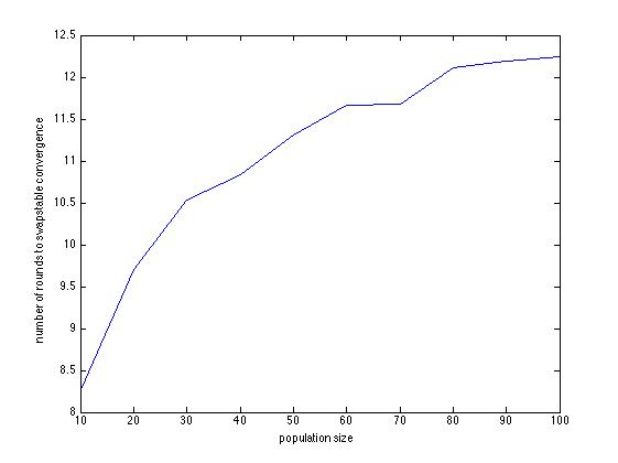
Figure 8: Average number of rounds for swapstable convergence vs. $n$, for $C_{\textrm{E}}=C_{\textrm{I}}=2$.

The first question that arises in the consideration of any kind of best response dynamic is whether and how quickly it will converge to the corresponding equilibrium notion. Interestingly, empirically it appears that swapstable best response dynamics always converges rather rapidly. In Figure 8 we show the average number of rounds to convergence over many trials, starting from dense initial connectivity (average degree 5), for varying values of $n$. The growth in rounds appears to be strongly sublinear in $n$ (recall that each round updates all $n$ players, so the overall amount of computation is still superlinear in $n$). Thus we conjecture the general and fast convergence of swapstable dynamics. See Appendix G for more details.

In Section 3, we gave a number of formal examples of Nash and swapstable equilibria with respect to the maximum carnage adversary. These examples tended to exhibit a large amount of symmetry, especially those containing cycles, due to the large number of cases that need to be considered in the proofs. Figure 9 shows a sampling of “typical” equilibria found via simulation for $n=50$, which exhibit interesting asymmetries and illustrate the effects of the parameters.

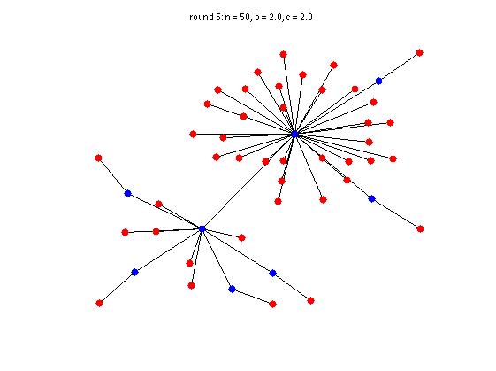
Figure 9: Sample equilibria reached by swapstable best response dynamics for $n=50$. Left: $C_{\textrm{E}}=0.5$, $C_{\textrm{I}}=2$. Middle: $C_{\textrm{E}}=2$, $C_{\textrm{I}}=2$. Right: $C_{\textrm{E}}=0.5$, $C_{\textrm{I}}=20$.

In the left panel of Figure 9, $C_{\textrm{E}}=0.5$ and $C_{\textrm{I}}=2$. Thus players have an incentive to buy edges even to isolated vertices as long as they do not increase their vulnerability to the attack. In this regime, despite the initial disconnectedness of the graph, we often see equilibria with a long cycle (as shown), with various tree-like structures attached. In the middle panel we left $C_{\textrm{I}}=2$ but increased $C_{\textrm{E}}$ to 2. In this regime cycles are less common due to the higher $C_{\textrm{E}}$. The equilibrium illustrated is a tree formed by a connected “backbone” of immunized players, each with varying numbers of vulnerable children. Finally, in the right panel we return to inexpensive edges ($C_{\textrm{E}}=0.5$), but greatly increased $C_{\textrm{I}}$ to 20. In this regime, we see fragmented equilibria with no immunizations. We note that unlike the right example which is trivial, the examples in the left and middle are non-trivial equilibria with high social welfare as predicted by theory.

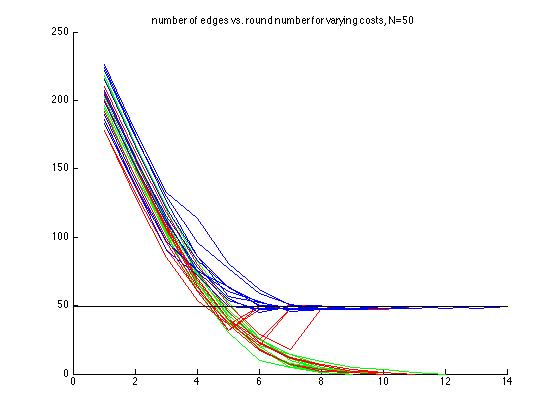
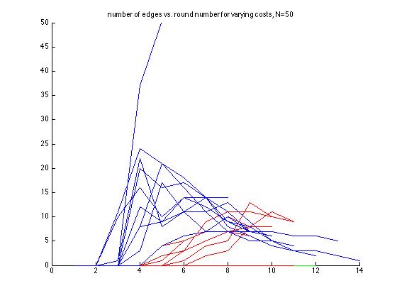
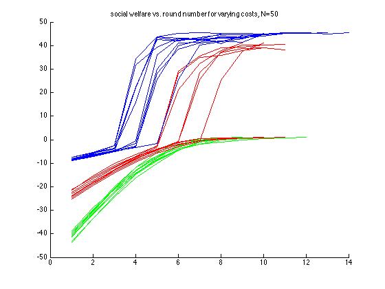
Figure 10: Number of edges (left panel), number of immunizations (middle panel), and average welfare (right panel) vs. number of rounds, for $N=50$ and varying values for $C_{\textrm{I}}$ and $C_{\textrm{E}}$. See text for discussion.

Figure 9 provides snapshots only at the conclusion of swapstable dynamics while Figure 10 examines entire paths, again at $n=50$. We started from denser initial graphs (average degree 5), and each panel visualizes a different quantity per number of rounds, for 3 cost regimes: inexpensive cost $C_{\textrm{E}}=C_{\textrm{I}}=2$ (blue); moderate cost $C_{\textrm{E}}=C_{\textrm{I}}=6$ (red); and expensive cost $C_{\textrm{E}}=C_{\textrm{I}}=10$ (green). In each panel there are 10 simulations for each cost regime.

In the left panel, we show the evolution of the total number of edges ($y$ axis) in the graph over successive rounds ($x$ axis). In all regimes, there is initially a precipitous decline in connectivity, as the overly dense initial graph cannot be supported at equilibrium. So in the early rounds all players are dropping edges. The ultimate connectivity, however, depends on the cost regime. In the inexpensive regime, connectivity falls monotonically until it levels out very near the threshold for global connectivity at $n-1$ (horizontal black line), resulting in trees or perhaps just one cycle. In the moderate regime, we see a bifurcation; in some trials, connectivity fall all the way to the empty graph at equilibrium, while in others fall well below the $n-1$ tree threshold, but then “recover” back to that threshold (which we discuss shortly). In the expensive regime, all trials again result in a monotonic fall of connectivity all the way to the empty graph.

For the same cost regimes and trials, the middle panel shows the number of immunizations purchased over successive rounds. In the inexpensive regime, immunizations, sometimes many, are purchased in early rounds. These act as a “safety net” that prevents connectivity from falling below the tree threshold. Typically immunizations grow initially and then decline. In the moderate regime, we see that the explanation for the connectivity bifurcation discussed above can be traced to immunization decisions. In the trials where connectivity is recovered, some players eventually choose to immunize and thus provide the focal points for edge repurchasing. In many trials resulted in the empty graph, immunizations never occurred (these remain at $y=0$). In the expensive regime, no trials are visible because immunizations are never purchased.

Finally, the right panel shows the evolution of the average social welfare per player over successive rounds. In the inexpensive regime, welfare increase slowly and modestly from negative values in the initial graph, then increase dramatically as the benefits of immunization are realized. In the moderate regime, we see a bifurcation of welfare corresponding directly to the bifurcation of connectivity. In the expensive regime, all trials converge from below to the minimum (1-$1/n$) welfare of the empty graph. Again as theory suggested, the relationship between $C_{\textrm{E}},C_{\textrm{I}}$ and $n$ is determining whether convergence is to a non-trivial equilibrium and thus high social welfare, or to a highly fragmented network with no immunizations and low social welfare.

We conclude by noting that for many parameters, the dynamics above result in heavy-tailed degree distributions — a property commonly observed in large-scale social networks that is easy to capture in stochastic generative models (such as preferential attachment), but more rare in strategic network formation. Across 200 simulations for $n=100$, $C_{\textrm{E}}=0.5$ and $C_{\textrm{I}}=2$, we computed the ratio of the maximum to the average degree in each equilibrium found. The lowest, average and maximum ratio observed were 6, 15.8, and 41, respectively (so the highest degree is consistently an order of magnitude greater than the average or more). Moreover, in all 200 trials the highest-degree vertex chose immunization, despite the average rate of immunization of 23% across the population. Thus an amplification process seems to be at work, where vertices that immunize early become the recipients of many edge purchases, since they provide other vertices connectivity benefits that are relatively secure against attack without the cost of immunization.

7 A Behavioral Experiment

To complement our theory and simulations, we conducted a behavioral experiment on our game with 118 participants. The participants were students in an undergraduate survey course on network science at the University of Pennsylvania. As training, participants were given a detailed document and lecture on the game, with simple examples of payoffs for players on small graphs under various edge purchase and immunization decisions. (See http://www.cis.upenn.edu/~mkearns/teaching/NetworkedLife/NetworkFormationExperiment2015.pdf for the training document provided to participants.) Participation was a course requirement, and students were instructed that their grade on the assignment would be exactly equal to their payoffs according to the rules of the game. Students thus had strong motivation to think carefully about the game. There was a 2-day gap between the training lecture and the experiment, so subjects had time to contemplate strategies; they were instructed not to discuss the experiment with each other during this period, and that doing so would be considered cheating on the assignment.

We again focused on the maximum carnage adversary in this section. Also costs of $C_{\textrm{E}}=5$ and $C_{\textrm{I}}=20$ were used for the following twofold reasons. First, with $n=118$ participants (so a maximum connectivity benefit of 118 points), it felt that these values made edge purchases and immunization significant expenses and thus worth careful deliberation. Second, running swapstable best response simulations using these values generally resulted in non-trivial equilibria with high welfare, whereas raising $C_{\textrm{E}}$ and $C_{\textrm{I}}$ significantly generally resulted in empty or fragmented graphs with low welfare.

In a game of such complexity, with so many participants, it is unreasonable and uninteresting to formulate the experiment as a one-shot simultaneous move game. Rather, some form of communication must be allowed. We chose to conduct the experiment in an open courtyard with the single ground rule that all conversations be quiet and local i.e. in order to hear what a participant was saying to others, one should have to stand next to them. The goal was to permit communication amongst small groups of participants but to prevent global coordination via broadcasting. The “quiet rule” was enforced by several proctors for the experiment.

Figure 11: Experiment participants gathered quickly in small groups that reformed frequently during the experiment.

Other than the quiet rule, participants were told there were no restrictions on the nature of conversations. In particular, they were free to enter agreements, make promises or threats and move freely in the courtyard. However, it was also made clear to them that any agreements or bargains struck would not be enforced by the rules of the experiment and thus were non-binding. Each subject was given a handout that simply required them to indicate which other subjects they chose to purchase edges to (if any), and whether or not they chose to purchase immunization. The handout contained a list of subject names, along with a unique identification number for each subject that was used to indicate edge purchases. Thus subjects knew the actual names of the others as well as their assigned ID numbers. An entire class session was devoted to the experiment, but subjects were free to (irrevocably) turn in their handout at any time and leave the experiment. Thus subjects committed to their actions and exited sequentially, and the entire duration was approximately 30 minutes. During the experiment, subjects tended to gather quickly in small discussion groups that reformed frequently, with subjects moving freely from group to group. (See Figure 11). It is clear from the outcome that despite adherence to the quiet rule, the subjects engaged in widespread coordination via this rapid mixing of small groups.

In the left panel of Figure 12, we show the final undirected network formed by the edge purchases and immunization decisions. The graph is clearly anchored by two main immunized hub vertices, each with many spokes who purchased their single edge to the respective hub. These two large hubs are both directly connected, as well as by a longer “bridge” of three vulnerable vertices. There is also a smaller hub with just a handful of spokes, again connected to one of the larger hubs via a chain of two vulnerable vertices.

In terms of the payoffs, inspection of the behavioral network reveals that there are two groups of three vertices that are the largest vulnerable connected components, and thus are the targets of the attack. These 6 players are each killed with probability $1/2$ for an expected payoff that is only half that of the wealthiest players (the vulnerable spokes of degree 1). In between are the players who purchased immunization including the three hubs as well as two immunized spokes. The immunized spoke of the upper hub is unnecessarily so, while the immunized spoke in the lower hub is in fact best responding — had they not purchased immunization, they would have formed a unique largest vulnerable component of size 4 and thus been killed with certainty.

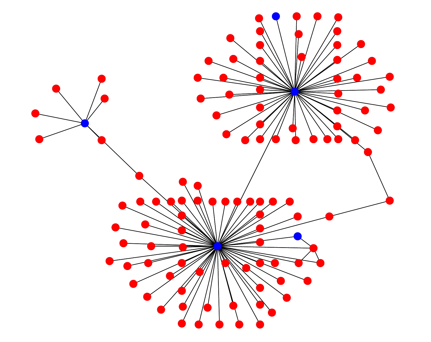
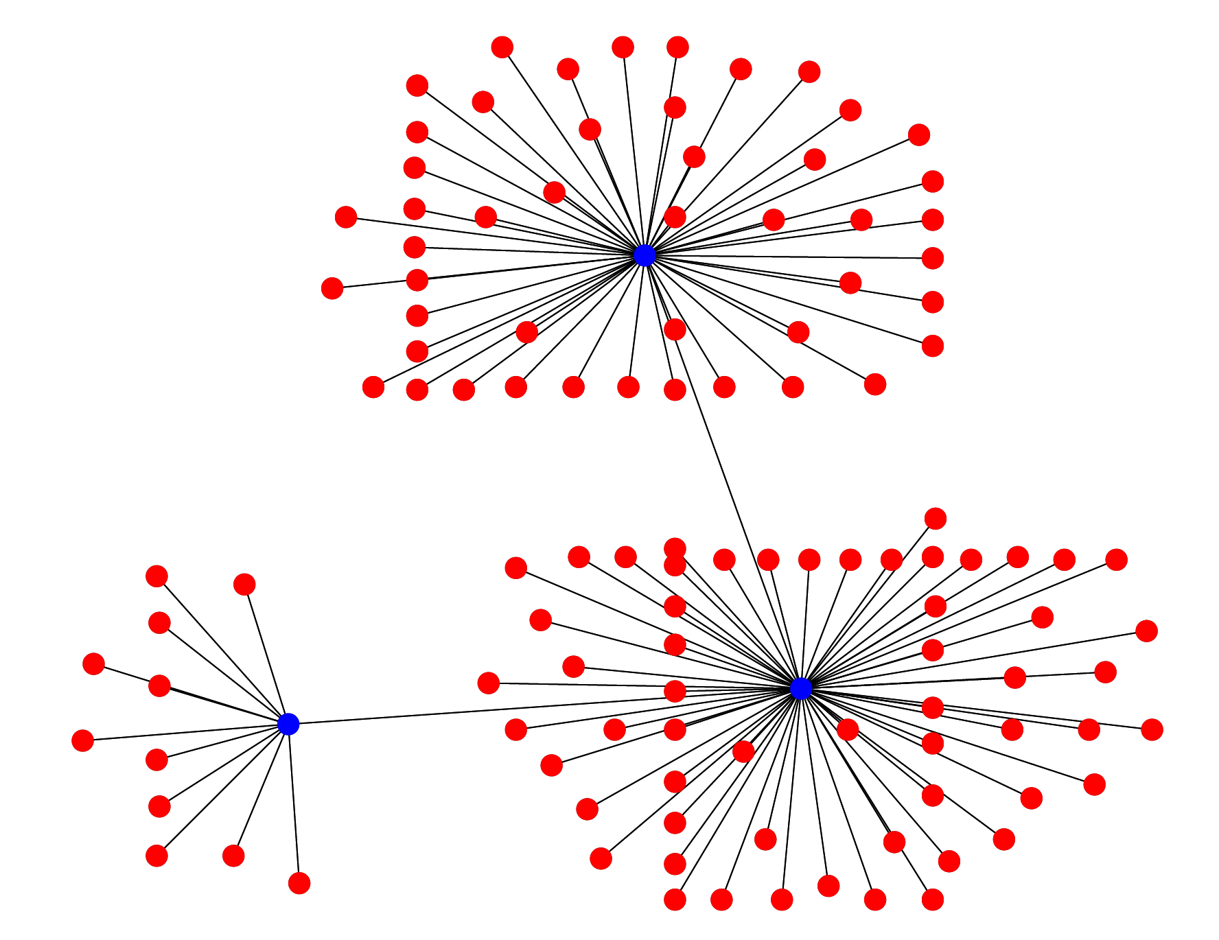
Figure 12: Left: the final undirected network formed by the edge purchases and immunization decisions (blue for immunized, red for vulnerable). Right: a “nearby” Nash network.

It is striking how many properties the behavioral network shares with the theory in Sections 4 and 5 and the simulations in Section 6: multiple hub-spoke structures with sparse connecting bridges, resulting in high welfare and a heavy-tailed degree distribution; a couple of cycles; and multiple targeted components. We can quantify how far the behavioral network is from equilibrium by using it as the starting point for swapstable best response dynamics and running until convergence. In the right panel of Figure 12, we show the resulting Nash network reached from the behavioral network in only 4 rounds of swapstable dynamics, and with only 15 of 118 vertices updating their choices. The dynamics simply “clean up” some suboptimal behavioral decisions — the vulnerable bridges between hubs are replaced by direct edges, the other targeted group of three spokes drops theirs fatal edges, and immunizing spokes no longer do so.

Participants were also required to complete an email survey shortly after the experiment, in which they were asked to comment on any strategies they contemplated prior to the experiment; whether and how those strategies changed during the experiment; and what strategies or behaviors they observed in other participants. The responses to these surveys are quite illuminating regarding both individual and collective behavior. We point out some of these responses in the rest of this section.

Many subjects reported entering the experiment with not just a strategy for their own behavior, but in fact some kind of “master plan” they hoped to convince others to join. One frequently reported master plan involved variations on simple cycles:

• Going into the experiment my goal was to have everyone connect with one another and take the immunity in a circle.

• I tried to create a cycle to start. Then I wanted to convince everyone to join our cycle. I figured this would work well because if any of us got immunity it would decrease the probability of being infected.

Interestingly, little thought seems to have been given to how to actually quickly coordinate a global ordering of the participants in a cycle via only quiet conversation in small groups.

Another frequently cited plan involved the hub and spoke structure that was largely realized:

• I thought about the possibility of everybody in the class connecting to one person and that person getting immunized.

• I thought of the hub and spoke model with a hub being immunized. If everyone agreed to this plan then one individual would take a 20 point hit, and every other player would take a 5 +(x-1)/x*number of vertices in component hit. This would maximize everyone’s points. Thankfully we had some volunteers to make use of this method. I believe if everyone did as they should, then we will all have our maximum scores.

The strategies above are largely based on mathematical abstractions, but others reported planning to use real-world social relationships in their strategies:

• Beforehand, I planned to connect to other students that I knew personally, to have around 3-4 connections. As well, I was going to make one long-distance “random edge” to increase the size/diversity of my component.

• I thought of trying to connect with the decently large group of friends who sat in front as well as one or two other random people and then giving myself immunity in order to ensure that I would be safe if the large component I was connected to got compromised by the virus.

• Before the experiment my strategy was to create a cycle with my friends in the class and then connect with one person that has immunity [who] could potentially connect me with another component.

• Being a freshman, and knowing that the freshman class of NETS is pretty tight-knit I thought that it would be a good idea to choose someone from that freshman group, because I thought that the component would be of a decent size, but not the giant component itself.

Of course, of particular interest are the surveys of the two large hubs, one of whom was male (who we shall thus refer to as Hub M, and had ID number 128) and the other female (Hub F, ID number 127). Hub F reports:

The idea was that there would be one hub, with immunity, that everyone would connect to. This seemed like the best idea, because any other idea would pit communities against each other, and the highest payoff that could be expected from any fight between communities would be 49%. I was willing to be the hub with a lower score of n-20 so everyone else could get a score of (n-1/n)(n-5) rather than have everyone fight… I went to my friends and told them to spread the word for no one to buy immunity and for everyone to put down 127 as the only person to whom they’d connect, and explained to my friends my reasoning so they could explain to everyone else. A few minutes in, I realized someone else had had the same idea as me (conveniently, number 128) and so I had to adapt my plan because so many people had already put down 128… We decided to team up and connect with each other, and both opt for immunity, because that would give us the same results as we’d both originally intended. Technically, only one had to connected to the other, and originally, 128 connected with me, but I decided for diplomatic reasons to connect back, so that it would be somewhat more fair to both sides… A few people who approached me and 128 ended up switching from 128 to me because, apparently, “girls are more trustworthy”.

Hub F thus seems to report an altruistic motivation for purchasing immunization, hoping to maximize social welfare. In contrast, Hub M displays a more Machiavellian attitude:

I planned to form a radial network with one person being at the center and all other people will connect to this person and this person only. And this person at the central position will buy vaccine and no edges… However, the catch of this strategy is that the person at the center will score at least 15 points lower than all other nodes that surround him or her. Assuming that the end result is curved, I theorized that if we partition all the NETS students into two groups, those who are inside this radial network (Group A) and those who are not (Group B). The person at the center will still be better off… the person at the center of the radial network will not end up being the last person in the class and will achieve a decent score by absolute value (thus there will be less of a disincentive for him to be at the center).

Thus Hub M was willing to immunize in the hopes of actually creating three distinct groups of participants: the “winners” who would connect to Hub M; Hub M himself, with slightly lower payoff; and then a large group of “losers” who would be deliberately left out of the immunized hub and spoke structure.

It is clear from the surveys that word quickly spread during the experiment to connect to Hubs F and M, and that many participants joined this strategy — though not without some reported mistrust, hesitation and manipulation:

• Some bought in immediately, some are skeptical. Nature of the conversation is usually about: is the person in the middle going to keep the his promise? What if he screws everyone else?

• During the experiment I tried to convince as many people as possible to connect with me. I lied about how many people I was actually connected with.

• Something I found interesting with this experiment was how people found ways to create artificial trust in others. Something that I myself did and something that others did as well, was to put trust in number 127 by saying that since she marked her paper in pen, circling the option to buy immunity we could trust her. She very easily could have crossed that option off later, the fact that she used pen doesn’t mean she for sure was trustworthy, but it is comforting to find a way to trust someone and that was one of the strategies that people, including myself, used. Other ways I overheard others create artificial trust was by saying, lets mark 127 or 128 based on their gender. Some girls marked 127 because she was a girl and some guys marked 128 because he was a guy.

Finally, perhaps the most poignant remarks came from the participant who was responsible for creating one of the two targeted components, only realizing so in hindsight:

I missed the collaboration part of the experiment where the entire class came up with a plan so I pretty much used a similar strategy to what I had previously thought up. I wrote down the name of the girl in my main group (that would have created a chain) and then wrote down two other people that would be my “random” connections. However, I didn’t get immunity because I assumed that one of the three people I had connected to bought immunity… Upon speaking with someone else about my strategy, I saw how flawed it was. They explained to me what the class had done… there is a high chance that I may have killed myself and the three people I connected to. If the three people I connected to die, it is because I did not buy immunity. If they die, it will be my fault — not theirs. I regret implementing my strategy.

8 Discussion and Future Work

We mention some areas for further study. Within our model, the question of whether swapstable best response provably converges (as seen empirically) is open. The benefit function considered here is one of many possible natural choices. It would be interesting to consider other functions. Another extension includes imperfect immunization which fails with some probability e.g. as a function of the amount of investment.

We mention two natural variants. The first is the combination of our original model with a standard diffusion model for the spread of attack. For example, combining with the independent cascade model [19], when a targeted vertex is attacked, the infection spreads with probability $p$ along the edges from the attacked point for which both endpoints are unimmunized. This spread then continues until we reach immunized vertices which again act as firewalls. Again different adversaries can have different objectives e.g. the maximum carnage adversary will pick an attack point which maximizes the expected spread. Wang et al. [25] showed that computing the spread in the independent cascade model is #P-complete. This suggests that even before considering the complexity of analysis, agents’ reasoning about the choice of attack by the adversary can become quite complicated. Furthermore, due to the probabilistic nature of the spread, it is nontrivial to establish any sparsity properties of the equilibria, because additional overbuilding might occur to hedge against uncertainty of how the infection will spread. Welfare is yet more difficult to analyze; unlike the deterministic spread, it is no longer obvious that a vertex likely to end up in a small component post-attack has a single fixed edge purchase that would greatly improve her utility, since different spread patterns can disconnect her from different regions.

The second variant is identical to our current model except that it requires edge purchases to be bilateral. In this variant, the concept of equilibrium might be replaced by the notion of pairwise stability (see e.g. [16]). As a majority of our results hinge upon the analysis of unilateral deviations, our current analysis cannot be easily modified to accommodate this change. As a first step towards this goal, the game we study could be modified by adding a blocking action with 0 cost while maintaining the unilateral edge formation. Namely for any edge purchased from player $i$ to $j$, player $j$ can block the edge with no cost. The blocking action removes both the potential connectivity benefit or risk of contagion from edge $(i,j)$ for both $i$ and $j$. The first observation is that there are equilibrium networks in our game which are not equilibria in this new game with blocking. Moreover, we can show that in any equilibrium of the new game, no player blocks any of edges purchased to her. Finally we can show that all the properties of our game (sparsity, connectivity and social welfare) hold in the new game with blocking as well.

APPENDIX

Appendix A Difference Between Solution Concepts

As we mentioned in Section 2, linkstable equilibria and swapstable equilibria are both generalizations of Nash equilibria. In particular, this implies that any Nash equilibrium is also a swapstable and linkstable equilibrium. Furthermore, since linkstable equilibria is also a generalization of swapstable equilibria, then any swapstable equilibrium is also a linkstable equilibrium.

In this section we show that these solutions concepts are in fact different in our game. To do so, we focus on the maximum carnage adversary. We first show an example of a swapstable equilibrium with respect to the maximum carnage adversary which is not a Nash equilibrium (Example 1). We then show an example of a linkstable equilibrium maximum carnage adversary which is neither a swapstable equilibrium nor a Nash equilibrium (Example 2).

First, we state the following useful Lemma.

Lemma 4.

Let $G=(V,E)$ be a Nash, swapstable or linkstable equilibrium network with respect to the maximum carnage adversary. The number of targeted regions cannot be one when $|V|>1$.

Proof.

Suppose by contradiction that there exists only one targeted region $\mathcal{T}$. Then $\mathcal{T}$ must be a singleton vertex; otherwise, some player in $\mathcal{T}$ must have purchased an edge and the utility of this player is negative as the attack uniquely targets $\mathcal{T}$ (killing it with probability $1$). Let $u$ denote the singleton vertex in $\mathcal{T}$. Then the expected utility of $u$ is 0, and neither $u$ nor any other vertex will purchase an edge incident to $u$.

Now since the number of vertices is strictly bigger than 1, there exists some other vertex $v\in V$; this other vertex (and any other vertices besides $u$) must be immunized since $\mathcal{T}$ (which is a singleton) is the unique targeted region. First suppose that $G$ is the empty graph (i.e., $E=\emptyset$), then for $v$’s behavior to be a best response, it must be that $C_{\textrm{I}}\leq 1/2$, since she could drop her immunization for expected payoff $1/2$ rather than her current expected payoff of $1-C_{\textrm{I}}$. Then, $u$’s expected payoff after immunizing would be $1-C_{\textrm{I}}\geq 1/2>0$, higher than her current expected payoff; a contradiction to $G$ being an equilibrium. Now suppose $G$ is not an empty graph. So there is some immunized vertex $v\in V\setminus\{u\}$ who purchases an edge to some other $v^{\prime}\in V\setminus\{u,v\}$. Let $B$ denote the connected component in $G$ that contains $v,v^{\prime}$. Since $v$ is best responding, it must be that $|B|-C_{\textrm{I}}-C_{\textrm{E}}\geq 1/2$, since $v$ could have chosen to not buy and edge to $v^{\prime}$ and not to immunize for an expected utility of at least $1/2$. This implies that $u$ cannot be best responding in this case, since buying an edge to $v$ and immunizing would give $u$ an expected utility of $(|B|+1)-C_{\textrm{I}}-C_{\textrm{E}}\geq 3/2>0$, a contradiction to $G$ being an equilibrium. ∎

We then show that the set of swapstable equilibria is indeed larger than the set of Nash equilibria in our game (see Figure 13).

Figure 13: An example of swapstable equilibrium with respect to the maximum carnage adversary which is not a Nash equilibrium. $C_{\textrm{E}}=1$ and $C_{\textrm{I}}=4$.

Example 1.

Let $n=3k$ and consider $k$ disjoint trees of size $3$. In each tree, there exists a root vertex that both other vertices purchase an edge to the root. When $c\in(0,3/2)$, $C_{\textrm{I}}\in[4,6]$ and $k\geq 9$, the mentioned network is a swapstable equilibrium with respect to the maximum carnage adversary but is not a Nash equilibrium.

Proof.

Due to the symmetry in this network, we only need to consider the deviations for two types of vertices: the root vertex, and the vertex that purchases an edge to the root.

Let’s consider the root vertex first. Her utility is $3(1-1/k)$ and her swapstable deviations are as follows:

1. adding one edge.

2. adding one edge and immunizing.

3. immunizing.

We show that none of these deviations are beneficial by showing that the utility before the deviation is always (weakly) bigger than the utility after deviation.

Case 1 trivially does not happen, because if the root adds an edge to a different tree, she would be a part of the unique targeted region which cannot happen in any equilibrium by Lemma 4. She also does not want to purchase an edge to any other vertex in her tree, since she is connected to all the other vertices already.

In case 2, she will survive with probability 1 after immunization. As far as the edge purchasing decision, she would get the maximum utility if she purchases an edge to a different tree.

$$C_{\textrm{I}}\geq 4\text{ and }C_{\textrm{E}}\geq 0\implies C_{\textrm{I}}+C_{\textrm{E}}\geq 4\text{ and }k\geq 9\implies$$

$$3\left(1-\frac{1}{k}\right)\geq\left(3+3(1-\frac{1}{k-1})\right)-C_{\textrm{E}}-C_{\textrm{I}}.$$

In case 3, she will survive with probability one but she has to pay for immunization.

$$C_{\textrm{I}}\geq 4\text{ and }k\geq 9\implies 3(1-\frac{1}{k})\geq 3-C_{\textrm{I}}.$$

Next, consider a vertex that purchased an edge. Such vertex has a utility of $3(1-1/k)-C_{\textrm{E}}$ and her swapstable deviations are as follows:

1. dropping her purchased edge.

2. dropping her purchased edge and immunizing.

3. adding one more edge.

4. adding one more edge and immunizing.

5. immunizing.

6. swapping her edge.

7. swapping her edge and immunizing.

We again show that none of these deviations are beneficial.

In case 1, she would survive with probability 1 after dropping her edge but the size of her connected component will also decrease.

$$C_{\textrm{E}}\in(0,\frac{3}{2})\text{ and }k\geq 9\implies 3(1-\frac{1}{k})-C_{\textrm{E}}\geq 1.$$

In case 2, once she drops her purchased edge, she is no longer a targeted vertex. So immunization has no benefits in this case and as long as case 1 is not beneficial, case 2 cannot be beneficial either.

The analysis of Case 3 is exactly the same as the analysis of case 1 of the root vertex.

In case 4, she will survive with probability 1 after immunization. As far as the edge purchasing decision, she would get the maximum utility if she purchases an edge to a different tree.

$$C_{\textrm{I}}\geq 4\text{ and }C_{\textrm{E}}\geq 0\implies C_{\textrm{I}}+C_{\textrm{E}}\geq 4\text{ and }k\geq 9$$

$$\implies 3(1-\frac{1}{k})-C_{\textrm{E}}\geq\left(3+3(1-\frac{1}{k-1})\right)-2\cdot C_{\textrm{E}}-C_{\textrm{I}}.$$

In case 5, she will survive with probability one but she has to pay for immunization which is costly.

$$C_{\textrm{I}}\geq 4\text{ and }k\geq 9\implies 3(1-\frac{1}{k})-C_{\textrm{E}}\geq 3-C_{\textrm{E}}-C_{\textrm{I}}.$$

In case 6, swapping her purchased edge to a vertex in another tree will cause her to be a part of the unique targeted region which cannot happen in any equilibrium by Lemma 4. Also, obviously, swapping to another vertex in her tree will leave her utility unchanged.

In case 7, swapping her purchased edge to a vertex in the same tree and immunizing is not beneficial as long case 5 is not beneficial (she has the same expenditure and benefit as in case 5). So we only need to consider the case when she swaps her edge to a vertex in a different tree and immunizes.

$$C_{\textrm{I}}\geq 4\implies 3(1-\frac{1}{k})\geq\left(1+3(1-\frac{1}{k})\right)-C_{\textrm{I}}.$$

Finally, it is easy to come up with a strictly beneficial Nash deviation which implies that the above network is not a Nash equilibrium with respect to the maximum carnage adversary. Consider any vertex that did not purchase an edge. She has a utility of $3(1-1/k)$. Consider her utility when she buys one edge to all the other trees and immunizes herself.

$$C_{\textrm{I}}\leq 5\text{ and } k\geq 9\text{ and }C_{\textrm{E}}\leq\frac{3}{2}<2\implies$$

$$(3k-3)-C_{\textrm{E}}\cdot(k-1)-C_{\textrm{I}}\geq(3k-3)-2(k-1)-5=k-6\geq 3.$$

So her utility strictly increases by this deviation, implying that such network cannot be a Nash equilibrium. ∎

Finally, we show that the set of linkstable equilibria is indeed larger than the set of swapstable equilibria (which itself is larger than the set of Nash equilibria). See Figure 14.

Figure 14: An example of linkstable equilibrium with respect to the maximum carnage adversary which is not a swapstable equilibrium. $C_{\textrm{E}}=2$ and $C_{\textrm{I}}=4$.

Example 2.

Consider a cycle consisting of $n=3k$ vertices. If (i) every player buys the edge in her counter clockwise direction on the cycle, (ii) every third vertex in the cycle immunizes (so there are $k$ immunized vertices in the cycle) and (ii) $C_{\textrm{E}}\in(0,n/2-5),C_{\textrm{I}}\in(3,n/2+3)$ and $k\geq 7$, then the cycle is a linkstable equilibrium with respect to the maximum carnage adversary but not a swapstable equilibrium.

Proof.

First, consider any immunized vertex. This vertex clearly cannot change her immunization, regardless of how she changes her edge purchases. Since she is always connected to the vulnerable vertex to her counter clockwise direction, changing the immunization, will result in forming the unique largest targeted region which by Lemma 4 cannot happen in any equilibrium. So as long as the payoff of the immunized vertex is greater than zero before the deviation, she will not change her immunization decision.

$$C_{\textrm{E}}<\frac{n}{2}-5\text{ and }C_{\textrm{I}}<\frac{n}{2}+3\implies C_{\textrm{E}}+C_{\textrm{I}}<n-2\implies(n-2)-C_{\textrm{E}}-C_{\textrm{I}}>0.$$

Furthermore, fixing the immunization decision, the linkstable edge purchasing deviations for any of the immunized vertices are as follows.

1. adding one more edge.

2. dropping her purchased edge.

In each case we consider the utilities after and before the deviation and show that given the conditions in the statement of the example, the deviation in not beneficial.

In case 1, before the deviation the immunized vertex remains connected to any vertex that survives. So adding more edges will only increase the expenditure while the connectivity benefit is the same. Since $C_{\textrm{E}}>0$, this deviation is not beneficial.

In case 2, dropping her edge might cause the network to become disconnected after the attack and, hence, it decreases the connectivity benefit of the vertex.

$$C_{\textrm{E}}<\frac{n}{2}-5<\frac{n}{2}-\frac{3}{2}=\frac{3}{2}(k-1)\implies(n-2)-C_{\textrm{E}}-C_{\textrm{I}}>\frac{1}{k}\Big{(}1+4+\ldots+\left(3k-2\right)\Big{)}-C_{\textrm{I}}.$$

Now, we consider the vulnerable vertices. Any such vertex (if survives) will remain connected to any other survived vertex. So no vulnerable vertex wants to add more edges (while keeping her purchased edge). So the possible deviations of such vertices that we need to consider are as follows.

1. immunizing.

2. dropping her purchased edge.

3. dropping her purchased edge and immunizing.

Similar to the case of the immunized vertex, we compare the utilities after and before the deviation and show that given the conditions in the statement of the example, the deviation is not beneficial.

We divide the vulnerable vertices into two disjoint categories: (i) one that purchases an edge to an immunized vertex (type i) and (ii) one that purchases an edge to a vulnerable vertex (type ii). For the 2nd and 3rd deviation, we need to distinguish between these two types.

In case 1, the vertex who immunizes survives. Also her vulnerable neighbor is not targeted anymore.

$$C_{\textrm{I}}>3 \implies C_{\textrm{I}}>3-\frac{6}{n}=3-\frac{2}{k}\implies(1-\frac{1}{k})(n-2)-C_{\textrm{E}}>(n-2)-C_{\textrm{E}}-C_{\textrm{I}}.$$

In case 2, dropping her edge might cause the network to become disconnected after the attack and, hence, it decreases the connectivity benefit of the vertex. For a type i vertex,

$$C_{\textrm{E}}<\frac{n}{2}-5<\frac{n}{2}-\frac{7}{2}+\frac{6}{n}\implies(1-\frac{1}{k})(n-2)-C_{\textrm{E}}>\frac{1}{k}\Big{(}3+6+\ldots+(3k-3)\Big{)}.$$

For a type ii vertex, the analysis is slightly different since after dropping her purchased edge, the vertex will not be a part of any targeted region anymore.

$$C_{\textrm{E}}<\frac{n}{2}-5<\frac{n}{2}-4+\frac{6}{n}\implies(1-\frac{1}{k})(n-2)-C_{\textrm{E}}>\left(2+\frac{1}{k-1}\Big{(}0+3+6+\ldots+(3k-6)\Big{)}\right).$$

In case 3, a type i vertex always survives if she immunizes but dropping the edge will decrease her connectivity benefit.

$$C_{\textrm{E}} <\frac{n}{2}-5\text{ and }C_{\textrm{I}}>3\implies C_{\textrm{E}}-C_{\textrm{I}}<\frac{n}{2}-8<\frac{n}{2}-5+\frac{6}{n}$$

$$\implies(1-\frac{1}{k})(n-2)-C_{\textrm{E}}>\frac{1}{k-1}\Big{(}3+6+\ldots+\left(3k-3\right)\Big{)}-C_{\textrm{I}}.$$

Note that a type ii vertex survives if she drops her edge. So immunization will only increase her expenditure. So a type ii vertex always prefers the deviation in case 2 to the deviation in case 3. And since we showed that the deviation in case 2 is not beneficial for a type ii vertex, the deviation in case 3 cannot be beneficial either.

Now it is easy to see that this network cannot form in any swapstable equilibrium. Consider two vulnerable vertices (denoted by $u$ and $v$) that are connected to each other with an edge. Suppose without loss of generality that $u$ has purchased the edge between $u$ and $v$. Now, it is to see that $u$ can get a strictly higher payoff by dropping the edge purchased to $v$ and instead buying an edge to the immunized vertex that $v$ is connected to. This way, $u$ is not a part of any targeted region anymore (so she survives with probability $1$ instead of $1-1/k$) but she is still connected to every vertex she was connected to before the deviation. Since her expenditure is exactly the same this deviation will increase her utility and show that such network cannot form in any swapstable equilibrium. ∎

Appendix B Comparison of Different Attack Models

Throughout we showed that the equilibrium networks in the three stylized models introduced in Section 2 exhibit similar behaviors regarding sparsity and welfare. So in this section we ask whether the equilibrium networks in these models are the same? We answer this question negatively. In particular, in Example 3 we show that there exist (connected) Nash equilibrium networks with respect to the maximum disruption adversary that are not equilibria with respect to the maximum carnage adversary. We then in Example 4 show that there exist (connected) Nash equilibrium networks with respect to the maximum carnage adversary that are not equilibria with respect to the maximum disruption adversary. While we can also show the set of equilibrium networks with respect to the random attack adversary is also disjoint from the the set of equilibrium networks with respect to the other two adversaries, we omit the details due to similarities.

Example 3.

There exists a Nash equilibrium network with respect to the maximum disruption adversary which is not a Nash equilibrium with respect to the maximum carnage adversary.

Proof.

Consider a complete binary tree with $n=2^{n^{\prime}+1}-1$ vertices (so the height of the tree is $n^{\prime}$). Suppose every player in height $i>0$ buys the two edges to the players in height $i-1$ and every vertex in height $i>0$ immunizes (see Figure 15). Then for $C_{\textrm{I}}\in(2,n-2)$, $C_{\textrm{E}}\in(0,1-1/2^{n^{\prime}})$ and $n^{\prime}\geq 3$ this tree is a Nash equilibrium with respect to the maximum disruption adversary but not with respect to the maximum carnage adversary.

Figure 15: An example of Nash equilibrium with respect to the maximum disruption adversary which is not a Nash equilibrium with respect to the maximum carnage adversary. $C_{\textrm{E}}=15/16$ and $C_{\textrm{I}}=33/16$.

We first show that the tree in Figure 15 is an equilibrium with respect to the maximum disruption adversary. First, consider any immunized vertex other than the root of the tree. If such vertex changes her immunization decision (regardless of how she changes her edge purchasing decision), she would deterministically get killed by the maximum disruption adversary. So she would not change her immunization decision as long as her utility is positive which means $(n-1)-C_{\textrm{I}}-2C_{\textrm{E}}>0$. The same applies to the root as long as the root maintains one of her purchased edges. It is easy to see that the deviation that she drops both of her edges and changes her immunization is also not beneficial as long as $(n-1)-C_{\textrm{I}}-2C_{\textrm{E}}>1$ since she would not get attacked by the adversary in this case.

Any vertex who survives after an attack will remain connected to any other surviving vertex; which implies no vertex would strictly prefer to add another edge. We now show that no vertex would like to drop any of her purchased edges and leaf vertices in height 0 would prefer to remain targeted. To show the former, note that the benefit from each edge purchase is at least $1-1/2^{n^{\prime}}$ and this comes from edges purchased to the targeted leaves. So no vertex would prefer to drop any of her edges since the benefit is strictly more than $C_{\textrm{E}}$. To show the latter, the utility of a leaf in the tree is $(1-1/{2^{n^{\prime}}})(n-1)$. If she immunizes her connectivity benefit would become $n-1$ but she has to pay a price of $C_{\textrm{I}}$ which is strictly higher than $(n-1)/2^{n^{\prime}}$. So no leaf vertex would prefer to immunize.

To show that the tree in Figure 15 is not a Nash equilibrium with respect to the maximum carnage adversary, we show that any vertex in height 2 can strictly increase her utility by changing her immunization. Her utility before the deviation is $(n-1)-2C_{\textrm{E}}-C_{\textrm{I}}$ and her utility after the deviation is $(1-1/(2^{n^{\prime}}+1))(n-1)-2C_{\textrm{E}}$. So as long as $C_{\textrm{I}}>(n-1)/(2^{n^{\prime}}+1)=2^{n^{\prime}+1}/(2^{n^{\prime}}+1)=2-2/(2^{n^{\prime}}+1)$, then this deviation is beneficial for a height 2 vertex. ∎

Example 4.

There exists a Nash equilibrium network with respect to the maximum carnage adversary which is not a Nash equilibrium network with respect to the maximum disruption adversary.

Proof.

Consider two cycles of alternating immunized and vulnerable vertices of size $2k$ each which are connected to each other through a vulnerable vertex outside of the cycles (so $n=4k+1$). Suppose the edges are purchased clockwise in the cycles and the outside vulnerable vertex purchases an edge to an immunized vertex in each of the cycles (see Figure 16). Then for $C_{\textrm{I}}\in(2,n/4)$, $C_{\textrm{E}}\in[1,n/4-2)$ and $k\geq 3$ this configuration is a Nash equilibrium with respect to the maximum carnage adversary but not with respect to the maximum disruption adversary.

Figure 16: An example of Nash equilibrium network with respect to the maximum carnage adversary which is not a Nash equilibrium with respect to the maximum disruption adversary. $C_{\textrm{E}}=1$ and $C_{\textrm{I}}=3$.

We first show that the configuration in Figure 16 is an equilibrium with respect to the maximum carnage adversary. We consider three types of vertices: (1) immunized vertices (2) the targeted vertex that connects the two cycles (henceforth the connecting vertex) and (3) other targeted vertices.

First, consider an immunized vertex. The utility of such vertex is $(n-1)2k/(2k+1)+(n-1)/(2(2k+1))-C_{\textrm{I}}-C_{\textrm{E}}$. Her possible deviations are as follows.

1. dropping her purchased edge.

2. keeping her purchased edge and adding new edge(s).

3. swapping her purchased edge.

4. swapping her purchased edge and adding new edge(s).

5. changing her immunization.

6. dropping her purchased edge and changing her immunization.

7. keeping her purchased edge, adding new edge(s) and changing her immunization.

8. swapping her purchased edge and changing her immunization.

9. swapping her purchased edge, adding new edge(s) and changing her immunization.

Comparing the utility before and after deviation shows that the deviation in case 1 is not beneficial.

$$k \geq 3\implies k^{2}>k\implies\left(\frac{2k}{2k+1}\left(n-1\right)+\frac{1}{2k+1}\left(\frac{n-1}{2}\right)\right)-C_{\textrm{I}}-C_{\textrm{E}}$$

$$>\left(\frac{k}{2k+1}\left(n-1\right)+\frac{1}{2k+1}\left(\frac{n-1}{2}\right)+\frac{1}{2k+1}\left(\sum_{i=1}^{k}\left(\frac{n-1}{2}+1+2i-1\right)\right)\right)-C_{\textrm{I}}.$$

Consider case 2. An immunized vertex might lose connectivity to some part of the surviving network in case the connecting vertex gets attacked. But this happens with probability of only $1/(2k+1)$. However, the extra connectivity benefit from purchasing one additional edge is at most $2k$ (which happens when the edge is bought from an immunized vertex in one cycle to another immunized vertex in the other cycle). Since $C_{\textrm{E}}>1$, purchasing this additional edge would never be beneficial. Similarly, purchasing more than one additional edges would not be beneficial as well because it is easy to observe that with only one additional edge each vertex (when survived) will remain connected to every other surviving vertex.

In case 3, swapping her purchased edge to any vertex in her cycle cannot be strictly better than her current edge purchase because the current edge purchase guarantees that she remains connected to every surviving vertex in her cycle after any attack. Swapping her purchased to the other cycle will not be beneficial either because

$$k \geq 3\implies\left(\frac{2k}{2k+1}\left(n-1\right)+\frac{1}{2k+1}\left(\frac{n-1}{2}\right)\right)-C_{\textrm{I}}-C_{\textrm{E}}$$

$$>\left(\frac{k+1}{2k+1}\left(n-1\right)+\frac{1}{2k+1}\left(\sum_{i=1}^{k}\left(\frac{n-1}{2}+2i-1\right)\right)\right)-C_{\textrm{I}}-C_{\textrm{E}}.$$

In case 4, note that two edge purchases (one in each cycle) are sufficient to connect the immunized vertex to any other surviving vertex. So it suffices to consider the sub-case that the immunized vertex swaps her current edge and buys one more edge. So the deviation in case 4 cannot more beneficial than the deviation in case 2 which is not beneficial itself.

Note that no immunized vertex with positive utility would change her immunization (regardless of her edge purchases) because otherwise she would form the unique targeted region. So the deviations in cases 5, 6, 7, 8 and 9 are not beneficial because

$$C_{\textrm{I}}<\frac{n}{4}\text{ and }C_{\textrm{E}}<\frac{n}{4}-2\implies\left(\frac{2k}{2k+1}\left(n-1\right)+\frac{1}{2k+1}\left(\frac{n-1}{2}\right)\right)-C_{\textrm{I}}-C_{\textrm{E}}>0.$$

Next, consider the connecting vertex. Her utility is $(n-1)2k/(2k+1)-2C_{\textrm{E}}$. Her deviations are as follows.

1. dropping any of her purchased edges.

2. keeping her purchased edges and adding new edge(s).

3. dropping any of her purchased edges and adding new edge(s).

4. swapping any of her purchased edges.

5. swapping her purchased edges and adding new edge(s).

6. immunizing.

7. dropping any of her purchased edges and immunizing.

8. keeping her purchased edges, adding new edge(s) and immunizing.

9. dropping any of her purchased edges, adding new edge(s) and immunizing.

10. swapping any of her purchased edges and immunizing.

11. swapping her purchased edges, adding new edge(s) and immunizing.

In case 1, due to symmetry, we consider the deviation that the connecting vertex drops one of her edges. This is not beneficial because

$$C_{\textrm{E}}<\frac{n}{4}-2<\frac{4k^{2}}{2k+1}\implies\frac{2k}{2k+1}\left(n-1\right)-2C_{\textrm{E}}>\frac{2k}{2k+1}\frac{n-1}{2}-C_{\textrm{E}}.$$

In case 2, the connecting vertex (when survived) would remain connected to other surviving vertices. So she would not purchase any extra edges. Also Similar to her current strategy, with two edge purchases (one to each cycle), the connecting vertex would remain connected to any other surviving vertex. So the deviations in cases 3, 4 and 5 (which all involve buying at least two edges) are not beneficial.

In case 6,

$$C_{\textrm{I}}>2\geq\frac{4k}{2k+1}\implies\frac{2k}{2k+1}\left(n-1\right)-2C_{\textrm{E}}>(n-1)-2C_{\textrm{E}}-C_{\textrm{I}},$$

implies that changing the immunization is not beneficial.

In case 7, the deviation is not beneficial because

$$C_{\textrm{E}}<\frac{n}{4}-2\text{ and }C_{\textrm{I}}>1\implies C_{\textrm{E}}-C_{\textrm{I}}<\frac{n}{4}-3<\frac{n-1}{2}\implies\frac{2k}{2k+1}\left(n-1\right)-2C_{\textrm{E}}>\frac{n-1}{2}-C_{\textrm{E}}-C_{\textrm{I}}.$$

In case 8, the connecting vertex (when survived) would remain connected to other surviving vertices. So she would not purchase any extra edges. Also as we showed in case 6 immunization is not helpful either (with two purchased edge). Lastly, the deviations in cases 9, 10 and 11 are all dominated by the deviation in case 8. So none of them are beneficial.

Finally, consider any other targeted vertex (that is not the connecting vertex). Her utility is $(n-1)2k/(2k+1)-C_{\textrm{E}}$. Her deviations are as follows.

1. dropping her purchased edge.

2. keeping her purchased edge and adding new edge(s).

3. swapping her purchased edge.

4. swapping her purchased edge and adding new edge(s).

5. immunizing.

6. dropping her purchased edge and immunizing.

7. keeping her purchased edge, adding new edge(s) and immunizing.

8. swapping her purchased edge and immunizing.

9. swapping her purchased edge, adding new edge(s) and immunizing.

Comparing the utility before and after deviation shows that the deviation in case 1 is not beneficial.

$$k \geq 3>0\implies\left(\frac{2k}{2k+1}\left(n-1\right)\right)-C_{\textrm{E}}$$

$$>\left(\frac{k}{2k+1}\left(n-1\right)+\frac{1}{2k+1}\left(\sum_{i=1}^{k-1}\left(\frac{n-1}{2}+1+2i\right)\right)\right).$$

In case 2, the targeted vertex might lose connectivity to some part of the surviving network in case the connecting vertex gets attacked. Again this happens with probability of only $1/(2k+1)$. However, the extra connectivity benefit from purchasing one additional edge is at most $2k$ (which happens when the edge is bought from an immunized vertex in one cycle to another immunized vertex in the other cycle). Since $C_{\textrm{E}}>1$, purchasing this additional edge would never be beneficial. Similarly, purchasing more than one additional edges would not be beneficial as well because it is easy to observe that with only one additional edge each vertex (when survived) will remain connected to every other surviving vertex.

In case 3, swapping her purchased edge to any vertex in her cycle cannot be strictly better than her current edge purchase because the current edge purchase guarantees that she remains connected to every surviving vertex in her cycle after any attack. Swapping her purchased to the other cycle will not be beneficial either because

$$k \geq 3\implies\left(\frac{2k}{2k+1}\left(n-1\right)\right)-C_{\textrm{E}}>\left(\frac{k+1}{2k+1}\left(n-1\right)+\frac{1}{2k+1}\left(\sum_{i=1}^{k-1}\left(\frac{n-1}{2}+1+2i\right)\right)\right)-C_{\textrm{E}}.$$

In case 4, note that two edge purchases (one in each cycle) are sufficient to connect the targeted vertex to any other surviving vertex. So it suffices to consider the sub-case that the targeted vertex swaps her current edge and buys one more edge. So the deviation in case 4 cannot more beneficial than the deviation in case 2 which is not beneficial itself.

Changing the immunization is not beneficial in case 5 because

$$C_{\textrm{I}} >2\geq\frac{4k-1}{2k+1}\implies\left(\frac{2k-1}{2k+1}(n-1)+\frac{1}{2k+1}\frac{n-1}{2}\right)-C_{\textrm{E}}$$

$$>\left(\frac{2k-1}{2k}(n-1)+\frac{1}{2k}\frac{n-1}{2}\right)-C_{\textrm{E}}-C_{\textrm{I}}.$$

In case 6,

$$C_{\textrm{E}}<\frac{n}{4}-2\text{ and }C_{\textrm{I}} >1\implies C_{\textrm{E}}-C_{\textrm{I}}<\frac{n}{4}-3$$

$$\left(\frac{2k}{2k+1}\left(n-1\right)\right)-C_{\textrm{E}} >\left(\frac{k}{2k}\left(n-1\right)+\frac{1}{2k}\left(\frac{n-1}{2}\right)+\frac{1}{2k}\left(\sum_{i=1}^{k-1}\left(\frac{n-1}{2}+1+2i\right)\right)\right)-C_{\textrm{I}},$$

so the deviation is not beneficial.

In case 7, with only one additional edge (to the other cycle) she remains connected to every surviving vertex. But this deviation is not beneficial since

$$C_{\textrm{E}}+C_{\textrm{I}}>3\implies\left(\frac{2k}{2k+1}(n-1)\right)-C_{\textrm{E}}>(n-1)-2C_{\textrm{E}}-C_{\textrm{I}}.$$

Cases 8 and 9 are not beneficial because their analog cases 3 and 4 were not beneficial and the cost of immunization dominates the extra connectivity benefit achieved after immunization.

Finally, it is easy to see that the configuration in Figure 16 is not an equilibrium with respect to the maximum disruption adversary since the vertex connecting the two cycles would be the unique targeted region; a property that does not hold in equilibria as stated in Lemma 19. ∎

Appendix C Original Reachability Network Formation Game

In this section, for completeness, we prove properties of the equilibrium networks in the original reachability network formation game [5]. This case coincides with setting $C_{\textrm{I}}$ equal to zero with respect to the maximum carnage adversary in our formulation. Obviously, when $C_{\textrm{I}}=0$, it is a dominant strategy for any player to immunize. Bala and Goyal [5] state that for for a wide range of edge purchasing cost $C_{\textrm{E}}$, any equilibrium network is either a tree or the empty network.

Proposition 1 (Proposition 4.1 of Bala and Goyal [5]).

When $C_{\textrm{E}}\in(0,n-1)$, every network that forms in an equilibrium of the original reachability game is either a tree or the empty network.

Proof.

First observe that when $C_{\textrm{E}}\in(1,n-1)$, the empty network is an equilibrium. Next, consider any equilibrium that is not the empty network when $C_{\textrm{E}}\in(0,n-1)$. We claim such network

• cannot have any cycles.

• cannot have more than one connected component.

These two properties imply that the equilibrium is indeed a tree as claimed.

So, first, suppose there is an equilibrium network that has a cycle. Pick any edge on this cycle. Clearly, the player who purchased this edge would remain connected to any other player that she was connected to if she drops her edge. Since $C_{\textrm{E}}>0$ she would strictly increase her utility by dropping this edge, contradicting the assumption that the network was an equilibrium.

Second, assume the equilibrium has more than one connected component. Now, note that the size of each connected component that has an edge should be at least $C_{\textrm{E}}+1$. Otherwise, any vertex that is in a component with size strictly less than $C_{\textrm{E}}+1$ who purchased an edge would strictly increase her utility by dropping all her purchased edges. Since the graph is non-empty there exists a connected component in that network. It is easy to see that any vertex in any other connected component (which can be a singleton vertex) would strictly increase her utility by purchasing an edge to the mentioned connected component (since the size of the mentioned connected component is at least $C_{\textrm{E}}+1$). This contradicts the assumption that the network was an equilibrium. ∎

Proposition 1 implies the following about the welfare of the reachability game at equilibrium.

Corollary 1.

In the original reachability game when $C_{\textrm{E}}\in(0,n-1)$, the maximum social welfare achieved in any equilibrium is $n^{2}-C_{\textrm{E}}(n-1)$.

Proof.

By proposition 1, there are only two types of equilibrium networks. The empty graph equilibrium has a social welfare of $n$. Any tree equilibrium has a social welfare of $n^{2}-C_{\textrm{E}}(n-1)$ which is straitly bigger than the social welfare of the empty graph equilibrium when $C_{\textrm{E}}\in(0,n-1)$. ∎

We complement Proposition 1 by showing that, indeed for any tree, there exist a wide range of edge purchasing cost $C_{\textrm{E}}$ and a specific edge purchasing pattern that make that tree an equilibrium in the original reachability game.

Proposition 2.

For any tree on $n$ vertices and $c\in(0,n/2)$, there exists an edge purchasing pattern which makes that tree an equilibrium of the original reachability game.

Proof.

Given any tree, pick any vertex which satisfies the following property as the root of the tree: no sub-tree of this root has size bigger than $n/2$ (see Lemma 5 for a proof that such vertex exists). We claim that the pattern that every vertex buys an edge to its parent in this tree is an equilibrium. First of all it is easy to see that in the construction, the root does not purchase any edges and she is also connected to any other vertex in the network, so she does not want to purchase any edges. Now consider any other vertex that is not the root. This vertex purchases exactly one edge in the construction. If she drops that edge, her expenditure decreases by $C_{\textrm{E}}$. However, she loses connectivity to at least $n/2$ vertices. Since $C_{\textrm{E}}<n/2$, this deviation will strictly decrease her payoff. Finally, it is easy to see that such vertex does not benefit by purchasing more edges or changing her edge purchasing decision (i.e., dropping her currently purchased edge and buying one or more edges to other vertices in the network) because she is already connected to every other vertex in the network using a single edge. This completes the proof. ∎

Note that the range of edge purchasing cost in Proposition 2 is a strict subset of the range in Proposition 1. This is because for higher edge purchasing costs, only specific (and not all) trees can form in an equilibrium. We wrap up this section by presenting Lemma 5, which we used in the proof of Proposition 2.

Lemma 5 (Jordan [17]).

Consider a graph $G=(V,E)$ where $|V|=n$. If $G$ is a tree, then there exists a vertex $v\in V$ such that rooting the tree on $v$, no sub-tree has size more than $n/2$.

Appendix D Diversity in Equilibrium

We showed in Section 3 that the equilibria of our network formation game can be quite diverse. In this section we present the examples of this diversity more formally. We point out that we focus on maximum carnage adversary throughout this section and all the results hold for Nash, swapstable and linkstable equilibria. Also similar to Section 3 blue and red vertices denote immunized and targeted vertices in the figures, respectively. Moreover, directed edges are used in the figures to determine the players who purchased the edges in the network. We proceed to present some showcases of the equilibria of our game in the remainder of this section.

D.1 Empty Graphs

We first show that, when we focus on the maximum carnage adversary, an empty graph with all immunized vertices or an empty graph with all targeted vertices can form in equilibria of our game. Furthermore, we show that these are the only empty equilibrium networks of our game.

Lemma 6.

There exists a range of values for parameters $C_{\textrm{E}}$ and $C_{\textrm{I}}$ such that the empty graph is a (Nash, swapstable or linkstable) equilibrium network with respect to the maximum carnage adversary.

Proof.

First, it is easy to check that the empty network with all targeted vertices is an equilibrium when $C_{\textrm{E}}\geq 1$ and $C_{\textrm{I}}\geq 1/n$. No player would strictly prefer to purchase an edge, immunize or do them both. Also, when $C_{\textrm{E}}\geq 1$ and $C_{\textrm{I}}\leq 1/n$, the empty network with all immunized vertices is an equilibrium. This shows that regardless of value of $C_{\textrm{I}}$ when $C_{\textrm{E}}\geq 1$, the empty network is an equilibrium. ∎

Lemma 7.

Let $G$ be a (Nash, swapstable or linkstable) equilibrium network with respect to the maximum carnage adversary. If $G$ is the empty network, then the vertices in $G$ are either all immunized or all targeted.

Proof.

For contradiction, assume an empty equilibrium network with both targeted and immunized vertices. Let $k>0$ denote the number of players that are targeted. Since we are in an equilibrium, any immunized player (weakly) prefers immunization to remaining targeted:

$$1-C_{\textrm{I}}\geq\left(1-\frac{1}{k+1}\right)\implies C_{\textrm{I}}\leq\frac{1}{k+1}.$$

Similarly, any targeted player (weakly) prefers to remain targeted compared to immunizing herself:

$$\left(1-\frac{1}{k}\right)\geq 1-C_{\textrm{I}}\implies C_{\textrm{I}}\geq\frac{1}{k}.$$

which contradicts with the range of $C_{\textrm{I}}$ in the previous equation. ∎

D.2 Trees

As we pointed out earlier, all the nonempty equilibria of the original reachability game are tress. In this section we show that trees can also form in the equilibria of our game when we focus on the maximum carnage adversary. In particular, we show two specific tree constructions: one in which all the vertices are immunized and the other in which all the leaves are targeted. Note that there are indeed tree equilibria that fall outside of these two categories (as some of the leaves can be targeted and some can be immunized).

We start by showing that a tree with all immunized vertices can form in equilibria.

Lemma 8.

Consider any tree on $n$ vertices. Suppose $C_{\textrm{E}}\in(0,n/2)$ and $C_{\textrm{I}}\in(0,n/2)$. Then, there exists an edge purchasing pattern which makes that tree an equilibrium with respect to the maximum carnage adversary when all the vertices are immunized.

Proof.

Since all the vertices are immunized and have a payoff of $n-C_{\textrm{E}}-C_{\textrm{I}}>0$, no player would change her immunization decision (regardless of how she changes her edge purchases), because if so, she would form the unique largest targeted region and will be killed by the adversary.

Now that immunization decision are fixed, it is easy to see that rooting the tree as in Proposition 2 and the pattern of purchasing an edge towards the root will result in an equilibrium network. ∎

We then show that the equilibria proposed in Lemma 8 can be used as a black-box to prove new tree equilibria in our game.

Figure 17: An example of tree equilibrium with respect to the maximum carnage adversary when $C_{\textrm{E}}=2$ and $C_{\textrm{I}}=1.9$.

Lemma 9.

Consider any tree on $k\leq n/2$ immunized vertices. Add $n-k$ targeted leaf vertices to this tree such that every immunized vertex has at least one targeted neighbor (see Figure 17). Then, for $C_{\textrm{E}}\in(0,k/2)$, $C_{\textrm{I}}\in\left((n-1)/(n-k),k/2-1\right)$ and $k\geq 7$, there exists an edge purchasing pattern the makes this network an equilibrium with respect to the maximum carnage adversary.

Proof.

Root the tree of immunized vertices as described in Proposition 2 and let any immunized vertex to purchase an edge towards the root. Also let all the targeted vertices to buy the edge that connects them to the immunized tree.

Consider any immunized vertex. She is connected to all the surviving vertices after any attack and she has done so with (at most) one edge purchase. She would not change her immunization decision because she would form the unique targeted vertex. She would not add any more edges either and it is easy to see that her current edge purchase is the best in case she can only purchase one edge.

Consider any targeted vertex. She is connected to all the surviving vertices after any attack and she has done so with only edge purchase. She would not change her immunization decision either because the cost of immunization dominate the benefit she would get for surviving with probability one. She would not add any more edge either and it is easy to see that her current edge purchase is the best in case she can only purchase one edge. ∎

Hub-Spoke

We now prove that a hub-spoke network can form in the equilibria of our game when focusing on to the maximum carnage adversary. Although a hub-spoke network is just a special case of the tree networks described in Lemma 9, we provide a separate proof for this network which applies to a wider range of parameters in comparison to Lemma 9.

Hub-spoke network is an interesting equilibrium because it satisfies all of the following properties at the same: (i) it is also an equilibrium in the original reachability game, (ii) the network is very efficient because there are no more linkage than a tree (a minimum required to connect all the players) and the number of immunized vertices is only one and (iii) the welfare at equilibrium is high, because all the surviving vertices remain connected after each attack.

Figure 18: An example of hub-spoke equilibrium with respect to the maximum carnage adversary when $C_{\textrm{E}}=1$ and $C_{\textrm{I}}=1$

Lemma 10.

If $C_{\textrm{E}}\in(0,n-3]$ and $C_{\textrm{I}}\in[1,n-1]$ then a hub-and-spoke network is an equilibrium with respect to the maximum carnage adversary when the hub immunizes and the spokes buy the edges to the hub.

Proof.

First observe that the expected size of the connected component of immunized and targeted vertices are $n-1$ and $(1-1/(n-1))(n-1)=n-2$, respectively. Also the expenditure of immunized and targeted vertices are $C_{\textrm{I}}$ and $C_{\textrm{E}}$, respectively.

Let us first consider the hub. The hub does not want to buy another edge because she already has an edge to any other vertex in the graph. So her only possible deviation is to change her immunization. If she changes her immunization decision, she will be the part of the unique targeted region. So her utility becomes zero while her expenditure becomes zero as well. So to prefer to not change her immunization decision her utility should be at least zero in the current strategy.

$$C_{\textrm{I}}\leq n-1\implies(n-1)-C_{\textrm{I}}\geq 0.$$

Now consider any spoke vertex. Since the network is symmetric, it only suffices to consider the possible deviations of one spoke vertex. The spoke has the following deviations which we analyze one by one.

1. immunizing.

2. dropping her purchased edge.

3. dropping her purchased edge and immunizing.

4. dropping her purchased edge and adding new edge(s).

5. dropping her purchased edge, adding new edge(s) and immunizing.

6. adding more edges.

7. adding more edges and immunizing.

In each case we consider the utilities before and after the deviation and show that given the conditions in the statement of Lemma 10, the deviation in not beneficial.

In case 1, the spoke survives after immunizing but has to pay the price of immunization.

$$C_{\textrm{I}}\geq 1\implies(n-2)-C_{\textrm{E}}\geq(n-1)-C_{\textrm{I}}-C_{\textrm{E}}.$$

In case 2, the spoke becomes disconnected from the rest of the network.

$$C_{\textrm{E}}\leq n-3<n-3+\frac{1}{n-1}\implies(n-2)-C_{\textrm{E}}\geq 1-\frac{1}{n-1}.$$

In case 3, the spoke survives after immunization but similar to case 2 she becomes disconnected from the rest of the network.

$$C_{\textrm{E}}\leq n-3\text{ and }C_{\textrm{I}}\geq 1 \implies C_{\textrm{E}}-C_{\textrm{I}}\leq n-4<n-3\implies(n-2)-C_{\textrm{E}}\geq 1-C_{\textrm{I}}.$$

In case 4, adding more edges will cause the vertex to form the unique targeted region so as long as the her current utility before deviation is non-negative, she would not drop her edge and add any new edges.

$$C_{\textrm{E}}\leq n-3<n-2\implies(n-2)-C_{\textrm{E}}>0.$$

In case 5, the spoke definitely survives after immunizing but her payoff in case of survival is capped at $n-1$ (which will happen if she purchases at least 2 edges to 2 other spokes). Suppose she adds $i\geq 1$ edges. Then,

$$C_{\textrm{E}}\geq 0\text{ and }C_{\textrm{I}}\geq 1\implies(n-2)-C_{\textrm{E}}\geq n-1-iC_{\textrm{E}}-C_{\textrm{I}}.$$

In case 6, adding more edges will only cause the vertex to form the largest targeted region which cannot happen in any equilibrium by Lemma 4. So similar to case 4, she does not add more edges if her current payoff is strictly greater than zero.

In case 7, after the vertex immunizes, she becomes connected to every vertex that survives. So adding more edges strictly decrease her payoff since $C_{\textrm{E}}>0$. So as long as the condition for case 1 holds, the spoke does not deviate in case 7 either. ∎

D.3 Forest

Nonempty networks with multiple connected components (with no immunized vertex) can form in the equilibria of our game when we focus on the maximum carnage adversary. We start by showing that a forest consisting of targeted trees of equal size can form in equilibria.

Lemma 11.

Let $n=kF$. Then $k$ disjoint targeted trees of size $F$ can form in the equilibrium with respect to the maximum carnage adversary when $C_{\textrm{E}}\in(0,F/4]$, $C_{\textrm{I}}\geq(k-7/4)F$, $k\geq 4$ and $F\geq 2$.

Proof.

Similar to the construction proposed in Proposition 2 in each tree, we can fix a root and guarantee that each player only purchases one edge (towards the root). Hence, the possible deviations of any player who purchased an edge are as follows:

1. dropping her purchased edge.

2. dropping her purchased edge and immunizing.

3. dropping her purchased edge and adding more edge(s).

4. dropping her purchased edge, adding more edge(s) and immunizing.

5. immunizing.

6. adding more edges.

7. adding more edge(s) and immunizing.

By construction, the root of the tree is the only vertex that does not purchase any edge. Hence, the deviations of the root is only limited to cases 5-7. So in the first four cases we only consider a vertex who purchased an edge.

In case 1, dropping the edge will cause the vertex to survive but her connectivity benefit decreases but it is at most $F/2$ due to Lemma 5.

$$C_{\textrm{E}}\leq\frac{F}{4}\text{ and }k\geq 4\implies(1-\frac{1}{k})F-C_{\textrm{E}}\geq\frac{F}{2}.$$

In case 2, when the vertex drops her purchased edges, she is not part of any targeted region anymore, so she survives with probability $1$ even without immunization. So as long as the deviation in case 1 is not beneficial, the deviation in case 2 is not beneficial either.

In case 3, if the vertex drops her purchased edge and buys any edge(s) to any other connected component she will form the unique targeted region which cannot happen in any equilibrium by Lemma 4. So the only other case to consider is when she drops her edge and buys edge(s) to the same connected component she was a part of. Since she only requires one edge to connect to the component, she does not have a better deviation in this case either.

In case 4, note that the payoff of a vertex who does not purchase an edge and deviates according to case 6 is strictly better than the deviation in this case. So showing that the deviation in case 6 is not beneficial (as we do shortly) is sufficient to show that the deviation in case 4 is not beneficial either.

For cases 5-7, first consider a vertex who purchased one edge. In case 5, when she immunizes, she survives with probability one.

$$C_{\textrm{I}} \geq(k-\frac{7}{4})F\text{ and }k\geq 4\implies C_{\textrm{I}}>\frac{3F}{4}\implies(1-\frac{1}{k})F-C_{\textrm{E}}>F-C_{\textrm{E}}-C_{\textrm{I}}.$$

In case 6, adding more edges to other components will only result in forming the unique targeted region which cannot happen in any equilibrium by Lemma 4. Also, the vertex is already connected to the vertices in her component and any edge beyond a tree is redundant.

Finally, in case 7, when the vertex immunizes, she survives with probability of 1. Furthermore, since $C_{\textrm{E}}<F/4$ she would benefit the most by buying an edge to any connected component she is not connected to.

$$C_{\textrm{E}} >0\text{ and }C_{\textrm{I}}\geq(k-\frac{7}{4})F\implies(1-\frac{1}{k})F-C_{\textrm{E}}\geq(k-1)F-kC_{\textrm{E}}-C_{\textrm{I}}.$$

Now we consider cases 5-7 for the vertex that did not purchase any edge. It’s easy to verify that the argument in case 6 still holds. The argument in cases 5 and 7 also hold with the only difference that now we have to subtract a $C_{\textrm{E}}$ from both sides of the final inequalities in both cases, since the vertex initially has not purchased any edges. ∎

The forest network in Lemma 11 was symmetric (all the trees have the same size). We now assert an example of non-symmetric forests that can form in equilibria.

Lemma 12.

Let $n=kF+n^{\prime}$. Then $k$ disjoint targeted trees of size $F$ along with $n^{\prime}$ vulnerable singleton vertices can form in the equilibrium with respect to the maximum carnage adversary if $C_{\textrm{E}}\in(1,F/4)$, $C_{\textrm{I}}\geq(k-1)(F-1)$, $k\geq 4$, $F\geq 5$ and $n^{\prime}\geq 0$.

Proof.

Similar to the construction proposed in Proposition 2, for each of the trees, we can fix a root and guarantee that each player only purchases one edge (towards the root).

First, observe that no vertex would like to add or drop an edge without changing her immunization decision. The singleton vertices, would not like to buy an edge to another singleton vertex (since $C_{\textrm{E}}>1$) nor buy an edge to a vertex in the trees (since they would form the unique targeted region). Vertices in of a tree would not want to add an edge to another vertex either, they are already connected to other vertices in their tree and would form the unique targeted region if they buy an edge to a vertex outside of their tree. Furthermore, they would not drop their only purchased edge because

$$C_{\textrm{E}}\leq\frac{F}{4}\text{ and }k\geq 4\implies(1-\frac{1}{k})F-C_{\textrm{E}}\geq\frac{F}{2},$$

where again $F/2$ is the maximum connectivity benefit they can receive according to Lemma 5.

Now we show that no vertex in any of the trees could immunize and add more edges to strictly increase her expected payoff. We only consider the root vertices, since they are the only vertices who has not purchased an edge yet (so given the same deviation, the payoff of no vertex who purchased an edge can be higher than the root). We also point out that the most beneficial deviation is when the root buys an edge to every other tree (since she pays $C_{\textrm{E}}$ for an edge but gets a benefit of $(1-1/(k-1))F>C_{\textrm{E}}$). So we have,

$$C_{\textrm{E}} \geq 1\text{ and }C_{\textrm{I}}\geq(k-1)(F-1)\implies(1-\frac{1}{k})F\geq(k-1)F-(k-1)C_{\textrm{E}}-C_{\textrm{I}}.$$

Similarly, a singleton vulnerable vertex would like to buy an edge to every tree after immunization in her best deviation which is still not beneficial.

$$C_{\textrm{E}} \geq 1\text{ and }C_{\textrm{I}}\geq(k-1)(F-1)\implies 1\geq(k-1)F-(k-1)C_{\textrm{E}}-C_{\textrm{I}}.$$

∎

We conclude this section by pointing out that other non-symmetric forest equilibria can form in the equilibria of our game e.g., when there are some targeted trees along with vulnerable trees of smaller size and singleton vertices.

D.4 Cycles

We now assert that unlike the original reachability game, cycles can form in the equilibria of our game when we focus on the maximum carnage adversary. Indeed, we show that an alternating cycle of immunized and targeted vertices can form in equilibria.

Lemma 13.

A cycle of $n=2k$ alternating immunized and targeted vertices can form in equilibria with respect to the maximum carnage adversary when (i) every vertex buys an edge to the vertex in her clockwise direction in the cycle, and (ii) $C_{\textrm{E}}\in(1,n/2-2)$, $C_{\textrm{I}}\in(2,n/2+1)$ and $k\geq 4$.

Proof.

The proof is by case analysis for immunized and targeted vertices, respectively. First observe that the expected size of the connected component of immunized and vulnerable vertices are $n-1$ and $(1-1/k)(n-1)$, respectively. Also the expenditure of immunized and vulnerable vertices are $C_{\textrm{E}}+C_{\textrm{I}}$ and $C_{\textrm{E}}$, respectively.

Let’s start with an immunized vertex. Note that if an immunized vertex changes her immunization decision, she will deterministically get killed by the adversary regardless of her edge purchasing decision because the immunized vertex is already connected to a targeted vertex. So as long as the payoff of an immunized vertex is greater than zero, she cannot change her immunization decision.

$$C_{\textrm{E}}<\frac{n}{2}-2\text{ and }C_{\textrm{I}}<\frac{n}{2}+1\implies(n-1)-C_{\textrm{I}}-C_{\textrm{E}}>0.$$

So for an immunized vertex, given that she never benefits by changing her immunization decision, the possible deviations are as follows.

1. dropping her purchased edge and adding new edge(s).

2. dropping her purchased edge.

3. adding more edge(s).

We compare the utilities after and before any of these deviation and show that given the conditions in the statement of Lemma 13, none of these deviations are beneficial.

In case 1, after purchasing $i\geq 1$ edge(s) the expected size of the connected component of the immunized vertex is (trivially) at most $n-1$. So the deviation is not beneficial because she is currently achieving the same expected size using only edge purchase.

In case 2,

$$C_{\textrm{E}}<\frac{n}{2}-2<\frac{n}{2}-1\implies(n-1)-C_{\textrm{E}}-C_{\textrm{I}}>\frac{1}{k}\Big{(}1+3+\ldots+(2k-1)\Big{)}-C_{\textrm{I}}.$$

In case 3, no matter which new edge(s) the immunized vertex purchases, her expected connected component has size at most $n-1$. So adding more edges will only increase the expenditure.

Now consider a targeted vertex. Since the network is symmetric, it suffices to consider one such vertex. Her deviations are as follows.

1. dropping her purchased edge and adding new edge(s).

2. dropping her purchased edge.

3. adding more edge(s).

4. immunizing.

5. dropping her purchased edge, adding new edge(s) and immunizing.

6. dropping her purchased edge and immunizing.

7. adding more edge(s) and immunizing.

Again, we compare the utilities after and before each deviation and show that given the conditions in the statement of Lemma 13, the deviations are not beneficial.

Case 1 is similar to the analysis of case 1 for the immunized vertex with the only difference that $n-1$ should be replaced by $(1-1/k)(n-1)$.

In case 2,

$$C_{\textrm{E}}<\frac{n}{2}-2<\frac{n}{2}-2+\frac{2}{n}\implies(1-\frac{1}{k})(n-1)-C_{\textrm{E}}>\frac{1}{k}\Big{(}2+\ldots+(2k-2)\Big{)}.$$

Similar to the case 3 for the immunized vertex, in case 3 no matter which new edge(s) the targeted vertex purchases, her expected connected component is at most $(1-1/k)(n-1)$. So adding more edges will only increase her expenditure.

In case 4, the vertex will survive with probability 1, but she has to pay for immunization.

$$C_{\textrm{I}} >2>2-\frac{1}{k}=\frac{1}{k}(n-1)\implies(1-\frac{1}{k})(n-1)-C_{\textrm{E}}>(n-1)-C_{\textrm{E}}-C_{\textrm{I}}.$$

In case 5, when the targeted vertex immunizes, she survives with probability one. Suppose she adds $i\geq 1$ edges, then the size of her connected component after the attack is at most $n-1$.

$$C_{\textrm{E}}>1\text{ and }C_{\textrm{I}}>2\implies C_{\textrm{I}}+iC_{\textrm{E}}>3>\frac{1}{k}(n-1)\implies(1-\frac{1}{k})(n-1)-C_{\textrm{E}}>(n-1)-iC_{\textrm{E}}-C_{\textrm{I}}.$$

In case 6,

$$C_{\textrm{E}}<\frac{n}{2}-2\text{ and }C_{\textrm{I}}>2 \implies C_{\textrm{E}}-C_{\textrm{I}}<\frac{n}{2}-4<\frac{n}{2}-3+\frac{1}{k}$$

$$\implies(1-\frac{1}{k})(n-1)-C_{\textrm{E}}>\frac{1}{k-1}\Big{(}2+\ldots+(2k-2)\Big{)}-C_{\textrm{I}}.$$

In case 7, the targeted vertex survives after immunization. Suppose she adds $i\geq 1$ edges, then the size of her connected components is at most $n-1$.

$$C_{\textrm{E}}>1\text{ and }C_{\textrm{I}}>2 \implies C_{\textrm{I}}+iC_{\textrm{E}}>3>\frac{1}{k}(n-1)$$

$$\implies(1-\frac{1}{k})(n-1)-C_{\textrm{E}}>(n-1)-(i+1)C_{\textrm{E}}-C_{\textrm{I}}.$$

∎

D.5 Flowers

We next show that multiple cycles can form in equilibria when we focus on the maximum carnage adversary. The flower equilibrium in this section is an illustration of such phenomenon. In the flower equilibrium each petal has the same pattern of immunization as the cycle in Lemma 13.

Lemma 14.

Let $n=F(2k-1)+1$. Consider a flower network containing $F$ petals (cycles) of size $2k$ where all the cycles share exactly one vertex. Assume each petal is composed of alternating immunized and targeted vertices, and the shared vertex is immunized. Then the flower network can form in the equilibrium with respect to the maximum carnage adversary when (i) in each petal, the targeted vertices buy both of the edges to their immunized neighbors, and (ii) $C_{\textrm{I}}\in\left(2,(2k-1)F\right)$, $C_{\textrm{E}}\in\left(0,\min\left\{(k-1)F-2,\left((k-1)^{2}+5\right)/(2kF)\right\}\right)$, $k\geq 2$ and $F\geq 3$.

Proof.

First note that the expected size of the connected component for immunized and targeted vertices are $(2k-1)F$ and $(1-1/(kF))(2k-1)F$, respectively. Also the expenditure of immunized and targeted vertices are $C_{\textrm{I}}$ and $2C_{\textrm{E}}$, respectively.

First, consider any immunized vertex. Any such vertex is connected to every survived vertex in the network after any attack. So no such vertex wants to add any edges. Furthermore, she does not want to change her immunization decision because (regardless of her edge purchases) she will form the unique largest targeted region. So as long as her current payoff is bigger than zero, she would not change her action. This means

$$C_{\textrm{I}}<(2k-1)F\implies(2k-1)F-C_{\textrm{I}}>0.$$

Now, consider any targeted vertex. Such vertex (when survives) is also connected to to every survived vertex in the network after any attack. Since she managed to do so with only two edge purchases, it suffices for us to only consider deviations such that the number of edges purchased by the targeted vertex is at most $2$. So her possible deviations are as follows.

1. buying two edges and immunizing.

2. buying one edge.

3. buying one edge and immunizing.

4. buying no edges.

5. buying no edges and immunizing.

We compare the utilities before and after each deviation and show that given that given the conditions in Lemma 14 that none of the deviations are beneficial.

Remind that the current edge purchases of any targeted vertex connect her to any survived vertex. So if an targeted vertex is buying two edges, she can do no better than her current purchases. So in case 1, it suffices to check only the deviation in the immunization decision.

$$C_{\textrm{I}}>2>2-\frac{1}{k}\implies(1-\frac{1}{kF})(2k-1)F-2C_{\textrm{E}}>(2k-1)F-2C_{\textrm{E}}-C_{\textrm{I}}.$$

In case 2, first observe that if a targeted vertex is going to buy a single edge, she will buy it to the central immunized vertex if she wants to maximize her expected size of the connected component after attack. Second, among all the targeted vertices in a petal, the targeted vertex with the maximum expected size of the connected component is the vertex who is $k-1$ hops away from the central immunized vertex. So it suffices to consider the deviation of such vertex.

$$C_{\textrm{E}} <\min\{(k-1)F-2,\frac{(k-1)^{2}+5}{2kF}\}<\frac{(k-1)^{2}+5}{2kF}\implies$$

$$(1-\frac{1}{kF})(2k-1)F-2C_{\textrm{E}}>$$

$$(1-\frac{1}{kF})(2k-1)F-\frac{1}{kF}\left(1+3+\ldots+(k-3)+1+3+\ldots+(k-1)\right)-C_{\textrm{E}}.$$

The same argument holds for case 3, with the only difference than the vertex will survive with probability of $1$.

$$C_{\textrm{E}} <\min\{(k-1)F-2,\frac{(k-1)^{2}+5}{2kF}\}<\frac{(k-1)^{2}+5}{2kF}\text{and }C_{\textrm{I}}>2-\frac{1}{kF}\implies$$

$$(1-\frac{1}{kF})(2k-1)F-2C_{\textrm{E}}>$$

$$(2k-1)F-\frac{1}{kF}\left(1+3+\ldots+(k-3)+1+3+\ldots+(k-1)\right)-C_{\textrm{E}}-C_{\textrm{I}}.$$

In case 4, she still survives with the same probability but her size of connected component is only 1 anytime she survives.

$$C_{\textrm{E}}\leq\min\{(k-1)F-2,\frac{(k-1)^{2}+5}{2kF}\} \leq(k-1)F-2\leq kF-\frac{F}{2}-\frac{3}{2}+\frac{1}{2k}+\frac{1}{2kF}$$

$$\implies (1-\frac{1}{kF})(2k-1)F-2C_{\textrm{E}}\geq(1-\frac{1}{kF}).$$

In case 5, she survives with probability 1, but the size of her connected component is 1.

$$C_{\textrm{E}}\leq\min\{(k-1)F-2,\frac{(k-1)^{2}+5}{2kF}\} \leq(k-1)F-2\leq kF-\frac{F}{2}-\frac{1}{2}+\frac{1}{2k}\text{ and }C_{\textrm{I}}>2$$

$$\implies (1-\frac{1}{kF})(2k-1)F-2C_{\textrm{E}}>1-C_{\textrm{I}}.$$

∎

The number of edges in the flower equilibrium is $n+F-1$. So to get the densest flower equilibrium, it suffices to set $F$ as large as possible or $k$ as small as possible. Setting $k=2$ will result in a flower equilibrium with $4n/3-O(1)$ edges. We finally point out that among all the examples of equilibrium in this section with strictly more than $n$ edges, the flower is the only example that remains an equilibrium with respect to the maximum carnage adversary even when $C_{\textrm{E}}>1$.

D.6 Complete Bipartite Graph

We finally show that a specific form of complete bipartite graph can form in equilibria when we focus on the maximum carnage adversary. The equilibria presented in Lemma 15 have $2n-4$ edges which shows that our upper bound on the density of equilibria (Theorem 3) is tight.

Lemma 15.

Consider a complete bipartite graph $G=(U\cup V,E)$ with $|U|=2$ and $|V|\geq 1$. $G$ can form in the equilibrium with respect to the maximum carnage adversary if all the vertices in $U$ are targeted, all the vertices in $V$ are immunized, the vertices in $U$ purchase all the edges in $E$, $C_{\textrm{E}}\in(0,1/2]$ and $C_{\textrm{I}}\in\left((n-1)/2,n-1\right)$.

Proof.

The proof is by case analysis for immunized and targeted vertices, respectively. First observe that the expected size of the connected component of immunized and targeted vertices are $n-1$ and $(n-1)/2$, respectively. Also the expenditure of immunized and targeted vertices are $C_{\textrm{I}}$ and $(n-2)C_{\textrm{E}}$, respectively.

Consider an immunized vertex first. If she changes her immunization decision, she will deterministically get killed by the adversary regardless of her edge purchasing decision because the immunized vertex is already connected to a targeted vertex and hence she will form the unique largest targeted region. So as long as her payoff is greater than zero, she would not change her immunization decision.

$$C_{\textrm{I}}\leq n-1\implies(n-1)-C_{\textrm{I}}\geq 0.$$

Also the immunized vertex remains connected to every vertex that survives, regardless of the attack. So she would not want to by any edges.

Now consider a targeted vertex. First, note that since $C_{\textrm{E}}\leq 1/2$, the current utility of a targeted vertex is at least $1/2$. Next, it is easy to observe that no deviation of a targeted vertex can be beneficial if she purchases an edge to the other targeted vertex, regardless of her choice of immunization or her other edge purchases. If she does not immunize, buying an edge to the other targeted vertex will result in forming the largest unique targeted region which cannot happen in any equilibrium by Lemma 4. If she immunizes, the other targeted vertex becomes the unique largest targeted region, so she would not benefit by purchasing an edge in this case either.

This, together with the symmetry of the network with respect to immunized vertices imply that the deviations of a targeted vertex that we need to consider are as follows.

1. purchasing $k\in\{0,\ldots,n-3\}$ edges to immunized vertices.

2. purchasing $k\in\{0,\ldots,n-3\}$ edges to immunized vertices and immunizing.

We compare the utilities of the targeted vertex before and after the deviation and show that none of the above deviations are beneficial.

In case 1,

$$k\leq n-3<n-2\text{ and }C_{\textrm{E}}\leq\frac{1}{2} \implies(n-k-2)C_{\textrm{E}}\leq\frac{n-k-2}{2}$$

$$\implies\frac{n-1}{2}-(n-2)C_{\textrm{E}}\geq\frac{k+1}{2}-kC_{\textrm{E}}.$$

In case 2,

$$C_{\textrm{E}}\leq\frac{1}{2}\text{ and }C_{\textrm{I}}\geq\frac{n-1}{2}\geq\frac{k+1}{2} \implies(n-k-2)C_{\textrm{E}}-C_{\textrm{I}}\leq\frac{n-k-2}{2}-\frac{k+1}{2}$$

$$\implies\frac{n-1}{2}-(n-2)C_{\textrm{E}}\geq(k+1)-kC_{\textrm{E}}-C_{\textrm{I}}.$$

∎

Appendix E Missing Proofs from Section 5

To prove Theorem 4 with respect to the maximum carnage adversary, first in Lemma 16 we show that in a non-trivial equilibrium network every immunized vertex has an adjacent edge. Then in Lemma 17 we show that all the immunized vertices are in the same connected component of the non-trivial equilibrium network.

Lemma 16.

Let $G=(V,E)$ be a non-trivial Nash, swapstable or linkstable equilibrium network with respect to the maximum carnage adversary. Then, for all $u\in\mathcal{I}$, there is an edge $(u,v)\in E$.

Proof.

Suppose not. Then there exists an immunized vertex $u$ with no adjacent edge. Since $G$ is non-trivial, there exists an edge $(x,y)\in E$. Without loss of generality assume that $x$ has purchased the edge $(x,y)$ and let $p$ denote the probability of attack to $x$ in $G$. We know $p<1$, otherwise $x$ would benefit by dropping her edge to $y$.

Since we are in an equilibrium $x$ does not strictly prefer to drop any of her edges. Let $\mu$ and $\mu^{\prime}$ denote the expected connectivity benefit of $x$ before and after the deviation that she drops her edge to $y$. Then $\mu-C_{\textrm{E}}\geq\mu^{\prime}\geq 1-p$. The last inequality comes from the fact that the size of the connected component of $x$ after the deviation is at least $1$ and the probability of attack to $x$ after deviation is at most $p$. Remind that with respect to the maximum carnage adversary the attack is characterized by the size of the maximum vulnerable region. So if $x$ is targeted then the size of the targeted region she belongs to does not increase by dropping an edge. So the probability of attack to $x$ does not increase after the deviation.

Consider the deviation that $u$ purchases an edge to $x$. Since $u$ is immunized, this deviation would not change the distribution of the attack. Therefore, the change in $u$’s expected utility after the deviation is $\mu-C_{\textrm{E}}\geq 1-p$ which is strictly bigger than 0 since $p<1$; a contradiction. ∎

Lemma 17.

Suppose $G=(V,E)$ is a non-trivial Nash, swapstable or linkstable equilibrium network with respect to the maximum carnage adversary. Then all the immunized vertices of $G$ are in the same connected component.

Proof.

Suppose not. Then the immunized vertices are in multiple connected components. Let $G_{1}$ and $G_{2}$ be two such components. Pick immunized vertices $u_{1}\in G_{1}$ and $u_{2}\in G_{2}$ arbitrarily.

Consider an edge $(u,u_{2})$ adjacent to $u_{2}$ which exists due to Lemma 16. Let $v\in\{u,u_{2}\}$ denote the vertex who purchased the edge $(u,u_{2})$. Consider the deviation that $v$ drops that edge and let $\mu$ and $\mu^{\prime}$ denote the connectivity benefit of $v$ before and after the deviation, respectively. Since we are in an equilibrium, then $v$ (weakly) prefers to maintain this edge. So $\mu-C_{\textrm{E}}\geq\mu^{\prime}$. We show that $\mu^{\prime}>0$. In the case that $v=u_{2}$, clearly $\mu^{\prime}\geq 1>0$ since $v$ is immunized. In the case that $v=u$, let $p$ denote the probability of attack to $v$ pre-deviation. In this case $\mu^{\prime}\geq 1-p$ since the size of the connected component of $v$ after the deviation is at least 1 and the probability of attack to $v$ would not increase after dropping an edge (see the proof of Lemma 16 for more discussion). Finally, we know that $p<1$ otherwise dropping the edge to $v_{2}$ would improve $v$’s utility. So $\mu^{\prime}\geq 1-p>0$ in this case as well.

Finally, consider the deviation that $u_{1}$ purchases an edge to $u_{2}$. The expected utility of $u_{1}$ after the deviation will increase by at least $\mu-C_{\textrm{E}}\geq\mu^{\prime}>0$ since the distribution of attack after this deviation remains unchanged; a contradiction. ∎

We are now ready to prove Theorem 4.

Proof of Theorem 4.

Lemma 16 implies that all the immunized vertices are in the same connected component. Let $\hat{G}$ denote this component. In the rest of the proof we show that all the vulnerable vertices are also part of this connected component. Hence, $\hat{G}=G$ and $G$ is connected

By the way of the contradiction assume there exists a vulnerable vertex $w$ outside of $\hat{G}$. We consider two cases: (1) $w$ is not targeted or (2) $w$ is targeted.

In case (1), pick any immunized vertex $u\in\hat{G}$. $u$ has an adjacent edge $(u_{1},u)$ by Lemma 16. Let $v\in\{u_{1},u\}$ be the vertex who purchased the edge $(u_{1},u)$. Consider the deviation that $v$ drops that edge and let $\mu$ and $\mu^{\prime}$ denote the connectivity benefit of $v$ before and after the deviation, respectively. Since we are in an equilibrium, then $v$ (weakly) prefers to maintain this edge. So $\mu-C_{\textrm{E}}\geq\mu^{\prime}$. Also $\mu^{\prime}>0$ with the exact same argument as in the proof of Lemma 17. Now, consider the deviation that $w$ purchases an edge to $u$. The expected utility of $w$ after deviation will increase by at least $\mu-C_{\textrm{E}}\geq\mu^{\prime}>0$ because the distribution of attack is unchanged after this deviation; a contradiction.

In case (2), we consider two sub-cases: 2(a) there exists a targeted region with size strictly bigger than 1 in $G$ or 2(b) the size of all the targeted regions are exactly 1 in $G$.

In case 2(a), again consider the targeted vertex $w$ in a connected component of size bigger than 1 and let $(w,w_{1})$ denote the adjacent edge to $w$ which exists by the assumption of the case. Let $v\in\{w,w_{1}\}$ be the vertex who purchased this edge. Consider the deviation that $v$ drops this edge and let $\mu$ and $\mu^{\prime}$ denote $v$’s connectivity benefit before and after the deviation, respectively. Since we are in an equilibrium $v$ (weakly) prefers to keep this edge which implies $\mu-C_{\textrm{E}}\geq\mu^{\prime}$. We show $\mu^{\prime}>0$. Let $p$ denote the probability of attack to $v$. Then $\mu^{\prime}\geq 1-p$ because the size of connected component of $v$ after the deviation is at least $1$ and the probability of attack to $v$ after the deviation is at most $p$ since dropping an edge would not increase the probability of attack to $v$. Finally observe that $p<1$ otherwise $v$ would not have purchased any edge. Hence, $\mu^{\prime}\geq 1-p>0$. Now consider an immunized vertex $u$ in $\hat{G}$ and a deviation that $u$ purchases an edge to $v$. $u$’s expected utility after this deviation is increased by at least $\mu-C_{\textrm{E}}\geq\mu^{\prime}>0$ since the distribution of attack is unchanged after this deviation; a contradiction.

In case 2(b), observe that the adversary’s attack distribution is uniform over all the targeted vertices. Furthermore, all the vulnerable vertices are targeted because all the targeted regions have size 1. So let $0<k<|V|$ denote the number of targeted vertices in $G$. Then the expected connectivity benefit (and utility) of $w$ which is a singleton vertex outside of $\hat{G}$ is $1-1/k$. We will show that some vertex in $G$ has a beneficial deviation by considering the following sub-cases: 2(b$\alpha$) there is no targeted vertex in $\hat{G}$ and 2(b$\beta$) there is at least one targeted vertex in $\hat{G}$.

In case 2(b$\alpha$) all the vertices in $\hat{G}$ are immunized. Furthermore, there is an edge in $\hat{G}$ by Lemma 16. As a result, $\hat{G}$ is a tree of immunized vertices because any edge beyond the tree would be redundant. Pick a leaf vertex $v\in\hat{G}$. $v$ has purchased an edge in $\hat{G}$ since $C_{\textrm{E}}>1$. Then the connectivity benefit of $v$ is $|\hat{G}|$ which is at least $C_{\textrm{I}}+C_{\textrm{E}}+1/2$ (otherwise $v$ would better off dropping the edge and immunization in which case she would die with probability of at most $1/2$ because $w$ is also targeted and the adversary would attack them with equal probability). Now consider the deviation that $w$ immunizes and buys an edge to $u$. The change in $w$’s utility is $|\hat{G}|+1-C_{\textrm{I}}-C_{\textrm{E}}-(1-1/k)>0$ since $|\hat{G}|\geq C_{\textrm{I}}+C_{\textrm{E}}+1/2$ and $k>0$; a contradiction.

The analysis of case 2(b$\beta$) is more delicate. Remind that by the assumptions so far, all the sub-cases below share the following common assumptions: there exists a vulnerable vertex $w$ outside of $\hat{G}$ which is targeted. Furthermore, targeted regions are all singletons and there is at least one targeted vertex in $\hat{G}$. We consider the following exhaustive sub-cases.

1. All the edges in $\hat{G}$ are purchased by immunized vertices.
   Since $C_{\textrm{E}}>1$ no immunized vertex in $\hat{G}$ would buy an edge to a targeted vertex in $\hat{G}$ unless that targeted vertex itself is connected to some other vertices (immunized in this case since targeted regions are singletons in case 2(b)). At first glance, the immunized vertex would be better off swapping the edge that connects her to this targeted vertex to any of the immunized vertices that the targeted vertex itself is connected to. If so, even when the targeted vertex gets attacked, the immunized vertex would remain connected to other neighboring vertices of the targeted vertex. However, the immunized vertex might be indifferent between her current action and swapping which means there is another path that she has to any of the immunized vertices she would have lost connectivity to when this particular targeted vertex is attacked. Note that every such path will also get disconnected in some other attack (otherwise there is no need to purchase the edge to the targeted vertex at the first place). This implies that every targeted vertex in $\hat{G}$ is a part of a cycle in $\hat{G}$. Let $p\in\{1/k,\ldots,(k-1)/k\}$ denote the total probability of attack to any of the targeted vertices inside of $\hat{G}$.  Then the expected connectivity benefit of an immunized vertex who purchased an edge in $\hat{G}$ is $(1-p)|\hat{G}|+p(|\hat{G}|-1)=|\hat{G}|-p$. Consider the deviation that an immunized vertex that purchased an edge drops her purchased edge. She decreases her expenditure by $C_{\textrm{E}}$ and her connectivity benefit is at least $(1-p)|\hat{G}|+p$ after the deviation. Since the immunized vertex, (weakly) prefers her current strategy then, $C_{\textrm{E}}\leq p|\hat{G}|-2p$. Finally, consider the deviation that $w$ (which is outside of $\hat{G}$) purchases an edge to any immunized vertex in $\hat{G}$. Note that the attack distribution remains unchanged after this deviation. Hence the change in $w$’s expected utility is at least $p(|\hat{G}|)+(1-p-1/k)(|\hat{G}|+1)-C_{\textrm{E}}-(1-1/k)\geq p>0$; a contradiction. Note that after the deviation, with probability $1-p-1/k$ the attack happens outside of $\hat{G}$ (which now contains $w$) in which case the connectivity benefit is $|\hat{G}|+1$. With probability $p$ the attack happens inside of $\hat{G}$ and does not kill $w$ in which case the connectivity benefit is $|\hat{G}|$.

2. There exists a targeted vertex in $\hat{G}$ which purchased an edge. Define the marginal benefit for an edge purchase by a vertex to be the difference between the expected utility of the vertex with and without the purchased edge.

   1. There exists a targeted vertex $u\in\hat{G}$ which has marginal benefit of strictly bigger than $C_{\textrm{E}}$ for one of her edge purchases.
      Suppose $(u,v)$ is the edge purchased by $u$ which has a marginal benefit strictly higher than $C_{\textrm{E}}$. We know $v$ is immunized because targeted regions are singletons. So the deviation that $w$ also purchases an edge to $v$ would have a marginal benefit of strictly bigger than $C_{\textrm{E}}$ as well because the attack distribution remains unchanged after the deviation; a contradiction.

   2. For all the targeted vertices $u\in\hat{G}$ the marginal benefit is exactly $C_{\textrm{E}}$ for all of the edge purchases made by $u$.

      1. There is exactly one targeted vertex in $\hat{G}$.
         Let $u$ be the sole targeted vertex in $\hat{G}$ and assume $u$ purchased $i>0$ edges. All the edge purchases of $u$ are to immunized vertices. Furthermore, each of these immunized vertices are themselves connected to other immunized vertices otherwise $u$ would not have bought an edge to any of such vertices (remind that $C_{\textrm{E}}>1$). So we can think of an edge purchased by $u$ as an edge that connects $u$ to a fully immunized component. Finally, note that any such immunized component is a tree because no vertex in that component can get attacked so any edge beyond a tree is redundant in that component.

         Remind that $k$ denote the total number of targeted vertices in $G$. If $k>2$, $w$ can buy an edge to any vertex in one of these immunized components and get a marginal benefit of strictly bigger than $C_{\textrm{E}}$. So suppose $u$ and $w$ are the only targeted vertices in the network and therefore $k=2$. Consider one immunized component that $u$ has purchased an edge to and let $X$ denote the size of this immunized component. Since the marginal utility of $u$ from this purchase is exactly $C_{\textrm{E}}$ then $(1-1/k)X=C_{\textrm{E}}$ or $X=(k)C_{\textrm{E}}/(k-1)$. Replacing $k=2$ we get $X=2C_{\textrm{E}}$. And this equation should hold for each of the immunized components that $u$ has purchased an edge to because $u$’s marginal benefit for each edge purchase is $C_{\textrm{E}}$ based on the assumption of this case. Furthermore, $u$ gets attacked with probability $1/2$ so for her to not immunize $C_{\textrm{I}}\geq(iX+1)/2$. As we mentioned before, all of the immunized components that $u$ has purchased an edge to are trees. Finally, consider a leaf in one such tree and the deviation that the leaf drops her edge and becomes targeted. Her change in the utility is $2/3-\left((iX+1)/2+X/2-C_{\textrm{I}}-C_{\textrm{E}}\right)\geq 2/3$ because the adversary now attacks each of the three targeted vertices with probability of $1/3$; a contradiction.

      2. There are strictly more than one targeted vertex in $\hat{G}$.
         Suppose $(u,v)$ is the edge purchased by a targeted vertex $u\in\hat{G}$. $v$ is immunized since targeted regions are singletons. Consider the deviation that $w$ purchases an edge to $v$. The marginal benefit of this purchase is strictly bigger than $C_{\textrm{E}}$ because (1) $w$ would get strictly higher benefit when any other targeted vertex besides $w$ and $u$ is attacked and such vertex exists by the assumption of this case (since we assumed there are more than one targeted vertex in $\hat{G}$) and (2) the distribution of attack will not change after the deviation.

∎

Proof of Theorem 5.

First, Theorem 4 implies that $G$ is connected. Furthermore, the application of Lemma 3 implies that all the targeted regions of $G$ (if there are any) are singletons. Finally the number of immunized vertices is (trivially) at most $n$ and by Theorem 3, there are at most $2n-4$ edges in $G$. So the collective expenditure of vertices in $G$ is at most $C_{\max}:=(2n-4)C_{\textrm{E}}+nC_{\textrm{I}}$.

Let $T=(B\cup C,E^{\prime})$ be the block-cut tree decomposition of $G$. An attack to targeted non-cut vertices in any block of $T$ leaves $G$ with a single connected component after attack. However, an attack to targeted cut vertices of $T$ can disconnect $G$. So to analyze the welfare, we only consider the targeted cut vertices in $T$ and in particular we only focus on targeted cut vertices of $T$ with the property that the attack on such a vertex sufficiently reduces the size of the largest connected component in the resulting graph. More precisely, let $\epsilon=2\sqrt{C_{\textrm{E}}}/n^{1/3}$. We refer to a targeted cut vertex $v$ as a heavy cut vertex if after an attack to $v$, the size of the largest connected component in $G\setminus\{v\}$ is strictly less than $(1-\epsilon)n$. We then show that the total probability of attack to heavy cut vertices is small if $G$ is a non-trivial equilibrium. This implies that with high probability (which we specify shortly) the network retains a large connected component after the attack, hence, the welfare is high.

We root $T$ arbitrarily on some targeted cut vertex $r\in C$. If there is no such cut vertex, then the size of the largest connected component in $G$ after any attack is at least $n-1$. So the social welfare in this case is at least $(n-1)^{2}-C_{\max}$ and we are done. So assume $r$ exists. For any vertex $v$, let $T_{v}$ denote the subtree of $T$ rooted at $v$. Consider the set of cut vertices $\mathcal{H}_{r}\subseteq C$ such that for all $v\in\mathcal{H}_{r}$: (a) $v$ is targeted, (b) $|T_{v}|\geq\epsilon n$, and (c) no targeted cut vertex $v^{\prime}\in T_{v}\setminus\{v\}$ has the property that $|T_{v^{\prime}}|\geq\epsilon n$ i.e. $v$ is the deepest vertex in the tree $T_{v}$ that satisfies property (b).

Note that each $v\in\mathcal{H}_{r}$ is a heavy cut vertex (but there might be other heavy cut vertices in $T$ that are not in $\mathcal{H}_{r}$). We consider two cases: (1) $|\mathcal{H}_{r}|=1$ and (2) $|\mathcal{H}_{r}|>1$.

Consider case (1) where $|\mathcal{H}_{r}|=1$. Let $\mathcal{H}_{r}=\{v\}$. Consider the following two cases: 1(a) $v=r$ and 1(b) $v\neq r$ where $r$ is the root of the tree.

Figure 19:

Figure 20:

Figure 20: Case 1(a); $v$ is the only heavy cut vertex and is the root of $T$. The triangles denote the subtrees rooted at the child blocks of $v$.
Figure 20: Case 1(b2); $v\neq r$ and either $r$ or a vertex in $b$ has a beneficial deviation. The triangle denotes the subtree rooted at $v$.

In case 1(a), let $p$ be the probability of attack to $v$. Consider the deviation that $v$ immunizes but maintains the same edge purchases as in her current strategy. Since $G$ is an equilibrium, $v$ (weakly) prefers her current strategy to the deviation. The connectivity of $v$ after an attack to any targeted vertex other than $v$ is at least $n-\epsilon n$. So for $v$ to not prefer immunizing: $p\left(n-\epsilon n\right)\leq C_{\textrm{I}}$. Moreover, if any vertex other than $v$ is attacked, the size of the largest connected component after the attack is at least $(1-\epsilon)n$ (see Figure 20). This implies the welfare is at least

$$\left(1-p\right)\left(\left(1-\epsilon\right)n\right)^{2}-C_{\max} >(1-\frac{C_{\textrm{I}}}{(1-\epsilon)n})\left(1-2\epsilon\right)n^{2}-C_{\max}$$

$$>n^{2}-4\sqrt{C_{\textrm{E}}}n^{5/3}-\frac{C_{\textrm{I}}n^{4/3}}{n^{1/3}-2\sqrt{C_{\textrm{E}}}}-C_{\max}=n^{2}-O(n^{5/3}).$$

For case $1(b)$, observe that the targeted cut vertices on the path from $v$ to $r$ (the root of $T$) are the only possible heavy cut vertices in the network (counting both $v$ and $r$ to be on the path). So let $p_{v}$ denote the probability that some heavy cut vertex on the path from $v$ to $r$ is attacked. We consider two cases: 1(b1) $p_{v}\leq\sqrt{C_{\textrm{E}}}n^{-1/3}$, and 1(b2) $p_{v}>\sqrt{C_{\textrm{E}}}n^{-1/3}$. We show that in case 1(b1) the welfare is as claimed in the statement of Theorem 5 and case 1(b2) cannot happen.

In case 1(b1), with probability $1-p_{v}$, the size of the largest connected component after the attack is at least $(1-\epsilon)n$. Hence the welfare in case 1(b1) is at least

$$\left(1-p_{v}\right)\left(\left(1-\epsilon\right)n\right)^{2}-C_{\max}\geq\left(1-\sqrt{C_{\textrm{E}}}n^{-1/3}\right)\left(1-2\epsilon\right)n^{2}-C_{\max}$$

$$=\left(1-\sqrt{C_{\textrm{E}}}n^{-1/3}\right)\left(1-\frac{4\sqrt{C_{\textrm{E}}}}{n^{1/3}}\right)n^{2}-C_{\max}>n^{2}-5\sqrt{C_{\textrm{E}}}n^{5/3}-C_{\max}=n^{2}-O(n^{5/3}).$$

In case 1(b2), since $r$ is a cut vertex, $r$ has at least two child blocks. Consider any child block of $r$ that is not in the same subtree of $r$ as $v$ (e.g. $b$ in Figure 20) and call this child block $b$. Since all the targeted regions are singletons, $r$ is only connected to immunized vertices in $b$ – let $w$ be one such immunized vertex. Now consider the deviation that $w$ purchases an edge to an immunized vertex $w^{\prime}$ in $T_{v}$ ($w^{\prime}$ exists because by the choice of $\epsilon$, $|T_{v}|\geq 2$, $v$ is targeted and targeted regions are singletons). Note that this deviation does not change the distribution of the attack. Thus, the deviation will give $w$ additional benefit of at least $|T_{v}|-1\geq\epsilon n-1$ (for the entirety of $T_{v}$ other than $v$) whenever the attack occurs on the path from $v$ to $r$ (which happens with probability $p_{v}$). So, $w$’s marginal increase in her expected utility for this purchase will be at least

$$p_{v}(\epsilon n-1)>\left(\sqrt{C_{\textrm{E}}}n^{-1/3}\right)\left(2\sqrt{C_{\textrm{E}}}n^{2/3}-1\right)=2C_{\textrm{E}}n^{1/3}-\sqrt{C_{\textrm{E}}}n^{-1/3}>C_{\textrm{E}}n^{1/3}>C_{\textrm{E}},$$

which shows that the $w$ can strictly increase her expected utility in the deviation; a contradiction.

In case (2), let $r^{\prime}$ be a cut vertex that is the lowest common ancestor of vertices in $\mathcal{H}_{r}$. If $r^{\prime}\neq r$, we root the tree on $r^{\prime}$ and repeat the process of finding heavy cut vertices. Note that $\mathcal{H}_{r}\subseteq\mathcal{H}_{r^{\prime}}$ since we might add some additional heavy cut vertices to $\mathcal{H}_{r^{\prime}}$ (vertices that used to be ancestors of $r^{\prime}$ in $T$). See Figures 22 and 22 for an example.

Figure 21:

Figure 22:

An example of re-rooting in case 2. Heavy cut vertices in $\mathcal{H}$ are in red. The small rectangles and circles denote blocks and cut vertices, respectively. The triangles denote the subtrees rooted at critical cut vertices. 22 is before and 22 is after re-rooting.

Observe that the vertices in $\mathcal{H}_{r^{\prime}}$ and the targeted cut vertices on the path from some $v\in\mathcal{H}_{r^{\prime}}$ to $r^{\prime}$ (the new root) are the only possible heavy cut vertices in the tree. Let $p_{v}$ denote the probability that some targeted cut vertex on the path from $v$ to $r^{\prime}$ is attacked when $v\in\mathcal{H}_{r^{\prime}}$. We consider two cases: 2(a) $\Sigma_{v\in\mathcal{H}_{r^{\prime}}}p_{v}\leq n^{-1/3}$, and 2(b) $\Sigma_{v\in\mathcal{H}_{r^{\prime}}}p_{v}>n^{-1/3}$. We show that in case 2(a) the welfare is as claimed in the statement of Theorem 5 and case 2(b) cannot happen.

In case 2(a), with probability of at least $1-\Sigma_{v\in\mathcal{H}_{r^{\prime}}}p_{v}$, the attack does not occur on a path from any $v\in\mathcal{H}_{r^{\prime}}$ to $r^{\prime}$. Thus, in these cases, the size of the largest connected component after an attack is at least $(1-\epsilon)n$. Hence the welfare in this case is at least

$$(1-\sum_{v\in\mathcal{H}_{r^{\prime}}}p_{v})\left(\left(1-\epsilon\right)n\right)^{2}-C_{\max}\geq\left(1-n^{-1/3}\right)\left(1-2\epsilon\right)n^{2}-C_{\max}$$

$$=\left(1-n^{-1/3}\right)\left(1-\frac{4\sqrt{C_{\textrm{E}}}}{n^{1/3}}\right)n^{2}-C_{\max}>n^{2}-\left(1+4\sqrt{C_{\textrm{E}}}\right)n^{5/3}-C_{\max}=n^{2}-O\left(n^{5/3}\right).$$

Next, we consider case 2(b), namely $\Sigma_{v\in\mathcal{H}_{r^{\prime}}}p_{v}>n^{-1/3}$. Since $|T_{v}|\geq n\epsilon$, we know that $|\mathcal{H}_{r^{\prime}}|\leq 1/\epsilon$. Therefore, there exists a $v^{*}\in\mathcal{H}_{r^{\prime}}$ such that

$$p_{v^{*}}>\frac{n^{-1/3}}{|\mathcal{H}_{r^{\prime}}|}\geq n^{-1/3}\epsilon=2\sqrt{C_{\textrm{E}}}n^{-2/3},$$ (1)

by the pigeonhole principle. Also, since each $v^{\prime}\in\mathcal{H}_{r^{\prime}}$ is a cut vertex, and is unimmunized, $v^{\prime}$ must have a child block. Since unimmunized vertices are singletons, $v^{\prime}$ must be connected to her child blocks through an immunized vertex.

By the choice of the root in $\mathcal{H}_{r^{\prime}}$ (i.e. the least common ancestor in $\mathcal{H}_{r}$ before re-rooting), there exists a $v^{\prime}\in\mathcal{H}_{r^{\prime}}$ such that every time a heavy cut vertex on the path from $v^{*}$ to the root is attacked then $T_{v^{*}}$ and $T_{v^{\prime}}$ end up in different connected components. Now, consider the deviation that an immunized vertex $w$ in $T_{v^{*}}$ purchases an edge to an immunized vertex in $T_{v^{\prime}}$. Note that this deviation does not change the distribution of the attack. So after this deviation, $w$ would get an additional connectivity benefit of at least $p_{v^{*}}(|T_{v^{\prime}}|-1)$ – this benefit occurs whenever there is an attack to a cut vertex on the path from $v^{*}$ to the root (which happens with probability of $p_{v^{*}}$) and the connectivity benefit in this case is at least $|T_{v^{\prime}}|-1\geq(\epsilon n-1)$. Moreover, the extra expenditure of $w$ in this deviation is $C_{\textrm{E}}$. However,

$$p_{v^{*}}\left(\epsilon n-1\right)\geq\left(2\sqrt{C_{\textrm{E}}}n^{-2/3}\right)\left(2\sqrt{C_{\textrm{E}}}n^{-1/3}n-1\right)=4C_{\textrm{E}}-2\sqrt{C_{\textrm{E}}}n^{-2/3}\geq 2C_{\textrm{E}}>C_{\textrm{E}},$$

which shows that $w$ can increase her expected utility strictly in the deviation; a contradiction. ∎

Appendix F Connectivity and Social Welfare in Equilibria – Maximum Disruption Adversary

In this section we prove the analog results of Section 5 regarding the social welfare with respect to the maximum disruption adversary. While the the results in this section look almost identical to the statements in Section 5, we explicitly point out some of the differences. First, in Section 5 we could show that when $C_{\textrm{E}}>1$, any non-trivial Nash or swapstable equilibrium network with respect to maximum carnage adversary is connected, has targeted regions of size at most 1 and enjoys high social welfare. While we suspect that all these statements hold for Nash equilibrium networks with respect to maximum disruption adversary, we can only show that when $C_{\textrm{E}}>1$ every non-trivial and connected Nash equilibrium network with respect to the maximum disruption adversary has targeted regions of size at most 1 and enjoys high social welfare. Hence, we leave the question of whether non-trivial Nash equilibrium networks with respect to maximum disruption adversary are connected when $C_{\textrm{E}}>1$ as an open question. Second, while in the welfare results of Section 5 also hold for non-trivial swapstable equilibrium networks with respect to maximum carnage adversary, we show that when $C_{\textrm{E}}>1$, non-trivial swapstable equilibrium networks with respect to maximum disruption adversary can be disconnected, can have targeted regions of size bigger than one and in general can have pretty low social welfare.

Theorem 6.

Let $C_{\textrm{E}}>1$, and consider a Nash equilibrium network $G$ with respect to the maximum disruption adversary. If $G$ is non-trivial and connected, then the size of all targeted regions, if there are any, is exactly $1$.

Theorem 7.

Let $C_{\textrm{E}}>1$, and consider a Nash equilibrium network $G=(V,E)$ with respect to the maximum disruption adversary over $n$ vertices. If $G$ is non-trivial and connected and $C_{\textrm{E}}$ and $C_{\textrm{I}}$ are constants (independent of $n$), then the welfare of $G$ is $n^{2}-O(n^{5/3})$.

Lemma 18.

When $C_{\textrm{E}}>1$, there exists a non-trivial swapstable (and hence linkstable) equilibrium network $G$ with respect to the maximum disruption adversary such that $G$ has more than one connected component and some targeted regions have size strictly bigger than 1.

The example in the proof Lemma 18 immediately implies the following corollary.

Corollary 2.

When $C_{\textrm{E}}>1$, there exists a non-trivial swapstable (and hence linkstable) equilibrium network $G=(V,E)$ with respect to the maximum disruption adversary such that the welfare of $G$ is $O(n)$ where $n=|V|$.

F.1 Proof of Theorem 6

We first prove the following useful result which is the analog of Lemma 4 for the maximum disruption adversary.

Lemma 19.

Let $G=(V,E)$ be a Nash, swapstable or linkstable equilibrium network with respect to the maximum disruption adversary. The number of targeted regions cannot be one when $|V|>1$.

Proof.

So consider the case that there exists a unique singleton targeted vertex $u$. When $G$ is an empty graph then the same argument shows that $u$ cannot exist. So suppose $G$ is non-empty and $u$ is the unique singleton targeted vertex. So there is some immunized vertex $v\in V\setminus\{u\}$ who purchases an edge to some other $v^{\prime}\in V\setminus\{u,v\}$. Let $B$ be the partition that $v,v^{\prime}$ belong to. Since $v$ is best responding, it must be that $|B|-C_{\textrm{I}}-C_{\textrm{E}}\geq 0$, since $v$ could choose to not buy $(v,v^{\prime})$ and not to immunize for expected utility of at least $0$. This implies that $u$ cannot be best responding in this case, since buying an edge to $v$ and immunizing would give $u$ an expected utility of $(|B|+1)-C_{\textrm{I}}-C_{\textrm{E}}\geq 1>0$, a contradiction to $G$ being an equilibrium.
∎

We are now ready to prove Theorem 6.

Proof of Theorem 6. Suppose not. Then there exists some targeted region $\mathcal{T}$ with $|\mathcal{T}|>1$. Note that $\mathcal{T}$ is a vulnerable region such that an attack to $\mathcal{T}$ will minimize the social welfare in this case. By Lemma 2, the subgraph of $G$ on $\mathcal{T}$ forms a tree. Then, this tree must have at least two leaves $x,y\in\mathcal{T}$. We claim that there is some vertex in $\mathcal{T}$ who would strictly prefer to swap her edge to some immunized vertex in $G$ rather than an edge which connects her to the remainder of $\mathcal{T}$.

Since $G$ contains some immunized vertex (since $G$ is non-trivial), any connection between $\mathcal{T}$ and the rest of $G$ is through immunized vertices. We consider two cases and show that none of them is possible.

1. One of $x$ or $y$ buys her edge in the tree. Suppose without loss of generality $x$ buys an edge in the tree. Since $G$ is connected, there exists an immunized vertex $z$ which is connected to some vertex in $\mathcal{T}$. If $x$ is not connected to $z$, then $x$ would strictly prefer to buy an edge to $z$ over buying her tree edge. This is because the targeted regions are not unique in equilibria by Lemma 19 and after the deviation all the previous targeted regions remain targeted, no new targeted region would be added and the targeted region that $x$ was a part of would become non-targeted. So $x$’s utility would only strictly increase by this deviation; a contradiction. So suppose $x$ is connected to $z$. Then if $y$ also bought her tree edge, she would also strictly prefer an edge to $z$ for the same reason. Observe that $y$ cannot be connected to $z$ because one of the edges $(x,z)$ or $(y,z)$ would be redundant. So suppose $y$ did not buy her tree edge. Observe that $y$ cannot be connected to $z$ because one of the edges $(x,z)$ or $(y,z)$ would be redundant. Now consider the edge that connects $y$ to the tree $\mathcal{T}$. Then $y$’s parent in the tree must have bought this edge; since $C_{\textrm{E}}>1$, this implies $y$ must be connected to some immunized vertex $z^{\prime}$ (or it would not be worth connecting to $y$); Also observe that $y$’s parent can be connected to $z$ because either the edge between $x$ and $z$ or $y$’s parent and $z$ is redundant. However, $y$’s parent would strictly prefer to buy an edge to $z^{\prime}$ over an edge to $y$. Thus, $x$ cannot have bought her tree edge; either $y$ or her parent would like to re-wire if this were the case.

2. Neither $x$ nor $y$ buys her connecting edge in the tree. Since $C_{\textrm{E}}>1$, both $x$ and $y$ must have immunized neighbors (or their edges being purchased by $x$’s targeted parent and $y$’s targeted parent would not be best responses by those vertices). Let $z$ and $z^{\prime}$ denote the immunized vertices connected to $x$ and $y$, respectively. Note that $z\neq z^{\prime}$ otherwise one of the edges $(z,x)$ or $(z^{\prime},y)$ would be redundant. But then, both $x$’s parent and $y$’s parent in the tree $\mathcal{T}$ would strictly prefer to buy an edge to $z$ and $z^{\prime}$ rather than to $x$ and $y$, respectively.

∎

F.2 Proof of Theorem 7

Before proving Theorem 7 we state Lemma 20 that would be useful in the proof.

Lemma 20.

Let $G=(V,E)$ be a connected graph with at least two immunized vertices. Suppose the welfare is at least $W$ with respect to the maximum disruptionadversary when an attack starts at any vertex $v\in V$. Consider the graph $G^{\prime}=(V^{\prime},E^{\prime})$ where $V^{\prime}=V$ and $E^{\prime}=E\cup(v_{1},v_{2})$ and $v_{1}$ and $v_{2}$ are any two immunized vertices i.e., $G^{\prime}$ is the same as $G$ with only an edge added between $v_{1}$ and $v_{2}$. Then the welfare is at least $W-C_{\textrm{E}}$ with respect to the maximum disruptionadversary when an attack starts at any vertex $v^{\prime}\in V^{\prime}$ in $G^{\prime}$.

Proof.

The statement is trivial when $E=E\cup(v_{1},v_{2})$. So suppose $(v_{1},v_{2})\notin E$.

• First, consider any vertex $v\in V$ that realizes the welfare $W$ post-attack to $v$ in $G$. Let $G_{1},\ldots G_{k}$ be the connected components in $G\setminus\{v\}$. If $v_{1}$ and $v_{2}$ are in the same connected component, then $G_{1},\ldots G_{k}$ would be the also the connected components in $G^{\prime}\setminus\{v\}$. In such case the sum of connectivity benefits remains the same while the collective expenditure increases by $C_{\textrm{E}}$; so the welfare is $W-C_{\textrm{E}}$. Otherwise, $v_{1}$ and $v_{2}$ would be in different connected components in $G\setminus\{v\}$. Without loss of generality, let $G_{1}$ and $G_{2}$ to be such components, respectively. In this case $G_{1}\cup G_{2},G_{3},\ldots G_{k}$ would be connected components in $G^{\prime}\setminus\{v\}$. This means that after the attack to $v$ in $G^{\prime}$ the sum of connectivity benefits only increases (since $|G_{1}+G_{2}|^{2}>|G_{1}|^{2}+|G_{2}|^{2}$). Since the collective expenditure also increases by $C_{\textrm{E}}$, then the welfare is strictly bigger than $W-C_{\textrm{E}}$ in this case.

• Second, consider any vertex $v\in V$ such that the welfare post-attack to $v$ in $G$ is $W_{v}>W$. Now similar to the above case after adding the edge $(v_{1},v_{2})$, the welfare in $G^{\prime}$ after an attack to $v$ is either $W_{v}-C_{\textrm{E}}$ or strictly bigger than $W_{v}-C_{\textrm{E}}$. And both of these values are strictly bigger than $W-C_{\textrm{E}}$ as claimed.

∎

An immediate consequence of Lemma 20 is the following scenario. Let $G=(V,E)$ be a non-trivial and connected equilibrium network with respect to the maximum disruption adversary when $C_{\textrm{E}}>1$. By Lemma 19 we know that the number of targeted regions (if there are any) in $G$ is strictly bigger than1. Furthermore, By Lemma 6 we know that when $G$ is connected the targeted regions (if they exist) are singletons. So let $u_{1}$ and $u_{2}$ be two such targeted vertices in $G$. Suppose there exist immunized vertices $v_{1}$ and $v_{2}$ such that $v_{1}$ and $v_{2}$ remain in the same connected component after an attack to $u_{1}$ but end up in different connected components after an attack to $u_{2}$. Now consider the graph $G^{\prime}=(V^{\prime},E^{\prime})$ where $V^{\prime}=V$ and $E^{\prime}=E\cup(v_{1},v_{2})$ i.e., $G$ with added edge $(v_{1},v_{2})$. Let $\mathcal{T}^{\prime}\subseteq V^{\prime}$ be the set of targeted vertices in $G^{\prime}$. Then $u_{1}\in\mathcal{T}^{\prime}$ and $u_{2}\notin\mathcal{T}^{\prime}$. Furthermore, every vertex $v\in\mathcal{T}^{\prime}$ was also a targeted vertex in $G$. So targeted regions in $G^{\prime}$ are also singletons.

Intuitively, the above describes a situation where after the deviation, the targeted regions could be identified easily i.e., we only need to consider targeted regions before the deviation and check which one of them remains targeted after the deviation. We use this observation extensively in the proof of Theorem 7.

Proof of Theorem 7. First of all, by Lemma 6 the size of targeted regions (if there are any) in $G$ is exactly $1$. Also since there are at most $2n-4$ edges in $G$ by Theorem 3 and the number of immunized vertices is at most $n$, the collective expenditure of vertices in $G$ is at most $C_{\max}=(2n-4)C_{\textrm{E}}+nC_{\textrm{I}}$.

Let $T=(B\cup C,E^{\prime})$ be the block-cut tree decomposition of $G$.  The decomposition has the nice property that an attack to a targeted vertex in any block of $T$ leaves $G$ with a single connected component after attack. However, an attack to a targeted cut vertex of $T$ can disconnect $G$. Due to the choice of the adversary, either targeted vertices are all in blocks, or all cut vertices. In the former case, the statement of the theorem is immediate. In the latter case, to analyze the welfare we only consider the targeted cut vertices in $T$ and in particular we only focus on targeted cut vertices of $T$ with the property that the attack on such a vertex sufficiently reduces the size of the largest connected component in the resulting graph. More precisely, let $\epsilon=2\sqrt{C_{\textrm{E}}}/n^{1/3}$. We refer to a targeted cut vertex $v$ as a heavy targeted cut vertex (heavy for short when it is clear from the context) if after an attack to $v$, the size of the largest connected component in $G\setminus\{v\}$ is strictly less than $(1-\epsilon)n$. We then show that the total probability of attack to heavy targeted cut vertices is small if $G$ is a non-trivial equilibrium. This implies that with high probability (which we specify shortly) the network retain a large connected component after the attack and, hence, the welfare is high.

Root $T$ arbitrarily on some targeted cut vertex $r\in C$. If there is no such cut vertex, then the size of largest connected component in $G$ after any attack is at least $n-1$. So the social welfare in that case is at least $(n-1)^{2}-C_{\max}$ and we are done. So assume $r$ exists and consider the set of cut vertices $\mathcal{H}_{r}\subseteq C$ such that for all $v\in\mathcal{H}_{r}$

1. $v$ is targeted,

2. $|T_{v}|\geq\epsilon n$, and

3. no targeted cut vertex $v^{\prime}\in T_{v}\setminus\{v\}$ has the property that $|T_{v^{\prime}}|\geq\epsilon n$ (i.e., $v$ is the deepest vertex in the tree $T_{v}$ that satisfies property (b)).

Observe that each $v\in\mathcal{H}_{r}$ is a heavy targeted cut vertex (but there might be other heavy targeted cut vertices in $T$ that are not in $\mathcal{H}_{r}$). We consider two cases based on the size of $\mathcal{H}_{r}$: (1) $|\mathcal{H}_{r}|=1$ and (2) $|\mathcal{H}_{r}|>1$. We first outline the structure of the proof as follows.

1. $|\mathcal{H}_{r}|=1$:

   1. $\mathcal{H}_{r}=\{r\}$ where $r$ is the root of the tree: In this case we show that the welfare is as claimed.

   2. $\mathcal{H}_{r}=\{v\}$ and $v\neq r$ where $r$ is the root of the tree: Let $p_{v}$ denote the probability of attack to heavy targeted cut vertices on the path from $v$ to $r$ (including $r$ and $v$). Then

      1. $p_{v}\leq\sqrt{C_{\textrm{E}}C_{\textrm{I}}}n^{-1/3}$: In this case the welfare is as claimed.

      2. $p_{v}>\sqrt{C_{\textrm{E}}C_{\textrm{I}}}n^{-1/3}$:

         1. There exists a non-heavy targeted cut vertex: In this case we propose a beneficial deviation for a vertex contradicting the assumption that the network was an equilibrium.

         2. All the targeted cut vertices are heavy: In this case we propose a beneficial deviation for a vertex contradicting the assumption that the network was an equilibrium.

2. $|\mathcal{H}_{r}|>1$: Let $p_{F}$ denote the total probability of attack to all the heavy targeted cut vertices.

   1. $p_{F}\leq 8\sqrt{C_{\textrm{E}}}n^{-1/3}$: In this case we show the welfare is as claimed.

   2. $p_{F}>8\sqrt{C_{\textrm{E}}}n^{-1/3}$: In this case we propose a beneficial deviation for a vertex contradicting the assumption that the network was an equilibrium.

Consider case (1) where $|\mathcal{H}_{r}|=1$. Let $\mathcal{H}_{r}=\{v\}$. Consider the following two cases: 1(a) $v=r$ and 1(b) $v\neq r$ where $r$ is the root of the tree.

In case 1(a), let $p$ be the probability of attack to $v$. Now consider the deviation in which $v$ immunizes but maintains the same edge purchases as in her current strategy in $G$. Since $G$ is an equilibrium, $v$ (weakly) prefers her current strategy to this deviation. The connectivity of $v$ after an attack to any targeted vertex other than $v$ is at least $n-\epsilon n$. So for $v$ to not prefer immunizing: $p\left(n-\epsilon n\right)\leq C_{\textrm{I}}$. Furthermore, if any vertex other than $v$ is attacked, the size of the largest connected component after the attack is at least $(1-\epsilon)n$. This implies the welfare is at least

$$\left(1-p\right)\left(\left(1-\epsilon\right)n\right)^{2}-C_{\max} >\left(1-\frac{C_{\textrm{I}}}{(1-\epsilon)n}\right)\left(1-2\epsilon\right)n^{2}-C_{\max}$$

$$>n^{2}-4\sqrt{C_{\textrm{E}}}n^{5/3}-\frac{n^{4/3}}{n^{1/3}-2\sqrt{C_{\textrm{E}}}}-C_{\max}=n^{2}-O(n^{5/3}).$$

For case $1(b)$, observe that the targeted cut vertices on the path from $v$ to $r$ (the root of $T$) are the only possible heavy targeted cut vertices in the network. So let $p_{v}$ denote the probability that some heavy targeted cut vertex on the path from $v$ to $r$ (including $r$ and $v$) is attacked. We consider two cases: 1(b1) $p_{v}\leq\sqrt{C_{\textrm{I}}C_{\textrm{E}}}n^{-1/3}$, and 1(b2) $p_{v}>\sqrt{C_{\textrm{I}}C_{\textrm{E}}}n^{-1/3}$. We show that in case 1(b1) the welfare is as claimed in the statement of Theorem 5 and case 1(b2) cannot happen at equilibrium.

In case 1(b1), with probability $1-p_{v}$, the size of the largest connected component after the attack is at least $(1-\epsilon)n$. Hence the welfare in case 1(b1) is at least

$$\left(1-p_{v}\right)\left(\left(1-\epsilon\right)n\right)^{2}-C_{\max} \geq\left(1-\sqrt{C_{\textrm{I}}C_{\textrm{E}}}n^{-1/3}\right)\left(1-2\epsilon\right)n^{2}-C_{\max}$$

$$=\left(1-\sqrt{C_{\textrm{I}}C_{\textrm{E}}}n^{-1/3}\right)\left(1-\frac{4\sqrt{C_{\textrm{E}}}}{n^{1/3}}\right)n^{2}-C_{\max}$$

$$>n^{2}-\left(\sqrt{C_{\textrm{I}}C_{\textrm{E}}}+4\sqrt{C_{\textrm{E}}}\right)n^{5/3}-C_{\max}=n^{2}-O(n^{5/3}).$$

In case 1(b2), consider two sub-cases: 1(b2-1) there exists a targeted cut vertex $v^{\prime}$ such that after an attack to $v^{\prime}$ the size of the largest connected component is at least $(1-\epsilon)n$ or 1(b2-2) not.

Figure 23: Case 1(b2-1): All the heavy targeted cut vertices are red and $v^{\prime}$ is a non-heavy targeted cut vertex. The deviation involves an immunized vertex in $b$ to purchase to an immunized vertex in $b^{*}$.

Consider first case 1(b2-1). Notice that the heavy targeted cut vertices from $v$ to $r$ are monotonic, in that some prefix of the targeted cut vertices on the path are heavy, and the remaining suffix is not (though the suffix may be empty). Let $v^{*}$ be the most shallow heavy targeted cut vertex on the path from $v$ to $r$: then, all targeted vertices between $v$ and $v^{*}$ are heavy, and all heavy targeted cut vertices from $v$ to $r$ are between $v$ and $v^{*}$. Since $v^{*}$ is a cut vertex, it has at least two child blocks; let $b^{*}$ be the one which isn’t on the path from $v^{*}$ to $v$. Again, the connection of $v^{*}$ to $b^{*}$ must be through an immunized vertex; call that vertex $w^{*}$. Then, $p_{v}$ is equal to the probability that an attack will occur on the path from $v$ to $v^{*}$, since all targeted vertices on that path are heavy (and all heavy targeted cut vertices are on that path). Consider any child block $b$ of $v$ and let $w$ be an immunized vertex in $b$ (again $w$ exists because $v$ is targeted). We will argue about the deviation of $w^{*}$ buying an edge to $w$. See Figure 23. In the figures in the proof, circles denote targeted cut vertices and rectangles denote blocks. Triangles are used to represent the subtree of a heavy targeted cut vertex in $\mathcal{H}_{r}$.

Let $p$ be the probability of attack to any targeted vertex. Since $v$ is a heavy targeted cut vertex and $v$ did not immunize then $p\epsilon n\leq C_{\textrm{I}}$, so $p\leq C_{\textrm{I}}/(\epsilon n)=C_{\textrm{I}}n^{-2/3}/(2\sqrt{C_{\textrm{E}}})$, and the same argument holds for any heavy targeted cut vertex on the path from $v$ to $v^{*}$. Since $p_{v}>\sqrt{C_{\textrm{I}}C_{\textrm{E}}}n^{-1/3}$ there are $p_{v}/p>2\sqrt{C_{\textrm{E}}/C_{\textrm{I}}}n^{1/3}$ heavy targeted cut vertices (all on the path from $v$ to $v^{*}$). Let $u_{w^{*}}(x)$ denote the size of the connected component of $w^{*}$ after an attack to vertex $x$. The utility of $w^{*}$ before this deviation is

$$\sum_{x\text{ is heavy}}p\cdot u_{w^{*}}(x)+\sum_{x\text{ is not heavy}}p\cdot u_{w^{*}}(x)-\text{ expenditure of }w^{*}.$$

After the deviation, Lemma 20 will imply that all targeted cut vertices between $v$ and $v^{*}$ will no longer be targeted. All of these targeted cut vertices are heavy, so $w^{*}$’s utility will be exactly

$$\frac{1}{1-\Pr[\text{attack on path from }v\text{ to }v^{*}]}\sum_{x\text{ is not on the path from $v$ to $v^{*}$}}p\cdot u_{w^{*}}(x)-\text{ expenditure of }w^{*}-C_{\textrm{E}}$$

$$=\frac{1}{1-p_{v}}\sum_{x\text{ is not heavy}}p\cdot u_{w^{*}}(x)-\text{ expenditure of }w^{*}-C_{\textrm{E}}$$

where the equality follows from the fact that the set of heavy targeted cut vertices is exactly the set of all targeted vertices on the path from $v$ to $v^{*}$. The scaling in the utility after the deviation was calculated by the observation that all non-heavy targeted cut vertices before the deviation remain targeted and none of the targeted vertices on the path from $v$ to $v^{*}$ remain targeted after the deviation.

By definition, $u_{w^{*}}(x)>n-\epsilon n$ when $x$ is not heavy. So

$$\sum_{x\text{ is not heavy}}p\cdot u_{w^{*}}(x)>\left(n-\epsilon n\right)\sum_{x\text{ is not heavy}}p=\left(n-\epsilon n\right)\left(1-p_{v}\right).$$

Also

$$\sum_{x\text{ is heavy }}p\cdot u_{w^{*}}(x)\leq p_{v}\left(n-\epsilon n\right)-p\sum_{i=1}^{p_{v}/p}(i-1)$$

because there are $p_{v}/p$ heavy targeted cut vertices and each heavy targeted cut vertex cause a loss in connectivity of at least $\epsilon n$. Furthermore, as we traverse heavy targeted cut vertices from $v$ towards $v^{*}$, the amount of loss in connectivity beyond $\epsilon n$ increases. We simply bound this increment by $1$ when we go to the next heavy targeted cut vertex on the path from $v$ to $v^{*}$ because there is at least one immunized vertex in each block between consecutive targeted cut vertices.

We will now show that it is strictly beneficial for $w^{*}$ to buy this edge. We subtract the utility $w^{*}$ gets without this deviation from the (lower bound on the) utility she gets with the deviation, and will show that this difference is strictly positive:

$$\left(\frac{1}{1-p_{v}}-1\right) \sum_{x\text{ is not heavy}}p\cdot u_{w^{*}}(x)-\sum_{x\text{ is heavy }}p\cdot u_{w^{*}}(x)-C_{\textrm{E}}$$

$$>p_{v}\left(n-\epsilon n\right)-\left(p_{v}\left(n-\epsilon n\right)-p\sum_{i=1}^{p_{v}/p}(i-1)\right)-C_{\textrm{E}}$$

After simplification and replacing the bounds for $p_{v}$ and $p_{v}/p$ we get

$$p\sum_{i=1}^{p_{v}/p}(i-1)-C_{\textrm{E}}=p\frac{\frac{p_{v}}{p}(\frac{p_{v}}{p}-1)}{2}-C_{\textrm{E}}>\frac{p_{v}^{2}}{4p}-C_{\textrm{E}}=2C_{\textrm{E}}-C_{\textrm{E}}=C_{\textrm{E}}>0,$$

which shows that $w^{*}$ buying an edge to $w$ is strictly beneficial, so this cannot be an equilibrium.

Consider case 1(b2-2). Since no targeted cut vertex leaves a connected component of size at least $(1-\epsilon)n$, all targeted cut vertices are heavy. Thus, if $p$ is the probability that some targeted vertex is attacked, $1/p$ is the number of targeted vertices, which is also the number of heavy targeted cut vertices.

Pick any child block of $r$ that is not in the same subtree as $v$ and call it $b$; $b$ must exist because $r$ is a cut vertex so it has at least $2$ child block. Let $w$ be an immunized vertex in $b$; $w$ must exist because $r$ is a singleton targeted vertex and can only be connected to non-targeted regions through immunized vertices. Let $v_{1}=v\rightarrow v_{2}\rightarrow v_{3}\rightarrow\ldots\rightarrow v_{k}=r$ denote the path (ignoring the blocks and non-targeted cut vertices on the path). Consider the child block of $v_{k/2}$ on the path from $v$ to $r$. Let $b^{\prime}$ be such child block and $w^{\prime}$ be an immunized vertex in $b^{\prime}$ (similar to the previous case, $w^{\prime}$ exists because the targeted regions are singletons). Again, we consider the deviation that $w$ purchase an edge to $w^{\prime}$ and show that it is beneficial. See Figure 24.

Figure 24: Case 1(b2-2): Heavy targeted cut vertices are in red and we denote such vertices on the path from $r$ to $v$ by $v_{k}$ to $v_{1}$. The deviation involves an immunized vertex in $b$ to purchase an edge to an immunized vertex in $b^{\prime}$.

Notice that $k=1/p$, and furthermore, since all targeted cut vertices are heavy, $p_{v}=1$. After the deviation cut vertices $v_{k/2},\ldots,v_{k}$ become non-targeted and cut vertices $v_{1},\ldots v_{k/2-1}$ remain targeted by applying Lemma 20. Furthermore, there are no other targeted vertices.

Let $p$ be the probability of attack to any targeted vertex before the deviation. Since $v$ is a heavy targeted cut vertex and $v$ did not immunize then $p\epsilon n\leq C_{\textrm{I}}$ or $p\leq C_{\textrm{I}}/(\epsilon n)=C_{\textrm{I}}n^{-2/3}/(2\sqrt{C_{\textrm{E}}})$. Since $p_{v}=1$ there are $k=p_{v}/p>n^{2/3}2\sqrt{C_{\textrm{E}}}/C_{\textrm{I}}$ heavy targeted cut vertices before the deviation. Let $u_{w}(x)$ denote the size of the connected component of $w$ after an attack to $x$. The utility of $w$ before the deviation is

$$\sum_{x\text{ is targeted in }G}p\cdot u_{w}(x)-\text{ expenditure of }w.$$

Let $p^{\prime}$ be the probability of attack to any targeted vertex after the deviation. The utility of $w$ after the deviation is

$$\sum_{x\text{ is targeted in }G^{\prime}}p^{\prime}\cdot u_{w}(x)-\text{ expenditure of }w-C_{\textrm{E}}.$$

Note that by construction $p^{\prime}\geq 2p$. Also $u_{w}(v_{1+i})-u_{w}(v_{k/2+1+i})\geq k/2$ because there is at least a block of size 1 between each consecutive targeted cut vertices before the deviation. Combining these two facts and subtracting the second term from the first term we get

$$\sum_{x\text{ is targeted in }G^{\prime}}p^{\prime}\cdot u_{w}(x)-\sum_{x\text{ is targeted in }G}p\cdot u_{w}(x)-C_{\textrm{E}}$$

$$=p^{\prime}\sum_{x=v_{i},i\in[k/2,k]}u_{w}(x)-p\left(\sum_{x=v_{i},i\in[k/2,k]}u_{w}(x)+\sum_{x=v_{i},i\in[1,k/2)}u_{w}(x)\right)-C_{\textrm{E}}$$

$$\geq 2p\sum_{x=v_{i},i\in[k/2,k]}u_{w}(x)-p\left(\sum_{x=v_{i},i\in[k/2,k]}u_{w}(x)+\sum_{x=v_{i},i\in[1,k/2)}u_{w}(x)\right)-C_{\textrm{E}}$$

$$\geq p\sum_{x=v_{i},i\in[k/2,k]}u_{w}(x)-p\sum_{x=v_{i},i\in[1,k/2)}u_{w}(x)-C_{\textrm{E}}$$

$$\geq p\sum_{i=1}^{1/p}\frac{k}{2}-C_{\textrm{E}}=p\frac{\frac{1}{p}(\frac{1}{p}+1)}{2}\frac{k}{2}-C_{\textrm{E}}\geq\frac{k}{4}-C_{\textrm{E}}>0,$$

because $k$ is the number of heavy targeted cut vertices before the deviation which is at least $n^{2/3}2\sqrt{C_{\textrm{E}}}/C_{\textrm{I}}$ (grows with $n$). So this deviation is strictly beneficial for $w$; a contradiction.

In case (2), let $r^{\prime}$ be a cut vertex that is the lowest common ancestor of vertices in $\mathcal{H}_{r}$. If $r^{\prime}\neq r$, we root the tree on $r^{\prime}$ and repeat the process of finding heavy targeted cut vertices. Note that $\mathcal{H}_{r}\subseteq\mathcal{H}_{r^{\prime}}$ since we might add some additional heavy targeted cut vertices to $\mathcal{H}_{r^{\prime}}$ (vertices that used to be ancestors of $r^{\prime}$ in $T$).

Observe that the vertices in $\mathcal{H}_{r^{\prime}}$ and the targeted cut vertices on the path from some $v\in\mathcal{H}_{r^{\prime}}$ to $r^{\prime}$ (new root) are the only possible heavy targeted cut vertices in the network. Let $p_{F}$ denote the total probability of attack to all the heavy targeted cut vertices. We consider two cases: 2(a) $p_{F}\leq 8\sqrt{C_{\textrm{E}}}n^{-1/3}$, and 2(b) $p_{F}>8\sqrt{C_{\textrm{E}}}n^{-1/3}$. We show that in case 2(a) the welfare is as claimed in the statement of Theorem 5, and that case 2(b) cannot happen.

First consider case 2(a). In this case, with probability of $1-p_{F}$, the size of the largest connected component after an attack is at least $(1-\epsilon)n$. Hence the welfare in this case is at least

$$\left(1-p_{F}\right)\left(\left(1-\epsilon\right)n\right)^{2}-C_{\max} \geq\left(1-8\sqrt{C_{\textrm{E}}}n^{-1/3}\right)\left(1-2\epsilon\right)n^{2}-C_{\max}$$

$$=\left(1-8\sqrt{C_{\textrm{E}}}n^{-1/3}\right)\left(1-\frac{4\sqrt{C_{\textrm{E}}}}{n^{1/3}}\right)n^{2}-C_{\max}$$

$$>n^{2}-\left(8\sqrt{C_{\textrm{E}}}+4\sqrt{C_{\textrm{E}}}\right)n^{5/3}-C_{\max}=n^{2}-O\left(n^{5/3}\right).$$

Next, we consider case 2(b), where $p_{F}>8\sqrt{C_{\textrm{E}}}n^{-1/3}$. First, note that by re-rooting there are at least two sub-tress of the new root $r^{\prime}$ that contain heavy targeted cut vertices in $\mathcal{H}_{r^{\prime}}$. Second, observe that by pigeonhole principle there exists a vertex $v\in\mathcal{H}_{r^{\prime}}$ such that the probability of attack to (heavy) targeted cut vertices on the path from $v$ to $r^{\prime}$ (counting both $v$ and $r^{\prime}$) is at least $8\sqrt{C_{\textrm{E}}}n^{-1/3}\epsilon\geq 16C_{\textrm{E}}n^{-2/3}>8C_{\textrm{E}}n^{-2/3}$. Let $b$ be any child block of $v$ and $w$ any immunized vertex in $b$. We propose a deviation for $w$ that strictly increases her utility.

Before we describe the deviation, consider the subtree of $r^{\prime}$ that contains $v$ and let $N$ denote the size of the subtree. We first assume $N<n-n^{5/6}$ and relax this assumption later. Intuitively, we would like to make targeted cut vertices that would cause $w$ a connectivity loss of strictly bigger than $n^{5/6}/2$ non-targeted. Observe that all the heavy targeted cut vertices on the path from $v$ to $r^{\prime}$ satisfy this property. Also other than the heavy targeted cut vertices on the path from $v$ to $r^{\prime}$ there might be other vertices that would cause a connectivity loss of strictly bigger than $n^{5/6}/2$ for $w$. So $w$’s deviation should make such targeted vertices non-targeted as well. Furthermore, we would like to ensure that any targeted vertex that would cause $w$ a connectivity loss of at most $n^{5/6}/2$ targeted before the deviation would remain targeted after the deviation. Let $p$ denote the probability of attack to a targeted cut vertex before the deviation. Such deviation implies that the connectivity benefit of $w$ after the deviation is increased by at least

$$p\left(\frac{8C_{\textrm{E}}n^{-2/3}}{p}\right)\frac{n^{5/6}}{2}=4C_{\textrm{E}}n^{1/6}$$

because there were at least $8C_{\textrm{E}}n^{-1/3}/p$ targeted cut vertices which cause $w$ to have a connectivity loss of at least $n^{5/6}$ before the deviation (these are exactly the heavy targeted cut vertices on the path from $v$ to $r^{\prime}$). Moreover, after the deviation the connectivity loss of $w$ in any attack is bounded by $n^{5/6}/2$. Finally, we need to guarantee that the deviation does not involve buying a lot of additional edges for $w$. In what follows we propose a deviation with at most $2n^{1/6}$ additional edge purchases (for a cost of $2C_{\textrm{E}}n^{1/6}$) which shows that $w$’s deviation was beneficial; a contradiction to network being an equilibirum.

Figure 25: The deviation for $w\in b$ is to purchase an edge to $w^{\prime}\in b^{\prime}$. The red denote the targeted cut vertices that would result in a connectivity loss of strictly bigger than $n^{5/6}/2$ for $w$.

Figure 26: The deviation for $w\in b$ is to purchase an edge to $w_{u^{*}}\in b_{u^{*}}$. The red denote the targeted cut vertices that would result in a connectivity loss of strictly bigger than $n^{5/6}/2$ for $w$.

First consider the subtrees of $r^{\prime}$ that do not contain $v$. If there are no targeted cut vertices that would cause a connectivity loss of strictly bigger than $n^{5/6}/2$, $w$ would purchase an edge to an immunized vertex $w^{\prime}$ in a child block $b^{\prime}$ of $r^{\prime}$ that is not on the path from $r^{\prime}$ to $v$. $b^{\prime}$ exists because $r^{\prime}$ is a cut vertex and $w^{\prime}\in b^{\prime}$ exists because targeted regions are singletons. See Figure 25. This deviation by Lemma 20 would only cause all the heavy targeted cut vertices on the path from $v$ to $r^{\prime}$ (including $v$ and $r^{\prime}$) to become non-targeted without adding any new targeted vertex. Now suppose there are targeted cut vertices on the subtrees of $r^{\prime}$ that do not contain $v$ which would cause $w$ to have a connectivity loss of strictly bigger than $n^{5/6}/2$. Let $u$ be one such cut vertex. Clearly an attack to any targeted vertex on the path from $u$ to $r^{\prime}$ would also cause $w$ to have a connectivity loss of strictly bigger than $n^{5/6}/2$. We define a targeted cut vertex $u^{*}$ in the subtrees of $r^{\prime}$ that do not contain $v$ as troublesome if (1) an attack to any targeted cut vertex in $T_{u^{*}}$ would cause $w$ a connectivity loss of at most $n^{5/6}/2$ and (2) an attack to $u^{*}$ (and any targeted cut vertex on the path from $u^{*}$ to $r^{\prime}$) would cause a connectivity loss of strictly bigger than $n^{5/6}/2$ for $w$. Let $U^{*}$ be the set of all troublesome vertices in the subtrees of $r^{\prime}$ that do not contain $v$. Observe that $|U^{*}|\leq 2(n-N)/n^{5/6}$. This is because $|T_{u^{*}}|\geq n^{5/6}/2$ for all $u^{*}\in U^{*}$ and the size of subtrees of $r^{\prime}$ that contain $v$ is $n-N$. For any $u^{*}\in U^{*}$ let $b_{u^{*}}$ denote the child block of $u^{*}$ and $w_{u^{*}}$ denote any immunized vertex in $b_{u^{*}}$. Consider the deviation that $w$ purchases an edge to $w_{u^{*}}$. See Figure 26. This deviation by Lemma 20 would make all the targeted cut vertices on the path from $v$ to $u^{*}$ (including both $v$ and $u^{*}$) non-targeted. Note that these are the only targeted vertices that would become non-targeted after the deviation. Furthermore, by Lemma 20 the deviation does not add any new targeted vertex. So $\max\{1,|U^{*}|\}$ edge purchases guarantee that in the subtrees of $r^{\prime}$ that do not contain $v$ all attacks would cause a connectivity loss of at most $n^{5/6}/2$ for $w$.

Figure 27: The red denote the targeted cut vertices that would result in a connectivity loss of strictly bigger than $n^{5/6}/2$ for $w$. The deviation is for $w\in b$ to purchase an edge to $w_{u}\in b_{u}$.

Now consider the subtree of $r^{\prime}$ that contains $v$. In this subtree other than the heavy targeted cut vertices on the path from $v$ to $r^{\prime}$ there might be other targeted cut vertices that would result in a connectivity loss of strictly bigger than $n^{5/6}/2$ to $w$. See Figure 27. Again we define a targeted cut vertex $u$ in the subtree of $r^{\prime}$ that contains $v$ troublesome if (1) an attack to any targeted cut vertex in $T_{u}$ would cause $w$ a connectivity loss of at most $n^{5/6}/2$, (2) an attack to $u$ (and any targeted cut vertex on the path from $u$ to $r^{\prime}$) would cause a connectivity loss of strictly bigger than $n^{5/6}/2$ for $w$ and (3) $u$ is not on the path from $v$ to $r^{\prime}$. Let $U$ be the set of all troublesome vertices in the subtree of $r$ that contains $v$. Observe that $|U|\leq 2N/n^{5/6}$. This is because $|T_{u}|\geq n^{5/6}/2$ for all $u\in U$ and the size of subtree of $r^{\prime}$ that contains $v$ is $N$. For any $u\in U$, let $b_{u}$ denote the child block of $u$ and $w_{u}$ denote any immunized vertex in $b_{u}$. Consider the deviation that $w$ purchases an edge to $w_{u}$. See Figure 26. This deviation by Lemma 20 would make all the targeted cut vertices on the path from $v$ to $u$ (including both $v$ and $u$) non-targeted. Note that these are the only targeted vertices that would become non-targeted after the deviation. Furthermore, by Lemma 20 the deviation does not add any new targeted vertices. So $|U|$ edge purchases guarantees that all attacks in the subtree of $r^{\prime}$ that cause $v$ would cause a connectivity loss of at most $n^{5/6}/2$ for $w$ after the deviation.

So the total number of edge purchases in the deviation described for $w$ is $\max\{1,|U^{*}|\}+|U|\leq 2n^{1}/6$, as claimed.

Finally, we show that the assumption we made about $N$ (the size of the subtree of $r^{\prime}$ that contains $v$) can be made without loss of generality. In particular we show that in case 2(b) there exists a targeted cut vertex $r^{*}$ such that if we root the block-cut tree in $r^{*}$ then: (1) there exists a $v^{*}\in\mathcal{H}_{r^{*}}$ such that the probability of attack to the heavy targeted cut vertices on the path from $v^{*}$ to $r^{*}$ is at least $8C_{\textrm{E}}n^{-2/3}$ and (2) the size of the subtree of $r^{*}$ that contains $v^{*}$ is less than $n-n^{5/6}$.

By contradiction, suppose not. Find a vertex $v\in H_{r^{\prime}}$ such that the probability of attack to (heavy) targeted cut vertices on the path from $v$ to $r^{\prime}$ is at least $8\sqrt{C_{\textrm{E}}}n^{-1/3}/|\mathcal{H}_{r^{\prime}}|\geq 8\sqrt{C_{\textrm{E}}}n^{-1/3}\epsilon=16C_{\textrm{E}}n^{-2/3}$ (such vertex exists by pigeonhole principle). The choice of re-rooting to $r^{\prime}$ in case 2 guarantees that there exist a vertex $v^{\prime}\in\mathcal{H}_{r^{\prime}}$ ($v^{\prime}\neq v$) such that $v$ and $v^{\prime}$ are in different subtrees of $r^{\prime}$. In particular the probability of attack on the path from $v^{\prime}$ to $v$ is also at least $16C_{\textrm{E}}n^{-2/3}$. If $|T_{v}|$ (the size of subtree of $v$) is at least $n^{5/6}$ then we are done because $r^{*}=v$ and $v^{\prime}$ witness the property that we claim. Otherwise, we show that there exists a targeted cut vertex $r^{*}$ on the path from $v$ to $r^{\prime}$ such that if we root the block cut-tree on $r^{*}$ then either $v$ or $v^{\prime}$ satisfy the property we were looking for.

Note that in this case the size of subtree of $r^{\prime}$ that contains $v$ is at least $n-n^{5/6}$. Furthermore, $|T_{v}|<n^{5/6}$. Let $r_{1},\ldots,r_{k}$ be the (heavy) targeted cut vertices on the path from $r^{\prime}$ to $v$. As we move along from $r_{1}$ to $r_{k}$ (increasing the index $i$ in $r_{i}$ along the path) the size of the subtree of $r_{i}$ that contains $v$ decreases. Furthermore, as we move along from $r_{k}$ to $r_{1}$ (decreasing the index $i$ in $r_{i}$ along the path) $|T_{r_{i}}|$ increases. So there exist $i$ and $j$ such that (1) the size of subtree of $r_{i}^{\prime}$ that contains $v$ is less than $n-n^{5/6}$ for all $i^{\prime}\geq i$ and (2) $|T_{r_{j^{\prime}}}|>n^{5/6}$ for all $j^{\prime}\leq j$. Note that either the probability of attack on the path from $r_{i}$ to $r^{\prime}$ or the probability of attack on the path from $r_{j}$ to $v$ is at least $16C_{\textrm{E}}n^{-2/3}/2=8C_{\textrm{E}}n^{-2/3}$ (remind that the probability of attack between $v$ and $v^{\prime}$ is at least $16C_{\textrm{E}}n^{-2/3}$). In the former case $r^{*}=r_{i}$ and $v$ witness the property we claimed. In the latter case $r^{*}=r_{j}$ and $v^{\prime}$ witness the property we claimed. ∎

F.3 Proof of Lemma 18

Proof of Lemma 18.

Figure 28: An example of non-trivial swapstable (and hence linkstable) equilibrium network with respect to the maximum disruption adversary with more that one connected component. $C_{\textrm{E}}=1.5$ and $C_{\textrm{I}}=6.5$.

We consider the non-trivial network in Figure 28 and show that this network is a swapstable equilibrium network with respect to the maximum disruption adversary when $C_{\textrm{E}}=1.5$ and $C_{\textrm{I}}=6.5$.  By symmetry, we just consider the deviations in 5 types of vertices denoted by (a)-(e) in Figure 28. We show that none of the deviations can strictly increase the utility.

For type (a) vertices the utility pre-deviation is is $9(4/5)+4(1/5)-C_{\textrm{E}}=8-C_{\textrm{E}}$. The deviations for such vertex are as follows:

1. dropping the purchased edge.

2. keeping the purchased edge and adding one more edge.

3. swapping the purchased edge.

4. immunizing.

5. dropping the purchased edge and immunizing.

6. keeping the purchased edge and adding one more edge and immunizing

7. swapping the purchased edge and immunizing.

In case 1, the utility would become 1 after the deviation so as long as $C_{\textrm{E}}<7$, the deviation is not beneficial.

In case 2, adding an edge to any vertex outside of the current connected component, would result in the vertex of type (a) to form the unique targeted region. So the utility would become $-2C_{\textrm{E}}$ which is strictly less than the current utility. Adding an edge to a vertex inside of the current component can make vertex $(c)$ non-targeted. So the utility of type (a) vertex will become $9-2C_{\textrm{E}}$ after the deviation which is not beneficial since $C_{\textrm{E}}=1.5$.

In case 3, swapping the edge to any vertex outside of the current connected component would result in the vertex of type (a) to form the unique targeted region. So the utility would become $-C_{\textrm{E}}$ which is strictly less than the current utility. Swapping the edge to a vertex inside of the current component will either not change the utility or make (c) the unique targeted vertex. In the latter case, the utility of the vertex after the deviation would be at most $5-C_{\textrm{E}}$ which is strictly smaller than the current utility of $8-C_{\textrm{E}}$.

Type (a) vertices are not targeted, so immunization in case 4 only increases the cost without adding any benefit.

In case 5, after dropping the edge, the vertex remains non-targeted so the deviation in case 1 strictly dominates the deviation in case 5.

In case 6, adding an edge to any vertex in a component outside of the current connected component, would result in that component to be the unique targeted region; so the added edge would not provide any direct benefits but it will cause the vertex of type $(c)$ to be non-targeted. However, we showed in case 2 that this would not still be a beneficial deviation. Adding an edge to a vertex inside of the current component of a type (a) vertex can make the vertex of type $(c)$ non-targeted. However, again, this deviation is strictly worse than the deviation in case 2 because the vertex remain non-targeted after the deviation so the immunization is not needed.

In case 7, swapping the edge to any vertex outside of the current connected component would result in that component to be the unique targeted region. So the utility of the type (a) vertex after the deviation would become $1-C_{\textrm{E}}-C_{\textrm{I}}$ which is strictly less than the current utility of $8-C_{\textrm{E}}$. Swapping the edge to a vertex inside of the current component will either not change the utility or make (c) the unique targeted vertex. In the latter case, the utility of the vertex after the deviation would be at most $5-C_{\textrm{E}}-C_{\textrm{I}}$ which is strictly smaller than the current utility of $8-C_{\textrm{E}}$.

For type (b) vertices, the utility pre-deviation is is $9(4/5)-C_{\textrm{I}}=0.7$ and the deviations are as follows:

1. changing the immunization (with or without adding an edge).

2. adding an edge.

In case 1, the vertex would form the unique targeted region if she changes her immunization (regardless of whether she adds an edge or not). So this case will not happen as long as the current utility of type (b) vertex is strictly bigger than zero. Since the utility of type (b) vertex is positive before the deviation, then the deviation is not beneficial.

In case 2, adding an edge to any vertex outside of the current connected component, would result in that component to be the unique targeted region; so the added edge would not provide any benefit. However, the added edge would result in vertex of The best edge in the current component to purchase an edge to is the other immunized vertex. In this case the utility of type (b) vertex would become $9-C_{\textrm{I}}-C_{\textrm{E}}<9(4/5)-C_{\textrm{I}}$. So this deviation is not beneficial for the type (b) vertex either.

Next consider the only type (c) vertex. The utility of such vertex is $9(4/5)-2C_{\textrm{E}}$. The deviations of such vertex are as follows:

1. dropping one of the purchased edges.

2. keeping the purchased edges and adding one more edge.

3. swapping one of the purchased edges.

4. immunizing.

5. dropping one of the purchased edges and immunizing.

6. keeping the purchased edges, adding one more edge and immunizing.

7. swapping one of the purchased edges and immunizing.

In case 1, dropping the edge would make (c) non-targeted but her benefit after the deviation would be $5-C_{\textrm{E}}$ which is strictly smaller than $9(4/5)-2C_{\textrm{E}}$ when $C_{\textrm{E}}=1.5$.

In case 2, adding an additional edge to any vertex outside of the current connected component, would make (c) part of the unique targeted region; so (c)’s utility after the deviation would be $-3C_{\textrm{E}}$ which is strictly less than her current utility. Furthermore, in her current component, (c) is already connected to both type (b) vertices. So adding an edge to any of type (a) vertices again would result in (c) to form the unique targeted region; which is not beneficial.

In case 3, swapping one the edges to to any vertex outside of the current connected component, would make (c) part of the unique targeted region; so (c)’s utility after the deviation would be $-2C_{\textrm{E}}$ which is strictly less than her current utility. In her connected component, if (c) swaps one of her edges to a type (a) vertex, then again she would form the unique targeted region; so this deviation is not beneficial as well.

In case 4, after the immunization, vertex (c) become non-targeted so her utility would be $9-2C_{\textrm{E}}-C_{\textrm{I}}$ after deviation which is strictly less than $9(4/5)-2C_{\textrm{E}}$ when $b=6.5$.

In case 5, after dropping an edge the vertex (c) becomes non-targeted. So this deviation is strictly dominated by the deviation in case 1, which is also not beneficial.

In case 6, after immunization no vertex in the connected component of (c) is targeted so adding an edge inside of her current component would be redundant. Outside of her current component, adding an edge would form a unique targeted region which would result in only an additional edge cost without any connectivity benefit for (c).

In case 7, swapping one the edges to any vertex outside of the current connected component of (c) would make that component the unique targeted region. (c)’s utility in this case would be $5-2C_{\textrm{E}}-C_{\textrm{I}}$ which is strictly less than her current utility. Furthermore, after immunization, no vertex in (c)’s connected component is targeted and (c) requires at least two edges to remain connected to all the vertices in her connected component. So swapping an edge in this case would not be beneficial as well.

For type (d) vertices, the utility pre-deviation is $7(4/5)-C_{\textrm{E}}$. The deviations of one such vertex are as follows:

1. dropping the purchased edge.

2. keeping the purchased edge and adding one more edge.

3. swapping the purchased edge.

4. immunizing

5. dropping the purchased edge and immunizing.

6. keeping the purchased edge and adding one more edge and immunizing.

7. swapping the purchased edge and immunizing.

In case 1, the utility after the deviation would be $1$ which is strictly less than the current utility.

In case 2, adding an edge inside of her current connected component would be redundant. Adding an edge to any other vertex would make the pre-deviation connected component of type (d) vertex as the unique targeted region. In which case, her utility becomes $-2C_{\textrm{E}}$ which is less than her current utility.

In case 4, after immunization, no vertex in the current connected component of the type (d) vertex remains targeted. Hence her utility would be $7-C_{\textrm{E}}-C_{\textrm{I}}$ after deviation which is less than her current utility.

In case 3, swapping the edge to any other vertex in her current connected component would not change (d)’s utility. Swapping her edge to any other connected component with no immunized vertex would make (d) part of the unique targeted region. In which case her utility would be $-C_{\textrm{E}}$; strictly less than her current utility. Swapping her edge to any vertex in the connected component with the immunized vertex would make (c) the unique targeted region. In which case (d)’s utility would be at most $5-C_{\textrm{E}}$ which is strictly less than her current utility.

In case 5, after dropping the purchased edge, the type (d) vertex would not be targeted anymore. So this deviation is strictly dominated by the deviation in case 1 which is also not beneficial.

In case 6, after immunization, no vertex in the connected component of (d) remains targeted. Adding an edge inside of her current connected component would be redundant. Adding an edge to a connected component with no immunization would make such connected component the unique targeted region. In which case the type (d) vertex achieves no connectivity benefit and only suffers the linkage cost. Adding an edge to any vertex in the connected component with immunization would make (c) the unique targeted region. In this case (d)’s utility would be at most $11-2C_{\textrm{E}}-C_{\textrm{I}}$ which is still less than her current utility.

In case 7, swapping the edge to any other vertex in her current connected component would not change (d)’s utility. Swapping her edge to any other connected component with no immunized vertex would make that component the unique targeted region. In which case (d)’s utility would be $1-C_{\textrm{E}}-C_{\textrm{I}}$; strictly less than her current utility. Swapping her edge to any vertex in the connected component with the immunized vertex would make (c) the unique targeted region. In which case (d)’s utility would be at most $5-C_{\textrm{E}}-C_{\textrm{I}}$ which is strictly less than her current utility.

For type (e) vertices, the utility pre-deviation is $7(4/5)$. The deviations of one such vertex are as follows.

1. adding an edge.

2. immunizing.

3. adding an edge and immunizing.

In case 1, adding an edge inside of her current connected component would be redundant. Adding an edge to any other vertex would make the pre-deviation connected component of type (e) vertex as the unique targeted region. In which case, her utility becomes $-C_{\textrm{E}}$ which is less than her current utility.

In case 2, after immunization, no vertex in the current connected component of the type (e) vertex remains targeted. Hence her utility would be $7-C_{\textrm{I}}$ after deviation which is less than her current utility.

In case 3, after immunization, no vertex in the connected component of (e) remains targeted. Adding an edge inside of her current connected component would be redundant. Adding an edge to a connected component with no immunization would make such connected component the unique targeted region. In which case the type (e) vertex achieves no connectivity benefit and only suffers the linkage cost. Adding an edge to any vertex in the connected component with immunization would make (c) the unique targeted region. In this case (e)’s utility would be at most $11-C_{\textrm{E}}-C_{\textrm{I}}$ which is still less than her current utility. ∎

Appendix G Convergence of Best Response Dynamics

We conjectured the general and fast convergence of swapstable (and linkstable) dynamics with respect to maximum carnage adversary in Section 6. However, this conjecture needs some specification. In this section, we show in Example 5 that Nash (and also swapstable and linkstable) best response dynamics can cycle. We again focus on the maximum carnage adversary and show that cycles can happen in best response dynamics when we start from a specific initial graph, the players best respond in a fix order and ties are broken adversarially. However, this construction heavily relies on a worst-case rule for breaking best response ties, and thus we suspect the more natural variant with randomized ordering and randomized tie-breaking converges generally. Also, to our knowledge, standard potential game arguments do not seem to apply here.

Figure 29: Nash best response cycles with respect to maximum carnage adversary. $C_{\textrm{E}}=7/6$ and $C_{\textrm{I}}=20$.

Figure 30: The status of the first component at the beginning of the first 6 rounds of best response dynamics.

Example 5.

Consider the network in Figure 30 (with all vulnerable vertices) with $n=20$, $C_{\textrm{E}}=7/6$ and $C_{\textrm{I}}=20$ to be the initial configuration in running the Nash best response dynamics. If the vertices Nash best respond in the increasing order of their labels, then there exists a tie breaking rule which causes the best response dynamics to cycle with respect to a maximum carnage adversary.

Proof.

Since the components are symmetric, we only analyze one of the components. Vertices 1 and 2 are currently best responding (although each has a deviation with the same payoff but we break ties in favor of their current action). Vertex 3’s best response is to drop her edge. Vertex 4’s best response is to connect back to the same component she was a part of before vertex 3’s best response. We break ties by forcing vertex 4 to purchase an edge to vertex 1.

After the first round, we are in the same pattern as before but the labels of the vertices are different. So in the next round vertex 2 would drop her edge and vertex 3 would buy an edge to vertex 4. In the third round, vertex 1 would drop her edge. In the fourth round, and vertex 2 would buy an edge to vertex 3. In the fourth round, vertex 4 would drop her edge. In the fifth round, vertex 1 would buy an edge to 2, vertex 3 would drop her edge and vertex 4 would buy an edge to vertex 1. So we are back in the same configuration that we were at the beginning or round 2 (see Figure 30). ∎

Since we considered Nash best responses, but all the best responses chosen by the adversary were linkstable deviations, Example 5 also shows that swapstable and linkstable best response dynamics can cycle with respect to the maximum carnageadversray if the order of vertices who best respond are fixed but the ties in the best responses of a vertex are broken adversarially.

We suspect that this phenomenon is the result of adversarial tie-breaking and/or the ordering on the vertices as a similar observation has been made for the convergence of Nash best responses in the original reachability game [5]. We point out that in our experimental results in Section 6, we used a fixed tie-breaking rule and yet the simulations always converged to an equilibrium.

References

- [1]
- Alpcan and Baar [2010] Tansu Alpcan and Tamer Baar. 2010. Network Security: A Decision and Game-Theoretic Approach (1st ed.). Cambridge University Press.
- Anderson [2008] Ross Anderson. 2008. Security Engineering: A Guide to Building Dependable Distributed Systems (2nd ed.). Wiley Publishing.
- Aspnes et al. [2006] James Aspnes, Kevin Chang, and Aleksandr Yampolskiy. 2006. Inoculation Strategies for Victims of Viruses and the Sum of Squares Partition Problem. J. Comput. System Sci. 72, 6 (2006), 1077–1093.
- Bala and Goyal [2000] Venkatesh Bala and Sanjeev Goyal. 2000. A Noncooperative Model of Network Formation. Econometrica 68, 5 (2000), 1181–1230.
- Bloch and Jackson [2006] Francis Bloch and Matthew Jackson. 2006. Definitions of Equilibrium in Network Formation Games. International Journal of Game Theory 34, 3 (2006), 305–318.
- Blume et al. [2011] Larry Blume, David Easley, Jon Kleinberg, Robert Kleinberg, and Éva Tardos. 2011. Network Formation in the Presence of Contagious Risk. In Proceedings of the 12th ACM Conference on Electronic Commerce. 1–10.
- Cerdeiro et al. [2014] Diego Cerdeiro, Marcin Dziubinski, and Sanjeev Goyal. 2014. Contagion Risk and Network Design. Working Paper (2014).
- Cunningham [1985] William Cunningham. 1985. Optimal Attack and Reinforcement of a Network. Journal of ACM 32, 3 (1985), 549–561.
- Fabrikant et al. [2003] Alex Fabrikant, Ankur Luthra, Elitza Maneva, Christos Papadimitriou, and Scott Shenker. 2003. On a Network Creation Game. In Proceedings of the 22nd ACM Symposium on Principles of Distributed Computing. 347–351.
- Goyal [2007] Sanjeev Goyal. 2007. Connections: An Introduction to the Economics of Networks. Princeton University Press.
- Goyal [2015] Sanjeev Goyal. 2015. Conflicts and Networks. The Oxford Handbook on the Economics of Networks. (2015).
- Goyal et al. [2016] Sanjeev Goyal, Shahin Jabbari, Michael Kearns, Sanjeev Khanna, and Jamie Morgenstern. 2016. Strategic Network Formation with Attack and Immunization. In Proceedings of 12th International Conference on Web and Internet Economics.
- Gueye et al. [2011] Assane Gueye, Jean Walrand, and Venkat Anantharam. 2011. A Network Topology Design Game: How to Choose Communication Links in an Adversarial Environment. In Proceedings of the 2nd International ICTS Conference on Game Theory for Networks.
- Ihde et al. [2016] Sven Ihde, Christoph Keßler, Stefan Neubert, David Schumann, Pascal Lenzner, and Tobias Friedrich. 2016. Efficient Best-Response Computation for Strategic Network Formation under Attack. CoRR abs/1610.01861 (2016).
- Jackson [2008] Matthew Jackson. 2008. Social and Economic Networks. Princeton University Press.
- Jordan [1869] Camille Jordan. 1869. Sur les Assemblages de Lignes. Journal für die reine und angewandte Mathematik 70 (1869), 185–190.
- Kearns and Ortiz [2003] Michael Kearns and Luis Ortiz. 2003. Algorithms for Interdependent Security Games. In Proceedings of the Advances in Neural Information Processing Systems 16. 561–568.
- Kempe et al. [2003] David Kempe, Jon Kleinberg, and Éva Tardos. 2003. Maximizing the Spread of Influence through a social Network. In Proceedings of the 9th ACM SIGKDD International Conference on Knowledge Discovery and Data Mining. 137–146.
- Kliemann [2011] Lasse Kliemann. 2011. The Price of Anarchy for Network Formation in an Adversary Model. Games 2, 3 (2011), 302–332.
- Laszka et al. [2012] Aron Laszka, Dávid Szeszlér, and Levente Buttyán. 2012. Linear Loss Function for the Network Blocking Game: An Efficient Model for Measuring Network Robustness and Link Criticality. In Proceedings of the 3rd International Conference on Decision and Game Theory for Security. 152–170.
- Lenzner [2012] Pascal Lenzner. 2012. Greedy Selfish Network Creation. In Proceedings of the 8th International Workshop on Internet and Network Economics. 142–155.
- Mader [1978] Wolfgang Mader. 1978. Über die Maximalzahl Kreuzungsfreier H-Wege. Archiv der Mathematik (Basel) 31 (1978), 387–402.
- Roy et al. [2010] Sankardas Roy, Charles Ellis, Sajjan Shiva, Dipankar Dasgupta, Vivek Shandilya, and Qishi Wu. 2010. A Survey of Game Theory as Applied to Network Security. In Proceedings of the 43rd Hawaii International Conference on System Sciences. 1–10.
- Wang et al. [2012] Chi Wang, Wei Chen, and Yajun Wang. 2012. Scalable Influence Maximization for Independent Cascade Model in Large-Scale Social Networks. Data Mining and Knowledge Discovery 25, 3 (2012), 545–576.
- West [2000] Douglas West. 2000. Introduction to Graph Theory (2 ed.). Prentice Hall.