Peculiarities of qubit initial-state preparation by nonselective measurements on an overcomplete basis

Abstract

We consider the qubit initial state preparation due to the nonselective measurements on an overcomplete basis, when the number of outcomes $N=3$. To be specific, we have chosen the dephasing model and applied the conditions for a post-measurement state to ensure a gradual coherence enhancement at the initial stage of the system evolution. It is shown that contrary to the von Neumann-Lüders projection scheme with $N=2$, the most mixed post-measurement state of the qubit in the general case can depend on the bath temperature. This remarkable feature allows one to consider a “temperature controlled” initial purification of the open quantum system. We also consider some kinds of the repeated nonselective measurements from the viewpoint of an eventual system purification and analyze the important peculiarities of such schemes.

I Introduction

The initial state preparation is an essential point in the dynamics of quantum open systems . Due to unavoidable interactions, there generally exist initial correlations between the system and its environment. Since any physical process of preparation of the initial state of the system will affect the state of the environment, a natural question appears: how the preparation procedure and initial correlations act upon subsequent evolution of the system. Of special interest is the decoherence phenomenon (the environmentally induced destruction of quantum coherence), which plays a crucial role in the dynamics of two-state systems (qubits), which are widely recognized as the elementary carriers of quantum information q-measurement1 ; 39min . Different aspects of influence of the initial state preparation on the system dynamics were discussed by many authors (see, e.g., Refs. PRA2010 ; PRA2012 ; Luczka and references therein). Usually MMR2012 ; PRA2013 ; PRA2013-2 , the initial correlations lead to the onset of the additional dissipation channel, since the system evolves from the post-measurement state, which differs from the equilibrium (Gibbsian) one. Nevertheless, the opposite picture can be observed too ourPRA , and there is a coherence enhancement in the system “qubit–thermal bath”, prepared initially by the nonselective measurement BP-Book ; Krauss or even by some more specific preparation procedure  Luczka .

The above mentioned findings can be helpful from the viewpoint of quantum measurements and control measur , since the time evolution of the qubit (or the chains of qubits) strongly depends on the initial state of the system. Though the thermal and vacuum fluctuations of the environment are widely believed BP-Book ; q-measurement to eliminate the influence of the initial correlations in the system, it cannot be the case if a residence time of the quantum register before its switching is less (or comparable) with the dephasing time MMR2012 ; ourPRA . In this context, the most desirable case is if the system can even be purified dynamically ourPRA ; Luczka by interaction with the environment to protect an eventual loss of information stored in it.

On the other hand, it is interesting to investigate the initial system preparation not only from the viewpoint of the subsequent qubit dynamics. Though these problems were studied usually from pure mathematical points of view Holevo2001 ; SRM , novel trends and achievements in the quantum measurements and control measur ; q-control ; control-PRL dictate new challenges for physicists concerning special post-measurement system preparation. In particular, some questions that could be imposed, sound as follows: i) what factors influence the system purity (or mixedness); ii) what “risks” should be avoided when manipulating the open quantum system at the initial stage of its preparation; iii) how to separate the factors contributing to the system purification from those leading to undesirable mixedness.

In this paper, we make an attempt to give some particular answers to these questions. To be specific, we choose the spin–boson system described by the dephasing model Luczka1 ; MMR2012 ; ourPRA . We consider a special kind of the nonselective measurements BP-Book , where the number $N$ of outcomes is larger than the rank $n$ of the initial density matrix (for the qubits $n=2$). Unlike the well-known von Neumann-Lüders projection measurements studied earlier ourPRA , this more general scheme is associated with the notion of the positive operator-valued measure (POVM) Holevo2001 ; SRM . In this scheme, the basis of measurement state turns out to be overcomplete, and the measurement state vectors can no longer be orthonormal. In fact, we deal with a non-orthogonal resolution of the identity resol_of_1 with all specific features as compared to the orthogonal one.

To restrict ourselves by a particular choice, we impose the post-measurement conditions considered in Ref. ourPRA , which ensure a gradual coherence enhancement at the initial stage of the system evolution. Of a particular interest is the system purity and its response to the change of both internal (e.g., temperature fluctuations) and external (measurement state vectors) factors. We show that the most mixed state (least desirable from the viewpoint of a quantum register design) can be sensitive to the bath temperature that gives us a possibility to perform a “temperature controlled” initial purification of the open quantum system. At some other specific choices of the control parameters, the minimum of the system purity is insensitive to temperature. Moreover, in some particular cases this minimum equals 1/2 that corresponds to a completely decohered system with an equal population of the levels. Naturally, realization of such a scenario should be avoided when manipulating the qubit at the moment of its preparation.

We also consider some special kinds of the repeated nonselective measurements, which have been performed instantly at the initial time $t=0$. Our purpose is to study at what conditions the purity can definitely grow after the second measurement, and what measurement settings are unfavorable from the viewpoint of the system purification.

The structure of the paper is as follows. Sec. II contains a brief review of the measurement schemes for open quantum systems at an arbitrary number $N$ of the outcomes and its application to qubits. We emphasize the distinctive features of $N=2$ and $N>2$ cases. In Sec. III we present briefly the main equations governing the qubit dynamics in the framework of the dephasing model. The condition leading to the gradual coherence enhancement at the initial stage of the system evolution is presented in the explicit form. This condition is taken to be a cornerstone during the study of the initial system purity in Sec. IV, when a number of outcomes at the nonselective measurement is equal to three. We consider different cases of the post-measurement system preparation, at which the most mixed state of the qubit is realized. A thorough analysis of a dependence of the about mentioned state on the internal and external control parameters is given. A response of the open quantum system to the series of repeated nonselective measurements performed instantly is studied in Sec. V. Finally, we draw the conclusions in Sec. VI.

II The nonselective preparation measurements and the initial density matrix

Suppose that at all times $t<0$ an open system $S$ is in thermal equilibrium with a heat bath $B$, and at time zero one makes a measurement on the system $S$ only. According to the general principles of quantum measurement theory BP-Book ; q-measurement ; Krauss , the state of the composite system ($S+B$) after the measurement is characterized by the density matrix

$$\varrho_{SB}(0)=\sum_{m=1}^{N}\Omega_{m}\varrho_{\text{eq}}\Omega^{\dagger}_{m},$$ (1)

where $\varrho_{\text{eq}}$ is the equilibrium density matrix at temperature $T$. Linear operators $\Omega_{m}$ act in the Hilbert space ${\cal H}$ of the system $S$ and correspond to possible outcomes $m=\{1,\ldots,N\}$ of the measurement. In a particular case of a selective measurement, the system $S$ is prepared in some pure state $|\psi\rangle$. Then the sum in Eq. (1) collapses into a single term, so that

$$\varrho_{SB}(0)=\frac{1}{Z}\,P_{\psi}\varrho_{\text{eq}}P_{\psi},$$ (2)

where $P_{\psi}=|\psi\rangle\langle\psi|$ is the projector onto a pure quantum state $|\psi\rangle$ and $Z$ is the normalization factor. In general, the density matrix (1) describes the resulting ensemble after a nonselective measurement, in which the outcome $m$ may be viewed as a classical random number with the probability distribution

$$w(m)=\text{Tr}\left\{F_{m}\varrho_{\rm eq}\right\}.$$ (3)

Positive operators $F_{m}=\Omega^{\dagger}_{m}\Omega_{m}$ are called the “effects”. Here and in what follows, Tr denotes the trace over the Hilbert space of the composite ($S+B$) system, while the symbols $\text{Tr}_{S}$ and $\text{Tr}_{B}$ will be used to denote the partial traces over the Hilbert spaces of the system $S$ and the heat bath, respectively. For $w(m)$ to be normalized to 1, the effects $F_{m}$ must satisfy the normalization condition (the resolution of the identity resol_of_1 )

$$\sum_{m=1}^{N}F_{m}\equiv\sum_{m=1}^{N}\Omega^{\dagger}_{m}\Omega_{m}=I,$$ (4)

where $I$ is the unit operator.

The precise form of $\Omega_{m}$ is determined by the details of the measuring device ourPRA ; BP-Book and could be applied both to approximate measurements, where the spectrum of the observed variable is measured with a finite resolution BP-Book ; Krauss , and to the case of an infinite resolution. The effects

$$F_{m}=|\psi_{m}\rangle\langle\psi_{m}|,$$ (5)

and the accompanying them $\Omega$-operators

$$\Omega_{m}=|\varphi_{m}\rangle\langle\psi_{m}|$$ (6)

are constructed on the quantum pure states – the measurement state vectors $|\psi_{m}\rangle$, $|\varphi_{m}\rangle$.

A few remarks are needed here. In the case when the number of outcomes $N$ equals the rank $n$ of the system density matrix $\varrho_{S}(0)$ (for a qubit $n=2$), the states $|\psi_{m}\rangle$ form an orthonormal basis. If $N>n$, taking the trace in normalization condition (4) over the system degrees of freedom, one obtains

$$\langle\psi_{m}|\psi_{m}\rangle=\frac{n}{N}.$$ (7)

It means that in contrast to the von Neumann-Lüders scheme, the effects $F_{m}$ are not projection operators, since $F_{m}^{2}\neq F_{m}$. Moreover, in such a case one deals with the non-orthogonal measurement state vectors since the basis $|\psi_{m}\rangle$ is overcomplete Holevo2001 , and the scalar product $\langle\psi_{m}|\psi_{n}\rangle$ is not equal to zero at $m\neq n$, $\{m,n\}=\{1,\ldots,N\}$. Thus Eq. (4) should be treated as a non-orthogonal resolution of the identity Holevo2001 ; Krauss ; resol_of_1 .

The subset of vectors $|\varphi_{m}\rangle$ can be chosen to be normalized, othewise being arbitrary. In Ref. ourPRA we have shown that in the von Neumann-Lüders projection measurements with $N=2$, at some special cases, when the Gram operator Holevo2001

$$G=\sum\limits_{m=1}^{N}\Omega_{m}\Omega^{\dagger}_{m}=\frac{2}{N}\sum\limits_{m=1}^{N}|\varphi_{m}\rangle\langle\varphi_{m}|,$$ (8)

has a diagonal matrix, $G=diag$, (including the case $G=I$), the enhancement of the coherence for this special model spin-boson system is provided at the initial stage of its evolution. We will touch upon this interesting phenomenon in more details in Sec. III.

Let us now apply the above general construction to a qubit. In the formal “spin” representation, the canonical orthonormal basis states of the qubit are

$$|0\rangle=\left(\begin{array}[]{c}0\\ 1\end{array}\right),\quad|1\rangle=\left(\begin{array}[]{c}1\\ 0\end{array}\right).$$ (9)

Two subsets of the measurement state vectors can be presented as

$$|\psi_{m}\rangle=a_{0}^{(m)}|0\rangle+a_{1}^{(m)}|1\rangle,$$

$$|\varphi_{m}\rangle=b_{0}^{(m)}|0\rangle+b_{1}^{(m)}|1\rangle,$$ (10)

where $a_{i}^{(m)}$ and $b_{i}^{(m)}$ ($i=\{0,1\}$, $m=\{1,\ldots,N\}$) denote the corresponding amplitudes. Alternatively, the state measurement vectors (II) can be presented as

$$|\psi_{m}\rangle=\sqrt{\frac{2}{N}}\left(\begin{array}[]{c}\displaystyle{e}^{-i\phi_{a}^{(m)}/2}\,\cos(\theta_{a}^{(m)}/2)\\[7.0pt] \displaystyle{e}^{i\phi_{a}^{(m)}/2}\,\sin(\theta_{a}^{(m)}/2)\end{array}\right),$$ (11)

$$|\varphi_{m}\rangle=\left(\begin{array}[]{c}\displaystyle{e}^{-i\phi_{b}^{(m)}/2}\,\cos(\theta_{b}^{(m)}/2)\\[7.0pt] \displaystyle{e}^{i\phi_{b}^{(m)}/2}\,\sin(\theta_{b}^{(m)}/2)\end{array}\right),$$ (12)

where the parameters $\phi_{a}^{(m)}$, $\phi_{b}^{(m)}$ and $\theta_{a}^{(m)}$, $\theta_{b}^{(m)}$ are the Euler angles of the unit vector, describing the direction of the “spin” on the Bloch sphere MMR2012 ; ourPRA ; Holevo2001 . It is easy to express the amplitudes $a_{i}^{(m)}$, $b_{i}^{(m)}$ in Eqs. (II) via the corresponding Euler angles according to (11)-(12).

Expression (1) for the post-measurement density matrix can now be cast in a more transparent form,

$$\varrho_{SB}(0)=\sum\limits_{m=1}^{N}\langle\psi_{m}|\varrho_{eq}|\psi_{m}\rangle|\varphi_{m}\rangle\langle\varphi_{m}|,$$ (13)

From Eq. (13) the reduced density matrix $\varrho_{S}(0)$ can be obtained after taking the trace over bath variables,

$$\varrho_{S}(0)=\sum\limits_{m=1}^{N}\omega_{m}|\varphi_{m}\rangle\langle\varphi_{m}|,\,\,\omega_{m}=\mbox{Tr}_{B}\langle\psi_{m}|\varrho_{eq}|\psi_{m}\rangle|.$$ (14)

It is seen from Eq. (14) that contrary to the selective case (see Eq. (2) for comparison), the qubit is now prepared in the mixed state, where the probabilities $\omega_{m}$ are determined by the type of interactions in the composite ($S+B$) system and depend on the parameters of the qubit and the thermal bath as well as on the “external” parameters (the amplitudes $a_{i}^{(m)}$ or Euler angles $\phi_{a}^{(m)}$, $\theta_{a}^{(m)}$ of the measurement state vectors $|\psi_{m}\rangle$).

A very general formula (14) will be used in Sec. IV to calculate the post-measurement purity of the qubit, described by the dephasing model MMR2012 ; ourPRA . It will be shown to lead to quite unexpected consequences as compared to the von Neumann-Lüders projection measurement.

III The dephasing model: dynamics of decoherence

Our central goal in this section is to present briefly the basic equations governing the qubit dynamics in the framework of the dephasing model. This quite a simple model is known to describe the main decoherence mechanism for certain types of system-environment interactions MMR2012 ; Luczka1 ; Unruh ; MR-CMP2012 ; myCMP . In this model, a two-state system (qubit) ($S$) is coupled to the bath ($B$) of harmonic oscillators. Using the “spin” representation for the qubit with the basic states (9), the total Hamiltonian in the Schrödinger picture is taken to be (in our units $\hbar=1$)

$$H=H_{S}+H_{B}+H_{int}$$

$${}=\frac{\omega_{0}}{2}\sigma_{3}+\sum\limits_{k}\omega_{k}b^{\dagger}_{k}b_{k}+\sigma_{3}\sum\limits_{k}(g_{k}b^{\dagger}_{k}+g^{*}_{k}b_{k}),$$ (15)

where $\omega_{0}$ is the energy difference between the excited $|1\rangle$ and the ground $|0\rangle$ states of the qubit while $\sigma_{3}=\left(\begin{array}[]{cc}1&0\\ 0&-1\end{array}\right)$ denotes the third of the Pauli matrices. Bosonic creation and annihilation operators $b^{\dagger}_{k}$ and $b_{k}$ correspond to the $k$th bath mode with the frequency $\omega_{k}$, and $g_{k}$ are the coupling constants.

The dephasing model (III) has two distinctive features. First, the operator $\sigma_{3}$ commutes with the Hamiltonian and, consequently, the average populations of the qubit states do not depend on time. Thus we have a unique situation where the system relaxation may be interpreted physically as “pure” decoherence and exchange of entropy MR-CMP2012 ; myCMP , rather than dissipation of energy. Second, in this model equations of motions for all relevant operators can be solved exactly MMR2012 . This allows one to study the time evolution of the coherences for different initial conditions. Here we leave out many details for which we refer to Ref. MMR2012 and simply quote some important results.

For a qubit, the quantities of principal interest are the coherences $\langle\sigma_{\pm}(t)\rangle\equiv\mbox{Tr}[\sigma_{\pm}(t)\varrho_{SB}(0)]$, where $\sigma_{\pm}(t)$ denotes the spin raising/lowering operators in the Heisenberg picture MMR2012 (in what follows, the notation $\langle\ldots\rangle$ will be used for averages with the post-measurement density matrix $\varrho_{SB}(0)$). It is easy to verify that the coherences are related directly to the off-diagonal elements of the reduced density matrix of the qubit MMR2012 ; ourPRA .

If the initial state is prepared by a nonselective measurement with the density matrix (1) of the composite system, and taking into account that the time dependence of both spin and bosonic operators in the dephasing model can be evaluated exactly MMR2012 ; Luczka1 ; ourPRA , we get the following relation for the coherences:

$$\langle\sigma_{\pm}(t)\rangle=\frac{1}{\mbox{Tr}e^{-\beta H}}\sum_{m=1}^{N}\text{Tr}\left[\Omega_{m}^{\dagger}\sigma_{\pm}(t)\Omega_{m}e^{-\beta H}\right]$$

$$=\langle\sigma_{\pm}\rangle\exp[\pm i(\omega_{0}t+\chi(t)]\exp[-\widetilde{\gamma}(t)],$$ (16)

where $\beta=1/k_{\text{B}}T$ and

$$\widetilde{\gamma}(t)=\gamma(t)+\gamma_{cor}(t)$$ (17)

denotes the effective decoherence function. The first term in (17) describes a loss of the coherence due to the vacuum and thermal fluctuations in the bath MMR2012 ; ourPRA . It is a second-order function in the coupling parameter $g_{k}$, and can be expressed via so-called spectral density function in the continuum limit of the bath modes MMR2012 ; ourPRA . An appearance of the second term $\gamma_{cor}(t)$ in (17) as well as the phase shift $\chi(t)$ in (III) is explained by the fact that the density matrix of the composite system evolves in time starting from the post-measurement value

$$\varrho_{SB}(0)=\frac{1}{Z}\sum\limits_{m=1}^{N}|\varphi_{m}\rangle\langle\varphi_{m}|$$ (18)

$$\times\left\{|a_{0}^{(m)}|^{2}e^{\beta\omega_{0}/2}e^{-\beta H_{B}^{(-)}}+|a_{1}^{(m)}|^{2}e^{-\beta\omega_{0}/2}e^{-\beta H_{B}^{(+)}}\right\},$$

which is defined by the system-environment initial entanglement. In Eq. (18)

$$H_{B}^{(\pm)}=\sum\limits_{k}\omega_{k}b^{\dagger}_{k}b_{k}\pm\sum\limits_{k}(g_{k}b^{\dagger}_{k}+g^{*}_{k}b_{k}),$$ (19)

and

$$Z=\mbox{Tr}_{S,B}\varrho_{SB}(0)\equiv\mbox{Tr}_{S,B}\,\varrho_{eq}=2\cosh(\beta\omega_{0}/2)Z_{B},$$

$$Z_{B}=\mbox{Tr}_{B}e^{-\beta H_{B}^{(-)}}=\mbox{Tr}_{B}e^{-\beta H_{B}^{(+)}}$$ (20)

denote the normalization functions. The explicit expression for $Z_{B}$ can be derived using Eqs. (25) of Ref. MMR2012 . We will use quite a complicated form (18) for $\varrho_{SB}(0)$ in Sec. IV when evaluating the system purity.

The correlation contribution in Eq. (III) can be rewritten as

$$\exp[\pm i\chi(t)-\gamma_{cor}(t)]=\cos\Phi(t)\pm i{\cal A}\sin\Phi(t).$$ (21)

The time dependent function $\Phi(t)$ is also of the second order in the coupling parameter $g_{k}$; the explicit form for $\Phi(t)$ can be found, for instance, in Refs. MMR2012 ; ourPRA . It is clear from Eq. (21) that the correlation contribution to the coherence dynamics is nonlinear in $|g_{k}|^{2}$, and this specific feature leads to quite an unexpected behavior of $\langle\sigma_{\pm}(t)\rangle$ reported in Ref. ourPRA

Another function, which appears in (21), can be presented as follows:

$${\cal A}\!\!=\!\frac{\sum\limits_{m=1}^{N}\!\{\langle 0|\Omega_{m}^{\dagger}\sigma_{\pm}\Omega_{m}|0\rangle e^{\beta\omega_{0}/2}\!-\!\langle 1|\Omega_{m}^{\dagger}\sigma_{\pm}\Omega_{m}|1\rangle e^{-\beta\omega_{0}/2}\}}{\sum\limits_{m=1}^{N}\!\{\langle 0|\Omega_{m}^{\dagger}\sigma_{\pm}\Omega_{m}|0\rangle e^{\beta\omega_{0}/2}\!+\!\langle 1|\Omega_{m}^{\dagger}\sigma_{\pm}\Omega_{m}|1\rangle e^{-\beta\omega_{0}/2}\}}.$$

It is seen from Eq. (III) that the equality

$$\sum\limits_{m=1}^{N}\{\langle 0|\Omega_{m}^{\dagger}\sigma_{\pm}\Omega_{m}0|\rangle+\langle 1|\Omega_{m}^{\dagger}\sigma_{\pm}\Omega_{m}1|\rangle\}$$

$$=\mbox{Tr}_{S}\left(\sigma_{\pm}\sum_{m=1}^{N}\Omega_{m}\Omega_{m}^{\dagger}\right)=0$$ (23)

yields the value ${\cal A}=\coth(\beta\omega_{0}/2)$. The last row in Eq. (III) means that the Gram operator (8) has to be a diagonal one. This condition has been shown in Ref. ourPRA to ensure a gradual enhancement of the coherence at the initial time of the system evolution (indeed, the absolute value of (21) is always greater then unity if ${\cal A}=\coth(\beta\omega_{0}/2)$) until the vacuum and thermal fluctuations of the bath terminate the growth of $\langle\sigma_{\pm}(t)\rangle$ and give rise to the decoherence processes.

If condition (III) is not fulfilled, ${\cal A}$ is a complex-valued quantity ourPRA . In such a case, the domains of possible coherence enhancement at some times can be interchanged with the regions of the intensified decoherence at other times depending on the values of the measurement state vectors.

We are not going to study the time evolution of the system, since the case $N>2$ can be analyzed in a similar way as it has been done in Ref. ourPRA (see Eqs. (47)-(49) of the quoted paper), and brings nothing essentially new to our knowledge about the the coherence dynamics. Instead, in Sec. IV we concentrate on the post-measured state of the qubit. To this end, we will use the basic condition (III) when analyzing the system purity dependence on the measurement state vectors $|\psi_{m}\rangle$, $|\varphi_{m}\rangle$ at $N=3$. It allows us to reduce the number of independent Euler angles and to deal with (at most) a three-parameter problem.

IV Post-measurement purity of the qubit

To obtain the post-measurement reduced density matrix explicitly, let us calculate the trace in (18) over the bath variables. A simple algebra yields

$$\varrho_{S}(0)=\mbox{Tr}_{B}\varrho_{SB}(0)=\sum\limits_{m}\omega_{m}|\varphi_{m}\rangle\langle\varphi_{m}|,$$

$$\omega_{m}=\frac{|a_{0}^{(m)}|^{2}e^{\beta\omega_{0}/2}+|a_{1}^{(m)}|^{2}e^{-\beta\omega_{0}/2}}{2\cosh(\beta\omega_{0}/2)}.$$ (24)

Inspecting Eq. (IV), one should note that the probabilities $\omega_{m}$ inherited the dependence on the state of environment via the temperature $k_{B}T=\beta^{-1}$, whereas the coupling strengths $g_{k}$ are not involved in (IV). Thus the post-measurement density matrix (IV) depends on the internal (temperature $T$) and external (state vectors’ amplitudes $a_{i}^{(m)}$) parameters. Probabilities $\omega_{m}$ are normalized, $\sum_{m=1}^{N}\omega_{m}=1$, since the resolution of the identity (4) yields $\sum_{m=1}^{N}|a_{0}^{(m)}|^{2}=\sum_{m=1}^{N}|a_{1}^{(m)}|^{2}=1$.

One of the measures of the “mixedness” (or the lack of information about a system) is the so-called purity ${\cal P}$ of the system’s state ourPRA ; Luczka ; 2inDajka ,

$${\cal P}=\mbox{Tr}_{S}[\varrho_{S}(0)]^{2}.$$ (25)

Obviously $1/2\leq{\cal P}\leq 1$ with ${\cal P}=1$ for a pure state. Taking into account that the state vectors $|\varphi_{m}\rangle$ do not form the orthogonal basis, and denoting

$$C_{mn}=\langle\varphi_{m}|\varphi_{n}\rangle,$$ (26)

one can write down the expression for the post-measurement purity of the qubit as follows:

$${\cal P}=\sum\limits_{m,n=1}^{N}|C_{mn}|^{2}\omega_{m}\omega_{n}.$$ (27)

Using expressions (11)-(12) for the measurement state vectors, one can obtain the values $|C_{mn}|^{2}$ in the explicit form,

$$|C_{mn}|^{2}=\cos^{2}\left(\frac{\phi_{b}^{(m)}-\phi_{b}^{(n)}}{2}\right)\cos^{2}\left(\frac{\theta_{b}^{(m)}-\theta_{b}^{(n)}}{2}\right)$$

$$+\sin^{2}\left(\frac{\phi_{b}^{(m)}-\phi_{b}^{(n)}}{2}\right)\cos^{2}\left(\frac{\theta_{b}^{(m)}+\theta_{b}^{(n)}}{2}\right).$$ (28)

Our main goal in this Section is to investigate the extremal values of $\omega_{m}$, yielding the minima of the bilinear form (27), and to analyze stabilities of these minima with respect to variation of the internal and external parameters. A motivation of our researches is the following. Since $\sigma_{3}$ is the integral of motion, see Eq. (III), the measurement settings should avoid the situations when the minima ${\cal P}_{min}$ of the qubit purity are realized. Moreover, it will be shown later that at some conditions ${\cal P}_{min}=1/2$ that means a completely decohered system with equal population of the levels. If the initial value of the coherence turns out to be zero, $\langle\sigma_{\pm}\rangle=0$, no dynamic purification Luczka ; ourPRA of the system is possible. It is clear, that such a situation is extremely undesirable in the quantum control problems measur ; q-control , and the ways to exclude it should be found.

Let us look at the extremum of the system purity from the mathematical point of view. In fact, we deal with a conditional minimum problem of the bilinear form (27), generated by a symmetric matrix $||\textbf{C}||\equiv|C_{mn}|^{2}$, with an additional constrain $\sum_{m=1}^{N}\omega_{m}=1$. It is also obvious, that only located within the interval $[0,1]$ extremal values of the probabilities $\omega_{n}^{(ext)}$ have a physical meaning. Having solved the conditional extremum problem for (27), after a simple algebra one obtains

$$0\leq\omega_{n}^{(ext)}=\frac{\sum\limits_{m=1}^{N}||\textbf{C}^{-1}||_{mn}}{\sum\limits_{m,n=1}^{N}||\textbf{C}^{-1}||_{mn}}\leq 1,$$ (29)

where $||\textbf{C}^{-1}||$ denotes the matrix inverse to $||\textbf{C}||$. Substituting (29) in Eq. (27), we obtain the minimal value of the initial purity of the qubit,

$${\cal P}_{min}=\frac{1}{\sum\limits_{m,n=1}^{N}||\textbf{C}^{-1}||_{mn}}.$$ (30)

It is seen from (29)-(30) that locations of $\omega_{n}^{(ext)}$ as well as the value of ${\cal P}_{min}$ are completely defined by the absolute values of the scalar products of the measurement state vectors $|\varphi_{m}\rangle$ in the two-dimensional Hilbert space. This general result for any number of the outcomes has, however, two distinguishing features: while at $N=2$ the extremal values of probabilities are always equal to $\omega_{1}^{(ext)}=\omega_{2}^{(ext)}=1/2$, the character of locations of $\omega_{m}^{(ext)}$ at $N=3$ is much more diverse.

First of all, if any of $\omega_{m}^{(ext)}$ goes beyond the interval $[0,1]$, the purity $(\ref{purity1})$ does not have a global minimum, and, consequently, the system cannot be completely decohered.

Secondly, if the measurement state vectors $|\varphi_{m}\rangle$ are chosen in such a way that all $|C_{mn}|$ are the same at $m\neq n$, the extremal values of probabilities $\omega_{m}^{(ext)}$ can be shown to be equal to 1/3 for any $m$. Such a measurement setting resembles the case $N=2$ in the sense that probabilities $\omega_{m}^{(ext)}$ cease to depend on temperature, see Eq. (IV). We will discuss this important fact as well as the measurement settings, leading to the above mentioned location of $\omega_{m}^{(ext)}$, later in more details.

At last but not least, the extremum conditions (29)-(30) require the parameters of the measurement state vectors $|\psi_{m}\rangle$ to be chosen self-consistently. In particular, it follows from Eqs. (11)-(12) and (IV) that Euler angles $\theta_{a}^{(m)}$ have to obey the equation

$$\cos\theta_{a}^{(m)}=\left(1-N\omega_{m}^{(ext)}\right)\coth\left(\frac{\beta\omega_{0}}{2}\right),\quad N=3.$$ (31)

Having excluded the above mentioned case $\theta_{a}^{(m)}=\pi/2$ (when $\omega_{m}^{(ext)}=1/3$) from consideration, one can ask the following question: what a researcher performing the nonselective measurements has to do in order to purify the system, which could fall down into the most mixed state due to an inappropriate measurement setting? An answer turns out to be quite surprising: for instance, to heat it. Indeed, though the coupling strength is not involved explicitly in the reduced density matrix (IV), there is a spin-phonon interaction in the composite ($S+B$) system after the measurement, which defines the post-measurement density matrix (18). Thus one can always re-prepare (via interaction with the environment) the qubit in the state given by Eq. (IV) but with a different temperature: formally, one just takes the trace over the bath variables in the generic post-measurement density matrix (18) with the altered temperature. In this context, the temperature variation can be regarded as a “repeated” measurement (or, more precisely, as an additional action) which is performed over the thermal bath rather than the spin.

Thus by heating the system right after the measurement, one can force the right-hand-side of Eq. (31) to go beyond the limit $|\cos\theta_{a}^{(m)}|\leq 1$. Once this happens, no selection of $\theta_{a}^{(m)}$ is possible at fixed parameters of the measurement state vectors $|\varphi_{m}\rangle$ to provide the system state with a global minimum of its purity. . One can say that the temperature variation can serve as a source of “pulling” of the system up from the most mixed state with subsequent purification. This case completely differs from the Neumann-Lüders projection at $N=2$, when the global minimum of ${\cal P}$ is realized iff $\cos\theta_{a}^{(m)}=\pi/2$ (and $\omega_{m}^{(ext)}=1/2$). The values of the initial coherence $\langle\sigma_{\pm}\rangle$ and mean population of the levels $\langle\sigma_{3}\rangle$ turn out to be temperature-independent at $\cos\theta_{a}^{(m)}=\pi/2$ (see Eqs. (61) and (67) of Ref. ourPRA ), and a complete loss of the system purity cannot be avoided by the temperature change.

Now let us perform a brief review of some measurement settings, which lead to the most mixed post-measurement state. In doing so, we use the results of Appendix A, where different measurement scenarios ensuring condition (III) of the gradual coherence enhancement at the initial stage of the system evolution have been considered. As we have already mentioned, this allows to reduce our study to (at most) the three-parameter problem.

In the case 1, the squared modulus of the scalar products of the measurement state vectors $|\varphi_{m}\rangle$ is expressed by Eq. (A.5). Having inserted these values in Eq. (30), we obtain that ${\cal P}_{min}=1/2$ for any $\theta_{b}^{(1)}$, $\theta_{b}^{(2)}$ (note also that the third polar angle $\theta_{b}^{(3)}$ cannot be chosen in an arbitrary way and has to satisfy Eqs. (A.1)). At the measurement settings of case 1 we obtain the most mixed system: a completely decohered and with equal populations of the levels. However, if $\theta_{a}^{(m)}\neq\pi/2$, this global minimum of the system purity is dependent on temperature, see Eq. (31). Hence, the system can be pulled up from this minimal value of ${\cal P}$ by changing temperature right after the measurement. In Sec. V we consider another way of the system purification by series of the repeated measurements, when the second measurement occurs immediately after the first one.

At $\theta_{a}^{(m)}=\pi/2$, the extremal values of the probability $\omega_{m}^{(ext)}$ are equal to $1/3$ and do not depend on temperature. Such a situation occurs at the conditions described in Appendix B. Thus one has to avoid a simultaneous realization of such measurement settings since the system is completely decohered and cannot be purified by nothing except another measurement.

In the case 2, the squared modules of the scalar products of measurement state vectors $|\varphi_{m}\rangle$ are expressed by Eqs. (A.6)-(A.13). Having inserted these values in Eq. (30), we obtain that ${\cal P}_{min}=1/2$ at any $\theta_{b}^{(1)}$ . Again, this global minimum of the system purity is temperature-dependent if $\theta_{a}^{(m)}\neq\pi/2$. However, it ceases to depend on the system temperature if $\theta_{b}^{(1)}$ obeys (B), and we have a close analogy with the case 1 except that now we are dealing with the one-parameter problem.

In the case 3, no measurement settings can give the condition $\omega_{m}^{(ext)}=1/3$ as it is claimed at end of Appendix B, and the global minimum of the system purity is always ${\cal P}_{min}>1/2$. Hence, there is no danger to occur at the totally decohered state with an equal population of the levels after an “inappropriate” choice of the experimental setting. In the case 3, all the extremal values of the probabilities (IV) depend on temperature, and the system can always be purified by changing temperature. The results of case 3 resemble those (see Eqs. (66)-(67) of Ref. ourPRA ) of the measurement settings during the von Neumann-Lüders projection. The only difference is that the global minimum ${\cal P}_{min}>1/2$ in Ref. ourPRA is realized at $\omega_{m}^{(ext)}=1/2$ and is temperature-independent.

It is also to be stressed that in the case 3 we deal with a three-parameter problem (see the end of Appendix A). However, the parameters $\Delta_{12}$, $\Delta_{13}$ and $\theta_{b}^{(1)}$ cannot be chosen in an arbitrary way: according to Eqs. (A.26), there is a “window” of the allowed values of Euler angles ensuring the condition (III).

Now some quantitative estimations to what extent the system could be purified by the temperature variation are in order. Before doing so, let us note that in the case 1 the rate of the temperature change could be very small since no dynamics of the system coherence is possible. Indeed, when condition (III) is satisfied, the initial coherence is determined by the equation

$$\langle\sigma_{\pm}\rangle=\sum\limits_{m=1}^{N}\langle 0|\Omega^{\dagger}_{m}\sigma_{\pm}\Omega_{m}|0\rangle\tanh(\beta\omega_{0}/2)$$ (32)

and cannot be affected by the temperature variation if, initially, $\sum_{m=1}^{N}\langle 0|\Omega^{\dagger}_{m}\sigma_{\pm}\Omega_{m}|0\rangle=0$. In such a case, the system purification occurs only via the re-distribution of the levels population, which is time-independent, because $\sigma_{3}$ is the integral of motion, see Eq. (III).

Thus we consider the case 3 of the measurement settings because it is more interesting from the practical point of view. Suppose that we chose the subset of the measurement state vectors $|\varphi_{m}\rangle$ and composed the accompanying subset $|\psi_{m}\rangle$ using the self-consistency condition (31) at the fixed bath temperature $T^{\star}$. At this temperature, the system is definitely in the most mixed state. After that, we alter the environment temperature $T$ only and measure the system purity. The reaction of the system purity to such temperature variations is depicted in Fig. 1.

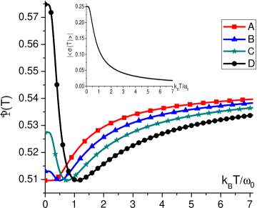
Figure 1: Change of the system purity ${\cal P}(T)$ with the bath temperature $T$. The values of the Euler angles $\theta_{a}^{(m)}$ are defined at the fixed temperatures $k_{B}T^{\star}/\omega_{0}=0$ (A), 0.5 (B), 0.75 (C) and 1.11 (D) due to the self-consistency condition (31) and are not changed after the measurement. The other Euler angles $\theta_{b}^{(1)}=4\pi/5$, $\Delta_{12}=7\pi/5$, $\Delta_{13}=3\pi/4$ are taken from the allowed “window” of values (A.26). In the inset: the temperature dependence of the initial coherence $|\langle\sigma(T)\rangle|\equiv|\langle\sigma_{\pm}(T)\rangle|$ at the parameters of the choice D.

It is seen that the purity minima are reached at temperatures $T^{\star}$ as it should be due to the self-consistency condition (31). However, both reduction and increase of the thermal bath temperature $T$ “pull” the system up from the most mixed state. A detailed analysis of the probabilities (IV) shows that in the zero-temperature limit the system purity is defined by the ground state amplitudes according to

$${\cal P}(T=0)=\sum\limits_{m=1}^{N}|C_{mn}|^{2}|a_{0}^{(m)}|^{2}|a_{0}^{(n)}|^{2},$$ (33)

whereas in the high-temperature limit the purity tends to the value

$${\cal P}(\beta\omega_{0}\ll 1)=\frac{1}{9}\,\sum\limits_{m=1}^{N}|C_{mn}|^{2}.$$ (34)

It is interesting that in this limit all the probabilities (IV) tend to $\omega_{m}=1/3$, which coincide with the extremal values $\omega_{m}^{(extr)}$ obtained in the case 1 at $\theta_{a}^{(m)}=\pi/2$. It can be concluded from Fig. 1 that at low values of $T^{\star}$ heating is favorable for the system purification while at high values of $T^{\star}$ cooling yields less mixed states. The highest considered value of $k_{B}T^{\star}/\omega_{0}=1.11$ corresponds to the maximal temperature, at which the self-consistency condition (31) still holds true at the chosen state vectors $|\varphi_{m}\rangle$, and the system is allowed to be at the global minimum of its purity. The general conclusion, which could be done after inspection of Fig. 1, consists in a remarkable fact that the system purity can be increased even by several tens of percents by temperature variation.

In the inset of Fig. 1, we depicted the temperature dependence of the initial system coherence $|\langle\sigma(T)\rangle|\equiv|\langle\sigma_{\pm}(T)\rangle|$ obtained at the parameters of the choice D. It is seen that the initial coherence follows the $\tanh(\beta\omega_{0}/2)$ rule and is never equal to zero.

Since the system-environment correlations play a constructive role at the early stage of the system evolution, and the coherence enhances at small times ourPRA , the initial state re-preparation by the temperature variation can be considered as an additional way to obtain a purer system. It should be stressed that it is possible to obtain a behavior of ${\cal P}(T)$ similar to that one presented in Fig. 1 even in the cases 1 and 2, but the minima of purity would be equal to 1/2. As we have already mentioned, no dynamic purification of the system could be possible in such a case.

We conclude this Section by consideration of some limiting cases, when the number of vectors in the subset $|\varphi_{m}\rangle$ is less than 3. At the same time, we allow the dimension of the vector subset $|\psi_{m}\rangle$ to be equal to $N=3$.

If $|\varphi_{m}\rangle\equiv|\varphi\rangle$ for any $m=\{1,2,3\}$, we obtain the pure state of the qubit after the nonselective measurement (see Eq. (IV)) since the probabilities $\omega_{m}$ are normalized to the unity. Here we are in a close resemblance with the measurement settings (62) of Ref. ourPRA , yielding the value (63) of the correlation contribution $\gamma_{cor}(t)$ to the generalized decoherence function $\tilde{\gamma}(t)$. In the Ohmic case MMR2012 , the system coherence starts to decrease monotonically from the value (65) to zero at $t\to\infty$.

At $|\varphi_{1}\rangle\neq|\varphi_{2}\rangle=|\varphi_{3}\rangle$, the situation is much more interesting. On the one hand, we have a mapping to the von Neumann-Lüders projection scheme ourPRA since

$$\varrho_{S}(0)=\omega_{1}|\varphi_{1}\rangle\langle\varphi_{1}|+\bar{\omega}_{2}|\varphi_{2}\rangle\langle\varphi_{2}|,\qquad\bar{\omega}_{2}=\omega_{2}+\omega_{3}.$$ (35)

To satisfy the condition (III) of the gradual coherence enhancement at small times, the measurement state vectors $|\varphi_{1}\rangle$ and $|\varphi_{2}\rangle$ have to be chosen to be orthonormal (see Eq. (55) of Ref. ourPRA ) or to obey Eqs. (66). However, no selections of the above mentioned state vectors can ensure the global minimum of the system purity, since the requirement $\omega_{1}^{(ext)}=\omega_{2}^{(ext)}=1/2$ (related to equalities $|a_{0}^{(1)}|^{2}=|a_{1}^{(1)}|^{2}=1/2$) contradicts the normalization conditions (7). Hence, at the case considered the system can be only in the state with a local minimum of purity, and we should not be afraid to obtain the completely decohered system after the measurement.

V The system response to the repeated nonselective measurements

In the previous section we discussed the influence of temperature variation on possible purification of the open quantum system. The temperature was supposed to have been changed right after the nonselective measurement.

Let us now consider a situation, when the system is subjected to the second nonselective measurement, which occurs immediately after the first one. We can also imagine a more general situation, when the system is subjected to the series of the repeated measurements at the initial instant of time $t=0$.

If such a measurement scheme is applied, the initial density matrix $\varrho^{\prime}_{SB}(0)$ of the composite system right after the first measurement obeys the equation

$$\varrho^{\prime}_{SB}(0)=\sum\limits_{m=1}^{N}\Omega^{\prime}_{m}\varrho_{SB}(0)\Omega^{\prime\dagger}_{m}.$$ (36)

This equation is analogous to the basic relation (1), where the equilibrium density matrix $\varrho_{eq}$ is replaced by the post-measurement one $\varrho_{SB}(0)$. The “primed” operators $\Omega^{\prime}_{m}$ are defined in the way similar to (6), where the state measurement vectors are replaced accordingly $|\varphi_{m}\rangle\rightarrow|\varphi^{\prime}_{m}\rangle$ and $|\psi_{m}\rangle\rightarrow|\psi^{\prime}_{m}\rangle$.

Thus, taking the trace in (36) over the bath variables, one can obtain the expression for the system density matrix $\varrho^{\prime}_{S}(0)$ after the second measurement,

$$\varrho^{\prime}_{S}(0)=\sum\limits_{n=1}^{N}\tilde{\omega}_{n}|\varphi^{\prime}_{n}\rangle\langle\varphi^{\prime}_{n}|,$$ (37)

where the probabilities $\tilde{\omega}_{n}$ after the second measurement are expressed

$$\tilde{\omega}_{n}=\sum\limits_{m=1}^{N}|D_{nm}|^{2}\omega_{m},\qquad D_{nm}=\langle\psi^{\prime}_{n}|\varphi_{m}\rangle$$ (38)

via the scalar products of the “old” $|\varphi_{m}\rangle$ and “new” (primed) $|\psi^{\prime}_{m}\rangle$ measurement state vectors.

The system purity right after the second measurement can be presented in the form similar to (27)

$${\cal P}^{\prime}=\sum\limits_{m,n=1}^{N}|C^{\prime}_{mn}|^{2}\tilde{\omega}_{m}\tilde{\omega}_{n},$$ (39)

where the matrix elements $C^{\prime}_{mn}$ are nothing but those of (26) defined on the “new” subset $|\varphi^{\prime}_{m}\rangle$.

It would be constructive to consider some different choices of the new measurement state vectors $|\psi^{\prime}_{m}\rangle$ and $|\varphi^{\prime}_{m}\rangle$ in relation to the change of the system purity.

V.1 Square root measurements

Suppose that the open quantum system after the first measurement was characterized by the density matrix (18). Now let us construct the “new” measurement state vectors $|\psi^{\prime}\rangle$ according the general rule

$$|\psi^{\prime}_{n}\rangle=\sqrt{\omega_{n}}\varrho_{S}^{-1/2}(0)|\varphi_{n}\rangle.$$ (40)

Here, $\varrho_{S}^{-1/2}(0)$ denotes the generalized inverse of the operator $\varrho_{S}^{1/2}(0)$. The operator $\varrho_{S}(0)$ as well as its square root are invertible since the rank $n$ of the density matrix $\varrho_{S}(0)$ is equal to the dimension of the Hilbert space ${\cal H}$ of the measurement state vectors. Moreover, its is a straightforward matter to calculate $\varrho^{-1/2}_{S}(0)$ explicitly for $2\times 2$ matrix of the initial density operator of the system.

The measurement state vectors $|\psi^{\prime}_{n}\rangle$, introduced by Eq. (40), are known to minimize SRM ; SRM1 the squared error $R$, determined by

$$R=\sum\limits_{n=1}^{N}\omega_{n}||\,|\varphi_{n}\rangle-|\psi^{\prime}_{n}\rangle||^{2}.$$ (41)

The definition (41) of the square error $R$ has to be considered in terms of the Hilbert-Schmidt norm of some specific operators constructed on the measurement state vectors $|\psi^{\prime}_{n}\rangle$ and $|\varphi_{n}\rangle$ (see Ref. SRM and the references herein for more details). Such schemes with the effects $F^{\prime}_{n}=|\psi^{\prime}_{n}\rangle\langle\psi^{\prime}_{n}|$, which realize the least-square root $R$, are known as the square root measurements (SRM) and are the subject of thorough investigation in the quantum measurement theory SRM ; SRM1 ; Holevo1979 .

Now let us look at the probabilities (38), when the basic subset of the measurement state vectors $|\psi^{\prime}_{m}\rangle$ is taken in the SRM form (40). It is obvious that

$$\tilde{\omega}_{n}=\sum\limits_{m=1}^{N}|\langle\varphi_{n}|\varrho_{S}^{-1/2}(0)|\varphi_{m}\rangle|^{2}\omega_{m}\omega_{n}$$ (42)

$$=\omega_{n}\large\langle\varphi_{n}|\varrho_{S}^{-1/2}(0)\underbrace{\!\sum\limits_{m=1}^{N}\omega_{m}|\varphi_{m}\large\rangle\large\langle\varphi_{m}|}_{\rho_{S}(0)}\varrho_{S}^{-1/2}(0)|\varphi_{n}\large\rangle\equiv\omega_{n}.$$

Thus, if one chooses $|\psi^{\prime}_{n}\rangle$ in the SRM form, then the system purity (39) after the second measurement is expressed via the probabilities $\omega_{n}$, obtained after the first measurement. Suppose that the system after the first measurement is prepared in the most mixed state; this minimal value of the purity is realized at $\omega_{n}^{(ext)}$ (see Eq.(29)), and the self-consistency condition (31) is obeyed. Now let us consider two possible selections of the subset $|\varphi^{\prime}_{m}\rangle$ of measurement state vectors:

1. The subsets of the the “new” and “old” vectors are different, $|\varphi^{\prime}_{m}\rangle\neq|\varphi_{m}\rangle$. After the second measurement, the extremum points $\tilde{\omega}^{(ext)}_{m}$ are shifted from their previous values, whereas the probabilities $\tilde{\omega}_{m}=\omega_{m}$ remain unchanged. Thus, the self-consistency condition (31) is now violated, and the system purity is no longer minimal;

2. The subsets of the “new” and “old” vectors are identical, $|\varphi^{\prime}_{m}\rangle\equiv|\varphi_{m}\rangle$. At this condition, “old” and “new” purities are the same since the state of the system does not change after the second measurement.

Hence, the result of the choice (40) of the “new” state vectors $|\psi^{\prime}_{m}\rangle$ can be ambiguous: in the case 1 we can assert that the system is not in the global minimum of purity after the second measurement, while in the case 2 the system remains in the same most mixed state, and the repeated measurement is useless from the viewpoint of the system purification.

V.2 Ordinary measurements

Now suppose that the definition (40) is not applied, and the measurement state vectors $|\psi^{\prime}_{m}\rangle$ are chosen to be arbitrary ones. Once again, let us suppose that the system was at the point of the global minimum of the purity after the first measurement and consider various choices of the subsets $|\varphi^{\prime}_{m}\rangle$:

1. The “new” and “old” subsets are identical, $|\varphi^{\prime}_{m}\rangle=|\varphi_{m}\rangle$. In such a case, the system purity is defined by Eq. (39), where the matrix elements are not changed, $C_{mn}=C^{\prime}_{mn}$. Contrary to the case 1 from the previous subsection, the extremum points $\omega_{m}^{(ext)}$ remain unaltered after the second measurement. However, the self-consistency condition (31) is violated since the system purity is determined by the “new” probabilities $\tilde{\omega}_{m}$ defined on the modified subset $|\psi^{\prime}_{m}\rangle\neq|\psi_{m}\rangle$. Thus, the system is no longer in the global minimum of purity after the second measurement;

2. Let us, in addition to the equality $|\varphi^{\prime}_{m}\rangle=|\varphi_{m}\rangle$, apply another condition, $|\psi^{\prime}_{m}\rangle=|\varphi_{m}\rangle$. The matrix elements $D_{mn}$, which define the “new” probabilities $\tilde{\omega}_{m}$ (see Eq. (38)), are now expressed as $D_{mn}=\langle\varphi_{m}|\varphi_{n}\rangle$. Suppose, we are performing the Neumann-Lüders projective measurements with $N=2$ and choose the vectors $|\varphi_{1}\rangle$ and $|\varphi_{2}\rangle$ to be orthogonal to each other (such a selection is one of the way to ensure the gradual growth of the system coherence at the initial stage of its evolution ourPRA ). At such a choice, the matrix elements transform into the Kronecker symbols, $D_{mn}=\delta_{mn}$. As a result, the “new” probabilities remain the same as the “old” ones, $\tilde{\omega}_{m}=\omega_{m}$. It means that nothing has been changed in the state of the system, and its purity is the same, ${\cal P^{\prime}}={\cal P}$.

   In all other cases (including the measurements on the overcomplete basis), $D_{mn}\neq\delta_{mn}$, thus $\tilde{\omega}_{m}$ $\neq$ $\omega_{m}$, and we actually come back to the item 1;

3. Now let us perform the second repeated measurement at the completely modified subsets $|\varphi^{\prime}_{n}\rangle\neq|\varphi_{n}\rangle$ and $|\psi^{\prime}_{n}\rangle\neq|\psi_{n}\rangle$. It is obvious that the extremum probabilities before and after the second measurement are different, $\tilde{\omega}^{(ext)}_{n}\neq\omega_{n}^{(ext)}$. To ensure that the system would not drop again into the global minimum of purity, it is necessary to violate the self-consistency condition (31). Using definitions (29) and (38)-(39), one can express this requirement as an inequality

   $$\frac{\sum\limits_{m,p=1}^{N}||\textbf{D}^{-1}||_{nm}||\textbf{ C}^{\prime-1}||_{mp}}{\sum\limits_{m,p=1}^{N}||\textbf{C}^{\prime-1}||_{mp}}\neq\frac{\sum\limits_{p=1}^{N}||\textbf{ C}^{-1}||_{nm}}{\sum\limits_{p,m=1}^{N}||\textbf{C}^{-1}||_{nm}},$$ (43)

   where $||\textbf{D}^{-1}||$ denotes the matrix inverse to $||\textbf{D}||\equiv|D_{mn}|^{2}$. The matrix $||\textbf{C}^{\prime}||$ is defined by (26) on the “new” (primed) subset of the measurement state vectors $|\varphi^{\prime}_{m}\rangle$.

   If condition (43) is satisfied, the system is not in the global minimum of its purity for sure. However, to clarify how pure the system is after the second measurement in comparison with its state after the first one, an additional study is necessary since the global minimum ${\cal P}_{min}$ can be higher than the non-extremal value ${\cal P}^{\prime}$.

To conclude this section, let us make a brief summary of the above considered cases from the viewpoint of a possible system purification:

• The measurement schemes discussed in the case 1, subsection A, as well as in the case 1, subsection B, are unambiguously promising since the system after the second measurement is pulled up from the global minimum of its purity. The same is true about the measurements on the overcomplete basis described in the case 2, subsection B;

• The scheme considered in the case 2, subsection A, is useless from this viewpoint since the system purity is not changed after the repeated measurement. The same is true about the special kind of the Neumann-Lüders projection scheme discussed in the case 2, subsection B;

• The case 3, subsection B, cannot give us unambiguous answer about the system purification and has to be studied in more details. However, at this measurement scheme the system is definitely not in the global minimum of its purity as compared with the first measurement.

VI Conclusions

In this paper, we study the initial state preparation of the qubit after the nonselective measurement, when the number of outcomes $N$ is greater than two. In such a scheme, the basis of the measurement state vectors is known to be overcomplete Holevo2001 ; SRM ; Holevo1979 , and the vectors are not orthonormal. To obtain the explicit results of practical importance, we have chosen the exactly solvable dephasing model Luczka ; MMR2012 and applied the conditions for the post-measurement state to ensure a gradual coherence enhancement ourPRA at the initial stage of the system evolution.

We show that at some special choices of parameters the system after the nonselective measurement can be prepared in the most mixed state. This case is strongly undesirable from the viewpoint of the quantum control measur since the system could remain in the completely decohered state, and no dynamic purification ourPRA of the qubit is possible. It is pointed out that, in general, the minimal value ${\cal P}_{min}$ of the system purity depends on the temperature of the thermal bath. Though at some measurement settings ${\cal P}_{min}$ can be equal to 1/2, and the system is totally decohered, there is still a possibility to purify the state of the qubit by changing temperature and, consequently, by making a re-distribution of populations of the levels.

We have also considered a more interesting case (from the practical viewpoint) when ${\cal P}_{min}>1/2$. At such measurement settings, both dynamical and temperature-controlled purifications are possible. We show that by altering the environment temperature after the nonselective measurement, it is possible to increase the system purity even by tens of percents. If the composite ($S+B$) system was initially prepared at low temperature, and the qubit was in the most mixed state, then heating is preferable. Otherwise, cooling yields a purer system.

However, there are also some other measurement settings, when the most mixed state of the system cannot be influenced by temperature, and the system purification is possible only after another measurement. In this case, a character of the minimum of ${\cal P}$ is very similar to that in the von Neumann-Lüders projection scheme, when the most mixed state of the qubit is always independent of temperature. We have listed the parameters options leading to such a scenario and noted that the measurement settings of this kind have to be avoided from the viewpoint of the problems of quantum control.

We have also considered two measurements, when the numbers of the state vectors in two basic subsets are different, and found out some similar and different features as compared to the case studied earlier ourPRA .

One of the ways to maintain the steady coherence of the system by a sequence of the repeated selective measurements due to the quantum Zeno effect is reported recently in Ref. Chaudhry14 . In our paper, we proceed in a bit different way and consider the sequence of the nonselective measurements performed instantly at the initial time $t=0$ of the system preparation. It turns out that some kinds of the measurement settings during such a repeated quantum measurements can be perspective from the viewpoint of an eventual system purification at $t=0$, while the other schemes do not allow to pull the system away from the point of global maximum of its mixedness. The action of some other schemes considered is ambiguous from the viewpoint of qubit purification, and it requires an additional study.

It would be interesting to verify our measurement schemes on more realistic systems, which allow not only the decoherence 27inPRA12 ; 28inPRA12 but also the population decay PRA2010 ; Ban ; severalW . However, it is a challenging problem because in this case the model can be no longer exactly solvable.

Appendix A Measurement settings that ensure condition (III)

To provide an enhancement of the system coherence, the Gram operator (8) in accordance with Eq. (III) has to be diagonal. Thus the following condition

$$\sum\limits_{m=1}^{3}\exp(i\phi_{b}^{(m)})\sin\theta_{b}^{(m)}=0$$ (A.1)

has to be ensured. Equating both the real and the imaginary parts of (A.1) to zero and expressing the third polar angle trough the remaining ones, it is possible to rewrite (A.1) as follows:

$$\sin\left(\phi_{b}^{(1)}-\phi_{b}^{(3)}\right)\sin\theta_{b}^{(1)}-\sin\left(\phi_{b}^{(2)}-\phi_{b}^{(3)}\right)\sin\theta_{b}^{(2)}=0,$$

$$\cos\phi_{b}^{(3)}\neq 0.$$ (A.2)

Now we consider three different options when condition (A) is satisfied.

A.1 The case $\sin\theta_{b}^{(1)}\neq 0$, $\sin\theta_{b}^{(2)}\neq 0$, $\phi_{b}^{(m)}-\phi_{b}^{(n)}=\pi k$.

These conditions assume that $\phi_{b}^{(1)}-\phi_{b}^{(3)}=\pi k$, $\phi_{b}^{(2)}-\phi_{b}^{(3)}=\pi l$, and $\phi_{b}^{(1)}-\phi_{b}^{(2)}=\pi(k-l)$, $\{k,l\}=\{0,1\}$. Having expressed two azimuthal angles via the third one and taking into account that

$$0\leq\theta_{b}^{(m)}\leq\pi,$$ (A.3)

one gets the following equations for $\theta_{b}^{(3)}$ (at the additional assumption $\theta_{b}^{(1)}>\theta_{b}^{(2)}$):

$$\sin\theta_{b}^{(3)}=\sin\theta_{b}^{(1)}-\sin\theta_{b}^{(2)}\quad\mbox{at}\quad k=1,\,l=0,$$

$$\sin\theta_{b}^{(3)}=\sin\theta_{b}^{(1)}+\sin\theta_{b}^{(2)}\quad\mbox{at}\quad k=l=1.$$ (A.4)

Eqs. (A.1) impose restrictions on the possible values of the polar angles $\theta_{b}^{(1)},\theta_{b}^{(2)}$ due to inequality (A.3).

The values (IV) in the case 1 can be expressed as

$$|C_{mn}|^{2}=\cos^{2}\frac{\left(\theta_{b}^{(m)}\mp\theta_{b}^{(n)}\right)}{2}.$$ (A.5)

The upper sign in Eq. (A.5) has to be taken for $\{m=1,n=2\}$ at $l=1$ and for $\{m=2,n=3\}$ at $l=0$; the lower sign has to be chosen for $\{m=1,n=3\}$ as well as for pairs $\{m=1,n=2\}$ at $l=0$ and $\{m=2,n=3\}$ at $l=1$.

In fact, in the case 1 we deal with a two-parameter problem at the nonselective measurement, where only two polar angles $\theta_{b}^{(1)}$ and $\theta_{b}^{(2)}$ are necessary. There is also a “window” of the allowed values for the third polar angle $\theta_{b}^{(3)}$ defined by Eqs. (A.3)-(A.1).

A.2 The case $\sin\theta_{b}^{(1)}\neq 0$, $\sin\theta_{b}^{(2)}=0$.

This case implies that $\theta_{b}^{(2)}=\pi k$, $k=\{0,1\}$, and $\phi_{b}^{(1)}-\phi_{b}^{(3)}=\pi$. Taking into account Eqs. (IV), (A.1) and having expressed $\theta_{b}^{(3)}$ via $\theta_{b}^{(1)}$, one can obtain after some algebra:

$$|C_{12}|^{2}=\cos^{2}(\theta_{b}^{(1)}/2),$$ (A.6)

$$|C_{13}|^{2}=\Biggl{[}\begin{array}[]{ccc}\cos^{2}\theta_{b}^{(1)}&\mbox{at}&\theta_{b}^{(3)}=\theta_{b}^{(1)},\\ 0&\mbox{at}&\qquad\theta_{b}^{(3)}=\pi-\theta_{b}^{(1)},\end{array}$$ (A.9)

$$|C_{23}|^{2}=\Biggl{[}\begin{array}[]{ccc}\cos^{2}(\theta_{b}^{(1)}/2)&\mbox{at}&\!\!\theta_{b}^{(3)}=\theta_{b}^{(1)},\\ \sin^{2}(\theta_{b}^{(1)}/2)&\mbox{at}&\quad\theta_{b}^{(3)}=\pi-\theta_{b}^{(1)}\end{array}$$ (A.12)

when $k=0$ or

$$|C_{12}|^{2}=\sin^{2}(\theta_{b}^{(1)}/2),$$ (A.13)

$$|C_{13}|^{2}=\Biggl{[}\begin{array}[]{ccc}\cos^{2}\theta_{b}^{(1)}&\mbox{at}&\theta_{b}^{(3)}=\theta_{b}^{(1)},\\ 0&\mbox{at}&\qquad\theta_{b}^{(3)}=\pi-\theta_{b}^{(1)},\end{array}$$ (A.16)

$$|C_{23}|^{2}=\Biggl{[}\begin{array}[]{ccc}\sin^{2}(\theta_{b}^{(1)}/2)&\mbox{at}&\!\!\!\theta_{b}^{(3)}=\theta_{b}^{(1)},\\ \cos^{2}(\theta_{b}^{(1)}/2)&\mbox{at}&\quad\theta_{b}^{(3)}=\pi-\theta_{b}^{(1)}\end{array}$$ (A.19)

when $k=1$.

It is seen that contrary to the case 1, this kind of the measurement settings needs only a single polar angle $\theta_{b}^{(1)}$.

A.3 The case $\sin\theta_{b}^{(1)}\neq 0$, $\sin\theta_{b}^{(2)}\neq 0$, $\phi_{b}^{(i)}-\phi_{b}^{(j)}\neq\pi k$.

Having denoted $\Delta_{ij}=\phi_{b}^{(i)}-\phi_{b}^{(j)}$, one can express $\theta_{b}^{(2)}$ and $\theta_{b}^{(3)}$ via the single polar angle $\theta_{b}^{(1)}$ as follows:

$$\sin\theta_{b}^{(2)}=\frac{\sin\Delta_{13}}{\sin(\Delta_{12}-\Delta_{13})}\sin\theta_{b}^{(1)},$$

$$\sin\theta_{b}^{(3)}=-\frac{\sin\Delta_{12}}{\sin(\Delta_{12}-\Delta_{13})}\sin\theta_{b}^{(1)}.$$ (A.20)

Taking into account the restriction (A.3), it is straightforward to verify that Eqs. (A.3) are satisfied at simultaneous realization of the following conditions:

$$\left\{\begin{array}[]{c}0<\Delta_{13}<\pi,\\ \pi<\Delta_{12}<2\pi,\\ 0<\Delta_{12}-\Delta_{13}<\pi,\\ \Delta_{13}+\arcsin[\sin\Delta_{13}\sin\theta_{b}^{(1)}]\leq\Delta_{12}\leq\pi+\Delta_{13}-\arcsin[\sin\Delta_{13}\sin\theta_{b}^{(1)}],\\ \Delta_{12}-\pi-\arcsin[\sin\Delta_{12}\sin\theta_{b}^{(1)}]\leq\Delta_{13}\leq\Delta_{12}+\arcsin[\sin\Delta_{12}\sin\theta_{b}^{(1)}].\end{array}\right.$$ (A.26)

It is seen from Eq. (A.3) that the case 3 implies the three-parameter measurement problem. However, like in the case 1, there exists a restriction on the possible values of the parameters $\Delta_{12}$, $\Delta_{23}$ and $\theta_{b}^{(1)}$ (see Eq.  (A.26) that, once again, yields a “window” for the allowed Euler angles.

Appendix B Measurement settings that ensure condition $\omega_{m}^{(ext)}=1/3$.

In the case 1 this condition is realized at $\theta_{a}^{(m)}=\pi/2$ and yields $|C_{12}|^{2}=|C_{13}|^{2}=|C_{23}|^{2}$. The last equality at $k=l=1$ due to (A.1)-(A.5) gives us the system of equations for three polar angles:

$$\left\{\begin{array}[]{c}\theta_{b}^{(1)}+\theta_{b}^{(2)}+2\theta_{b}^{(3)}=2\pi p,\\ 2\theta_{b}^{(1)}-\theta_{b}^{(2)}+\theta_{b}^{(3)}=2\pi q,\\ -\theta_{b}^{(1)}+2\theta_{b}^{(2)}+\theta_{b}^{(3)}=2\pi r,\end{array}\right.$$ (B.30)

where $\{p,q,r\}=\{0,1\}$. The system of equations (B.30) is compatible only at $r+q=p$. To satisfy this condition, we can choose $q=0$, $r=1$ and $p=1$ that yields

$$\theta_{b}^{(1)}=\frac{2\pi}{3}-\theta_{b}^{(3)},\,\,\theta_{b}^{(2)}=\frac{4\pi}{3}-\theta_{b}^{(3)},\,\,\frac{\pi}{3}<\theta_{b}^{(3)}<\frac{2\pi}{3}.$$ (B.31)

Another possible choice $q=1$, $r=0$, $p=1$ gives us a similar result:

$$\theta_{b}^{(1)}=\frac{4\pi}{3}-\theta_{b}^{(3)},\,\,\theta_{b}^{(2)}=\frac{2\pi}{3}-\theta_{b}^{(3)},\,\,\frac{\pi}{3}<\theta_{b}^{(3)}<\frac{2\pi}{3}.$$ (B.32)

If we select $l=0$, $k=1$, see Eqs. (A.1)-(A.5), we obtain the system of equations

$$\left\{\begin{array}[]{c}2\theta_{b}^{(1)}+\theta_{b}^{(2)}+\theta_{b}^{(3)}=2\pi p,\\ \theta_{b}^{(1)}+2\theta_{b}^{(2)}-\theta_{b}^{(3)}=2\pi q,\\ \theta_{b}^{(1)}-\theta_{b}^{(2)}+2\theta_{b}^{(3)}=2\pi r,\end{array}\right.$$ (B.36)

The system compatibility condition $r+q=p$ gives us two possible realizations:

$$\theta_{b}^{(1)}=\frac{4\pi}{3}-\theta_{b}^{(3)},\,\,\theta_{b}^{(2)}=-\frac{2\pi}{3}+\theta_{b}^{(3)},\,\,\frac{2\pi}{3}<\theta_{b}^{(3)}<\pi$$ (B.37)

at $q=0$, $r=1$, $p=1$, or

$$\theta_{b}^{(1)}=\frac{2\pi}{3}-\theta_{b}^{(3)},\,\,\theta_{b}^{(2)}=\frac{2\pi}{3}+\theta_{b}^{(3)},\,\,0<\theta_{b}^{(3)}<\frac{\pi}{3}$$ (B.38)

at $q=1$, $r=0$, $p=1$.

In the case 2 a simple analysis of Eqs. (A.6)-(A.13) shows that conditions $|C_{12}|^{2}=|C_{13}|^{2}=|C_{23}|^{2}$ leading to equation $\omega_{m}^{(ext)}=1/3$ are satisfied at

$$\theta_{b}^{(1)}=2\pi/3\qquad\mbox{if}\quad k=0,$$

$$\theta_{b}^{(1)}=\pi/3\qquad\,\,\,\mbox{if}\quad k=1.$$ (B.39)

The case $\theta_{b}^{(3)}=\pi-\theta_{b}^{(1)}$ has to be excluded from consideration since it gives $\omega_{m}^{(ext)}=\{1/2,0,1/2\}$. This result is unphysical (see Eq. (IV)) because we have postulated $a_{i}^{(m)}\neq 0$ for all the values of $m=\{1,2,3\}$.

A detailed analysis of the case 3 shows that the values (IV) can never be equal to each other (see also Eq. (A.3)). Hence, the condition $\omega_{m}^{(ext)}=1/3$ cannot be realized.

References

- (1) H.M. Wiseman, G.J. Milburn Quantum measurement and control (Cambridge University Press, Cambridge, 2009).
- (2) K. Saeedi, S. Simmons, J. Z. Salvail, P. Dluhy, H. Riemann, N. V. Abrosimov, P. Becker, H.-J. Pohl, J. J. L. Morton, and M. L. W. Thewalt, Science 342, 830 (2013).
- (3) A. Smirne, H.-P. Breuer, J. Piilo, and B. Vacchini, Phys. Rev. A 82, 062114 (2010).
- (4) V. Semin, I. Sinayskiy and F. Petruccione, Phys. Rev. A 86, 062114 (2012).
- (5) J. Dajka, B. Gardas, and J. Łuczka, Int. J. Theor. Phys. 52, 1148 (2012).
- (6) A. Z. Chaudhry and J. Gong, Phys. Rev. A 87, 012129 (2013).
- (7) V.G. Morozov, S. Mathey and G. Röpke, Phys. Rev. A 85, 022101 (2012).
- (8) A. Z. Chaudhry, and J. Gong, Phys. Rev. A 88, 052107 (2013).
- (9) V.V. Ignatyuk, V.G. Morozov, Phys. Rev. A 91, 052102 (2015)
- (10) H.-P. Breuer and F. Petruccione, The Theory of Open Quantum Systems (Oxford University, Oxford, 2002).
- (11) K. Kraus, States, Effects, and Operations, Lecture Notes in Physics, Vol. 190 (Springer, Berlin, 1983).
- (12) J. Werschnik, and E.K.U. Gross, J. Phys. B: At. Mol. Opt. Phys. 40, R175-R211 (2007).
- (13) V.B. Braginsky and F.Ya. Khalili, Quantum measurement (Cambridge University Press, Cambridge, 1992).
- (14) A.S. Holevo, Statistical structure of quantum theory, Lecture Notes in Physics, Monographs, M67, (Springer, Berlin, 2001).
- (15) S. Huang, Phys. Rev. A 72, 022324 (2005).
- (16) U. Hohenester, Optical Properties of Semiconductor Nanostructures: Decoherence Versus Quantum Control, in Handbook of Theoretical and Computational Nanotechnology edited by M. Rieth and W. Schommers (American Scientific Publishers, Valencia, 2006).
- (17) A. Montina and F.T. Arecchi, Phys. Rev. Lett. 100, 120401 (2008).
- (18) J. Łuczka, Phys. A (Amsterdam, Neth.) 167, 919 (1990).
- (19) A. Peres, Foundation of Physics 20, 1441 (1990).
- (20) W.G. Unruh, Phys. Rev. A 51, 992 (1995).
- (21) V.G. Morozov, G. Röpke, Condens. Matter Phys. 15, 43004 (2012).
- (22) V.V. Ignatyuk, V.G. Morozov, Condens. Matter Phys. 16, 34001 (2013).
- (23) P. Zanardi, D.A. Lidar, Phys. Rev. A 70, 012315 (2004).
- (24) Y.C. Eldar and G.D. Forney, IEEE Trans. Inf. Theory 47, 858 (2001).
- (25) A.S. Holevo, Theory Probab. Appl. 23, 411 (1979).
- (26) A. Z. Chaudhry and J. Gong, Phys. Rev. A 90, 012101 (2014).
- (27) D.I. Schuster et al., Nature (London) 445, 515 (2007).
- (28) A.D. Cronin, J. Schmiedmayer, and D.E. Pritchard, Rev. Mod. Phys. 81, 1051 (2009).
- (29) Masashi Ban, J. Mod. Optic. 58, 640 (2011).
- (30) R. Juárez-Amaro, A. Zúñiga-Segundo and H.M. Moya-Cessa, Appl. Math. Inf. Sci. 6, 1 (2014).