Tetraquark Production in Double Parton Scattering

Abstract

We develop a model to study tetraquark production in hadronic collisions. We focus on double parton scattering and formulate a version of the color evaporation model for the production of the $X(3872)$ and of the $T_{4c}$ tetraquark, a state composed by the $c\bar{c}c\bar{c}$ quarks. We find that the production cross section grows rapidly with the collision energy $\sqrt{s}$ and make predictions for the forthcoming higher energy data of the LHC.

I Introduction

I.1 Production mechanism

Over the last years the existence of exotic hadrons has been firmly established espo ; nnl and now the next step is to determine their structure. Among the proposed configurations the meson molecule and the tetraquark are the most often discussed. So far almost all the experimental information about these states comes from their production in B decays. The production of exotic particles in proton proton collisions is one of the most promising testing grounds for our ideas about the structure of the new states. It has been shown espo that it is extremely difficult to produce molecules in p p collisions. In the molecular approach the estimated cross section for $X(3872)$ production is two orders of magnitude smaller than the measured one. The present challenge for theorists is to show that these data can be explained by the tetraquark model. To the best of our knowledge, this has not been done so far. In this work we give a step in this direction, considering the production of the $X(3872)$ and of the $T_{4c}$, a state composed by two charm quark pairs: $c\bar{c}c\bar{c}$.

In recent high energy collisions at the LHC, it became relatively easy to produce 2psi7 ; 2psilhcb four charm quarks ($c\bar{c}c\bar{c}$) in the same event. Events with four heavy quarks can be treated as a particular case of $\alpha_{s}^{2}$ correction to the standard single gluon-gluon scattering, in which an extra $c\bar{c}$ pair is produced, i.e., the process $gg\rightarrow c\bar{c}c\bar{c}$. This is usually called single parton scattering (SPS). Another possible way to produce $c\bar{c}c\bar{c}$ is by two independent leading order gluon-gluon scatterings, i.e. two times the reaction $gg\rightarrow c\bar{c}$. This is usually called double parton scattering (DPS) dps1 ; dps2 . In fact, apart from $c\bar{c}c\bar{c}$, DPS events may generate many other different final states, such as four jets, a $c-\bar{c}$ pair plus two jets, etc. For our purposes, the other relevant DPS process is the production of a $c-\bar{c}$ pair plus a light quark pair, $q-\bar{q}$, which will hadronize and form the $X(3872)$. Since DPS events are in the realm of perturbative physics, the light quark pair must be produced with large invariant mass and the final state $X(3872)$ will carry large transverse momentum. This seems to be appropriate to describe the CMS data cms , where the $X(3872)$ was observed with a transverse momentum lying in the range $10\leq p_{T}\leq 25$ GeV. In nosdps ; anton it has been shown that DPS charm production is already comparable to SPS production at LHC energies. DPS grows faster with the energy because it is proportional to $g(x,\mu^{2})^{4}$ while SPS is proportional to $g(x,\mu^{2})^{2}$. Here $g(x,\mu^{2})$ is the gluon density in the proton as a function of the gluon fractional momentum $x$ and of the scale $\mu$ and it grows quickly with increasing collision energies. In the present work we shall consider the DPS events with the production of the two $c\bar{c}$ pairs and also with a $c\bar{c}$ and a light quark $q\bar{q}$ pair.

Once we have generated all the quarks and antiquarks needed to form the $X(3872)$ or the $T_{4c}$ in DPS events, we need to bind them together. To this end we shall use the main ideas of the Color Evaporation Model (CEM) cem ; ramona of charmonium production, where the $c-\bar{c}$ is “kinematically bound”, i.e., the charm pair sticks together because it does not have an invariant mass large enough to produce anything else. We shall use the CEM ideas to study $T_{4c}$ and $X(3872)$ production in DPS events. In the CEM formalism one parton from the hadron target scatters with one parton from the hadron projectile forming a charmonium state, which can absorb (emit) additional gluons from (to) the hadronic color field to become color neutral. This is the usual (SPS) $c\bar{c}$ production. At high energies the gluon density in the proton is much bigger than the sea quark density and hence, in what follows, we shall consider particle production only from gluon-gluon collisions. Now we are going to extend the CEM to the case where two gluons from the hadron target scatter independently with two gluons from the hadron projectile as depicted in Fig. 1, where we show DPS production of $T_{4c}$. In the figure two gluons collide and form a $c\bar{c}$ state with mass $M_{12}$, while other two gluons collide and form a second $c\bar{c}$ state with mass $M_{34}$. The two objects bind to each other forming the $T_{4c}$. Additional gluon exchanges with the environment are not shown in the figure. Replacing one $c\bar{c}$ pair by a light quark pair, $q\bar{q}$, the diagram would describe the production of $X(3872)$.

The main difference between a tetraquark and a meson molecule is that the former is compact and the interaction between the constituents occurs through color exchange forces whereas the latter is an extended object and the interaction between its constituents happens through meson exchange forces. In what was said above no explicit mention to size or color is made. However when we speak about the initial gluon fusion and about the final color neutralization through gluon emission or absorption it is understood that all this must happen within the confinement scale $\simeq 1$ fm. For this reason we believe that our model is suitable to describe tetraquark production. Although not explicitly excluded, it seems very unlikely that the clusters with masses $M_{12}$ and $M_{34}$ will form color singlets interacting through meson exchange.

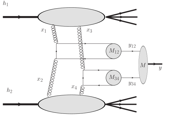
Figure 1: The gluons with odd (even) label come from the upper (lower) hadron, and carry momentum fraction $x_{i}$. The “gluon 1” scatters with “gluon 2”, making the state $M_{12}$. An analogous process occurs with gluons 3 and 4. Finally $M_{12}$ and $M_{34}$ merge and form the $T_{4c}$ with mass $M$.

I.2 Kinematics

Working with the usual CEM one-dimensional kinematics, the rapidities of the objects $M_{12}$ and $M_{34}$ are respectively:

$$y_{12}\,\,=\,\,\frac{1}{2}\ln\frac{x_{1}}{x_{2}}\,\,\,\,\,\,\,\,\mbox{and}\,\,\,\,\,\,\,\,y_{34}\,\,=\,\,\frac{1}{2}\ln\frac{x_{3}}{x_{4}}$$ (1)

and their invariant masses are

$$M_{12}=\sqrt{x_{1}\,x_{2}\,s}\,\,\,\,\,\,\,\,\mbox{and}\,\,\,\,\,\,\,\,M_{34}=\sqrt{x_{3}\,x_{4}\,s}\,\,.$$ (2)

In terms of these variables and in the low $p_{T}$ regime, the invariant mass of the $c\bar{c}c\bar{c}$ system is then given by:

$$M^{2}\,=\,M_{12}^{2}\,+\,M_{34}^{2}\,+\,2M_{12}\,M_{34}\,\cosh(y_{12}-y_{34})\,\,.$$ (3)

The $cosh$ function grows very rapidly with the argument and hence even a modest rapidity difference between the two clusters with $M_{12}$ and $M_{34}$ will significantly increase the value of $M$. We will then assume that both clusters move with equal rapidity, i.e. $y_{12}=y_{34}$, and become bound to each other, forming a system with mass:

$$M\,=\,M_{12}\,+\,M_{34}\,\,.$$ (4)

Finally, in order to produce the final tetraquark state with right mass, $M_{T}$, the cluster with mass $M$ emits or absorbs gluons carrying an energy $\Delta$, which will be discussed below. We have thus:

$$M\pm\Delta\,=\,M_{T}\,\,.$$ (5)

A remarkable difference between the standard CEM for charmonium production and the model developed here is in the role played by the limits of the integral over the squared invariant mass $M^{2}$. In the case of the usual $J/\psi$ production it goes from $(2m_{c})^{2}$ to $(2m_{D})^{2}$. This ensures that the $c-\bar{c}$ can never decay into open charm, not forming the charmonium state, because it does not have enough invariant mass. The case of the tetraquark $X(3872)$ is different. Suppose, for example, that we have the four-quark system with an invariant mass of $3740$ MeV. While this system can only form the $X$ resonance by absorbing some gluons (carrying energy $\Delta$) from the target or from the projectile, it has sufficient mass to decay immediately into a $D^{+}D^{-}$ pair and not form the resonance. Moreover, since the energy $\Delta$ is carried by an undefined number of gluons, this decay is not hindered by parity (or charge conjugation) conservation. Therefore, in our case, the integration over $M^{2}$ must be changed becoming more restrictive:

$$\int_{(2m_{c})^{2}}^{(2m_{D})^{2}}\,dM^{2}\,\,\rightarrow\,\,\int_{(M_{T}-\Delta)^{2}}^{(M_{T}+\Delta)^{2}}\,dM^{2}$$ (6)

where the left side refers to the usual CEM and the right side refers to tetraquark states. We will use this restriction in Sec. III.

II Tetraquark production

II.1 $T_{4c}$: the all-charm tetraquark

The $T_{4c}$ state was first discussed long time ago by Iwasaky iwasaky . In the eighties and early nineties, many authors ader1 ; ht ; brac ; sema addressed the subject arriving at different conclusions concerning the existence of a $c\bar{c}c\bar{c}$ bound state. More recently, with the revival of charmonium spectroscopy, Lloyd and Vary vary investigated the four-body $c\bar{c}c\bar{c}$ system obtaining several close-lying bound states. They found that deeply bound ($\simeq 100$ MeV) states may exist with masses around $6$ GeV. In Ref. javier the existence of $c\bar{c}c\bar{c}$ states was discussed in the framework of the hyperspherical harmonic formalism. The results suggested the possible existence of three four-quark bound states with quantum numbers $0^{+-}$, $2^{+-}$ and $2^{++}$ and masses of the order of $6.50$, $6.65$, and $6.22$ GeV. More recently, using the Bethe-Salpeter approach, the authors of Ref. heupel found an all-charm tetraquark with $J^{PC}=0^{++}$ and mass $M_{T_{4c}}=5.3\pm 0.5$ GeV. This mass is considerably lower than the $6.0$ GeV obtained in the previous model calculations iwasaky ; vary . It is also much lower than the $2\eta_{c}$ threshold. Potential decay channels into D mesons and pairs of light mesons necessarily involve internal gluon lines. The resulting decay width may therefore be rather small. On the other hand, preliminary lattice QCD calculations wagner ; bicudo seem to disfavor the existence of a deeply bound $c\bar{c}c\bar{c}$ state, being more compatible with a loosely bound $2\eta_{c}$ molecular state. In the works russo1 ; russo2 $T_{4c}$ production was studied in SPS events.

II.2 The production cross section

The cross section of the process shown in Fig. 1 can be calculated with the schematic DPS “pocket” formula:

$$\sigma_{DPS}\propto\frac{\sigma_{SPS}^{12}\sigma_{SPS}^{34}}{\sigma_{eff}}$$ (7)

where $\sigma_{eff}\simeq 15$ mb is a constant extracted from data analysis and $\sigma_{SPS}$ is the standard QCD parton model formula, i. e., the convolution of parton densities with partonic cross sections. To be more precise we expand the above formula showing the kinematical constraints introduced to study tetraquark production. It reads:

$$\sigma_{DPS} = \frac{F_{T_{4c}}}{\sigma_{eff}}\left[\int_{0}^{1}dx_{1}\int_{0}^{1}dx_{2}\,\,g(x_{1},\mu^{2})\,g(x_{2},\mu^{2})\,\sigma_{g_{1}g_{2}\to c\bar{c}}\right]$$ (8)

$$\times \,\,\left[\int_{0}^{1}dx_{3}\int_{0}^{1}dx_{4}\,\,g(x_{3},\mu^{2})\,g(x_{4},\mu^{2})\,\sigma_{g_{3}g_{4}\to c\bar{c}}\right]$$

$$\times \,\,\Theta(1-x_{1}-x_{3})\,\,\Theta(1-x_{2}-x_{4})\,\,\Theta(M_{12}^{2}-4m_{c}^{2})\,\,\Theta(M_{34}^{2}-4m_{c}^{2})$$

$$\times \,\,\delta(y_{34}-y_{12})$$

where $g(x,\mu^{2})$ is the gluon distribution in the proton with the gluon fractional momentum $x$ and at the factorization scale $\mu^{2}$ and $\sigma_{gg\to c\bar{c}}$ is the $gg\to c\bar{c}$ elementary cross-section. The step functions $\Theta(1-x_{1}-x_{3})$ and $\Theta(1-x_{2}-x_{4})$ enforce momentum conservation in the projectile and in the target. The step functions $\Theta(M_{12}^{2}-4m_{c}^{2})$ and $\Theta(M_{34}^{2}-4m_{c}^{2})$ guarantee that the invariant masses of the gluon pairs 12 and 34 are large enough to produce two charm quark pairs. The delta function implements the “binding condition” and $F_{T_{4c}}$ is a constant, analogous to the one appearing in the CEM formula, which represents the probability of the four-quark system to evolve to a particular tetraquark state.

In the above formula, all the variables depend on the momentum fractions $x_{1}$ … $x_{4}$. Because of the delta function, we know that the two clusters shown in Fig. 1 are “flying together” and that they form a system with mass $M=M_{12}+M_{34}$, which can take any value. In order to improve our kinematical description of this bound state, we can impose constraints on the values of $M$, such as (6). This can be best done rewritting (8) and changing variables from $x_{1}$, $x_{2}$, $x_{3}$ and $x_{4}$ to $y_{12}$, $y_{34}$, $M_{12}$ and $M_{34}$. We obtain:

$$\sigma_{DPS} = \frac{F_{T_{4c}}}{\sigma_{eff}}\left[\frac{1}{s}\int dy_{12}\int dM_{12}^{2}\,\,g(\bar{x_{1}},\mu^{2})\,g(\bar{x_{2}},\mu^{2})\,\sigma_{g_{1}g_{2}\to c\bar{c}}\right]$$ (9)

$$\times \,\,\left[\frac{1}{s}\int dy_{34}\int dM_{34}^{2}\,\,g(\bar{x_{3}},\mu^{2})\,g(\bar{x_{4}},\mu^{2})\,\sigma_{g_{3}g_{4}\to c\bar{c}}\right]$$

$$\times \,\,\Theta(1-\bar{x_{1}}-\bar{x_{3}})\,\,\Theta(1-\bar{x_{2}}-\bar{x_{4}})\,\,\Theta(M_{12}^{2}-4m_{c}^{2})\,\,\Theta(M_{34}^{2}-4m_{c}^{2})$$

$$\times \,\,\delta(y_{34}-y_{12})$$

where

$$\bar{x_{1}}=\frac{M_{12}}{\sqrt{s}}\,e^{y_{12}}\,\,\hskip 8.5359pt,\hskip 8.5359pt\bar{x_{2}}=\frac{M_{12}}{\sqrt{s}}\,e^{-y_{12}}\,\,\hskip 8.5359pt,\hskip 8.5359pt\bar{x_{3}}=\frac{M_{34}}{\sqrt{s}}\,e^{y_{34}}\,\,\hskip 8.5359pt,\hskip 8.5359pt\bar{x_{4}}=\frac{M_{34}}{\sqrt{s}}\,e^{-y_{34}}$$ (10)

and consequently

$$\Theta(1-\bar{x_{1}}-\bar{x_{3}})=\Theta(1-\frac{M_{12}}{\sqrt{s}}\,e^{y_{12}}-\frac{M_{34}}{\sqrt{s}}\,e^{y_{34}})\,\,\hskip 8.5359pt,\hskip 8.5359pt\,\,\Theta(1-\bar{x_{2}}-\bar{x_{4}})=\Theta(1-\frac{M_{12}}{\sqrt{s}}\,e^{-y_{12}}-\frac{M_{34}}{\sqrt{s}}\,e^{-y_{34}})$$ (11)

From the above expressions it is easy to see that when $y_{12}=y_{34}=y$, then (4) holds and the theta functions give lower and upper limits for the integration in $y$:

$$-\mbox{ln}\frac{\sqrt{s}}{M}\leq y\leq\mbox{ln}\frac{\sqrt{s}}{M}$$ (12)

The upper limit of $M_{12}$ and $M_{34}$ can be fixed imposing constraints on their sum, $M$. In the case of the $X(3872)$ we already know the mass of the state that we want to produce. In principle we could just use (4) with a fixed value of $M$. However, following the spirit of the CEM, we will assume that when the system with mass $M=M_{12}+M_{34}$ goes to the final state with mass $M_{T}$ it can absorb or emit soft gluons to neutralize color. These gluons carry an energy going from almost zero to the QCD scale, given by $\Delta=\mathcal{O}(\Lambda_{QCD})$. Then, from (4) and (5) we have:

$$M^{min}=M^{min}_{12}+M^{min}_{34}=M_{T}-\Delta$$ (13)

and

$$M^{max}=M^{max}_{12}+M^{max}_{34}=M_{T}+\Delta$$ (14)

From these equations we can see that, knowing the mass of the tetraquark state and fixing the amount of energy which can be exchanged in the formation of the final state, we constrain the limits in the integrations over $M_{12}$ and $M_{34}$. In the symmetric case of $T_{4c}$ production $M_{12}^{min}=M_{34}^{min}$, $M_{12}^{max}=M_{34}^{max}$, (13) and (14) completely fix these limits. In the case of the $X(3872)$, we may have different choices for $M_{12}^{min}(M_{12}^{max})$ and $M_{34}^{min}(M_{34}^{max})$ but they will be correlated.

III Numerical results and discussion

III.1 $T_{4c}$

As mentioned in the introduction we take the production cross section of the $T_{4c}$ as a baseline because it is heavy, and hence treatable in pQCD, and also to make some contact with the production of $c\bar{c}c\bar{c}$ in DPS. In this subsection we discuss the numerical results obtained for $T_{4c}$. Then in the following subsection, after only a few changes we calculate the cross section for $X(3872)$ production.

We now evaluate equation (9) replacing $g(x,\mu^{2})$ by the MRST gluon distribution mrst and $\sigma_{gg\rightarrow c\bar{c}}$ by the standard leading order QCD result ramona :

$$\sigma_{gg\rightarrow c\bar{c}}=\frac{\pi\alpha_{s}^{2}(m^{2})}{3m^{2}}\left\{{(1+\frac{4m^{2}_{c}}{m^{2}}+\frac{m^{4}_{c}}{m^{4}})\,ln[\frac{1+\beta}{1-\beta}]\,-\,\frac{1}{4}(7+\frac{31m^{2}_{c}}{m^{2}})\beta}\right\}$$ (15)

with

$$\beta=[1-\frac{4m^{2}_{c}}{m^{2}}]^{1/2}$$

where $m^{2}$ is equal to $M^{2}_{12}$ or $M^{2}_{34}$. A difficulty in our calculation is the uncertainty in the normalization of the cross section. Whereas in the case of charmonium production in the CEM we have experimental information, which can be used to fix the nonperturbative constant $F_{H}$, in the case of the $T_{4c}$ nothing is known. For the time being we can only try to make a simple estimate.

In the usual CEM it is assumed that the nonperturbative probability for the $Q\bar{Q}$ pair to evolve into a quarkonium state H is given by a constant $F_{H}$ that is energy-momentum and process independent. Once $F_{H}$ has been fixed by comparison with the measured total cross section for the production of the quarkonium H at one given energy, the CEM can predict, with no additional free parameters, the energy dependence of the production cross section and the momentum distribution of the produced quarkonium. Following the CEM strategy we shall adjust $\sigma_{T_{4c}}$ connecting it to the experimentally measured cross section of $X(3872)$ production at one single energy and then make predictions for higher energies.

We know that the production cross section of $T_{4c}$ must be smaller than the one for $X(3872)$ production and the latter has been measured by the CMS collaboration cms at $\sqrt{s}=7$ TeV. Moreover, assuming that the binding mechanism is the same, the only difference is that we must replace the light quark pair (which is in the $X(3872)$) by the $c\bar{c}$ pair, which is much more difficult to produce. Therefore, in order to estimate the cross section for producing the $T_{4c}$, we must multiply the $X(3872)$ production cross section, $\sigma_{X}$, by a penalty factor:

$$\sigma_{T_{4c}}=\frac{\sigma_{c\bar{c}c\bar{c}}}{\sigma_{c\bar{c}q\bar{q}}}\,\sigma_{X}\simeq\frac{\sigma_{c\bar{c}}\,\sigma_{c\bar{c}}}{\sigma_{c\bar{c}}\,\sigma_{q\bar{q}}}\,\sigma_{X}\simeq\frac{\sigma_{c\bar{c}}}{\sigma_{inel}}\simeq 0.12\,\sigma_{X}$$ (16)

where $\sigma_{c\bar{c}c\bar{c}}$ and $\sigma_{c\bar{c}q\bar{q}}$ are the cross sections for the production of $c\bar{c}c\bar{c}$ and $c\bar{c}q\bar{q}$ respectively. These cross sections can be measured in double parton scattering events. In the above expression, after using the factorization hypothesis, $\sigma_{c\bar{c}}$ cancels out and the ratio $\sigma_{c\bar{c}}/\sigma_{q\bar{q}}\simeq\sigma_{c\bar{c}}/\sigma_{inel}$ can be inferred from data siginel ; cc7 , which at $7$ TeV yield $\approx 0.12$. All the required numbers are collected in Table I. Finally, using the value of $\sigma_{X}\simeq 30$ nb cms , we have:

$$\sigma_{T_{4c}}(\sqrt{s}=7\,\mbox{TeV})\simeq(3.6\,\pm 2.5)\,\mbox{nb}$$ (17)

Having fixed the numbers we plot the cross section for $T_{4c}$ production as a function of the energy in Fig. 2. In order to obtain an estimate of the theoretical error we vary the parameters trying to scan the most relevant region in the parameter space. We choose $\Delta\approx\Lambda_{QCD}\approx 200$ MeV and we assume that the $T_{4c}$ mass is given by $M_{T_{4c}}=5.4$ GeV, as obtained in Ref. heupel . With these two parameters fixed we can choose different values for the charm mass $m_{c}$. However there is an upper limit for $m_{c}$, which cannot be bigger than $M_{12}^{min}/2$. Substituting $\Delta$ and $M_{T_{4c}}$ in Eq. (13) we find that $M_{12}^{min}=2.6$ GeV, consequently the maximum value for $m_{c}$ is $m_{c}=1.3$ GeV. In Fig. 2 the upper line corresponds to $m_{c}=1.2$ GeV and the lower line corresponds to $m_{c}=1.3$ GeV. The star in Fig. 2 corresponds to the central value at $\sqrt{s}=7$ TeV. Here the constant $F_{T_{4c}}$ was chosen so as to reproduce (17). Once all the parameters are fixed at $\sqrt{s}=7$ TeV, the energy dependence of the cross section is completely determined by the model. In Fig. 2 the cross represents the central value of our prediction for the energy $\sqrt{s}=14$ TeV:

$$\sigma_{T_{4c}}(\sqrt{s}=14\,\mbox{TeV})\simeq(7.0\,\pm 4.8)\,\mbox{nb}$$ (18)

The main feature of the curves is the rapid rise with $\sqrt{s}$, which might render the $T_{4c}$ observable already at 14 TeV. This same fast growing trend was observed in other estimates with DPS dps1 ; dps2 .

Table 1: $X(3872)$ and $T_{4c}$ production cross sections at $\sqrt{s}=7$ TeV and $\sqrt{s}=14$ TeV.

Energy (TeV)	$\sigma_{c\bar{c}}$ (mb)	$\sigma_{inel}$ (mb)	$\sigma_{X}$ (nb)	$\sigma_{T_{4c}}$ (nb)
7	8.5 cc7	73.2 siginel	30.0 cms	$3.6\,\pm\,2.5$
14			$44.6\,\pm\,17.7$	$7.0\,\pm\,4.8$

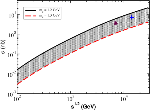
Figure 2: Cross section of $T_{4c}$ production as a function of the energy.

III.2 $X(3872)$

We now turn to the production cross section of $X(3872)$. We use the same parton densities as in the previous subsection and also the elementary cross section for heavy quark production (15). Note that we use this expression even for light quark production $\sigma_{g_{3}g_{4}\to q\bar{q}}$, which appears now in the second line of (8) or (9). Since this expression only holds for heavy enough quarks, its use here is questionable. In spite of this uncertainty, the existing experience in the literature is encouraging. In guti the authors used (15) to compute the cross section of strange particle production and calculated the asymmetries in the production of $K^{+}/K^{-}$, $\Lambda/\bar{\Lambda}$, …etc. They have used the convolution formula of the parton model and have taken the strange quark mass to be $m_{s}\simeq 500$ MeV. They could reproduce well the existing data on asymmetries. In our case the invariant mass $M_{34}$ defines the perturbative QCD scale and hence we must have $M_{34}>1$ GeV. This can be achieved with the light quarks having masses close to zero and transverse momenta in the few GeV region. Since we are using the one-dimensional version of the CEM, instead of transverse momentum we will assign an effective mass to the light quarks, $m_{q}=0.5$ GeV, which garantees that $M_{34}>2m_{q}>1$ GeV. Moreover, choosing $N_{f}=2$ and $\Lambda_{QCD}=200$ MeV, we have typically:

$$\alpha_{s}=\frac{12\pi}{(33-2N_{f})\,\mbox{ln}(\frac{(2m_{q})^{2}}{\Lambda_{QCD}^{2}})}\simeq 0.4$$ (19)

Although we may expect significant corrections, this number is still small enough for perturbation theory to make sense. As in the previous subsection, after fixing these parameters and knowing the tetraquark mass $M_{X}=3872$ MeV the only remaining free parameters are the charm mass and the constant $F_{X}$. We show our results in Fig. 3, where the upper line corresponds to $m_{c}=1.2$ GeV and the lower line corresponds to $m_{c}=1.3$ GeV. The constant $F_{X}$ was adjusted so that the central value of the cross section at $\sqrt{s}=7$ TeV (shown with a star) corresponds to $\sigma_{X}=30.0$ nb. With all the numbers fixed at the lower energy the energy dependence is given by the model. At $\sqrt{s}=14$ TeV, the cross indicates the central value of our prediction:

$$\sigma_{X}(\sqrt{s}=14\,\mbox{TeV})\simeq 44.6\,\pm 17.7\,\mbox{nb}$$ (20)

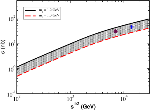
Figure 3: $X(3872)$ production cross section as a function of the energy.

The error in the number given above is relatively large but, at least we can predicit the order of magnitude of the cross section. As a first estimate with DPS, we think that the result is satisfactory. The model presented here can be improved in several aspects. Probably the most relevant one is the prescription to form the resonance, i.e., the hadronization of the multiquark system. Progress in this direction would also benefit the SPS calculations of this process. Our prescription, based mostly on the kinematical aspects and using only the rapidities and invariant masses, is not accurate enough and is the largest source of uncertainties. Work along this line is in progress. The other sources of uncertainties are, as usual, the choice of parton densities, the choice of the energy scale at which they are computed, the choice of the scale at which $\alpha_{s}$ is computed, the choice of $\Lambda_{QCD}$, and the charm and light quark masses.

IV Conclusion

We have developed a model for tetraquark production which combines double parton scattering and the basic ideas of the color evaporation model. We have made predictions for the $X(3872)$ production cross section, which may be confronted with the forthcoming LHC data taken at $\sqrt{s}=14$ TeV.

The results presented above contain some uncertainties: i) they do not include tetraquark production in SPS events, which can be larger than the DPS cross section. The calculation of the SPS cross section requires some fragmentation function which is not known.; ii) the binding mechanism is probably too simple and insensitive to the quantum numbers of the involved particles; iii) in the case of $X(3872)$ production, the use of formula (15) for light quark production is questionable. This problem may be circunvented using the next-to-leading order version of the CEM, in which the transverse momentum is included. In this case the light quarks can be really light but they have large $p_{T}$, rendering plausible the use of the perturbative formula (15).

References

References

- (1) A. Esposito, A. L. Guerrieri, F. Piccinini, A. Pilloni and A. D. Polosa, Int. J. Mod. Phys. A 30, 1530002 (2014).
- (2) M. Nielsen and F. S. Navarra, Mod. Phys. Lett. A 29, 1430005 (2014); M. Nielsen, F. S. Navarra and S. H. Lee, Phys. Rept. 497, 41 (2010); F. S. Navarra, M. Nielsen and S. H. Lee, Phys. Lett. B 649, 166 (2007).
- (3) V. Khachatryan et al. [CMS Collaboration], JHEP 1409, 094 (2014).
- (4) R. Aaij et al. [LHCb Collaboration], Phys. Lett. B 707, 52 (2012).
- (5) R. Astalos et al., “Proceedings of the Sixth International Workshop on Multiple Partonic Interactions at the Large Hadron Collider,” arXiv:1506.05829 [hep-ph]; M. Diehl, PoS DIS 2013, 006 (2013); [arXiv:1306.6059 [hep-ph]].
- (6) For recent reviews see S. Bansal et al., arXiv:1410.6664 [hep-ph]; A. Szczurek, Acta Phys. Polon. Supp. 8, 483 (2015); Acta Phys. Polon. B 46, 1415 (2015).
- (7) S. Chatrchyan et al. [CMS Collaboration] , JHEP 1304, 154 (2013).
- (8) E. R. Cazaroto, V. P. Goncalves and F. S. Navarra, Phys. Rev. D 88, 034005 (2013).
- (9) M. Luszczak, R. Maciula and A. Szczurek, Phys. Rev. D 85, 094034 (2012).
- (10) See N. Brambilla et al., Eur. Phys. J. C 71, 1534 (2011) and references therein.
- (11) R. Vogt, Ultrarelativistic Heavy Ion Colisions, Elsevier (2007), pg. 396.
- (12) Y. Iwasaki, Prog. Theor. Phys. 54, 492 (1975).
- (13) J.P. Ader, J.-M. Richard, and P. Taxil, Phys. Rev. D 25, 2370 (1982); J.L. Ballot and J.-M. Richard, Phys. Lett. B 123, 449 (1983); H.J. Lipkin, Phys. Lett. B 172, 242 (1986).
- (14) L. Heller and J.A. Tjon, Phys. Rev. D 32, 755 (1985); ibid 35, 969 (1987).
- (15) B. Silvestre-Brac, Phys. Rev. D 46, 2179 (1992).
- (16) B. Silvestre-Brac and C. Semay, Z. Phys. C 57, 273 (1993); ibid 5̱9, 457 (1993); ibid 61, 271 (1994).
- (17) R. J. Lloyd and J. P. Vary, Phys. Rev. D 70, 014009 (2004).
- (18) N. Barnea, J. Vijande and A. Valcarce, Phys. Rev. D 73, 054004 (2006).
- (19) W. Heupel, G. Eichmann and C. S. Fischer, Phys. Lett. B 718, 545 (2012).
- (20) M. Wagner, A. Abdel-Rehim, C. Alexandrou, M. Dalla Brida, M. Gravina, G. Koutsou, L. Scorzato and C. Urbach, J. Phys. Conf. Ser. 503, 012031 (2014).
- (21) P. Bicudo, K. Cichy, A. Peters, B. Wagenbach and M. Wagner, Phys. Rev. D 92, 014507 (2015).
- (22) A. V. Berezhnoy, A. K. Likhoded, A. V. Luchinsky and A. A. Novoselov, Phys. Rev. D 84, 094023 (2011).
- (23) A. V. Berezhnoy, A. V. Luchinsky and A. A. Novoselov, Phys. Rev. D 86, 034004 (2012).
- (24) A. D. Martin, R. G. Roberts, W. J. Stirling and R. S. Thorne, Eur. Phys. J. C 4, 463 (1998).
- (25) B. Abelev et al. [ALICE Collaboration], Eur. Phys. J. C 73, 2456 (2013).
- (26) B. Abelev et al. [ALICE Collaboration], JHEP 1207, 191 (2012).
- (27) T. D. Gutierrez and R. Vogt, Nucl. Phys. A 705, 396 (2002).