Distributed Event-based State Estimation

Abstract

An event-based state estimation approach for reducing communication in a networked control system is proposed. Multiple distributed sensor-actuator-agents observe a dynamic process and sporadically exchange their measurements and inputs over a bus network. Based on these data, each agent estimates the full state of the dynamic system, which may exhibit arbitrary inter-agent couplings. Local event-based protocols ensure that data is transmitted only when necessary to meet a desired estimation accuracy. This event-based scheme is shown to mimic a centralized Luenberger observer design up to guaranteed bounds, and stability is proven in the sense of bounded estimation errors for bounded disturbances. The stability result extends to the distributed control system that results when the local state estimates are used for distributed feedback control. Simulation results highlight the benefit of the event-based approach over classical periodic ones in reducing communication requirements.

1 Introduction

In almost all control systems today, data is processed and transferred between the system’s components periodically. While periodic system design is often convenient and well understood (Åström and Wittenmark, 1997), it involves an inherent limitation: data is processed and transmitted at predetermined time instants, irrespective of the current state of the system or the information content of the data. That is, system resources are used regardless of whether there is any need for processing and communication or not. This becomes prohibitive when resources are scarce, such as in networked or cyber-physical systems (Hespanha et al., 2007; Kim and Kumar, 2012) where multiple controllers share a communication medium, or wireless sensor networks (Akyildiz et al., 2002) where communication is typically a main consumer of battery power.

Because of the limitations of traditional design methodologies for resource-constrained problems, aperiodic or event-based strategies have recently received a lot of attention in the controls community (see e.g. Lemmon (2010); Heemels et al. (2012); Grüne et al. (2014); Cassandras (2014)), as well as related disciplines (Delbrück et al. (2010) and Tsividis (2010), for example). With event-based methods, data is transmitted or processed only when certain events indicate that an update is required, for example, to meet some control or estimation specification. Thus, resources are used only when required and saved otherwise.

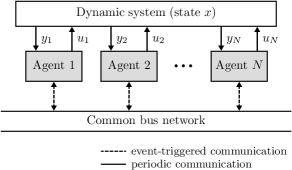
Figure 1: Networked control system. Multiple distributed agents make observations $y_{i}$ of a dynamic system and apply control actions $u_{i}$. The agents communicate via a common bus. The development of an event-based scheme for reducing inter-agent communication is the object of this report.

In this report, we propose a novel event-based scheme for distributed state estimation. We consider the networked control system (NCS) shown in Fig. 1, where multiple sensor-actuator-agents observe and control a dynamic system, and exchange data with each other over a common bus. Each agent shall estimate the full state of the dynamic system from its local sensors and data received over the bus. Because no local observability is assumed, agents rely on the inter-agent communication to solve the estimation problem. However, in order to limit network traffic, local event triggers on each agent ensure that updates are sent only when needed. The local state estimates can be used for feedback control to compute commands to the local actuators.

While the method can thus be used both for distributed event-based state estimation and control, the primary focus herein is on the state estimation problem. Since the developed event-based protocols for measurement and input communication serve the purpose of obtaining bounded state estimates, we refer to this method as event-based state estimation. The proposed method is distributed in the sense that data from distributed sensors is required for stable state estimation, and that transmit decisions are made locally on each agent.

The common bus (cf. Fig. 1) is a key component of the developed event-based approach. When one agent transmits sensor and input data, these can be received by all other agents. This will allows the agents to compute consistent estimates and use these for the triggering decisions (while inconsistencies can still happen due to data loss or delay). Wired fieldbus systems, which support broadcast communication between multiple devices, are common in industry (Thomesse, 2005). Recently, Ferrari et al. (2012) have shown that common bus concepts are feasible even for low-power wireless networks.

The approach for distributed event-based estimation proposed herein mimics a classic centralized, periodic, linear state observer design. The gains of the distributed state observers are simply taken from the centralized design. In each step, the appropriate subset of gains is chosen corresponding to which measurements have been received. The main focus of this report is to prove stability of the resulting switching and distributed estimation scheme. Challenges are 1) the switching nature of the observers (Böker and Lunze, 2002), and 2) the distributed arrangement of estimators coupled through the dynamics and the inter-agent communication. The stability results for state estimation extend in a straightforward manner to the control system resulting when local estimates are used for feedback. Beyond stability of the centralized design, no other assumptions are required.

Preliminary results of those herein were presented in the conference papers (Trimpe, 2012, 2014). Compared to these, the framework is extended herein to also include event-based communication of control inputs, which further reduces network traffic. In addition, we streamlined the presentation, significantly expanded review of related work, and added new simulation examples.

1.1 Related work

Early work on event-based state estimation concerned problems with a single sensor and estimator node, e.g. a sensor transmitting local state estimates to a remote estimator. Imer and Basar (2005) and Rabi et al. (2006) seek optimal sending rules for finite-horizon problems when the sensor has a fixed number of allowed transmissions, while Xu and Hespanha (2004) consider infinite-horizon problems. Typically, the optimal sending strategies are found to be policies with time-varying thresholds for finite-horizon problem, and constant thresholds for infinite-horizon problems, (Lemmon, 2010, p. 340). Because we are primarily interested in long-term behavior (stability) in this work, and also for simplicity of implementation, we consider constant thresholds.

Different types of stationary triggering policies have been suggested in literature. With the send-on-delta (SoD) protocol (Miskowicz, 2006), transmissions are triggered based on the difference of the current and last-transmitted measurement. While SoD and variations thereof can be considered as general-purpose triggers, a number of triggering mechanisms have been tailored to the state estimation problem. Measurement-based triggering (Trimpe and D’Andrea, 2011a) or predicted sampling (Sijs et al., 2014) places a threshold on the measurement innovation; that is, the difference of the current measurement and its prediction based on a process model. Thus, this trigger captures a quantity directly relevant for the state estimation. Wu et al. (2013) use the same trigger, but apply a transformation to decorrelate the innovation. Considering the variance of the innovation instead yields variance-based triggering (Trimpe and D’Andrea, 2011b, 2014). Marck and Sijs (2010) proposed relevant sampling, where the relative entropy of prior and posterior state distribution is employed as a measure of information gain. While all these triggers are deterministic, Han et al. (2015) have suggested a stochastic trigger, which maintains a Gaussian innovation process and thus facilitates theoretical analysis. In this work, we use measurement-based triggers, which are straightforward to implement and effective for event-based estimation (see comparisons by Sijs et al. (2014); Trimpe and Campi (2015)).

Besides the event trigger, the second main component of an event-based estimation method is the estimation or filtering algorithm. In the context of event-based estimation, a particular focus is on how the information contained in non-events, i.e. instants when no data is transmitted, is handled. For example, not receiving an update with SoD means that the current measurement is within a range of the last transmitted one. Taking a probabilistic viewpoint, it is clear how to fuse this information: the Bayesian estimator simply conditions on the available information, whether it is a data point or a set. However, this typically yields a non-Gaussian posterior and intractable algorithms. Therefore, different approximations have been suggested in literature (Henningsson and Åström, 2006; Sijs and Lazar, 2012; Sijs et al., 2013). If one ignores the extra information from non-events in favor of a standard implementation, a time-varying Kalman filter (KF) can be used (Trimpe and D’Andrea (2011a), for example). Herein, we use the same linear estimator structure as for the standard KF, but with constant, switching gains taken from a centralized design. The approach thus has the lowest computational complexity of all mentioned algorithms.

Most of the above works focus on single-link estimation problems. To the best of the author’s knowledge, distributed event-based state estimation with multiple sensor and estimator nodes, and dynamic couplings was first studied by Trimpe and D’Andrea (2011a). Considering the same architecture as in Fig. 1, each agent implements KFs as estimators and measurement-based triggers for transmit decisions. While Yook et al. (2002) had proposed the use of state estimators for the purpose of saving communication before, they do not employ state estimation in the usual sense. Instead of fusing model-based predictions with incoming data, they reset parts of the state vector. Later results on distributed event-based estimation for related, but different scenarios to the one herein, include the work by Weimer et al. (2012); Battistelli et al. (2012); Shi et al. (2014). These works consider a central fusion node, while estimation is distributed herein. Yan et al. (2014); Liu et al. (2015) treat problems where estimation is distributed over several nodes communicating according to a graph topology. However, these works employ simpler SoD-type triggers, which do not take advantage of model-based predictions for making more effective transmit decisions (see (Trimpe and Campi, 2015)). None of the mentioned references treats the problem of emulating a given centralized observer design with a distributed and event-triggered implementation, which does not rely on any assumptions except stability of the centralized design.

When the event-based state estimators are connected to state-feedback controllers, this structure represents a distributed event-based output-feedback control system. Wang and Lemmon (2008, 2011) and Mazo Jr and Tabuada (2008, 2011) were among the first to discuss distributed or decentralized implementations of event-based control for physically coupled systems. Whereas Wang and Lemmon assume weakly coupled dynamic systems, Mazo Jr and Tabuada have no assumption on the system coupling, yet rely on a centralized controller. While we use distributed control computations and distributed event triggering without any assumption on the system couplings, we rely on a common bus network. In contrast to the mentioned works, which assume perfect state information, we deal with noisy output measurements. Other results on distributed or decentralized event-based control for different scenarios include (Donkers and Heemels, 2012; Dimarogonas et al., 2012; Stöcker et al., 2013; Persis et al., 2013; Molin and Hirche, 2014; Tallapragada and Chopra, 2014; Sigurani et al., 2015), for example.

The key ideas of the approach to event-based estimation taken herein are conceptually related to the approach for event-based control by Lunze and Lehmann (2010). Therein, the authors design an event triggering scheme such that the difference between the state of a reference system with continuous feedback and the state of the event-based design is bounded. Here, a centralized Luenberger observer serves as the reference estimator, and event triggers are designed such that the event-based implementation mimics the reference design.

1.2 Notation

$\mathbb{R}$, $\mathbb{N}$, and $\mathbb{N}_{N}$ denote real numbers, positive integers, and the set $\{1,2,\dots,N\}$, respectively. Where convenient, vectors are expressed as tuples $(v_{1},v_{2},\dots)$, where $v_{i}$ may be vectors themselves, with dimension and stacking clear from context. For $v\in\mathbb{R}^{n}$ and $q\in[1,\infty]$, $\|v\|_{q}$ (or simply $\|v\|$) denotes the vector Hölder norm $\|v\|_{q}=(\sum\nolimits_{j=1}^{n}|v_{j}|^{q})^{1/q}$ for $1\leq q<\infty$, and $\|v\|_{q}=\max_{j\in\{1,\dots,n\}}|v_{j}|$ for $q=\infty$, (Bernstein, 2005). For a matrix $A$, $\|A\|_{q}$ (or simply $\|A\|$) denotes the matrix norm of $A$ induced by the chosen vector norm. For a time-indexed sequence $v=\{v(0),v(1),v(2),\dots\}$, $\|v\|_{\infty}$ denotes the $\ell^{\infty}$ norm $\|v\|_{\infty}:=\sup\nolimits_{k\geq 0}\,\|v(k)\|$, (Callier and Desoer, 1991). We use $\operatorname*{avg}_{i=1,\dots,N}(v_{i}):=\frac{1}{N}\sum\nolimits_{i=1}^{N}v_{i}$ to denote the average of $v_{1},\dots,v_{N}$ and omit the index “$i=1,\dots,N$” when clear from context. For an estimate of $x(k)$ computed from measurement data until time $\ell\leq k$, we write $\hat{x}(k|\ell)$. For ease of notation, we also write $\hat{x}(k)$ for $\hat{x}(k|k)$. Finally, a matrix is called stable if all its eigenvalues have magnitude strictly less than one.

2 Preliminaries and Problem Formulation

In this section, we formally introduce the considered NCS and the centralized observer-based control design, which serves as a reference for the distributed and event-based scheme developed in this report.

2.1 Networked control system

We consider the NCS in Fig. 1 with $N$ sensor-actuator-agents. The dynamics of the entire system are described by the discrete-time, linear, time-invariant system

$$x(k) =Ax(k-1)+Bu(k-1)+v(k-1)$$ (1)

$$y(k) =Cx(k)+w(k)$$ (2)

with time index $k\in\mathbb{N}$ (corresponding to a sampling time $T_{s}$), state $x(k)\in\mathbb{R}^{n}$, control input $u(k)\in\mathbb{R}^{q}$, measurement $y(k)\in\mathbb{R}^{p}$, disturbances $v(k)\in\mathbb{R}^{n}$, $w(k)\in\mathbb{R}^{p}$, and all matrices of corresponding dimensions. We assume that $(A,B)$ is stabilizable and $(A,C)$ is detectable. No specific assumptions on the characteristics of the disturbances $v(k)$ and $w(k)$ are made; they can be random variables or deterministic disturbances. Most results herein apply to both scenarios.

The vectors $u(k)$ and $y(k)$ represent the collective inputs and measurements of the $N$ agents. We use $y_{i}(k)\in\mathbb{R}^{p_{i}}$ and $u_{i}(k)\in\mathbb{R}^{q_{i}}$ to denote the individual measurements and inputs by agent $i\in\mathbb{N}_{N}$; that is, $u(k)=(u_{1}(k),$ $u_{2}(k),$ $\dots,$ $u_{N}(k))$ and $y(k)=(y_{1}(k),y_{2}(k),\dots,y_{N}(k))$. With this, (1) and (2) can be rewritten as

$$x(k) =Ax(k-1)+\sum_{i\in\mathbb{N}_{N}}B_{i}u_{i}(k-1)+v(k-1)$$ (3)

$$y_{i}(k) =C_{i}x(k)+w_{i}(k)\qquad\forall\,i\in\mathbb{N}_{N}$$ (4)

where the dimensions of $B_{i}$, $C_{i}$, and $w_{i}$ follow from $y_{i}$ and $u_{i}$. Agents can be heterogeneous with different types and dimensions of measurements and inputs, including the possibility of no sensors ($p_{i}=0$) or actuators ($q_{i}=0$). To avoid special treatment of this case in the following, a summation involving a signal of zero dimension (such as (3) for some $q_{i}=0$) is understood to not include the corresponding summand. We do not make any assumption on stabilizability and detectability for the individual agents; that is, $(A,B_{i})$ can possibly be not stabilizable, and $(A,C_{i})$ not detectable.

The agents are connected over a common-bus network as shown in Fig. 1, over which they can exchange measurements and inputs. Supported by the bus, all agents will receive the data if one agent communicates. Agents are assumed to be synchronized in time, and network communication is abstracted as instantaneous.

2.2 Centralized design with periodic communication

For stabilizing (1), (2), a centralized control system, which has periodic access to all measurements $y$ and computes all inputs $u$, can readily be designed as the combination of a state estimator and a state-feedback law. A linear, time-invariant state estimator is given by

$$\hat{x}_{\text{c}}(k|k-1)=A\hat{x}_{\text{c}}(k-1|k-1)+Bu(k-1)$$ (5)

$$\hat{x}_{\text{c}}(k|k)=\hat{x}_{\text{c}}(k|k-1)+L\big{(}y(k)-C\,\hat{x}_{\text{c}}(k|k-1)\big{)}$$ (6)

with static estimator gain $L$. For the later development, we rewrite (6) as

$$\hat{x}_{\text{c}}(k|k) =\hat{x}_{\text{c}}(k|k-1)+\!\!\sum_{\ell\in\mathbb{N}_{N}}\!L_{\ell}\big{(}y_{\ell}(k)-C_{\ell}\hat{x}_{\text{c}}(k|k-1)\big{)}$$

$$\text{with}\quad L=[L_{1},L_{2},\dots,L_{N}],\,L_{i}\in\mathbb{R}^{n\times p_{i}}.$$ (7)

We further consider the static state-feedback controller

$$u(k)=F\hat{x}_{\text{c}}(k)$$ (8)

with controller gain $F$ (recall that $\hat{x}_{\text{c}}(k)=\hat{x}_{\text{c}}(k|k)$). The centralized closed-loop control system (1), (2), (5), (6), and (8) is described by

$$x(k) =(A\!+\!BF)x(k\!-\!1)-BF\epsilon_{\text{c}}(k\!-\!1)+v(k\!-\!1)$$ (9)

$$\epsilon_{\text{c}}(k) =(I\!-\!LC)A\epsilon_{\text{c}}(k\!-\!1)+(I\!-\!LC)v(k\!-\!1)-Lw(k)$$ (10)

where $\epsilon_{\text{c}}(k)=x(k)-\hat{x}_{\text{c}}(k)$ is the centralized estimation error. A standard result and obvious from (9), (10), the closed-loop system is stable if both estimation error and state dynamics are stable, which we shall assume:

Assumption 1.

$L$ is such that $(I-LC)A$ is stable.

Assumption 2.

$F$ is such that $A+BF$ is stable.

Because $(A,B)$ is stabilizable and $(A,C)$ detectable, such gains exist and can be computed using standard methods (see e.g. (Åström and Wittenmark, 1997)).

2.3 Problem statement

We seek a distributed and event-based state estimation design that emulates the centralized estimator (5) and (6) up to guaranteed bounds and with lower average communication requirements. Furthermore, the stability results for estimation shall be extended to the distributed event-based control system that is obtained when the state estimates are used for state-feedback control (8). State estimators, controllers, and event triggers are to be implemented locally on all agents of the NCS in Fig. 1 without central coordination.

3 Key Ideas: Event-based State Estimation
with Perfect Communication

In this section, the key ideas for the event-based estimation approach are developed by first considering an idealized scenario with perfect inter-agent communication.

3.1 Architecture

We propose a distributed estimation scheme, where each agent maintains an estimate $\hat{x}_{i}$ of the entire system state $x$ such that $\hat{x}_{i}$ mimics the centralized estimate $\hat{x}_{\text{c}}$, but with reduced communication between the agents. Because we are interested in local transmit decisions without any central coordination, the key question when designing event-triggers is: How can agent $i$ know whether the other agents are currently in need of its sensor data for solving their estimation problems? We propose an architecture, where each agent keeps track of the state information that is commonly available to all agents in the network. This is the state estimate computed from all data that has been broadcast over the common bus, which all agents have access to. Based on this common estimate, agent $i$ can make an informed transmit decision: if the prediction of agent $i$’s measurement based on the common data is already good enough, there is no need for agent $i$ to send an update; if the prediction is poor, however, sending an update and thus using the network resource is required.

The block diagram in Fig. 2 illustrates the components of the proposed event-based estimation architecture as implemented on each agent (light-gray area). The State Estimator periodically computes an estimate $\hat{x}_{i}$ of the full system state $x$ based on data received over the bus. Since all agents read on the bus, the estimates $\hat{x}_{i}$ are consistent among all agents and thus represent the common information. The Event Trigger issues the transmission of the local measurement $y_{i}$ to all other agents if, and only if, there is a significant mismatch between $y_{i}$ and its prediction $\hat{y}_{i}$ from the State Estimator.

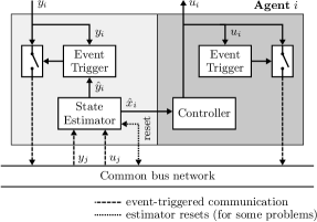
Figure 2: Event-based architecture implemented on each agent of the NCS in Fig. 1. The light-gray area encompasses the blocks used for state estimation. The darker area has additional blocks required when local estimates are used for distributed control.

Remark 3.

To ensure consistent estimates among all agents, the State Estimator in Fig. 2 uses the local measurement $y_{i}$ only when it is also shared over the bus. For the purpose of improving local state estimates, one may wish to incorporate $y_{i}$ in the estimation at every step. For this purpose, a second estimator can be introduced that fuses, at every step, the network data and the local sensor data (see Trimpe and D’Andrea (2011a)).

One possible use of local state estimates is for feedback control. As shown in Fig. 2 (dark-gray area), the estimate is fed to a Controller, which computes inputs $u_{i}$ to the local actuator. With an estimate of the full state at hand, each agent can simply implement (8) for its local actuator to emulate the centralized design; namely

$$u_{i}(k)=F_{i}\hat{x}_{i}(k)$$ (11)

where $F_{i}$ is the part of the gain matrix $F$ in (8) corresponding to its local input $u_{i}$. Since the inputs also need to be available for state estimation, another Event Trigger is employed to manage their communication.

In this section, we shall focus on the event-based estimation problem; that is, the design of the Event Trigger and the State Estimator in the light-gray area in Fig. 2. To develop the main ideas and leaving technical details aside, we consider a simplified scenario first.

3.2 Idealizing assumption

If all estimates $\hat{x}_{i}(0)$ are initialized identically, and the bus communication is perfect (i.e. without any delay and packet drops), all estimates $\hat{x}_{i}$ will be identical. This, we shall assume throughout this section:

Assumption 4.

$\hat{x}_{i}(k)=\hat{x}_{j}(k)$ for all $i,j\in\mathbb{N}_{N}$, $k\in\mathbb{N}$.

Clearly, this assumption is unrealistic in practice because it will be violated by a single packet drop or a slight difference in initialization or computation on any two agents. Thus, we remove it again in Section 4.

Assuming knowledge of the control gain $F$, every agent can reconstruct locally the complete control input vector

$$\hat{u}^{i}(k)=F\hat{x}_{i}(k)$$ (12)

and use it for state prediction (5). Assumption 4 implies that this reconstruction is perfect ($\hat{u}^{i}(k)=u(k)$) and exchange of inputs between agents is thus not necessary. Therefore, we focus solely on the event-based communication of measurements in this section. Communication of inputs and also occasional estimator resets as shown in Fig. 2 shall become relevant later.

3.3 Event trigger

The Event Trigger on agent $i$ (Fig. 2, light-gray) decides at every step $k$, whether or not the local measurement $y_{i}(k)$ is sent to all other agents using the decision rule:

$$\text{transmit $y_{i}(k)$}\;\Leftrightarrow\;\|y_{i}(k)-C_{i}\hat{x}_{i}(k|k-1)\|\geq\delta^{\text{est}}_{i}$$ (13)

where $\delta^{\text{est}}_{i}\geq 0$ is a design parameter, $\hat{x}_{i}(k|k-1)$ is agent $i$’s prediction of the state $x(k)$ based on measurements until time $k-1$ (made precise in the next subsection), and $\hat{y}_{i}(k)=C_{i}\hat{x}_{i}(k|k-1)$ is agent $i$’s prediction of its measurement $y_{i}(k)$. Hence, $y_{i}(k)$ is broadcast if, and only if, the prediction deviates by more than the tolerable threshold $\delta^{\text{est}}_{i}$. Tuning $\delta^{\text{est}}_{i}$ allows the designer to trade off each sensor’s frequency of events (and, hence, the communication rate) for estimation performance. For later reference, we introduce $\delta^{\text{est}}:=(\delta^{\text{est}}_{1},\dots,\delta^{\text{est}}_{N})$.

We denote by $I(k)$ and $\bar{I}(k)$ the indices of those agents transmitting and not transmitting at time $k$; that is,

$$I(k) :=\{i\in\mathbb{N}_{N}\,|\,\|y_{i}(k)-C_{i}\hat{x}_{i}(k|k\!-\!1)\|\geq\delta^{\text{est}}_{i}\}$$ (14)

$$\bar{I}(k) :=\{i\in\mathbb{N}_{N}\,|\,\|y_{i}(k)-C_{i}\hat{x}_{i}(k|k\!-\!1)\|<\delta^{\text{est}}_{i}\}.$$ (15)

3.4 State estimator

Agent $i$’s State Estimator (Fig. 2) recursively computes an estimate $\hat{x}_{i}(k)=\hat{x}_{i}(k|k)$ of the system state $x(k)$ from the all measurements $I(1),\dots,I(k)$ transmitted until time $k$. We propose the following estimator update:

$$\hat{x}_{i}(k|k-1) =A\hat{x}_{i}(k-1|k-1)+B\hat{u}^{i}(k-1)$$ (16)

$$\hat{x}_{i}(k|k) =\hat{x}_{i}(k|k-1)$$

$$\phantom{=}+\!\!\sum_{\ell\in I(k)}\!\!L_{\ell}\big{(}y_{\ell}(k)-C_{\ell}\hat{x}_{i}(k|k-1)\big{)}$$ (17)

where the observer gains $L_{\ell}$ are taken from the centralized design (7), and $\hat{u}^{i}(k-1)$ is agent $i$’s knowledge of the full input vector (here, $\hat{u}^{i}(k-1)=u(k-1)$ from (12) and Assumption 4). Comparing (16), (17) to (5), (7), we see that the estimator structure is the same, but the event-based estimator updates with a subset $I(k)\subset\mathbb{N}_{N}$ of all measurements. If, at time $k$, no measurement is transmitted (i.e. $I(k)=\emptyset$), (17) is to be understood such that the summation vanishes; that is, $\hat{x}_{i}(k|k)=\hat{x}_{i}(k|k-1)$. In order to ease the presentation, this case is not explicitly mentioned hereafter.

3.5 Stability analysis

The estimator equations (16), (17) and the triggering rule (13) together constitute the porposed event-based state estimator (EBSE). For a fixed sequence $I(1),\dots,I(k)$, the estimator (16), (17) is linear. Because the index set $I(k)$ depends on $y(k)$ by (14), however, the EBSE is a nonlinear, switching observer, whose switching modes are governed by the event trigger (13). Stability of the EBSE is discussed next.

Since the main objective is to mimic the centralized reference estimator $\hat{x}_{c}(k)$ (cf. Section 2.3), we first consider the difference $e_{i}(k)=\hat{x}_{c}(k)-\hat{x}_{i}(k)$. Using (5), (7), (16), and (17), straightforward manipulation yields

$$e_{i}(k) =Ae_{i}(k\!-\!1)+\sum\nolimits_{\ell\in\mathbb{N}_{N}}L_{\ell}\big{(}y_{\ell}(k)-C_{\ell}\hat{x}_{\text{c}}(k|k\!-\!1)\big{)}$$

$$\phantom{=}-\!\!\underbrace{\sum\nolimits_{\ell\in I(k)}\!\!L_{\ell}\big{(}y_{\ell}(k)-C_{\ell}\hat{x}_{i}(k|k-1)\big{)}}_{\sum_{\ell\in\mathbb{N}_{N}}\!L_{\ell}(\,\ldots\,)\,\,-\,\,\sum_{\ell\in\bar{I}(k)}\!L_{\ell}(\,\ldots\,)}$$

$$=(I-LC)Ae_{i}(k-1)$$

$$\phantom{=}+\!\!\sum\nolimits_{\ell\in\bar{I}(k)}\!\!L_{\ell}\big{(}y_{\ell}(k)-C_{\ell}\hat{x}_{i}(k|k-1)\big{)}$$ (18)

The error $e_{i}(k)$ is governed by the stable centralized estimator dynamics $(I-LC)A$ with an extra input term, which is essentially bounded by the choice of the event-trigger (13), as can be seen from (15) with $\hat{x}_{i}(k|k-1)=\hat{x}_{\ell}(k|k-1)$. We thus have the following result:

Theorem 5.

Under Assumptions 1 and 4, the difference $e_{i}(k)$ between the centralized estimator and the EBSE (16), (17), and (13) is bounded for all initial conditions $\hat{x}_{i}(0)$ and $x_{\text{{c}}}(0)$. In particular, there exist constants $c>0$ and $\rho\in[0,1)$ such that

$$\|e_{i}\|\leq c\|e_{i}(0)\|+\frac{c}{1-\rho}\|L\|\|\delta^{\text{{est}}}\|.$$ (19)

With Assumption 4, (18) is rewritten as

$$e_{i}(k)=(I-LC)Ae_{i}(k-1)+L_{\bar{I}(k)}\Delta_{\bar{I}(k)}(k)$$ (20)

where $\Delta_{i}(k):=y_{i}(k)-C_{i}\hat{x}_{i}(k|k-1)$, $\Delta_{\bar{I}(k)}(k)$ denotes the vector obtained from stacking $\Delta_{i}(k)$, $i\in\bar{I}(k)$, from top to bottom; and $L_{\bar{I}(k)}$ is obtained from stacking $L_{i}$, $i\in\bar{I}(k)$, from left to right.

By Assumption 1, $e_{i}(k)=(I-LC)Ae_{i}(k-1)$ is exponentially stable, and there exist $c>0$ and $\rho\in[0,1)$ such that $\|((I-LC)A)^{k}\|\leq c\rho^{k}$ for all $k\in\mathbb{N}$ (Callier and Desoer, 1991, p. 212–213). For $1\leq q<\infty$, we find

$$\|\Delta_{\bar{I}(k)}(k)\|_{q}^{q}=\!\!\sum_{i\in\bar{I}(k)}\!\!\|\Delta_{i}(k)\|_{q}^{q}\underset{\eqref{eq:Ibar}}{<}\!\!\sum_{i\in\bar{I}(k)}\!\!(\delta^{\text{est}}_{i})^{q}\leq\|\delta^{\text{est}}\|_{q}^{q},$$ (21)

and, for $q=\infty$,

$$\|\Delta_{\bar{I}(k)}(k)\|_{q}=\!\max_{i\in\bar{I}(k)}\|\Delta_{i}(k)\|_{q}\!\underset{\eqref{eq:Ibar}}{<}\!\max_{i\in\bar{I}(k)}\delta^{\text{est}}_{i}\leq\|\delta^{\text{est}}\|_{q}.$$ (22)

Hence, $\|\Delta_{\bar{I}(k)}(k)\|<\|\delta^{\text{est}}\|$. Since also $\|L_{\bar{I}(k)}\|\leq\|L\|$, the input term $L_{\bar{I}(k)}\Delta_{\bar{I}(k)}(k)$ in (20) is bounded. Using these results and applying (Callier and Desoer, 1991, p. 218, Thm. 75) yields the inequality (19). ∎

The first term in (19), $c\|e_{i}(0)\|$, is due to possibly different initial conditions. As initial conditions will decay exponentially, $\frac{c}{1-\rho}\|L\|\|\delta^{\text{est}}\|$ represents the asymptotic bound. Choosing $\delta^{\text{est}}_{i}$ small enough, $e_{i}(k)$ can hence be made arbitrarily small as $k\to\infty$, and, for $\delta^{\text{est}}_{i}=0$, the performance of the centralized estimator is recovered.

The bound (19) holds irrespective of the representation of the disturbances $v$ and $w$ in (1), (2). In particular, it also holds for the case where the disturbances are unbounded, such as for Gaussian noise. The reason is that Theorem 5 concerns $e_{i}(k)=\hat{x}_{c}(k)-\hat{x}_{i}(k)$, the difference between an agent’s estimate to the (hypothetical) centralized estimator, and the noise will affect both estimates in the same way.

The actual estimation error $\epsilon_{i}$ of agent $i$ is

$$\epsilon_{i}(k) :=x(k)-\hat{x}_{i}(k)=\epsilon_{\text{c}}(k)+e_{i}(k).$$ (23)

Theorem 5 can thus be used to deduce properties of the estimation error $\epsilon_{i}$ from properties of the centralized estimator. For example, in a deterministic setting with bounded disturbances $v$, $w$ and thus bounded $\epsilon_{\text{c}}$, a bound on the estimation error can readily be computed from (23) and Theorem 5. For a stochastic scenario, where $v$, $w$ are zero-mean with known variance, the variance of $\epsilon_{\text{c}}$ can be determined using standard methods, and (23) and Theorem 5 can then be used to compute a bound on the variance of $\epsilon_{i}$.

3.6 Remote estimation scenario

While Assumption 4 is unrealistic for a multi-agent scenario, it is trivially satisfied when there is only one agent. An example scenario is shown in Fig. 3. Therein, a sensor agent observes a dynamic process and sporadically transmits measurements to a remote agent, which computes state estimates for monitoring purposes, for example. The remote estimator thus implements the state estimator (16), (17). The sensor node also implements (16), (17), as well as the event trigger (13) for making the transmit decisions.

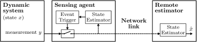
Figure 3: Remote estimation scenario with a single sensor.

The stability analysis of this section directly applies to the stability of the estimator on the sensor node. If communication from sensor to remote estimator is perfect, the remote estimate is the same as the estimate at the sensor. However, even if the communication is disturbed, this does not impair stability. While the disturbance will clearly affect the remote estimate, this one, in turn, has no effect on the estimate at the sensor and thus future transmit decisions. This is fundamentally different for the distributed arrangement as in Fig. 1, where each of the agents computes estimates and makes transmit decisions based on these. Agents thus influence each other, and stability can actually be lost if two agents’ estimates differ, as is discussed in the next section.

4 Distributed Event-based State Estimation

In this section, we take up the main ideas from the previous section, but address two aspects relevant for a distributed implementation in practice. First, we remove the unrealistic Assumption 4 and analyze stability when agents’ estimates can differ ($\hat{x}_{i}(k)\not=\hat{x}_{j}(k)$). Second, we treat the communication of the inputs $u$.

4.1 Event-based communication of inputs

Knowledge of the control input $u$ is required in the estimator update (16). In the previous section, this was trivially achieved since, by Assumption 4, every agent can compute every other agent’s input exactly from its local estimate. If this is not the case, one has different options. First, all agents could communicate their input (11) periodically over the bus. While this increases network load, it can be a viable option if the number of inputs is comparably small. Second, each agent could estimate the full input vector according to (12); without Assumption 4, this only yields an approximation of the true input ($\hat{u}^{i}(k)\approx u(k)$). It can be shown that the separation principle does not hold for this information pattern even for periodic communication; that is, Assumptions 1 and 2 are not sufficient for stability. Notwithstanding, it is possible to specifically design observer gains to achieve closed-loop stability, (Muehlebach and Trimpe, 2015). Since herein, we seek to mimic the centralized observer (5), (6) without changing its gain $L$, we opt for a third alternative, where inputs are shared over the common bus, but according to an event-based protocol.

The Controller in Fig. 2 implements (11) to compute the local input $u_{i}$. The corresponding Event Trigger uses the following rule to decide when to broadcast $u_{i}$:

$$\text{transmit $u_{i}(k)$}\;\;\Leftrightarrow\;\;\|u_{i}(k)-u_{i,\text{last}}(k)\|\geq\delta^{\text{{ctrl}}}_{i}$$ (24)

where $\delta^{\text{{ctrl}}}_{i}\geq 0$ is a tuning parameter, and $u_{i,\text{last}}(k)$ is the last input that was sent. That is, we employ a simple send-on-delta scheme for input communication. Analogous to Section 3.3, we define

$$I^{\text{ctrl}}(k) :=\big{\{}i\in\mathbb{N}_{N}\,|\,\|u_{i}(k)-u_{i,\text{last}}(k)\|\geq\delta^{\text{{ctrl}}}_{i}\big{\}}$$ (25)

and $\delta^{\text{{ctrl}}}:=(\delta^{\text{{ctrl}}}_{1},\dots,\delta^{\text{{ctrl}}}_{N})$.

Each agent keeps track of the last known inputs of all other agents. Agent $i$’s estimate of agent $j$’s input is

$$\hat{u}^{i}_{j}(k)=\begin{cases}u_{j}(k)&\text{if \eqref{eq:eventTriggerCtrl} triggered}\\ \hat{u}^{i}_{j}(k-1)&\text{otherwise}.\end{cases}$$ (26)

Accordingly, all agents use $\hat{u}^{i}(k-1)=(\hat{u}^{i}_{1}(k-1),\hat{u}^{i}_{2}(k-1),\dots,\hat{u}_{N}(k-1))$ as estimate of the full input vector for the estimator update (16). Since all agents use the same input vector estimate, we write $\hat{u}(k)=\hat{u}^{i}(k)$ for simplicity. For the input estimation error $\tilde{u}(k):=u(k)-\hat{u}(k)$, the following is immediate:

Lemma 6.

$\|\tilde{u}\|_{\infty}\leq\|\delta^{\text{{ctrl}}}\|$.

Remark 7.

Each agent uses the last communicated value $\hat{u}_{i}(k-1)$ of its own input $u_{i}(k-1)$ in the estimator update, even though the true input $u_{i}(k-1)$ could be used instead. This is analogous to not always using the latest local measurement in the estimator (cf. Remark 3) in order to keep consistent estimates. However, the true local input can also be used in the estimator update with only slight modification of the following derivations.

4.2 Inter-agent differences

To account for differences in the agents’ estimates (i.e. removing Assumption 4), we introduce a disturbance signal $d_{i}$ in each estimate and replace (17) with

$$\hat{x}_{i}(k|k) =\hat{x}_{i}(k|k\!-\!1)\!+\!\sum\nolimits_{\ell\in I(k)}\!\!\!\!\!L_{\ell}\big{(}y_{\ell}(k)-C_{\ell}\hat{x}_{i}(k|k\!-\!1)\big{)}$$

$$\phantom{=}+d_{i}(k).$$ (27)

The disturbance $d_{i}$ may stem from, for example, unequal initialization, different computation accuracy, or imperfect communication of measurements or inputs.

Remark 8.

We emphasize that the disturbance $d_{i}$ is introduced in (27) solely for the purpose of analysis. When implementing the estimator, (17) is used in the sense that all measurements received by agent $i$ at time $k$ are included in the summation. Packet drops can be represented through $d_{i}$ as follows: if $y_{\ell}(k)$, $\ell\in I(k)$ is a measurement not received at agent $i$, then $d_{i}(k)=-L_{\ell}(y_{\ell}(k)-C_{\ell}\hat{x}_{i}(k|k-1))$ accounts for the lost packet.

For the following analysis, we assume bounded disturbances:

Assumption 9.

For all $i\in\mathbb{N}_{N}$, $\|d_{i}\|_{\infty}\leq d_{i}^{\text{{max}}}$.

This assumption is realistic, when $d_{i}$ represents imperfect initialization or imprecise computations, for example. Even though the assumption may not hold for the case of modeling packet drops in general, the developed method was found to be effective also for this scenario in the simulation examples of Section 6.

With (26) and (27), the error (18) becomes

$$e_{i}(k)=(I-LC)Ae_{i}(k-1)+(I-LC)B\tilde{u}(k-1)$$

$$\phantom{=}+\!\sum\nolimits_{\ell\in\bar{I}(k)}\!\!L_{\ell}\big{(}y_{\ell}(k)-C_{\ell}\hat{x}_{i}(k|k-1)\big{)}-d_{i}(k).$$ (28)

The key difficulty that arises for the stability analysis is that the event-triggers (13) bound the difference $\|y_{i}(k)-C_{i}\hat{x}_{i}(k|k-1)\|$ for agent $i$, but not the difference $\|y_{\ell}(k)-C_{\ell}\hat{x}_{i}(k|k-1)\|$ for $\ell\not=i$ as appearing in (28). Hence, it can no longer be directly concluded that the sum in (28) is bounded. To obtain further insight, we rewrite (28) as

$$e_{i}(k) =(I-LC)Ae_{i}(k-1)+(I-LC)B\tilde{u}(k-1)$$

$$\phantom{=}+\!\!\sum\nolimits_{\ell\in\bar{I}(k)}\!\!L_{\ell}\big{(}y_{\ell}(k)-C_{\ell}\hat{x}_{\ell}(k|k-1)\big{)}-d_{i}(k)$$

$$\phantom{=}-\!\!\sum\nolimits_{j\in\bar{I}(k)}\!\!L_{j}C_{j}Ae_{ij}(k-1)$$ (29)

where $e_{ij}(k)=\hat{x}_{i}(k)-\hat{x}_{j}(k)$ is the inter-agent error; we used $\hat{x}_{i}(k|k-1)-\hat{x}_{\ell}(k|k-1)=Ae_{i\ell}(k-1)$; and we substituted index $j$ for $\ell$ in the last term. In contrast to the simplified analysis in Section 3, agent $i$’s estimation error $e_{i}$ now depends on the other estimates through $e_{ij}$. Except for the term $\sum_{j\in\bar{I}(k)}L_{j}C_{j}Ae_{ij}(k-1)$, all other input terms are bounded by (15), Assumption 9, and Lemma 6. Thus, for establishing stability, the inter-agent error $e_{ij}(k-1)$ must be bounded.

The inter-agent error dynamics are given by

$$e_{ij}(k) =\hat{x}_{i}(k)-\hat{x}_{j}(k)=Ae_{ij}(k-1)$$

$$\phantom{=}+\sum\nolimits_{\ell\in I(k)}L_{\ell}\big{(}y_{\ell}(k)-C_{\ell}\hat{x}_{i}(k|k-1)\big{)}+d_{i}(k)$$

$$\phantom{=}-\sum\nolimits_{\ell\in I(k)}L_{\ell}\big{(}y_{\ell}(k)-C_{\ell}\hat{x}_{j}(k|k-1)\big{)}-d_{j}(k)$$

$$=\tilde{A}_{I(k)}\,e_{ij}(k-1)+d_{i}(k)-d_{j}(k)$$ (30)

where $\tilde{A}_{I(k)}:=(I-\sum_{\ell\in I(k)}L_{\ell}C_{\ell})A$ was introduced for brevity. The inter-agent error $e_{ij}(k)$ is governed by the unforced time-varying dynamics $e_{ij}(k)=\tilde{A}(k)e_{ij}(k-1)$. In general, one cannot infer stability of the event-based scheme from stability of the centralized design (Assumption 1) as was done in Section 3 by disregarding inter-agent errors. In fact, an example is presented in Section 6.1 where the inter-agent differences destabilize the event-based system despite stability of the centralized estimator. If, however, the time-varying dynamics $e_{ij}(k)=\tilde{A}_{I(k)}e_{ij}(k-1)$ can be shown to be stable for a specific design $L$, boundedness of $e_{ij}(k)$ can be concluded. Such an example is presented in Section 6.2.

Next, we present a straightforward extension of the event-based communication scheme, which guarantees stability for an arbitrary centralized observer gain $L$.

4.3 Synchronous averaging mechanism

Since the inter-agent error $e_{ij}(k)$ is the difference between the state estimates by agent $i$ and $j$, we have full control over it: we can make it zero at any time by resetting the two agents’ state estimates to the same value, for example, their average. Therefore, a straightforward way to guarantee bounded inter-agent errors is to periodically reset all agents’ estimates to their joint average. Clearly, this strategy increases the communication load on the network. If, however, the disturbances $d_{i}$ are small or only occur rarely, the required resetting period can be large relative to the underlying sampling time $T_{s}$.

We assume that the resetting happens after all agents have made their estimator updates (27). Let $\hat{x}_{i}(k-)=\hat{x}_{i}(k)$ and $\hat{x}_{i}(k+)$ denote agent $i$’s estimate before and after resetting, and let $K\in\mathbb{N}$ be the fixed resetting period. Each agent $i$ implements the following synchronous averaging mechanism:

If $$k K \hat{x}_{i}(k-)$$ a multiple of : transmit ; (31)

receive $$\hat{x}_{j}(k-),j\in\mathbb{N}_{N}\!\setminus\!\{i\}$$;

set $$\hat{x}_{i}(k+)=\operatorname*{avg}\nolimits_{j=1,\dots,N}(\hat{x}_{j}(k-))$$

We assume that the network capacity is such that the mutual exchange of the estimates can happen in one time step (as is the case for the system in Trimpe (2012)), and that no data is lost in the transfer (e.g. through appropriate low-level protocols using acknowledgments). In other scenarios, one could take several time steps to exchange all estimates, at the expense of a delayed reset. Alternatives to resetting the average are also conceivable, such as resetting to the estimate of one particular agent.

The synchronous averaging period $K$ can be chosen from simulations assuming a model for the inter-agent disturbances $d_{i}$ (e.g. packet drops). In a typical design procedure, an event-based design is carried out first making the idealizing assumption of zero inter-agent errors (according to Section 3). The triggering thresholds $\delta^{\text{est}}_{i}$ are adjusted such that a desirable trade-off between communication and estimation performance is obtained. In a second stage, (31) is introduced, and $K$ is chosen so as to keep inter-agent errors small.

Remark 10.

The synchronous averaging (31) requires exchange of estimates between agents, which is in addition to the event-based communications (13) and (24). Even though a stable estimation scheme with the synchronous exchange of estimates alone would be conceivable, this would typically require relatively high update rates. The design herein primarily relies on event-based communication. The synchronous averaging mechanism is introduced just to keep inter-agent errors small and guarantee stability under practical circumstances. In a scenario, where inter-agent differences occur infrequently, the synchronous resetting frequency can be small and most communication is due to the event-triggering.

4.4 Stability result

With the augmentation of the previous subsection, we can now establish a bounded difference between the EBSE and the centralized reference estimator.

Theorem 11.

Under Assumptions 1 and 9, the difference $e_{i}(k)$ between the centralized estimator and the EBSE given by (16), (26), (27), (13), (24), and (31) is bounded for all initial conditions $\hat{x}_{i}(0)$ and $x_{\text{{c}}}(0)$.

Since the agent error dynamics (29) will be affected by the resetting (31), we first rewrite the error dynamics in terms of the average estimate $\bar{x}(k):=\operatorname*{avg}(\hat{x}_{i}(k))$. Defining the errors $\bar{e}(k):=\hat{x}_{\text{c}}(k)-\bar{x}(k)$ and $\bar{e}_{i}(k):=\bar{x}(k)-\hat{x}_{i}(k)$, we have $e_{i}(k)=\bar{e}(k)+\bar{e}_{i}(k)$ and will establish the claim by showing boundedness of $\bar{e}_{i}(k)$ and $\bar{e}(k)$ separately.

For the average estimate $\bar{x}(k)$, we obtain from (16), (27),

$$\bar{x}(k|k-1)=A\bar{x}(k-1)+B\hat{u}(k-1)$$

$$\bar{x}(k)=\bar{x}(k|k\!-\!1)+\!\!\!\sum_{\ell\in I(k)}\!\!L_{\ell}\big{(}y_{\ell}(k)-C_{\ell}\bar{x}(k|k\!-\!1)\big{)}+\bar{d}(k)$$

where $\bar{x}(k|k-1):=\operatorname*{avg}(\hat{x}_{i}(k|k-1))$ and $\bar{d}(k):=\operatorname*{avg}(d_{i}(k))$. The dynamics of the error $\bar{e}_{i}(k)$ are described by

$$\bar{e}_{i}(k) =\tilde{A}_{I(k)}\bar{e}_{i}(k-1)+\bar{d}(k)-d_{i}(k)$$ (32)

$$\bar{e}_{i}(k+) =0,\qquad\text{for $k=\kappa K$ with some $\kappa\in\mathbb{N}$}$$ (33)

where (32) is obtained by direct calculation analogous to (30), and (33) follows from (31). That is, $\bar{e}_{i}$ is periodically reset to $0$ and evolves according to (32) in-between resetting instants. Since $\bar{d}(k)$, $d_{i}(k)$, and $\tilde{A}_{I(k)}$ are all bounded, boundedness of $\bar{e}_{i}$ for all $i\in\mathbb{N}_{N}$ follows.

Since $\bar{e}(k)=\operatorname*{avg}_{i}(e_{i}(k))$, we obtain from (29)

$$\bar{e}(k) =(I-LC)A\bar{e}(k-1)+(I-LC)B\tilde{u}(k-1)$$

$$\phantom{=}+\!\!\sum\nolimits_{\ell\in\bar{I}(k)}\!\!L_{\ell}\big{(}y_{\ell}(k)-C_{\ell}\hat{x}_{\ell}(k|k-1)\big{)}-\bar{d}(k)$$

$$\phantom{=}-\!\!\sum\nolimits_{j\in\bar{I}(k)}\!\!L_{j}C_{j}A\bar{e}_{j}(k-1)$$ (34)

where we used $\operatorname*{avg}_{i}(e_{ij}(k))=\operatorname*{avg}_{i}(\hat{x}_{i}(k)-\hat{x}_{j}(k))=\bar{x}(k)-\hat{x}_{j}(k)=\bar{e}_{j}(k)$. Note that (34) fully describes the evolution of $\bar{e}(k)$. In particular, the resetting (31) does not affect $\bar{e}(k)$ because, at a resetting instant $k=\kappa K$, it holds that $\bar{e}(k+)=\hat{x}_{\text{c}}(k)-\frac{1}{N}\sum\nolimits_{j=1}^{N}\hat{x}_{j}(k+)=\hat{x}_{\text{c}}(k)-\frac{1}{N}\sum\nolimits_{j=1}^{N}\big{(}\frac{1}{N}\sum\nolimits_{\ell=1}^{N}\hat{x}_{\ell}(k-)\big{)}=\hat{x}_{\text{c}}(k)-\frac{1}{N}\sum\nolimits_{\ell=1}^{N}\hat{x}_{\ell}(k-)=\bar{e}(k-)$. All input terms in (34) are bounded: $\tilde{u}$ by Lemma 6, $\bar{d}$ by Assumption 9, $\sum_{\ell\in\bar{I}(k)}L_{\ell}(y_{\ell}(k)-C_{\ell}\hat{x}_{\ell}(k|k-1))$ by the event-triggering mechanism (see (15)), and $\bar{e}_{j}$ for all $j$ by the previous argument. Since $z(k)=(I-LC)Az(k-1)$ is exponentially stable, it follows that $\bar{e}(k)$ is bounded for all $k$ (Callier and Desoer, 1991, Thm. 75, p. 218), which completes the proof.  ∎

By means of Theorem 11 and (23), properties about the agent’s estimation error $\epsilon_{i}(k)=x(k)-\hat{x}_{i}(k)$ can readily be derived given properties of the disturbances $v$, $w$, and the centralized estimator. The discussion in Section 3.5 applies analogously. An upper bound on $\epsilon_{i}(k)$ in terms of the problem parameters corresponding to (19) can be derived for Theorem 11; it is omitted here for simplicity. If the inter-agent errors are small, the simpler bound (19) may be used for all practical purposes.

5 Distributed Event-based Control

In this section, we discuss stability of the full distributed, event-based control system shown in Fig. 2, where the estimate $\hat{x}_{i}$ is used for control. Algorithm 1 summarizes the implementation of the complete event-based control system on each agent.

Algorithm 1 Implementation on agent $i$, executed every time step $k$.

Actuation: apply $u_{i}(k-1)$
Sensing: acquire $y_{i}(k)$
Estimation:
	Prediction (16): compute $\hat{x}_{i}(k|k-1)$
	Measurement trigger (13): send/receive $y_{\ell}(k),\ell\in I(k)$
	Measurement update (17): compute $\hat{x}_{i}(k|k)=\hat{x}_{i}(k)$
	if ($k$ is a multiple of $K$)
		perform synchronous reset (31)
	end if
Control:
	Control law (11): compute $u_{i}(k)$ from $\hat{x}_{i}(k)$
	Control trigger (24): send/receive $u_{\ell}(k),\ell\in I^{\text{ctrl}}(k)$

Closed-loop stability can be deduced from stability of the event-based estimation (Theorem 11) and of the centralized control system (Assumption 2).

Theorem 12.

Let $v$ and $w$ be bounded, and let assumptions 1, 2, 9 be satisfied. Then, the state $(x(k)$, $\epsilon_{1}(k)$, $\epsilon_{2}(k),\dots,\epsilon_{N}(k))$ of the distributed event-based control system given by (1), (2), (11), (16), (26), (27), (13), (24), (31) is bounded for all initial conditions $\hat{x}_{i}(0)$ and $x(0)$.

From Assumption 1 with bounded $v$ and $w$, it follows that the estimation error $\epsilon_{\text{c}}(k)$ of the centralized observer is bounded (cf. (10)). Thus, (23) and Theorem 11 imply that all $\epsilon_{i}$, $i\in\mathbb{N}_{N}$, are bounded. Using (11) and (23), we rewrite (3) as $x(k)=(A+BF)x(k\!-\!1)-\!\sum_{i\in\mathbb{N}_{N}}B_{i}F_{i}\epsilon_{i}(k\!-\!1)+v(k\!-\!1)$. Hence, it follows from stability of $A+BF$ (Assumption 2) and bounded $v$ that $x$ is also bounded.  ∎

6 Illustrative Examples

The proposed methods for distributed event-based estimation and control are illustrated by means of two simulations examples: a simulation model of the Balancing Cube test bed (Trimpe and D’Andrea, 2012a), which was also used for the experiments in (Trimpe, 2012), as well as a thermo-fluid process benchmark problem (Grüne et al., 2014). Matlab files to run both simulation examples are provided as supplementary material.

6.1 Balancing Cube

The Balancing Cube is a dynamic sculpture that can balance on any one of its edges or corners by means of six rotating arms attached to its structure. The arms constitute the agents of the NCS as in Fig. 1. The system was developed as a test bed for distributed estimation and control and used, among others, to demonstrate the event-based algorithms herein, (Trimpe, 2012).

6.1.1 System description

A state-space model (1) of the cube’s linearized dynamics when balancing on an edge is given in (Trimpe and D’Andrea, 2012b, Eq. (3)). Analogous to the implementation in (Trimpe, 2012), we exploit the model structure to obtain a reduced-state model for estimator design:

$$x(k)=Ax(k\!-\!1)+B_{1}u(k\!-\!1)+B_{2}u(k\!-\!2)+v(k\!-\!1)$$

$$\quad A=\begin{bmatrix}I&0\\[-3.44444pt] A_{31}&A_{33}\end{bmatrix}\!,\,B_{1}=\begin{bmatrix}T_{\text{s}}I\\[-3.44444pt] B_{3}\end{bmatrix}\!,\,B_{2}=\begin{bmatrix}0\\[-3.44444pt] A_{32}\end{bmatrix}$$ (35)

with sampling time $T_{\text{s}}=0.01\,\text{s}$, $I$ and $0$ identity and zero-matrices, and the numerical values of the other matrices given in (Trimpe and D’Andrea, 2012b). The model includes the effect of local velocity feedback on each agent, and the inputs $u$ are the reference velocities to these local controllers. The special structure of this model follows from a time-scale separation algorithm assuming sufficiently fast velocity feedback loops (see (Trimpe and D’Andrea, 2012a) for details). The states and inputs of the model (35) are summarized in Table 1.

Table 1: States and inputs of the Balancing Cube model.

States		Unit
$x_{1},\dots,x_{6}$	angle arm 1 to 6	rad
$x_{7}$	angle cube body	rad
$x_{8}$	angular velocity cube body	$\text{rad}/\text{s}$
Inputs		Unit
$u_{1},\dots,u_{6}$	reference angular velocity	$\text{rad}/\text{s}$

The output equation (2) is

$$y(k) =\begin{bmatrix}y_{1}(k)\\[-3.44444pt] \vdots\\[-3.44444pt] y_{9}(k)\end{bmatrix}=\left[\begin{smallmatrix}1&0&0&0&0&0&0&0\\ 0&0&0&0&0&0&0&1\\ 0&1&0&0&0&0&0&0\\ 0&0&0&0&0&0&0&1\\ 0&0&1&0&0&0&0&0\\ 0&0&0&0&0&0&0&1\\ 0&0&0&1&0&0&0&0\\ 0&0&0&0&1&0&0&0\\ 0&0&0&0&0&1&0&0\\ \end{smallmatrix}\right]x(k)+w(k)$$ (36)

which is in accordance with the sensors on the physical system (angle encoders for the six arms $y_{1}$, $y_{3}$, $y_{5}$, $y_{7}$, $y_{8}$, $y_{9}$, and rate gyroscopes $y_{2}$, $y_{4}$, $y_{6}$). Inputs and outputs as associated to the six agents are summarized in Table 2. As is easily checked (see supplementary files), the state $x$ is not detectable from the sensors of any individual agent. Inter-agent communication is therefore necessary for stable state estimation.

Table 2: Agents of the Balancing Cube model.

Agent #	1	2	3	4	5	6
Actuator	$u_{1}$	$u_{2}$	$u_{3}$	$u_{4}$	$u_{5}$	$u_{6}$
Sensors	$y_{1}$, $y_{2}$	$y_{3}$, $y_{4}$	$y_{5}$, $y_{6}$	$y_{7}$	$y_{8}$	$y_{9}$

The noise variables $v(k)$ and $w(k)$ are modeled as independent uniform random variables. The sensor noise variance is chosen comparable to the sensors on the actual system (noise on angle measurements is negligible, noise on angular rate sensors is significant). To account for non-ideal actuation, we simulate input noise, uniformly distributed in $[-0.05,0.05]\,\text{rad/s}$. For any measurement $y_{i}(k)$ transmitted over the network, a packet drop probability of 2% is modeled. Dropped measurements can be expressed by the disturbance signal $d_{i}$ as explained in Remark 8. For simplicity, we assume that inputs and synchronous resetting are not affected by data loss.

6.1.2 Event-based estimation and control system design

Each agent implements Algorithm 1, but in slight deviation thereof, agents 1 to 3 make individual triggering decisions for each of their two sensors. For example, Agent 2 implements the trigger (13) separately for $y_{3}$ and $y_{4}$. Advantages are greater potential for reducing the amount of transmitted data and different units are handled naturally. In other scenarios such as networks allowing for large packet sizes, sending all measurements at once may be preferred. The proposed framework can accommodate for these different communication architectures.

To implement the event-based estimation and control scheme, observer and controller gains, and the communication thresholds need to be chosen. The centralized observer (5), (6) is designed as a steady-state Kalman filter with eigenvalues of the error dynamics $(I-LC)A$ at $0.97$, $0.96$, and $0.73$ (sixfold). The centralized controller (8) is obtained from an LQR design guaranteeing stability of $A+BF$ (see supplementary material for details). We chose the following triggering thresholds: $\delta^{\text{est}}_{\text{gyro}}=0.004\,\text{rad}/\text{s}$ for the rate gyro sensors ($y_{2}$, $y_{4}$, $y_{6}$), $\delta^{\text{est}}_{\text{enc}}=0.001\,\text{rad}$ for the encoders (all other $y_{i}$), and $\delta^{\text{{ctrl}}}=0.01\,\text{rad}/\text{s}$ for all inputs. In this example, we shall see that synchronous averaging (31) is required for stability. We chose $K=200$ as the reset period (every $2\,\text{s}$).

6.1.3 Simulation results

Figure 4 shows selected state and error signals from simulating the event-based control system as described in Section 6.1.2. The error signals are given for agent 2; both the actual estimation error $\epsilon_{2}$ and the difference $e_{2}$ to the centralized reference estimator are shown. The difference $e_{2}$ to the centralized estimate is guaranteed to be bounded by Theorem 11. The results show that the effective bounds on the arm angles (black and blue graphs) are in the order of the triggering threshold $\delta^{\text{est}}_{\text{enc}}=0.001\,\text{rad}$. In general, however, the bounds depend not only on the trigger thresholds, but also the error dynamics as per (29).

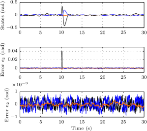
Figure 4: Simulation of the Balancing Cube model. From top to bottom: states $x$, estimation errors $\epsilon_{2}$ of agent 2, and its difference $e_{2}$ to a centralized estimate. In each graph, three signals are shown: the angles of arm 2 (black), arm 5 (blue), and the cube structure (orange).

At $10\,\text{s}$, an impulsive disturbance was applied at the input of agent 2. From the corresponding communication rates given in Fig. 5, a temporary increase in communication can be observed in response to the disturbance. Also visible in Fig. 5 is that encoder and input communication rates are generally lower than those for the rate gyro sensors. This can be expected as the rate gyros are responsible for observing the unstable mode of the system. In general, the event-based design is effective in adapting communication: when there is need for feedback (e.g. disturbances or unstable modes), rates go up.

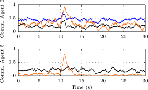
Figure 5: Event-based communication rates for two agents in the cube example. Black: encoder measurements; blue: rate gyro measurements (Agent 5 has no such sensor); orange: control inputs. All rates as moving average over 100 steps.

Figure 6 shows one component of the inter-agent error $e_{15}$; that is, the difference between the estimates of agent 1 and 5. The black graph corresponds to a short sequence of the same simulation run as in Fig. 4 and 5. Synchronous averaging (31) with $K=200$ causes all inter-agent errors to reset to zero every $2\,\text{s}$. In contrast, the orange graph corresponds to a simulation run with (31) disabled ($K\to\infty$). Obviously, the inter-agent error drifts meaning the estimates of the two agents slowly deviate, which eventually destabilizes the whole closed-loop system. With synchronous resetting, however, the inter-agent errors $e_{ij}$ are an order of magnitude smaller than the estimation errors $e_{i}$ or $\epsilon_{i}$ (cf. Fig. 4 and 6). Thus, one can use the simplification of Section 3 for the purpose of analyzing the performance of the system. Yet, for stability, considering non-zero inter-agent errors is critical as this example highlights. In contrast to this example, the thermo-fluid example in Section 6.2 is one where synchronous resetting is found to be unnecessary.

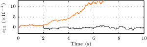
Figure 6: Inter-agent error $e_{15}$ between agents 1 and 5 (one component). Black: with synchronous averaging; orange: without.

6.1.4 Estimation versus communication trade-off

The event-based estimation scheme herein allows the designer to trade off estimation performance for communication by choosing the triggering thresholds. We illustrate this trade-off by performing simulations for different choices of the thresholds. For this, the previously chosen thresholds (Section 6.1.2) are multiplied with a factor varying from 0 to 3 on a logarithmic scale. For each parameter setting, we perform 100 independent simulation runs and compute normalized measures for estimation and communication. The normalized estimation error $\mathcal{E}$ is defined as the squared error $\epsilon_{i}^{\text{T}}\!(k)\epsilon_{i}(k)$, averaged over simulation horizon, all agents, and simulation runs. The normalized communication $\mathcal{C}$ is obtained by averaging the number of transmitted scalars (measurements, inputs, resets) such that $\mathcal{C}=1$ corresponds to full periodic communication of all measurements and inputs, and $\mathcal{C}=0$ to no communication. The obtained $\mathcal{E}$-vs-$\mathcal{C}$ graph is shown in Fig. 7 for the event-based communication design (orange), in comparison to periodic communication (black). The periodic communication graph corresponds to communicating inputs and measurements at multiples of the discrete sampling time $T_{\text{s}}$ (i.e., $1T_{\text{s}}$, $2T_{\text{s}}$, $3T_{\text{s}}$, etc). Controller and observer gains are recomputed for the re-sampled discrete-time model.

While for full communication $\mathcal{C}=1$ both designs yield the same error as expected, event-based communication is superior for lower communications; roughly 80% communication can be saved before experiencing any significant increase in the estimation error. Yet, for very low communication, slow periodic sampling is superior in this example. In general, the trade-off is multi-dimensional due to multiple triggering thresholds, while Fig. 7 only represents one dimension. Nonetheless, this example shows the potential of event-based sampling to make better average use of available communication resources than standard periodic sampling.

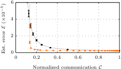
Figure 7: Estimation error versus communication trade-off for event-based (orange) and periodic communication (black). The error bars represent plus/minus one standard deviation of the obtained values for $\mathcal{E}$ from 100 simulation runs. The variability in $\mathcal{C}$ is comparably small and thus not shown.

6.2 Thermo-fluid process

As a second example, we consider distributed event-based control of a thermo-fluid process. In contrast to the previous example, no synchronous resetting is necessary here. The process has been proposed as a benchmark problem for event-based control by Grüne et al. (2014), and used to demonstrate different event-based methods in (Stöcker et al., 2013; Sigurani et al., 2015), for example.

The key components of the plant are two tanks containing fluids, whose level and temperature are to be regulated by controlling the tanks’ inflows, as well as heating and cooling units. Both tanks are subject to step-like disturbances, and their dynamics are coupled through cross-flows between the tanks. Each tank is associated with a control agent responsible for computing commands to the respective actuators. Each agent can sense the temperature and level of its tank. For details on the physical process, including diagrams and photos, the reader is referred to (Grüne et al., 2014; Sigurani et al., 2015).

6.2.1 System description

The discrete-time linear model (1), (2) representing the thermo-fluid process dynamics about an equilibrium configuration is obtained by zero-order hold discretization with a sampling time $T_{\text{s}}=0.2\,\text{s}$ of the continuous-time model given in (Grüne et al., 2014, Sec. 5.8). In contrast to the Balancing Cube example, the process dynamics are stable. The states and inputs of the system are summarized in Table 3. Same as Sigurani et al. (2015), we consider step-wise process disturbances $v(k)$ from exogenous inflow and heating. Noisy measurements $y(k)\in\mathbb{R}^{4}$ of all states are available (i.e. $C=I$ in (2)), and sensor noise $w(k)$ is modeled as uniformly distributed random variable. The numerical parameters of the model are available in the supplementary files.

Table 3: States and inputs of the thermo-fluid process.

States		Unit
$x_{1}(k)$	level tank 1	m
$x_{2}(k)$	temperature tank 1	K
$x_{3}(k)$	level tank 2	m
$x_{4}(k)$	temperature tank 2	K
Inputs		Unit
$u_{11}(k)$	inflow tank 1	1 (normalized)
$u_{12}(k)$	cooling tank 1	1 (normalized)
$u_{21}(k)$	inflow tank 2	1 (normalized)
$u_{22}(k)$	heating tank 2	1 (normalized)

Similar to the distributed architecture in Sigurani et al. (2015), we consider two agents (one for each tank) exchanging data with each other over a network link. Agent 1 measures $y_{1}$ (level) and $y_{2}$ (temperature) of its tank and is responsible for controlling $u_{1}=(u_{11},u_{12})$ (inflow and cooling); and Agent 2 accordingly. The agents’ associated sensors and actuators are summarized in Table 4.

Table 4: Agents in the thermo-fluid example.

Agent #	1	2
Actuator	$u_{1}=(u_{11},u_{12})$	$u_{2}=(u_{21},u_{22})$
Sensors	$y_{1}$, $y_{2}$	$y_{3}$, $y_{4}$

In order to study the effect of imperfect communication, we simulate random packet drops. Any measurement $y_{i}(k)$ that is transmitted between the two agents is lost with a probability of 5%, independent of previous drops. Packet drops are represented by the disturbance $d_{i}(k)$ in (27) as discussed in Remark 8. For simplicity, we assume that inputs when communicated are never lost.

6.2.2 Event-based estimation and control system design

Each agent implements Algorithm 1. As in the example in Section 6.1, triggering decisions are made individually for the two sensors of each agent (cf. Table 4). However, to illustrate the flexibility of the proposed scheme, the triggering decision (24) is applied jointly for both inputs; for example, agent 2 makes the transmit decision jointly for $u_{2}=(u_{21},u_{22})$.

For the design of the centralized observer (5), (6), we chose $L=$ $\operatorname*{diag}(0.1,0.05,0.1,0.05)$ as observer gain, leading to stable centralized estimator dynamics $(I-LC)A$ with eigenvalues approximately at 0.95 and 0.9 (each one twice). As it turns out, for this choice for $L$, also the switching inter-agent error dynamics (30) are stable, which can be seen as follows. By direct calculation, one can verify that

$$\tilde{A}_{J}^{\text{T}}P\tilde{A}_{J}-P<0\quad\text{with}\,\,\tilde{A}_{J}:=(I-\sum\nolimits_{\ell\in J}L_{\ell}C_{\ell})A$$ (37)

is satisfied for $P=\operatorname*{diag}(500,1,500,1)$ and for all permutations $J\subseteq\{1,2,3,4\}$. Thus, it follows that $V(z)=z^{\text{T}}Pz$ is a common Lyapunov function (see Mignone et al. (2000)) for the switching system $z(k)=\tilde{A}_{J(k)}z(k-1)$ for arbitrary $J(k)\subseteq\{1,2,3,4\}$, and, in particular, for $J(k)=I(k)$. It thus follows that the unforced dynamics in (30) are exponentially stable, which implies boundedness of $e_{ij}$. Hence, synchronous averaging (31) is not necessary in this example (in contrast to the one in Section 6.1).

The state-feedback gain $F$ is obtained from a centralized LQR design (Åström and Wittenmark, 1997). In contrast to the decentralized design in (Sigurani et al., 2015), the controller involves full couplings between all states. Using a centralized control design with arbitrary couplings is made possible by maintaining an estimate of the full state on each agents in the propose architecture.

Finally, the triggering thresholds in (13) and (24) are set to $\delta^{\text{est}}_{1}=\delta^{\text{est}}_{3}=0.01\,\text{m}$, $\delta^{\text{est}}_{2}=\delta^{\text{est}}_{4}=0.2\,\text{K}$, and $\delta^{\text{{ctrl}}}_{1}=\delta^{\text{{ctrl}}}_{3}=0.02$.

6.2.3 Simulation results

The state trajectories of a $2000\,\text{s}$ simulation run under event-based communication are shown in Fig. 8. For comparison with the event-based estimates (orange), also the centralized estimate (blue) is shown. Step-wise disturbances $v$, active from $200\,\text{s}$ to $600\,\text{s}$ and from $1000\,\text{s}$ to $1200\,\text{s}$ (gray shaded areas) with comparable magnitudes as in (Sigurani et al., 2015), cause the states to deviate from the equilibrium $x=0$. Especially at times when disturbances are active, the event-based estimate is inferior to the centralized one as is expected due to the reduced number of measurements. However, Theorem 11 guarantees that this difference is bounded and that it can be controlled by appropriate choice of the triggering thresholds.

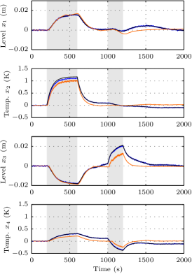
Figure 8: State trajectories for the thermo-fluid simulation example. Black: the actual states $x$; orange: event-based estimate $\hat{x}_{1}$ by Agent 1; blue: centralized estimate $\hat{x}_{\text{c}}$. The centralized estimate is shown for comparison and not available on any of the agents. The gray shaded areas indicate periods where step-wise process disturbances are active.

The average communication rates for event-based input and sensor transmissions are given in Fig. 9. Clearly, communication rates increase in the periods where the disturbances are active (gray areas), albeit not the same for all sensors and inputs. At times, when there is no disturbance, communication rates are very low in general. This highlights the intend behavior of event-based communication: sensor feedback only happens when necessary, in this case, when disturbances are active.

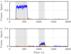
Figure 9: Event-based communication rates for the thermo-fluid simulation example: communication of level measurements $y_{1}$ and $y_{3}$ in black, for temperature measurements $y_{2}$ and $y_{4}$ in blue, and for the inputs $u_{1}$ and $u_{2}$ in orange. All rates are computed as the moving average over 100 steps.

Figure 10 shows the inter-agent error $e_{12}$; that is, the difference between the agents’ estimates. Jumps in the error signals are cause by a dropped packet. Clearly, the error decays after each impulse, which corresponds to the exponentially stable inter-agent dynamics (30) as per the previous discussion. Because of this, no synchronous resetting (31) is required in this example.

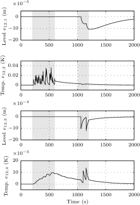
Figure 10: Inter-agent error $e_{12}$ for the thermo-fluid example. Jumps in error are caused by packet drops, decay afterward is due to stable inter-agent dynamics (30).

7 Concluding Remarks

Simplicity of design and implementation were key considerations when developing the approach for distributed and event-based state estimation herein. The proposed scheme emulates a centralized linear state observer design, and directly builds upon the typical periodic implementation of an observer-based control system. Starting from a centralized, periodic design (Section 2.2), only the event-triggers (13) and (24), and (for some problems) synchronous averaging (31) must be added. Observer and controller structure, as well as the transmitted quantities (measurements and inputs) remain unchanged, and no redesign of gains is necessary. The performance of the periodic design can be recovered by choosing small enough triggering thresholds, which greatly simplifies tuning in practice. Thus, implementation of the event-based scheme requires minimal extra effort, and virtually no additional design knowledge.

While conceptually straightforward, proving stability of the proposed architecture is non-trivial because the resulting observer dynamics are switching and coupled through process dynamics and communication. Together with the proposal of the architecture, establishing stability is the key contribution of this report. To prove stability for the general case, the synchronous averaging mechanism (31) was introduced. Yet, synchronous averaging can be avoided if the inter-agent dynamics (30) are stable (as in the example in Section 6.2). Currently ongoing work concerns synthesis approaches, where the observer gains are not taken from a centralized design, but designed for stable inter-agent dynamics.

The method proposed herein (albeit with full communication of inputs and without synchronous resetting), was successfully applied in (Trimpe, 2012) on the Balancing Cube test bed, i.e., a system with unstable dynamics. Comparable simulations of this system are presented herein.

References

- Akyildiz et al. [2002] I. Akyildiz, W. Su, Y. Sankarasubramaniam, and E. Cayirci. Wireless sensor networks: a survey. Computer Networks, 38(4):393–422, 2002.
- Åström and Wittenmark [1997] K. Åström and B. Wittenmark. Computer-controlled systems: theory and design. Prentice Hall, 1997.
- Battistelli et al. [2012] G. Battistelli, A. Benavoli, and L. Chisci. Data-driven communication for state estimation with sensor networks. Automatica, 48(5):926–935, 2012.
- Bernstein [2005] D. S. Bernstein. Matrix mathematics: theory, facts, and formulas with applications to linear system theory. Princeton University Press, Princeton, New Jersey, 2005.
- Böker and Lunze [2002] G. Böker and J. Lunze. Stability and performance of switching Kalman filters. International Journal of Control, 75(16/17):1269–1281, Nov. 2002.
- Callier and Desoer [1991] F. M. Callier and C. A. Desoer. Linear System Theory. Springer-Verlag, 1991.
- Cassandras [2014] C. G. Cassandras. The event-driven paradigm for control, communication and optimization. Journal of Control and Decision, 1(1):3–17, 2014.
- Delbrück et al. [2010] T. Delbrück, B. Linares-Barranco, E. Culurciello, and C. Posch. Activity-driven, event-based vision sensors. In IEEE International Symposium on Circuits and Systems, pages 2426–2429, 2010.
- Dimarogonas et al. [2012] D. Dimarogonas, E. Frazzoli, and K. Johansson. Distributed event-triggered control for multi-agent systems. IEEE Transactions on Automatic Control, 57(5):1291–1297, May 2012.
- Donkers and Heemels [2012] M. C. F. Donkers and W. P. M. H. Heemels. Output-based event-triggered control with guaranteed -gain and improved and decentralized event-triggering. IEEE Transactions on Automatic Control, 57(6):1362–1376, June 2012.
- Ferrari et al. [2012] F. Ferrari, M. Zimmerling, L. Mottola, and L. Thiele. Low-power wireless bus. In ACM Conference on Embedded Network Sensor Systems, pages 1–14, 2012.
- Grüne et al. [2014] L. Grüne, S. Hirche, O. Junge, P. Koltai, D. Lehmann, J. Lunze, A. Molin, R. Sailer, M. Sigurani, C. Stöcker, et al. Event-based control. In Control Theory of Digitally Networked Dynamic Systems, pages 169–261. Springer, 2014.
- Han et al. [2015] D. Han, Y. Mo, J. Wu, S. Weerakkody, B. Sinopoli, and L. Shi. Stochastic event-triggered sensor schedule for remote state estimation. IEEE Transactions on Automatic Control, 60(10):2661–2675, Oct. 2015.
- Heemels et al. [2012] W. P. M. H. Heemels, K. H. Johansson, and P. Tabuada. An introduction to event-triggered and self-triggered control. In IEEE Conference on Decision and Control, pages 3270–3285, 2012.
- Henningsson and Åström [2006] T. Henningsson and K. J. Åström. Log-concave observers. In International Symposium on Mathematical Theory of Networks and Systems, July 2006.
- Hespanha et al. [2007] J. P. Hespanha, P. Naghshtabrizi, and Y. Xu. A survey of recent results in networked control systems. Proceedings of the IEEE, 95(1):138–162, Jan. 2007.
- Imer and Basar [2005] O. Imer and T. Basar. Optimal estimation with limited measurements. In IEEE Conference on Decision and Control, pages 1029–1034, Dec. 2005.
- Kim and Kumar [2012] K.-D. Kim and P. Kumar. Cyber-physical systems: A perspective at the centennial. Proceedings of the IEEE, 100(Special Centennial Issue):1287–1308, May 2012.
- Lemmon [2010] M. Lemmon. Event-triggered feedback in control, estimation, and optimization. In Networked Control Systems, pages 293–358. Springer, 2010.
- Liu et al. [2015] Q. Liu, Z. Wang, X. He, and D. Zhou. Event-based recursive distributed filtering over wireless sensor networks. IEEE Transactions on Automatic Control, 60(9):2470–2475, Sept. 2015.
- Lunze and Lehmann [2010] J. Lunze and D. Lehmann. A state-feedback approach to event-based control. Automatica, 46(1):211–215, 2010.
- Marck and Sijs [2010] J. Marck and J. Sijs. Relevant sampling applied to event-based state-estimation. In Int. Conf. on Sensor Technologies and Applications, pages 618–624, July 2010.
- Mazo Jr and Tabuada [2008] M. Mazo Jr and P. Tabuada. On event-triggered and self-triggered control over sensor/actuator networks. In IEEE Conference on Decision and Control, pages 435–440, 2008.
- Mazo Jr and Tabuada [2011] M. Mazo Jr and P. Tabuada. Decentralized event-triggered control over wireless sensor/actuator networks. IEEE Transactions on Automatic Control, 56(10):2456–2461, 2011.
- Mignone et al. [2000] D. Mignone, G. Ferrari-Trecate, and M. Morari. Stability and stabilization of piecewise affine and hybrid systems: an LMI approach. In IEEE Conference on Decision and Control, pages 504–509, 2000.
- Miskowicz [2006] M. Miskowicz. Send-on-delta concept: an event-based data reporting strategy. Sensors, 6(1):49–63, 2006.
- Molin and Hirche [2014] A. Molin and S. Hirche. A bi-level approach for the design of event-triggered control systems over a shared network. Discrete Event Dynamic Systems, 24(2):153–171, 2014.
- Muehlebach and Trimpe [2015] M. Muehlebach and S. Trimpe. LMI-based synthesis for distributed event-based state estimation. In American Control Conference, 2015.
- Persis et al. [2013] C. D. Persis, R. Sailer, and F. Wirth. Parsimonious event-triggered distributed control: A zeno free approach. Automatica, 49(7):2116–2124, 2013.
- Rabi et al. [2006] M. Rabi, G. Moustakides, and J. Baras. Multiple sampling for estimation on a finite horizon. In IEEE Conference on Decision and Control, pages 1351–1357, Dec. 2006.
- Shi et al. [2014] D. Shi, T. Chen, and L. Shi. An event-triggered approach to state estimation with multiple point- and set-valued measurements. Automatica, 50(6):1641 – 1648, 2014.
- Sigurani et al. [2015] M. Sigurani, C. Stöcker, L. Grüne, and J. Lunze. Experimental evaluation of two complementary decentralized event-based control methods. Control Engineering Practice, 35:22–34, 2015.
- Sijs and Lazar [2012] J. Sijs and M. Lazar. Event based state estimation with time synchronous updates. IEEE Transactions on Automatic Control, 57(10):2650–2655, Oct. 2012.
- Sijs et al. [2013] J. Sijs, B. Noack, and U. Hanebeck. Event-based state estimation with negative information. In Int. Conf. on Information Fusion, pages 2192–2199, July 2013.
- Sijs et al. [2014] J. Sijs, L. Kester, and B. Noack. A study on event triggering criteria for estimation. In Int. Conf. on Information Fusion, pages 1–8, July 2014.
- Stöcker et al. [2013] C. Stöcker, D. Vey, and J. Lunze. Decentralized event-based control: Stability analysis and experimental evaluation. Nonlinear Analysis: Hybrid Systems, 10:141–155, Nov. 2013.
- Tallapragada and Chopra [2014] P. Tallapragada and N. Chopra. Decentralized event-triggering for control of nonlinear systems. IEEE Transactions on Automatic Control, 59(12):3312–3324, 2014.
- Thomesse [2005] J.-P. Thomesse. Fieldbus technology in industrial automation. Proceedings of the IEEE, 93(6):1073–1101, 2005.
- Trimpe [2012] S. Trimpe. Event-based state estimation with switching static-gain observers. In IFAC Workshop on Distributed Estimation and Control in Networked Systems, pages 91–96, Sept. 2012.
- Trimpe [2014] S. Trimpe. Stability analysis of distributed event-based state estimation. In IEEE Conference on Decision and Control, pages 2013–2019, Dec. 2014.
- Trimpe and Campi [2015] S. Trimpe and M. Campi. On the choice of the event trigger in event-based estimation. In Int. Conf. on Event-based Control, Communication, and Signal Processing, 2015.
- Trimpe and D’Andrea [2011a] S. Trimpe and R. D’Andrea. An experimental demonstration of a distributed and event-based state estimation algorithm. In IFAC World Congress, pages 8811–8818, 2011a.
- Trimpe and D’Andrea [2011b] S. Trimpe and R. D’Andrea. Reduced communication state estimation for control of an unstable networked control system. In IEEE Conference on Decision and Control, pages 2361–2368, 2011b.
- Trimpe and D’Andrea [2012a] S. Trimpe and R. D’Andrea. The Balancing Cube: A dynamic sculpture as test bed for distributed estimation and control. IEEE Control Systems Magazine, 32(6):48–75, Dec. 2012a.
- Trimpe and D’Andrea [2012b] S. Trimpe and R. D’Andrea. Numerical models and controller design parameters for the Balancing Cube. Technical report, ETH Zurich, 2012b. URL http://dx.doi.org/10.3929/ethz-a-007343301.
- Trimpe and D’Andrea [2014] S. Trimpe and R. D’Andrea. Event-based state estimation with variance-based triggering. IEEE Transaction on Automatic Control, 59(12):3266–3281, Dec. 2014.
- Tsividis [2010] Y. Tsividis. Event-driven data acquisition and digital signal processing: a tutorial. IEEE Transactions on Circuits and Systems II: Express Briefs, 57(8):577–581, 2010.
- Wang and Lemmon [2008] X. Wang and M. Lemmon. Decentralized event-triggered broadcasts over networked control systems. In Hybrid Systems: Computation and Control, pages 674–677. Springer, 2008.
- Wang and Lemmon [2011] X. Wang and M. Lemmon. Event-triggering in distributed networked control systems. IEEE Transactions on Automatic Control, 56(3):586–601, Mar. 2011.
- Weimer et al. [2012] J. Weimer, J. Araujo, and K. H. Johansson. Distributed event-triggered estimation in networked systems. In IFAC Conf. on Analysis and Design of Hybrid Systems, pages 178–185, June 2012.
- Wu et al. [2013] J. Wu, Q.-S. Jia, K. Johansson, and L. Shi. Event-based sensor data scheduling: Trade-off between communication rate and estimation quality. IEEE Transactions on Automatic Control, 58(4):1041–1046, Apr. 2013.
- Xu and Hespanha [2004] Y. Xu and J. Hespanha. Optimal communication logics in networked control systems. In IEEE Conference on Decision and Control, pages 3527–3532, Dec. 2004.
- Yan et al. [2014] L. Yan, X. Zhang, Z. Zhang, and Y. Yang. Distributed state estimation in sensor networks with event-triggered communication. Nonlinear Dynamics, 76:169–181, 2014.
- Yook et al. [2002] J. K. Yook, D. M. Tilbury, and N. R. Soparkar. Trading computation for bandwidth: reducing communication in distributed control systems using state estimators. IEEE Transactions on Control Systems Technology, 10(4):503–518, July 2002.