Thermodynamics and reference scale of SU(3) gauge theory from gradient flow on fine lattices

Abstract:

We study the parametrization of lattice spacing and thermodynamics of SU(3) gauge theory on the basis of the Yang-Mills gradient flow on fine lattices. The lattice spacing of the Wilson gauge action is determined over a wide range $6.3\leq\beta\leq 7.5$ with high accuracy. The measurements of the flow time and lattice spacing dependences of the expectation values of the energy-momentum tensor are performed on fine lattices.

1 Introduction

After the introduction of the Yang-Mills gradient flow in lattice gauge theory [1], this concept has been successfully applied to various purposes in lattice QCD numerical simulations [2, 3]. In this proceedings, we report our recent studies on the application of the gradient flow for two purposes.

In the first analysis, we measure the lattice spacing of the SU(3) Wilson gauge action [4]. We introduce reference scales having physical dimension on the basis of the gradient flow [1, 5], and perform the measurement of lattice spacing in this scale in the range $6.3\leq\beta=6/g^{2}\leq 7.5$. We use the reference scale called $w_{0.4}$ in this analysis. The parametrization of the lattice spacing as a function of $\beta$ is given in Eq. (7). The relation between $w_{0.4}$ and other reference scales, as well as the finite volume and lattice discretization effects in our analysis are also discussed [4].

Secondly, we apply the gradient flow for the measurement of thermodynamics of SU(3) gauge theory. In this analysis, we use the energy-momentum tensor (EMT) operator defined by the gradient flow [6] with the small flow-time expansion [7]. The thermodynamic quantities are obtained by taking the expectation values of the EMT operator. In Ref. [8], we performed the measurement of the thermodynamics of SU(3) gauge theory, and found that this method can successfully analyze the thermodynamics with good statistics compared with the previously-known integral method. In this proceedings we report the update of this analysis on finer lattices with temporal lattice size $N_{t}=12$–$32$.

2 Gradient flow

Let us first give a brief review on the gradient flow. The gradient flow for the Yang-Mills gauge field is the continuous transformation of the field defined by the differential equation [1]

$$\frac{dA_{\mu}}{dt}=-g_{0}^{2}\frac{\partial S_{\rm YM}(t)}{\partial A_{\mu}}=D_{\nu}G_{\nu\mu},$$ (1)

with the Yang-Mills action $S_{\rm YM}(t)$ composed of $A_{\mu}(t)$. Color indices are suppressed for simplicity. The initial condition at $t=0$ is taken for the field in the conventional gauge theory; $A_{\mu}(0)=A_{\mu}$. The flow time $t$, which has a dimension of inverse mass squared, is a parameter which controls the transformation. The gauge field is transformed along the steepest descent direction as $t$ increases. At the tree level, Eq. (1) is rewritten as

$$\frac{dA_{\mu}}{dt}=\partial_{\nu}\partial_{\nu}A_{\mu}+{\rm(gauge~{}dependent~{}terms)}.$$ (2)

Neglecting the gauge dependent terms, Eq. (2) is the diffusion equation in four-dimensional space. For positive $t$, therefore, the gradient flow acts as the cooling of the gauge field with the smearing radius $\sqrt{8t}$.

In Ref. [7], it is rigorously proved that all composite operators composed of $A_{\mu}(t)$ take finite values for $t>0$. This property ensures that observables at $t>0$ are regularization independent. In the present study, we use the gradient flow for two purposes; (1) the introduction of reference scales and the measurement of lattice spacing [1], and (2) the measurement of thermodynamic observables [8] using the energy-momentum tensor operator defined by the gradient flow with the small flow-time expansion [6].

In the present study we consider two observables,

$$E(t) =\frac{1}{4}G_{\mu\nu}^{a}(t)G_{\mu\nu}^{a}(t),$$ (3)

$$U_{\mu\nu}(t,x) =G_{\mu\rho}^{a}(t,x)G_{\nu\rho}^{a}(t,x)-\frac{1}{4}\delta_{\mu\nu}G_{\rho\sigma}^{a}(t,x)G_{\rho\sigma}^{a}(t,x),$$ (4)

at positive flow time $t>0$, where $G_{\mu\nu}^{a}(t)$ is the “field strength” composed of $A_{\mu}(t)$.

3 Reference scale and lattice spacing

In this section, we analyze the lattice spacing of SU(3) Wilson gauge action [4]. In order to define reference scales and measure lattice spacing with the gradient flow, we use an observation that the expectation value of an observable at $t>0$ is regularization independent [1]. From this property, the expectation value of dimensionless observables does not depend on regularization. On the lattice, therefore, they should be the lattice spacing, $a$, independent up to $O(a^{2})$ effects. By choosing $t^{2}E(t)$ as the dimensionless observable, the value of $t$ at which $t^{2}\langle E(t)\rangle$ takes a specific value $X$, i.e. the solution of the equation

$$\left.t^{2}\langle E(t)\rangle\right|_{t=t_{{}_{X}}}=X,$$ (5)

is a dimensionful quantity, which can be used as a reference scale to introduce physical unit in lattice gauge theory. In Ref. [1], $t_{{}_{X}=0.3}$ (sometimes called $t_{0}$) is used as the reference scale. In Ref. [5], a quantity $w_{{}_{X}}$ defined by

$$\left.t\frac{d}{dt}t^{2}\langle E(t)\rangle\right|_{t=w_{{}_{X}}^{2}}=X,$$ (6)

is proposed as an alternative reference scale. In Ref. [5], a reference scale $w_{{}_{X}=0.3}$ (sometimes called $w_{0}$) is employed to set the scale.

In the present study we consider reference scales, $t_{{}_{X}}$ and $w_{{}_{X}}$ with $X=0.2$, $0.3$ and $0.4$. Larger $X$ is preferable to suppress the lattice discretization error, while the smearing radius $\sqrt{8t}$ would eventually hit the lattice boundary for too large $X$. We use $w_{0.4}$ and $w_{0.2}$ for the reference scales and introduce a new parametrization of the lattice spacing $a$ in terms of the bare coupling $\beta=6/g_{0}^{2}$ by a hybrid use of these reference scales. In this method, we measure the lattice spacing in the range $6.3<\beta<7.5$.

$\beta$	6.3	6.4	6.5	6.6	6.7	6.8	6.9	7.0	7.2	7.4	7.5
$N_{\rm s}$	64	64	64	64	64	64	64	96	96	128	128
$N_{\rm conf}$	30	100	49	100	30	100	30	60	53	40	60

Table 1: Simulation parameters $\beta=6/g_{0}^{2}$, the lattice size $N_{\rm s}$ and the number of configurations $N_{\mathrm{conf}}$ [4].

We perform numerical analyses of the SU(3) Yang–Mills theory with the Wilson plaquette action with the periodic boundary condition with the lattice size $N_{\rm s}^{4}$. The values of $\beta=6/g_{0}^{2}$, $N_{\rm s}$ and the number of configurations $N_{\mathrm{conf}}$ are summarized in Table 1. For $\beta=7.0$, $7.2$ and $7.4$, we have performed another measurements with different spatial sizes; $N_{\rm s}=64$, $64$ and $96$, for $\beta=7.0$, $7.2$ and $7.4$, respectively. From the comparison of the numerical results with different $N_{\rm s}$, we have checked that the finite volume effects are well suppressed with the choices of $N_{\rm s}$ shown in Table 1 [4].

We use the Wilson gauge action $S_{\mathrm{YM}}$ for the flow equation in Eq. (1). To construct the operator $E$, we use the clover-type representation of $G_{\mu\nu}^{a}$ unless otherwise stated. The numerical error of the Runge–Kutta (RK) method to solve the differential equation Eq. (1) have been estimated by comparing the numerical results with different integration step sizes. We have checked that the numerical error of the RK method is within two orders in magnitude smaller than the statistical errors.

Autocorrelation between different configurations is analyzed by the autocorrelation function and the dependence of the jackknife statistical errors against the bin-size, $N_{\mathrm{bin}}$. These analyses show that the autocorrelation is not visible within statistics in our set of gauge configurations, which are separated by $1,000$ Monte-Carlo steps composed of heatbath and five over-relaxation updates. On the other hand, the autocorrelation of the topological charge is known to become longer as the lattice spacing becomes finer due to the critical slowing down [1]. It is desirable to perform new measurements of the topological charge to investigate the effect of the critical slowing down on our analysis, which is left for our future work.

As pointed out in Ref. [5], the discretization error of $w_{0.3}$ is smaller than $t_{0.3}$. We thus employ $w_{{}_{X}}$ as the key reference scale in this paper. We also note that the lattice artifact is expected to be smaller for larger $X$. To check the discretization effects, we compare $t^{2}\langle E(t)\rangle$ and $t\frac{d}{dt}t^{2}\langle E(t)\rangle$ defined from the clover-type representation with those defined from $E(t)=2(1-P(t))$ using the average plaquette $P(t)$ [4]. This analysis shows that the difference between the two definitions is suppressed for large $t$. Moreover, the difference is more suppressed in $t\frac{d}{dt}t^{2}\langle E(t)\rangle$ than that in $t^{2}\langle E(t)\rangle$, i.e. the discretization effect in the former is smaller than the latter. We thus employ $w_{0.4}$ as the key reference scale. In our simulations, we estimate $w_{0.4}/a$ for $\beta=7.4$, $7.5$ using the data at small flow time ($w_{0.2}/a$) for these $\beta$ and the extrapolation of the ratio $w_{0.4}/w_{0.2}=1.3042(9)$ to the continuum limit [4].

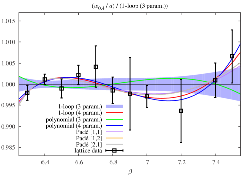
Figure 1: Result of the three parameter fit of $w_{0.4}/a$ given in Eq. (3.3) [4]. Squares are the data obtained by the numerical analyses normalized by Eq. (3.3). Shaded band indicates the uncertainty originating from the errors of the fitted coefficients. Results with several other fitting functions normalized by Eq. (3.3) are also plotted as well; see, Ref. [4].

For practical applications, it is convenient to introduce a parametrization of the ratio $w_{0.4}/a$ in terms of $\beta$. We have carried out such parametrization using various types of fitting functions. Among them, the three parameter fit motivated by the one-loop perturbation theory provides a reasonable result ($\chi^{2}/{\mathrm{dof}}=0.917$) for $11$ data points in $6.3\leq\beta\leq 7.5$ without over fitting:

$$\frac{w_{0.4}}{a}=\exp\left(\frac{4\pi^{2}}{33}\beta-8.6853+\frac{37.422}{\beta}-\frac{143.84}{\beta^{2}}\right)[1\pm 0.004(\mathrm{stat.})\pm 0.007(\mathrm{sys.})].$$ (7)

In Fig. 1, we show the numerical results of $w_{0.4}/a$ normalized by the fitting function Eq. (7). The shaded band in Fig. 1 is the error associated with the fitting parameters in Eq. (7). The results of some other fitting functions normalized by Eq. (7) are also plotted in Fig. 1 [4]. They agree with each other within $0.5\%$ in the range, $6.3\leq\beta\leq 7.5$.

We have checked that our parametrization agrees with the previously known ones in the range of $\beta$ at which both parametrizations are applicable within the error [4]. In Ref. [4], we have also determined the relation between $w_{0.4}$ and other reference scales, such as $t_{0}=t_{0.3}$, $w_{0}=w_{0.3}$, the Sommer scale $r_{0}$, lambda parameter and critical temperature.

4 Thermodynamics

Next, we report on the update of the measurement of thermodynamics performed in Refs. [8, 9]. In this analysis, we use the energy-momentum tensor (EMT) defined by the small flow time expansion [7, 6]. This expansion asserts that a composite operator $\tilde{O}(t,x)$ at positive flow time in the $t\to 0$ limit can be written by a superposition of operators of the original gauge theory at $t=0$ as

$$\tilde{O}(t,x)\xrightarrow[t\to 0]{}\sum_{i}c_{i}(t)O_{i}^{\rm R}(x),$$ (8)

where $O_{i}^{\rm R}(x)$ on the right-hand side represents renormalized operators in some regularization scheme in the original gauge theory at $t=0$ with the subscript $i$ denoting different operators, and $x$ represents the coordinate in four-dimensional space-time. Similarly to the Wilson coefficients in the operator product expansion (OPE), the coefficients $c_{i}(t)$ in Eq. (8) can be calculated perturbatively [7].

Using Eq. (8), one can define the renormalized EMT [6]. For this purpose, we first consider the operators defined in Eqs. (3) and (4), which are dimension-four gauge-invariant operators, as the left-hand side in Eq. (8). Although these operators are quite similar to the trace and traceless-part of the EMT, they are not the EMT since $G_{\mu\nu}(t,x)$ is defined at nonzero flow time $t>0$. Because these operators are gauge invariant, when they are expanded as in Eq. (8) only gauge invariant operators can appear in the right-hand side. Such operator with the lowest dimension is an identity operator. In the expansion of the traceless operator Eq. (4), however, the constant term cannot appear. The next gauge-invariant operators are the dimension-four EMTs. Up to this order, therefore, the small flow time expansions of Eqs. (4) and (3) are given by

$$U_{\mu\nu}(t,x) =\alpha_{U}(t)\left[T_{\mu\nu}^{R}(x)-\frac{1}{4}\delta_{\mu\nu}T_{\rho\rho}^{R}(x)\right]+O(t),$$ (9)

$$E(t,x) =\left\langle E(t,x)\right\rangle_{0}+\alpha_{E}(t)T_{\rho\rho}^{R}(x)+O(t),$$ (10)

where $\langle\cdot\rangle_{0}$ is vacuum expectation value and $T_{\mu\nu}^{R}(x)$ is the correctly normalized conserved EMT with its vacuum expectation value subtracted. Abbreviated are the contributions from the operators of dimension $6$ or higher, which are proportional to powers of $t$ because of dimensional reasons, and thus suppressed for small $t$.

Combining relations Eqs. (9) and (10), we have

$$T_{\mu\nu}^{R}(x)=\lim_{t\to 0}\left\{\frac{1}{\alpha_{U}(t)}U_{\mu\nu}(t,x)+\frac{\delta_{\mu\nu}}{4\alpha_{E}(t)}\left[E(t,x)-\left\langle E(t,x)\right\rangle_{0}\right]\right\}.$$ (11)

The coefficients $\alpha_{U}(t)$ and $\alpha_{E}(t)$ are calculated perturbatively up to next to leading order in Ref. [6]. Using Eq. (11), the energy density $e$ and pressure $p$ are obtained by taking the expectation values of diagonal components as

$$e=\langle T_{00}\rangle,\quad p=\frac{1}{3}\langle T_{11}+T_{22}+T_{33}\rangle.$$ (12)

$N_{t}$	12	16	20	24	32
$\beta$	6.719	6.941	7.117	7.256	7.500

Table 2: The simulation parameter for the measurement of thermodynamics at $T=1.66T_{c}$.

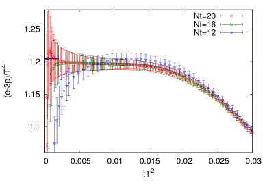
Figure 2: Flow time dependence of the dimensionless interaction measure $(e-3p)/T^{4}$ (left panel) and the dimensionless entropy density $(e+p)/T^{4}$ (right panel) for different lattice spacings at $T/T_{c}=1.66$. The continuum extrapolated result obtained in the integral method in Ref. [10] is indicated by the arrow at vertical axis.

In the following, we present our numerical results on the thermodynamics with $N_{t}=12$ – $32$ for $T=1.66T_{c}$ of SU(3) gauge theory with Wilson gauge action. The values of $\beta$ for different temporal lattice length $N_{t}$ are determined using Eq. (7). These values are shown in Table 2. All lattices have the aspect ratio $N_{s}/N_{t}$ larger than $5.3$. We use the Wilson gauge action $S_{\mathrm{YM}}$ for the flow equation in Eq. (1). The operators $E$ and $U$ on the lattice are constructed from the clover-type representation of $G_{\mu\nu}^{a}$.

In Fig. 2, we show the numerical results for the dimensionless trace anomaly $\Delta/T^{4}=(e-3p)/T^{4}$ and the dimensionless entropy density $s/T^{3}=(e+p)/T^{4}$ at $T=1.66T_{c}$ as functions of the flow parameter $tT^{2}$. The figure shows that these functions have a linear behavior in the moderate values of $tT^{2}$. The numerical results show deviation from this trend for small and large $t$. The deviation at small $t$ in the range $\sqrt{8t}\lesssim 2a$ is attributed to the lattice discretization effects. On the other hand, the decrease at large $t$ in the range $\sqrt{8t}\gtrsim 1/(2T)$ is understood as the oversmearing; the smearing by the gradient flow exceeds the temporal lattice size in this range [8]. In both panels in Fig. 2, we show the continuum-extrapolated values of $\Delta/T^{4}$ and $s/T^{3}$ with the same temperature obtained by the integral method [10] by the blue arrow beside the $y$ axis. The figure shows that the $y$-intercepts of the linear behavior of our results well agree with this result. To extract the physical values of $\Delta/T^{4}$ and $s/T^{3}$ in our method, we have to take the double limit $(a,t)\to(0,0)$ from the range satisfying $\sqrt{8t_{\rm min}}\gg 2a$. This analysis will be reported in the future publication.

The measurement of thermodynamic quantities using gradient flow is also applicable to full QCD [11]. A first numerical analysis is reported in Ref. [12].

Numerical simulation for this study was carried out on IBM System Blue Gene Solution at KEK under its Large-Scale Simulation Program (Nos. T12-04, 13/14-20 and 14/15-08). The work of M. A., M. K., and H. S. are supported in part by a Grant-in-Aid for Scientific Researches 23540307 and 26400272, 25800148 and 23540330,respectively. E. I. is supported in part by Strategic Programs for Innovative Research (SPIRE) Field 5. T. H. is partially supported by RIKEN iTHES Project.

References

- [1] M. Lüscher, JHEP 1008, 071 (2010) [arXiv:1006.4518 [hep-lat]].
- [2] Reviewed in, M. Lüscher, PoS LATTICE 2013, 016 (2014) [arXiv:1308.5598 [hep-lat]].
- [3] A. Ramos, PoS LATTICE 2014, 017 (2015) [arXiv:1506.00118 [hep-lat]].
- [4] M. Asakawa, T. Iritani, M. Kitazawa and H. Suzuki, arXiv:1503.06516 [hep-lat].
- [5] S. Borsanyi, et al., JHEP 1209, 010 (2012) [arXiv:1203.4469 [hep-lat]].
- [6] H. Suzuki, PTEP 2013, 083B03 (2013) [erratum PTEP 2015, 079201 (2015)] [arXiv:1304.0533 [hep-lat]].
- [7] M. Lüscher and P. Weisz, JHEP 1102, 051 (2011) [arXiv:1101.0963 [hep-th]].
- [8] M. Asakawa, et al. [FlowQCD Collaboration], Phys. Rev. D 90, no. 1, 011501 (2014) [erratum Phys. Rev. D 92, no. 5, 059902 (2015)] [arXiv:1312.7492 [hep-lat]].
- [9] M. Kitazawa, et al. PoS LATTICE 2014, 022 (2014) [arXiv:1412.4508 [hep-lat]].
- [10] S. Borsanyi, et al. JHEP 1207, 056 (2012) [arXiv:1204.6184 [hep-lat]].
- [11] H. Makino and H. Suzuki, PTEP 2014, no. 6, 063B02 (2014) [arXiv:1403.4772 [hep-lat]].
- [12] E. Itou, et al. PoS, LATTICE 2015, 303 (2015) [arXiv:1511.03009 [hep-lat]].