On the dependence of the type Ia SNe luminosities
on the metallicity of their host galaxies

Abstract

The metallicity of the progenitor system producing a type Ia supernova (SN Ia) could play a role in its maximum luminosity, as suggested by theoretical predictions. We present an observational study to investigate if such a relationship there exists. Using the 4.2m WHT we have obtained intermediate-resolution spectroscopy data of a sample of 28 local galaxies hosting SNe Ia, for which distances have been derived using methods independent to those based on the own SN Ia parameters. From the emission lines observed in their optical spectrum, we derived the gas-phase oxygen abundance in the region where each SN Ia exploded. Our data show a trend, with a 80% of chance not to be due to random fluctuation, between SNe Ia absolute magnitudes and the oxygen abundances of the host galaxies, in the sense that luminosities tend to be higher for galaxies with lower metallicities. This result seems like to be in agreement with both the theoretically expected behavior, and with other observational results. This dependence $M_{B}$-Z might induce to systematic errors when is not considered in deriving SNe Ia luminosities and then using them to derive cosmological distances.

1 INTRODUCTION

The Supernova Cosmology is based on the well-known Hubble Diagram (HD) in which distances of SNe Ia are represented as a function of their redshifts, $z$, usually determined with high accuracy from SNe Ia or host galaxies spectra. Distances are derived by means of the distance modulus, $\mu=m-M$. Phillips (1993); Hamuy et al. (1996a, b), and Phillips et al. (1999) found a correlation between the properties of the SN Ia light curve (LC) and the absolute magnitude in its maximum for $B$, $V$ and $I$ bands. Therefore, under the assumption that SNe Ia are standard-calibrated candles, their absolute magnitude $M$ can be obtained from empirical calibrations based on their observed LCs. Thus, the SNe Ia-based cosmology projects discovered the Universe is in accelerated expansion (Perlmutter et al., 1999; Riess et al., 1998).

However, the SNe Ia methodology is calibrated on local objects, whose host galaxies probably share almost solar abundances. But chemical abundances change with redshift (e.g. Lara-López et al., 2009, and references therein) due to chemical evolution of galaxies, therefore the LC calibration might not be the same for chemical abundances which differ very much from solar values. This possible metallicity dependence of the SNe Ia luminosity has been neglected but it might play a role in accurately determining the distances to cosmological SNe Ia. Since the number of SNe Ia detections will extraordinarily increase in the forthcoming surveys (DES, LSST), statistical errors will decrease while systematic errors will begin to dominate, limiting the precision of SNe Ia as indicators of extragalactic distances. The metallicity dependence may be one source of systematic errors when using these techniques, being therefore important to quantify its effect.

A dependence of the maximum luminosity of SNe Ia on the initial metallicity of their progenitors is theoretically predicted. SNe Ia are thought to be thermonuclear explosions of carbon-oxygen white dwarfs (WD) in binary systems, (Whelan & Iben, 1973; Iben & Tutukov, 1984; Webbink, 1984). The WD approaches the critical Chandrasekhar mass by accretion from its companion. The maximum luminosity of a SN Ia depends on the amount of ⁵⁶Ni synthesized during the explosion (Arnett et al., 1982):

$$L\propto M(^{56}\rm Ni)~{}~{}erg\,s^{-1},$$ (1)

Assuming the mass of the exploding WD is constant, the parameter who leads the relation between the LC parameters and its maximum magnitude is the outer layer opacity of the ejected material (Hoeflich & Khokhlov, 1996), which depends on temperature and, thus, on the heating due to the radioactive $\rm{}^{56}Ni$ decay. The neutron excess in the exploding WD, which controls the radioactive ($\rm{}^{56}Ni$) to non-radioactive (Fe-peak elements) abundance ratio, depends directly on the initial metallicity of the progenitor. Therefore the maximum luminosity of the SN Ia explosion depends on the initial abundances of C, N, O, and Fe of the WD progenitor (Timmes, Brown, & Truran, 2003; Travaglio, Hillebrandt, & Reinecke, 2005; Podsiadlowski et al., 2006). Timmes, Brown, & Truran (2003) found a dependence on Z as $1-0.057{\rm Z/Z_{\sun}}$. Bravo et al. (2010) computed a series of SNe Ia explosions, finding a stronger dependence on Z:

$$M(^{56}{\rm Ni})\sim f({\rm Z})=1-0.075\frac{\rm Z}{\rm Z_{\odot}}$$ (2)

They also explored the dependence of the explosion on the local chemical composition, finding a non-linear relation :

$$M(^{56}Ni)\sim f({\rm Z})=1-0.18\frac{\rm Z}{\rm Z_{\odot}}\Bigg{(}1-0.10\frac{\rm Z}{\rm Z_{\odot}}\Bigg{)}$$ (3)

Since the luminosity decreases with Z increasing, SNe Ia located in galaxies with $\rm Z>Z_{\odot}$ might be dimmer than expected as compared to those with $\rm Z\leq Z_{\odot}$

The dependence of SNe Ia luminosities on the metallicity was studied by Gallagher et al. (2005), who estimated oxygen elemental abundances by using host-galaxies emission lines, finding most metal-rich galaxies have the faintest SNe Ia. They based their conclusion on the analysis of the HD residuals, implying they used SNe Ia to extract the magnitudes. Gallagher et al. (2008) analyzed spectral absorption indices in early-type galaxies, using theoretical evolutive synthesis models (still not very precise, Sánchez et al. in prep.), also finding a trend between SNe Ia magnitudes and the metallicity of their stellar populations. These results are in agreement with theoretical predictions.

Other dependences of SNe Ia magnitudes have been found studying the correlations between the residuals in the HD, as $\mu-\mu_{fit}$, and the host galaxy characteristics. SNe Ia in massive galaxies result brighter than spected after correcting for their LC widths and colors (see Howell et al., 2009; Neill et al., 2009; Sullivan et al., 2010; Lampeitl et al., 2010; Childress et al., 2013; Pan et al., 2014; Betoule et al., 2014; Moreno-Raya et al., 2015, and references therein for more details). Dividing the galaxy mass range into two groups, the $M_{B}$ of SNe Ia shows a step of $\sim$ 0.07-0.10 mag dex^-1 in the residuals plot (see Childress et al., 2013, mainly Table 2, where observational trends from different authors are compiled) between both bins.

Following Rigault et al. (2013) and Galbany et al. (2014), our aim is to perform a systematic study to determine if SNe Ia luminosities depend on the local elemental abundances of their host galaxies. We built a sample of nearby galaxies hosting SNe Ia, selecting objects for which distances were determined using methods different to those based on SN Ia. We then conducted intermediate-resolution long-slit spectroscopic observations of the sample to estimate the oxygen gas-phase abundances and, when possible, derive the local metallicity around the region where SNe Ia exploded. With that we directly check the possible luminosity-metallicity relationship.

2 OBSERVATIONS AND OXYGEN ABUNDANCES

We have observations for 28 local galaxies hosting SNe Ia with the 4.2m William Herschel Telescope (WHT) at El Roque de Los Muchachos Observatory, La Palma, Spain, in two campaigns in December 2011 (9 galaxies) and January 2014 (19 galaxies). We observed more galaxies but they did not show emission lines with sufficient S/N ratio to measure their intensities. Therefore by construction, our sample is biased to star-forming galaxies. We used the two arms of the ISIS spectrograph, covering from 3600 to 5200 Å in the blue and from 5850 to 7900 Å in the red, with 0.45 Å/pix and 0.49 Å/pix, respectively. Galaxies were chosen from Neill et al. (2009), selecting objects not in the Hubble flow ($z\leq 0.02$) and for which distances not based on SNe Ia data are available. Table 1 compiles the details of the observed sample. 89 H ii regions were analyzed. We have many galaxies with oxygen abundances estimates for several regions, for which we determined a metallicity radial gradient (Moreno-Raya et al., 2015).

Table 1: Sample of observed galaxies and their associated SNe Ia. Galaxy names in column 1, galaxy center coordinates RA and DEC in columns 2 and 3, and hosted SNe Ia in column 4, host galaxies magnitudes, $M_{B}$, in column 5, and the corresponding redshift $z$ in column 6. Distance indicator and SN Ia class, as reddened (R) , normal (N) or subluminous (S), are shown in columns 7 and 8., and LC fitters in column 9.

Object	RA	DEC	SN Ia	$\rm M_{B}$	$z$	Distance indicator∗	SN Ia class	LC fitter
MGC 021602	06 04 34.9	-12 37 29	2003kf	-19.86	0.007388	TF	N	SALT2
NGC 0105	00 25 16.6	+12 53 22	1997cw	-20.98	0.017646	SN Ia	R	SALT2
NGC 1275	03 19 48.1	+41 30 42	2005mz	-22.65	0.017559	TF	S	SALT2
NGC 1309	03 22 06.5	-15 24 00	2002fk	-20.57	0.007125	CEPH & TF	N	SALT2
NGC 2935	09 36 44.8	-21 07 41	1996Z	-20.69	0.007575	TF	R	SALT2
NGC 3021	09 50 57.1	+33 33 13	1995al	-19.86	0.005140	CEPH & TF	N	SALT2
M 82	09 55 52.7	+69 40 46	2014J	-20.13	0.000677	PNLF	N	—–
NGC 3147	10 16 53.6	+73 24 03	1997bq	-22.22	0.009346	TF	N	SALT2
NGC 3169	10 14 15.0	+03 27 58	2003cg	-20.42	0.004130	TF	R	SALT2
NGC 3368	10 46 45.7	+11 49 12	1998bu	-20.96	0.002992	CEPH & TF	R	MLCS2k2
NGC 3370	10 47 04.0	+17 16 25	1994ae	-19.77	0.004266	CEPH & TF	N	MLCS2k2
NGC 3672	11 25 02.5	-09 47 43	2007bm	-20.63	0.006211	TF	R	SALT2
NGC 3982	11 56 28.1	+55 07 31	1998aq	-19.91	0.003699	CEPH & TF	N	MLCS2k2
NGC 4321	12 22 54.8	+15 49 19	2006X	-22.13	0.005240	CEPH & TF	R	SALT2
NGC 4501	12 31 59.1	+14 25 13	1999cl	-23.13	0.007609	TF	R	SALT2
NGC 4527	12 34 08.4	+02 39 13	1991T	-21.55	0.005791	CEPH & TF	N	MLCS2k2
NGC 4536	12 34 27.0	+02 11 17	1981B	-21.85	0.006031	CEPH & TF	N	MLCS2k2
NGC 4639	12 42 52.4	+13 15 27	1990N	-19.24	0.003395	CEPH & TF	N	MLCS2k2
NGC 5005	13 10 56.2	+37 03 33	1996ai	-21.48	0.003156	TF	R	SALT2
NGC 5468	14 06 34.9	-05 27 11	1999cp	-20.33	0.009480	TF	N	SALT2
NGC 5584	14 22 23.8	-00 23 16	2007af	-19.69	0.005464	CEPH & TF	N	SALT2
UGC 272	00 27 49.7	-01 12 00	2005hk	-19.42	0.012993	TF	S	MLCS2k2
UGC 3218	05 00 43.7	+62 14 39	2006le	-22.17	0.017432	TF	N	SALT2
UGC 3576	06 53 07.0	+50 02 03	1998ec	-20.98	0.019900	TF	N	SALT2
UGC 3845	07 26 42.7	+47 05 38	1997do	-19.95	0.010120	TF	N	SALT2
UGC 4195	08 05 06.9	+66 46 59	2000ce	-20.71	0.016305	TF	R	SALT2
UGC 9391	14 34 37.0	+59 20 16	2003du	-17.85	0.006384	TF	N	SALT2
UGCA 17	01 26 14.4	-06 05 39	1998dm	-19.86	0.006535	TF	R	—–

^∗TF=Tully-Fisher; CEPH=Cepheids, PNLF=Planetary Nebulae Luminosity Function; SN Ia=Supernova Ia

Only 63 H ii regions could be classified according to the classical diagnostic diagrams (Baldwin, Phillips & Terlevich, 1981), since the [O iii] $\lambda$5007 was not detected in 26 of them. Other 56 were unambiguously classified as pure star-forming regions; 4 regions are within the Kewley et al. (2001) and Kauffmann et al. (2003) lines in the [O iii] $\lambda$5007/H$\beta$ vs. [N ii] $\lambda$6583/H$\alpha$ diagrams, and considered composite objects, still included in our analysis; 3 regions were classified as AGNs and are not longer considered in our analysis. We then define our subsample with 60 star-forming + composite objects.

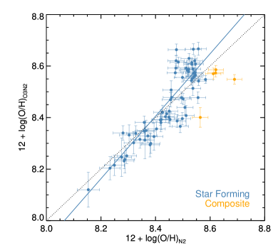
Figure 1: Oxygen abundances estimated with the N2 parameter, compared with those obtained using the O3N2 parameter, for the subsample. Blue and orange dots correspond to star-forming and composite regions, respectively. The dashed line is the identity line, while the solid line is a linear fit to the data.

Values obtained for the 26 objects for which [O iii] $\lambda$5007 is not available are below the low-limit to be defined as AGNs in the [N ii] $\lambda$6583/H$\alpha$ distribution. Hence, we consider these 26 objects as H ii regions too, and we will use their emission lines to estimate their oxygen abundances. Our final sample has a total of 56+4+26=86 H ii regions.

As the faint auroral lines used to compute the electron temperature of the ionized gas (e.g., [O iii] $\lambda$4363) are not detected in any case, we use empirical calibrations (López-Sánchez et al., 2012) to estimate the oxygen abundance. We use $N2$ and $O3N2$ parameters (Alloin et al., 1979), and the calibrations by Marino et al. (2013). With the parameter $O3N2$ we obtain OH${}_{O3N2}=12+\log{(O/H)}_{O3N2}$ for the subsample, and with $N2$, we have OH${}_{N2}=12+\log{(O/H)}_{N2}$ for the full sample. Figure 1 compares OH_O3N2 and OH_N2 for the subsample. A least-squares linear fit yields:

$$OH_{O3N2}=1.15(\pm 0.09)-1.23(\pm 0.77)\times OH_{N2},$$ (4)

(correlation coefficient $r$=0.88), expression used to convert OH_N2 abundances to OH_O3N2 for those 26 regions lacking of $O3N2$ data.

Once OH_O3N2 is determined, we assign an oxygen abundance to the region within each galaxy where its SN Ia was located. For this we use this procedure:

1. In 21 galaxies where several H ii were detected, we estimate a radial oxygen gradient and then we use it to compute the oxygen abundance which corresponds to the projected galactocentric distance at which the SN Ia exploded.

2. For 7 galaxies for which the previous method cannot be applied (i.e., few H ii regions or unreal gradient), we just select the abundance corresponding to the closest region to the SN Ia, being the typical distances $\sim$2-3 kpc.

A typical difference of $\sim 0.05$ dex, smaller that the oxygen abundance error ($~{}0.10$ dex), is found between metallicities derived using gradient or closest region methods, implying their results agree. We finally got the local oxygen abundance for the whole sample of 28 SNe Ia.

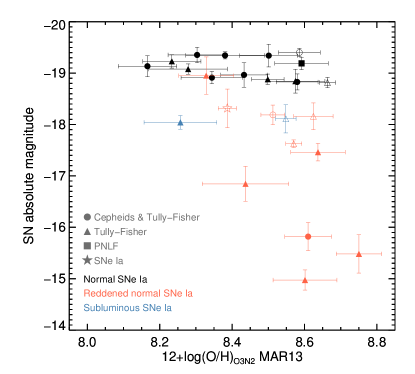
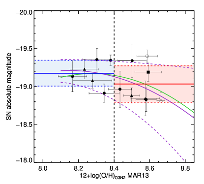
Figure 2: Left: SNe Ia absolute magnitudes, $M_{B}$, as a function of oxygen abundances, $\rm OH_{O3N2}$. Full and open symbols indicate objects with abundances estimated by procedure a) and b), respectively. Triangles, squares and circles indicate the method used to derive distances: Tully-Fisher, PNe Luminosity Function or Tully-Fisher and Cepheids, respectively. The color indicates the type of SN Ia: normal (black), reddened (red), or subluminous (blue). Right: The same plot considering only normal SNe Ia. The green solid line is a second-order polynomial fit to the data. The purple solid line is a second order polynomial fit to four metallicity bins (see text). Short-dashed purple lines represent the 1-$\sigma$ uncertainty to this fit. Blue and red horizontal solid lines provide the averaged value in the low and high metallicity regime, respectively, with their 1-$\sigma$ uncertainty shown with the pale blue and red areas.

3 RESULTS

3.1 Estimation of distances and magnitudes

The distance, $D$, to the galaxies was obtained using the NASA Extragalactic Database, NED, selecting those independent of the SNe Ia method. The apparent magnitudes, $m_{B}$, of SNe Ia in the maximum of their LCs are from Neill et al. (2009), except for SN2014J taken directly as $M_{B}$ from Marion et al. (2015). We have corrected from the Milky Way extinction using the NED values for B-band, $A_{B}$: $m_{B,ext}=m_{B}-A_{B}$. The absolute magnitudes of SNe Ia were computed applying the usual expression: $M_{B}=m_{B,ext}-5\log{D}+5$, ($D$ in pc). No standardization technique has been used to obtain the magnitudes.

3.2 The relation between the SN Ia luminosity and the metallicity

Left panel of Fig. 2 plots SNe Ia absolute magnitudes, $M_{B}$, as a function of the oxygen abundance, $\rm OH_{O3N2}$. This plot indicates SNe Ia located in metal-rich galaxies are less luminous that the ones in metal-poor galaxies. Right panel of Fig. 2 shows the same only considering normal objects (eliminating reddened and sub-luminous SNe Ia as explained in Moreno-Raya et al., 2015), where we have fit a second order polynomial function. We have studied the goodness of this last fit via a $\chi^{2}$ test. As errors in both magnitudes and metallicities are relatively large, we have also considered millions of random variations of the values following a Gaussian distribution of the uncertainties in each axis. In each iteration we fit a second-order polynomial to the data and derive the $\chi^{2}$ of the fit. We sought the minimum values of these values, which confirm the relationship is satisfied with around a 80% of probability.

We have also averaged our data in four metallicity bins: $x<8.2$, $8.2<x<8.4$, $8.4<x<8.6$ and $x>8.6$, being $x=\rm OH_{O3N2}$. The purple continuous line plotted in the right panel of Fig. 2 is a second order polynomial fit to the average value obtained for these bins. This fit matches well with that obtained considering all data. Dividing the abundances into a low-metallicity, $\rm OH_{O3N2}>$8.4, and a high-metallicity, $\rm OH_{O3N2}<$8.4, regime, we find a difference of $0.14\pm 0.10$ mag in $M_{B}$ (blue and red horizontal lines in the right panel of Fig. 2), with high (low) metallicity galaxies hosting less (more) luminous SNe Ia.

A shift in the magnitudes as due to the metallicity effect over the SNe Ia luminosity is theoretically expected. Considering Eqs. 1 to 3, $L\propto f({\rm Z})$, and $M_{bol}=-2.5\log{L}\sim-2.5\log{[f({\rm Z})]}$. Assuming that these equations are also valid in the $B$-band, the difference between the $M_{B}$ of a system with solar abundance and the corresponding $M_{B,{\rm Z}}$ for any other value of Z can be computed using the functions $f({\rm Z})$ given in Eq. 1 and 2. Thus, we get a metallicity-dependent magnitude:

$$M_{B}({\rm Z})=M_{B,{\rm Z}_{\sun}}+\Delta M_{B}({\rm Z})~{}{\rm mag},$$ (5)

where the term $\Delta M_{B}$(Z) produces a shift in the expected value $M_{B}$ which corresponds to Z_⊙.

By using Eqs. 2 and 3, we derive these two metallicity-dependent relationships:

$$\Delta M_{B}({\rm Z})=-2.5\log{\Bigg{(}1-0.075\frac{{\rm Z}}{{\rm Z}_{\odot}}\Bigg{)}}-0.0846\,{\rm mag},$$ (6)

and

$$\Delta M_{B}({\rm Z})=-2.5\log{\Bigg{[}1-0.18\frac{{\rm Z}}{{\rm Z}_{\odot}}\Bigg{(}1-0.10\frac{{\rm Z}}{{\rm Z}_{\odot}}\Bigg{)}\Bigg{]}}$$

$$-0.191\,{\rm mag.}$$ (7)

The terms 0.0846 and 0.191 mag have been introduced to normalize these equations to satisfy $\Delta M_{B}({\rm Z_{\odot}})=0$. Actually, these values represent the magnitude difference between objects with Z=0 and Z=$\rm Z_{\odot}$. As we see, the order of magnitude of these variations, $\sim 0.10-0.20$ mag, agrees with our observational difference of $\sim 0.14\pm 0.10$ mag between the low- and high-metallicity regimes.

3.3 The effect of the color in the $M_{B}$–Z relation

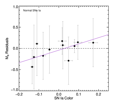
Figure 3: $M_{B}$ residuals after subtracting the fit obtained in Fig.2a as a function of the SNe Ia color. The dashed line marks the zero residuals. The solid purple line is the least squares straight line to the dots.

This probable metallicity dependence of the luminosity of the SN Ia could be attributed to the color correction, a term already included in the cosmological methods to estimate the distance modulus (and implicitly in the determination of the $M_{B}$ of each SN Ia). Actually, the SNe Ia color shows a dependence on the oxygen abundance and there is also a good correlation between SNe Ia magnitudes and their colors (see both in Moreno-Raya et al., 2015). However, when we plot Figure 3 with the $M_{B}$ residuals of the fit found in Fig.2b, as a function of the SNe Ia color, we found, as expected, that there is not a strong correlation, implying that this parameter does not affect very much in the determination of $M_{B}$ for these not reddened objects. A linear fit applied to these points results in:

$$\Delta M_{B}=-0.04\,(\pm 0.12)+1.47\,(\pm 1.42)\times Color$$ (8)

This fit has a correlation coefficient $r$=0.5, and considering the errors of the fit parameters, a no correlation is equally valid or statistically significant. Therefore, in agreement with Childress et al. (2013), the color dependence is not sufficient to explain the correlation seen in Fig. 2, and a metallicity dependence on $M_{B}$ is still left.

We then conclude that a correlation between the absolute magnitude of SNe Ia, $M_{B}$, and their host-galaxy metallicity seems likely. Metal-rich galaxies host less bright SNe Ia than the metal-poor galaxies. This dependence is not included in the term of color when deriving the distance modulus using SNe Ia data.

3.4 Implications of the $M_{B}$–Z relation

If the $M_{B}$-Z relation does actually exist, its most important consequence is that the distances of objects obtained by SNe Ia technique could have a systematic error, as the SNe Ia absolute magnitude has not been accurately estimated.

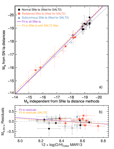
Figure 4: a) $M_{B}$ obtained with distances given by the own SN Ia technique vs $M_{B}$ computed with distances estimated with other independent methods. The dotted line is the $x=y$ line, while purple solid and dashed orange lines are linear fits to the data. b) $M_{B}$ residuals from upper panel vs. metallicity.

Figure 4a shows both magnitudes $M_{B}$ for our SNe Ia sample, as obtained from SN Ia technique distances (taken from NED, prioritizing SALT2 fitter, Guy et al., 2007), and those derived using SNe Ia independent methods, e.g., Cepheids or Tully-Fisher. A linear fit to SALT2 data yields:

$$M_{B,\,{\rm SN\,Ia}}=0.46(\pm 1.59)+1.04(\pm 0.11)M_{B,\,{\rm SN\,Ia~{}ind.}},$$ (9)

(correlation coefficient $r$=0.91). Attending to this figure, and although the slope is close to the unity, the SN Ia technique provides higher luminosities (i.e. higher distances) than the values derived following other methods. That is, luminosities are lower than those predicted by SNe Ia techniques. Figure 4b shows the $M_{B,SNIa}$ residuals a a function of oxygen abundance. A linear fit to SALT2 data (orange line) yields:

$$\Delta M_{B,\,{\rm SN\,Ia}}=2.57(\pm 1.95)-0.30(\pm 0.23){\rm OH_{O3N2}}$$ (10)

This would have an impact on the HD of cosmological models. Since magnitudes estimated by the color and LC parameters provide higher luminosities at high metallicities than they really are, some residuals with a positive slope will be induced in the HD when comparing the luminosity of the SN Ia and the oxygen abundance (or any other metallicity proxy, as the stellar mass following the mass-metallicity relation). Such behavior has been in fact observed, since D’Andrea et al. (2011); Childress et al. (2013) and Pan et al. (2014) found that, once splitting their SNe Ia sample in sub-solar and over-solar metallicity, those located in high-metallicity hosts are, on average, 0.10-0.12 mag brighter than those found in low-metallicity galaxies. Our results explain this fact with a difference of 0.14 $\pm$ 0.10 mag between objects at high and low metallicity host galaxy. In summary, it seems SNe I stretch-color-corrected luminosities have a dependence on the properties of their host galaxies, in particular on the oxygen abundance, which could artificially increase this luminosity above the real value.

Therefore, we here suggest to formally include the metallicity-dependence in the determination of the distance modulus, $\mu$, as:

$$\mu=m_{B}-M_{B}+\alpha\,x_{1}-\beta\,c+\gamma\,{\rm Z},$$ (11)

with $\alpha$, $\beta$ and $\gamma$ being the coefficients for the dependence on stretch, $x_{1}$, color $c$ and metallicity, $Z$, similarly to Lampeitl et al. (2010, Eq.2) and Sullivan et al. (2011), who consider the stellar mass as an extra parameter. It should minimize the small but quantifiable systematic errors induced by the metallicity-dependence of the SNe Ia maximum luminosity.

4 SUMMARY AND CONCLUSIONS

• We estimate oxygen abundances of a sample of 28 local star-forming galaxies hosting SNe Ia, in the region where each one exploded, and study the relation with the maximum magnitude $M_{B}$. Data indicate with a 80% of chance not to be due to random fluctuation, that most metal-rich galaxies seem to host fainter SNe Ia.

• These observational data agree with theoretical predictions from Bravo et al. (2010).

• The existence of such a $M_{B}$-Z relation would naturally explain the observational result after correcting for the LC parameters, that brightest SNe Ia are usually found in metal-rich or massive galaxies. The standard calibration tends to overestimate the maximum luminosities of SNe Ia located in metal-rich galaxies.

This relation, as obtained here with star-forming galaxies, may indicate the metallicity of the progenitor plays a role in the SN Ia luminosity and hence, in the estimated distances. It could also be that the host galaxy extinction, not considered in this work, correlates with the observed O/H. This variation with O/H would induce systematic errors when using SNe Ia to derive cosmological distances.

References

- Alloin et al. (1979) Alloin D., Collin-Souffrin S., Joly M., Vigroux L., 1979, A&A, 78, 200
- Arnett et al. (1982) Arnett W. D., 1982, ApJ, 253, 785
- Asplund et al. (2009) Asplund M., Grevesse N., Sauval A. J., Scott P., 2009, ARA&A, 47, 481
- Baldwin, Phillips & Terlevich (1981) Baldwin J., Phillips M., & Terlevich R., 1981, PASP, 93, 5
- Betoule et al. (2014) Betoule, M., et al., 2014, A&A, 568, 22
- Bravo et al. (2010) Bravo E., Domínguez I., Badenes C., Piersanti L., & Straniero O., 2010, ApJ, 711, L66
- Childress et al. (2013) Childress M., et al., 2013, ApJ, 770, 108
- D’Andrea et al. (2011) D’Andrea, C. B., Gupta, R. R., Sako, M., et al. 2011, ApJ, 743, 172
- Galbany et al. (2014) Galbany, L., 2014, A&A, 572, 38
- Gallagher et al. (2008) Gallagher J. S., Garnavich P. M., Caldwell N., Kirshner R. P., Jha S. W., Li W., Ganeshalingam M., Filippenko A. V., 2008, ApJ, 685, 752
- Gallagher et al. (2005) Gallagher J. S., Garnavich P. M., Berlind P., Challis P., Jha S., Kirshner R. P., 2005, ApJ, 634, 210
- Guy et al. (2007) Guy J., et al., 2007, A&A, 466, 11
- Hamuy et al. (1996a) Hamuy M., Phillips M. M., Suntzeff N. B., Schommer R. A., Maza J., Aviles R., 1996, AJ, 112, 2391
- Hamuy et al. (1996b) Hamuy M., Phillips M. M., Suntzeff N. B., Schommer R. A., Maza J., Smith R. C., Lira P., Aviles R., 1996, AJ, 112, 2438
- Howell et al. (2009) Howell D. A., Sullivan M., Brown E. F., Conley A., Le Borgne D., Hsiao E. Y., Astier P., Balam D., et al. 2009, ApJ, 691, 661
- Iben & Tutukov (1984) Iben Jr., I. & Tutukov A. V., 1984,ApJS, 54, 335
- Kauffmann et al. (2003) Kauffmann G., et al., 2003, MNRAS, 346, 1055
- Kelly et al. (2010) Kelly P. L., Hicken M., Burke D. L., Mandel K. S., & Kirshner R. P. , 2010, ApJ, 715, 743
- Kewley et al. (2001) Kewley L. J., Dopita M. A., Sutherland R. S., Heisler C. A., Trevena J., 2001, ApJ, 556, 121
- Lampeitl et al. (2010) Lampeitl H., Smith M., Nichol R. C., Bassett B., Cinabro D., Dilday B., Foley R. J., Frieman J. A., et al., 2010, ApJ, 722, 566
- Lara-López et al. (2009) Lara-López M. A., Cepa J., Bongiovanni A., Pérez García A. M., Castañeda H., Fernández Lorenzo M., Pović M. & Sánchez-Portal M., 2009, A&A, 505, 529L
- López-Sánchez et al. (2012) López-Sánchez Á. R., Dopita M.A., Kewley L. J., Zahid H. J., Nicholls D. C., and Scharwächter J., 2012, MNRAS, 426, 2630
- Marino et al. (2013) Marino R. A., et al., 2013, A&A, 559, 114
- Marion et al. (2015) Marion, G. H., Sand, D. J., Hsiao, E. Y., et al. 2015, ApJ, 798, 39
- Moreno-Raya et al. (2015) Moreno-Raya M. E., Mollá M., López-Sánchez Á.-R, Galbany L., Vílchez J.M., Domínguez I. & Carnero A., 2015, MNRAS, in prep.
- Neill et al. (2009) Neill J. D., Sullivan M., Howell D. A., Conley A., Seibert M., Martin D. C., Barlow T. A., Foster K., et al. 2009, ApJ, 707, 1449
- Pan et al. (2014) Pan Y.-C., et al., 2014, MNRAS, 438, 1391
- Perlmutter et al. (1999) Perlmutter S., Aldering G., Goldhaber G., Knop R. A., Nugent P., Castro P. G., Deustua S., Fabbro S., et al. & The Supernova Cosmology Project, 1999, ApJ, 517, 565
- Phillips (1993) Phillips M. M., 1993, ApJ, 413, L105
- Phillips et al. (1999) Phillips M. M., Lira P., Suntzeff N. B., Schommer R. A., Hamuy M., & Maza J. 1999, AJ, 118, 1766
- Podsiadlowski et al. (2006) Podsiadlowski P., Mazzali P. A., Lesaffre P., Wolf C., & Forster F., 2006, arXiv:astro-ph/0608324
- Rigault et al. (2013) Rigault, M., 2013, A&A, 560, 66
- Riess et al. (1998) Riess A. G., Filippenko A. V., Challis P., Clocchiatti A., Diercks A., Garnavich P. M., Gilliland R. L., Hogan C. J., et al. ,1998, AJ, 116, 1009
- Hoeflich & Khokhlov (1996) Hoeflich P., Khokhlov A., 1996, ApJ, 457, 500
- Sullivan et al. (2010) Sullivan M., Conley A., Howell D. A., Neill J. D., Astier P., Balland C., Basa S., Carlberg R. G., et al., 2010, MNRAS, 406, 782
- Sullivan et al. (2011) Sullivan M., et al., 2011, ApJ, 737, 102
- Timmes, Brown, & Truran (2003) Timmes F. X., Brown E. F., & Truran J. W., 2003, ApJ, 590, L83
- Travaglio, Hillebrandt, & Reinecke (2005) Travaglio C., Hillebrandt W., Reinecke M., 2005, A&A, 443, 1007
- Webbink (1984) Webbink R. F., 1984, ApJ, 277, 355
- Whelan & Iben (1973) Whelan J. & Iben Jr. I., 1973, ApJ, 186, 1007