Understanding the Alternate Bearing Phenomenon: Resource Budget Model

Abstract

We consider here the resource budget model of plant energy resources, which characterizes the ecological alternate bearing phenomenon in fruit crops, in which high and low yields occur in alternate years. The resource budget model is a tent-type map, which we study in detail. An infinite number of chaotic bands are observed in this map, which are separated by periodic unstable fixed points. These $m$ bands chaotic attractors become $m/2$ bands when the period-$m$ unstable fixed points simultaneously collide with the chaotic bands. The distance between two sets of coexisting chaotic bands that are separated by a period-$1$ unstable fixed point is discussed. We explore the effects of varying a range of parameters of the model. The presented results explain the characteristic behavior of the alternate bearing estimated from the real field data. Effect of noise are also explored. The significance of these results to ecological perspectives of the alternate bearing phenomenon are highlighted.

Major plants which produce large seed crops usually show alternate bearing, i.e., a heavy yield year is followed by extremely light ones, and vice versa. This causes the cascading effect throughout the ecosystem, and may cause the serious health problem for human beings. Therefore, it is very important to understand this natural phenomenon. In this paper we attempt to understand some of the dynamical complexities of this phenomenon. We consider here a simplest mathematical model which captures many of its characteristic behaviors.

I Introduction

Many crop plants of major significance that produce seeded fruit display alternate bearing, in which a year of heavy crop yield, known as a mast year, is followed by a year of extremely light yield and vice versa. This causes a cascading effect throughout the ecosystem, including leading to serious health problems for human beings koenig1 ; koenig2 ; kelly ; monse . The alternate bearing phenomenon is quite common, and has been observed in wild plants in forests as well as domesticated plants. Understanding the dynamics of this natural phenomenon is a difficult task due to the complexities involved in the natural systems, and the limitations of experimental design and verification. In this paper, we attempt to illuminate some of the dynamical complexities of this phenomenon.

Various attempts have been made to determine the characteristics of the alternate bearing phenomenon, including, but not limited to, discussions in Refs. koenig1 ; koenig2 ; kelly ; monse ; isagi ; ken ; satake1 ; satake2 ; satake3 ; ken2 ; rees ; crone ; lyles . However Isagi $et~{}al.$ isagi were the first to attempt to study the characteristics of the phenomenon using a simple mathematical model which captures some of its key behaviors. However, even after this proposition, except for a few attempts isagi ; ken ; satake1 ; satake2 ; satake3 ; ken2 ; rees ; crone ; lyles , this system has not been studied in detail. In this work, we endeavor to study this system in detail and correlate the mathematical model with the ecological behavior. Isagi $et~{}al.$ isagi proposed the following model based on the energy resource present in a plant: a constant amount of photosynthate is produced every year in individual plant. This photosynthate is used for growth and maintenance of the plant. The remaining photosynthate ($P_{s}$) is stored within the plant body. The accumulated photosynthate stored in the plant is expressed as $I$. For a particular year, if the accumulated photosynthate ($I+P_{s}$) exceed a certain threshold $L_{T}$, then the remaining amount $I+P_{s}-L_{T}$ is used for flowering, with the cost of flowering expressed as $C_{f}$ i.e. $C_{f}=I+P_{s}-L_{T}$. These flowers are pollinated and bear fruits, the cost of which is designated as $C_{a}$. Usually, under relatively stable conditions, the fruiting cost is proportional to the cost of flowering, i.e., $C_{a}=RC_{f}$ where $R$ is a proportionality constant. After flowering, the leftover accumulated photosynthate is $L_{T}$. Once fruiting is over, this is reduced to $I^{\prime}=L_{T}-C_{a}$, i.e., $I^{\prime}=-RI+L_{T}(1+R)-P_{s}R$. However, in non-mast years the accumulated energy becomes $I^{\prime}=I+P_{s}$. This phenomenon, considering $I=I_{n}$ and $I^{\prime}=I_{n+1}$, is modeled isagi as follows:

$$I_{n+1} = -RI_{n}+\bar{L}\mbox{~{}~{}~{}~{}~{}}I_{n}>L_{T}-P_{s}$$ (1)

$$= I_{n}+P_{s}\mbox{~{}~{}~{}~{}~{}~{}~{}~{}~{}}I_{n}\leq L_{T}-P_{s}$$

where $n=1,2,3....$ represent the years and $\bar{L}=L_{T}(1+R)-P_{s}R$. Here $R$ is considered as a parameter for this model. Since this model is based on energy (photosynthate) stored in a plant it is termed a resource budget model isagi . Here, we explore the characteristic behavior of this model, considering it significance with reference to previous discussions isagi ; ken ; satake1 ; satake2 ; satake3 ; ken2 ; rees ; crone ; lyles . In this work we explain the reason of existence of chaotic bands and their merging. We found that the $m$ bands chaotic attractors become $m/2$ bands when the period-$m$ unstable fixed points simultaneously collide with the chaotic bands.

In this model $L_{T}$ and $P_{s}$ are generally considered to be constants for mature trees. However, the branches of a natural tree may sometimes be cut, or suffer some destruction, which implies that there must be some variation in $L_{T}$. In addition, due to weather fluctuations or other sources of external disturbances, the yearly photosynthate production, and therefore the quantity $P_{s}$, also does not remain constant. Here, we examine the importance of variations in $L_{T}$ and $P_{s}$ to explore their effects on the characteristic behavior of the system, and correlation with the real-world phenomenon of alternate bearing. Results show that the ratio of cost of fruiting to the cost of flowering, which occurs in multi-bands regime, does not get changed due to the yearly variations in photosynthesis (when yearly photosynthesis exceeds certain critical value). However the initial distance between the chaotic bands does depend on photosynthesis.

This model looks like as a tent map, as shown schematically in Fig. 1(a) ken . However, it can be seen that if $I_{n}$ is below $L_{T}-P_{s}$ then it does not depend on parameter $R$ i.e., the slope is always one. As discussed below, this independence leads to new results compared to standard tent maps tabor ; shameri ; futter – this leads to the creation of separate chaotic bands which are useful for understanding the phenomenon of alternate bearing. Note that this is the simplified model representing the phenomenon of alternate bearing. Shown in Fig. 1(b) is the time-series generated from this model at $R=1.2$ which clearly indicates the high and low fruiting alternatively. Shown in Fig. 1(c) is the number of fruits of an individual Citrus Unshiu tree at the Nebukawa Experimental station in Kanagawa Prefecture over many years. This is an example of alternate bearing at individual level whose high and low fruiting is clearly captured by the model (Fig. 1(b)).

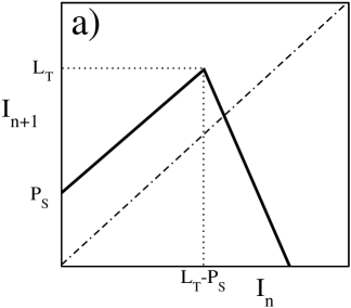
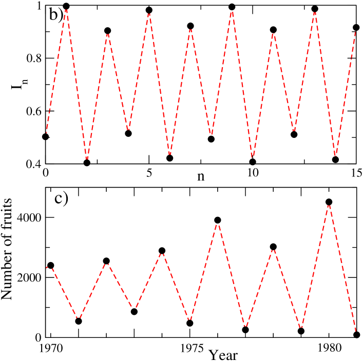
Figure 1: (a) Schematic diagram of the map of the resource budget model of Eq. (1), showing the relationship between the stored photosynthate $I_{n}$ in consecutive years isagi ; ken . Time-series of (b) model Eq. (1) at $R=1.2$ and (c) number of fruits per year of Citrus Unshiu – see text for details.

II Results and discussion

II.1 Generation of Chaos

Fig. 2(a) shows the bifurcation of $I_{n}$ as a function of $R$ in the model, Eq. (1). At low values of $R$ there is only a single stable solution (shown by the red solid line), giving the fixed point of period-1, $I_{*}^{11}$. We will denote the fixed points by $I_{*}^{mj}$, where $j=1,2,...,m$ represents the sequential order of the fixed points of period-$m$. As $R$ increases above 1, the fixed point $I_{*}^{11}$ becomes unstable (shown by the red dashed line). Simultaneously, chaos appears both above and below the period-1 unstable fixed point. The presence of chaos (irregular behavior in $I_{n}$) in these trajectories is confirmed by determining the Lyapunov exponent $\Lambda$ tabor , which is positive for $R>1$ (Fig. 2(b)). Here, upper and lower chaotic bands correspond to the high and low yield years respectively.

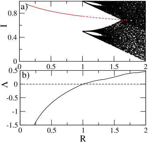
Figure 2: a) The bifurcation diagram, $I_{n}$, and b) the Lyapunov exponent, $\Lambda$ tabor , as a function of parameter $R$ for fixed values of $L_{T}=1$ and $P_{s}=0.5$ in Eq. (1). The dashed line in (a) represents the unstable fixed point of period-1 while in (b) it indicates $\Lambda=0$.

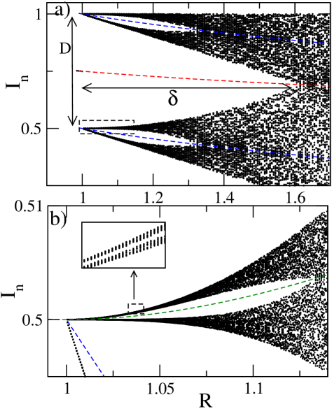
Figure 3: a) The bifurcation diagram of Fig. 2(a) enlarged in the range $R\in[1,1.7]$. b) The expanded view of the dashed box in (a). Inset of (b) corresponds to the small region marked by the dashed box.

We will now try to understand the bifurcation, from stable period-$1$ to chaos, in the model in detail. An expanded view of bifurcation diagram of Fig. 2(a) is shown in Fig. 3(a), over the range $R\in[1,1.7]$. The red dashed line shows the period-$1$ unstable fixed point of the map, Eq. (1). This fixed point is described by

$$I_{*}^{11} = \frac{\bar{L}}{1+R}>L_{T}-P_{s}.$$ (2)

The linear stability analysis of Eq. (1) around this fixed point shows that the eigenvalue $\lambda$ of the stability matrix $M=dI_{n+1}/dI_{n}$ is $\lambda=R$, since $I_{*}^{11}>L_{T}-P_{s}$. Therefore, the fixed point is stable while $R<1$, and unstable for $R>1$. This stable and unstable fixed point is shown as solid and dashed red lines respectively in Figs. 2(a) and 3(b).

At $R=1$, two new fixed points of period-2 emerge. These fixed points given by

$$I_{*}^{21} = \frac{\bar{L}+P_{s}}{1+R}>L_{T}-P_{s}$$

$$I_{*}^{22} = \frac{\bar{L}-P_{s}R}{1+R}\leq L_{T}-P_{s}.$$ (3)

Linear stability analysis at these periodic fixed points indicates that the eigenvalue is $\lambda=R^{2}$. As such, these period-2 fixed points are also unstable for $R\geq 1$. The variation of these fixed points with $R$ is shown as dashed blue lines in Fig. 3(a). These period-2 fixed points pass through two “islands” type of empty space in $I(R$). These islands start near to the respective fixed points of period-2. Note that there are chaotic bands in between the unstable fixed points of period-1 and period-2.

Fig. 3(b) shows an enlargement of the dashed boxed region in Fig. 3(b). Here, another, smaller set of empty islands can be seen. The dashed green line shows the trajectory of one of the unstable fixed points of period-4 which pass though these smaller islands. The period-4 fixed points are given by

$$I_{*}^{41} = \frac{\bar{L}+\bar{L}R^{2}-\bar{L}R+P_{s}}{1+R^{3}}>L_{T}-P_{s}$$

$$I_{*}^{42} = \frac{\bar{L}+\bar{L}R^{2}-\bar{L}R-P_{s}R}{1+R^{3}}>L_{T}-P_{s}$$

$$I_{*}^{43} = \frac{\bar{L}-\bar{L}R+\bar{L}R^{2}+P_{s}R^{2}}{1+R^{3}}>L_{T}-P_{s}$$

$$I_{*}^{44} = \frac{\bar{L}-\bar{L}R+\bar{L}R^{2}-P_{s}R^{3}}{1+R^{3}}\leq L_{T}-P_{s}.$$ (4)

Further expansion of the small region marked by a dashed box in Fig. 3(b) shows another island, as shown in the inset. A period$-8$ fixed point passes across this island.

In general, there are an infinite number of islands, which contain period-$2m$ fixed points, created near to $R=1$. The eigenvalues of these period-$2m$ fixed points are $\lambda\in[R,R^{2m}]$, which are always positive. The exact values depend on the relative values of the fixed points with respect to $L_{T}-P_{s}$, as indicated in Eq. (4). Hence, these fixed points are unstable. This suggests that an infinite number of chaotic bands are created just after $R=1$, separated by one unstable fixed point of period$-2m$ and period$-2(m+1)$. These bands appear in very small regions which are difficult to detect. Shown in Fig. 4 are the zoomed regions of these bands at $R=1.005$ where we can detect up to period-$64$ fixed points, i.e., $128$-chaotic bands.

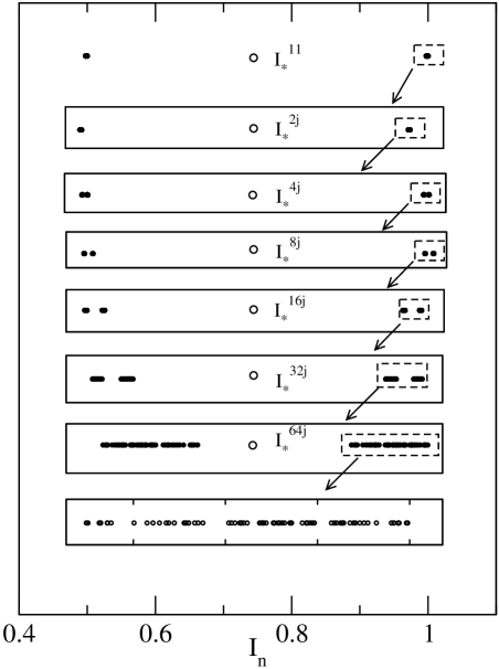
Figure 4: Positions of phase points, $I_{n}$ (filled circles) at $R=1.005$, showing bands of chaos. Arrows indicate the expanded view of smaller regions (dashed boxes). The positions of one of each of the unstable fixed points, $I_{*}^{2mj}$, of period-$2m$ are shown schematically with open circles.

II.2 Separation, $D$, of Chaotic Bands

To understand the complete dynamics of the system of Eq. (1) it is necessary to determine the effect of variation of $P_{s}$. All the infinite bands of chaotic attractors are created just after $R=1$. The bands are separated by period-$2m$ unstable fixed points. The two unstable period-2 fixed points lie above and below the unstable period-1 fixed point, separated near to $R=1$ by a distance $D$, as shown in Fig. 3(a).

$D$ depends only on the distance between the two unstable fixed points of period$-2$. Expanding $\bar{L}$ in terms of $R$, expressions for the two period-$2$ fixed points, Eq. (3), become

$$I_{*}^{21} = L_{T}>L_{T}-P_{s}$$ (5)

$$I_{*}^{22} = L_{T}-P_{s}\leq L_{T}-P_{s}.$$ (6)

This suggests that upper fixed point, $I_{*}^{21}=L_{T}$, is independent of $P_{s}$, while the lower one, $I_{*}^{22}=L_{T}-P_{s}$, varies linearly with $P_{s}$. Therefore, the distance between these two fixed points is $D=|I_{*}^{21}-I_{*}^{22}|=|P_{s}|$, i.e., the starting separation of the chaotic bands which appear above and below the unstable fixed is dependent on $P_{s}$ only. Therefore, similar bifurcation diagrams, as those given in Figs. 2 and 3, are observed for different values $P_{s}$ (figures are shown here). Note that the upper fixed point, $I_{*}^{21}=L_{T}$ is independent of $P_{s}$; hence, irrespective of the values of $P_{s}$, the fixed point remains at $L_{T}$. However, the fixed point $I_{*}^{22}=L_{T}-P_{s}$, which depends on $P_{s}$, moves up to $L_{T}$ as $P_{s}$ decreases.

Ecologically, this dependency of $D$ on $P_{s}$ suggests that, if there is high value of photosynthate in a particular year (for example, with more sunshine, or less snow fall or clouds) then there will be a huge difference in seed output in the following years. This means that, as per the above discussion, the distance $D$, and hence the separation of the upper and lower chaotic bands will be large. This simple model thus explains the important ecological phenomenon of alternate bearing, explaining origin and variation in magnitude of the effect of the alternate bearing. This also predicts that if there is a very high value of yearly photosynthesis, then one can expect alternate bearing to be observed in the next year. Note that if yearly photosynthesis is less in a plant then there will be small fluctuation in $I$ around $L_{T}$, and hence the the magnitude of variations in yields across the years will also be less.

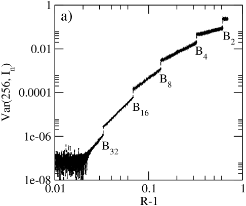
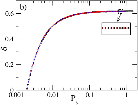
Figure 5: a) Variance in $I_{n}$ after $256$ iterations as a function of $R$. Positions of $B_{2m}$ indicate the $2m-$bands merging crisis. b) Width of $\delta$ regime as a function of $P_{s}$. The black circles and red squares, correspond to the $L_{T}=1$ and $L_{T}=1.5$ respectively. The dashed line is fit to the data by the function Eq. (7).

II.3 Regime of Multi-Band Chaotic Attractors, $\delta$

A closer look at Fig. 3(a) near to $R\sim 1.6$ shows that two bands chaos are merged into a single band when the period-$1$ unstable fixed point collides with the two bands of chaotic attractors. This collision is termed a band-merging crisis grebogi . One method to detect such a crisis is to determine the variance in $I_{n}$ after $2m$-iterations, e. g. within the regime of two bands, the trajectory visits each band alternately, while in the single merged band the trajectory may move anywhere. Therefore, when a crisis occurs there is large jump in the variance of $I_{n}$. This is shown in Fig. 5(a), where a clear jump can be seen at $R\sim 1.6$, when two bands merge. Similarly, at $R\sim 1.3$, four bands of chaotic attractors become two bands, as the upper and lower period-2 unstable fixed points each collide with the attractor bands. Also, sixteen chaotic bands become 8 bands at the point at which the period-8 unstable fixed points collide separately at lower values of $R$. These band merging crises are shown in Fig. 5(a). This figure is generated by finding the variance in $I_{n}$ after $256$ iterations (for detection of crises up to the merging of $128$ bands). Note that, due to the infinitely small width of these bands (as shown in Fig. 4), the higher order merging crisis that it is possible to detect numerically is the merging of the 32 bands containing the period-32 fixed points. This shows that, near to $R=1$, the $m$ bands chaotic attractors become $m/2$ bands when the period-$m$ fixed points simultaneously collide with the chaotic bands. The infinite number of chaotic bands created near to $R=1$ start to merge on further increase of $R$. This process of merging ends when the period-1 fixed point collides with the remaining two bands of chaos near to $R\sim 1.6$. This regime, in which collision occurs, is labeled as $\delta$ in Fig. 3(a), i.e.  from $R=1$ to the values of $R\sim 1.6$ where the two bands of chaos become one band of chaos. In order to see how the width of the multi-band regime $\delta$ changes with $P_{s}$, $\delta$ is numerically determined for different values of $P_{s}$, as shown in Fig. 5(b). The black circles and red squares correspond to the two values of $L_{T}=1$ and $L_{T}=1.5$ respectively. In the inset to Fig. 5(b), it can be seen that the perfect overlapping of these values shows that the variation of $\delta$ with $P_{s}$ is independent of $L_{T}$. A fit to the these curves shows that it is a nonlinear function of the form

$$\delta = a(R-b)\exp({cR^{d}})+e,$$ (7)

where $a,b,c,d,$ and $e$ are fitting parameters. This function is shown for $L_{T}=1$ in Fig. 5(b) as a dashed blue line, with fitting parameters $a=8630.07,b=8632.49,c=-25.945,d=0.0532924,$ and $e=0.615928$ .

One important observation is that at smaller values of $P_{s}$ $(<0.1)$ there is drastic change in $\delta$. However, for large values it becomes saturated around $\delta=0.61$, i.e., $R=1+\delta=1.61$. Note that the alternate bearing occurs when the values of $R$, i.e., ratio of cost of fruiting to the cost of flowering, is in these multi-bands regime (for $\delta>0$). Since $\delta$ is independent of $P_{s}$ (after the photosynthate, $P_{s}>0.1$ which is always expected) implies that $R$ does not get changed due to the yearly variation in photosynthate. One remarkable observation is that this value $R=1+\delta$ is very close to the value of $R=1.34$ estimated from field data rees . Therefore the present analysis explains/supports this important characteristic of ecological alternate bearing phenomenon. The slight deviation in these numerical and experimental values could be due to the external fluctuation as discussed below. Note that this saturation values of $R$ may be different for different type of plants, and may depends on regions and climates rees – which needs to be probed further.

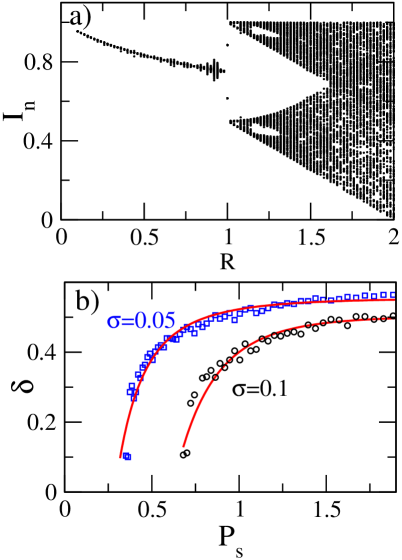
Figure 6: a) The bifurcation diagram as a function of parameter $R$, with noise level $\sigma=0.05$ (5%). b) Width of $\delta$ regime as a function of $P_{s}$ at noise levels $\sigma=0.05$ (5%) (blue squares) and $\sigma=0.1$ (10%) (black circles). Fittings to the data using function Eq. (7) are shown by solid red lines.

II.4 Effects of Noise

Natural systems are rarely free from external perturbations. Therefore, in order to fully understand the dynamics of this system, we must also consider the effect of noise. Here, we consider uniformly distributed random noise in $I_{n}$, with values between $[0,1]$ and strength $\sigma$. We add this noise after each iteration of the map, Eq. (1), i.e., $I_{n}=I_{n}+\sigma\times[0,1]$. Fig. 6(a) shows the bifurcation diagram generated with noise of strength $\sigma=0.05$ ($5\%$ of signal $I$) for fixed $L_{T}=1$ and $P_{s}=0.5$. The features remain similar to those without noise, Fig. 2(a). The islands and the distance $D$ still persist under noise.

To understand the effects of the variations of $P_{s}$ cause by this noise, two data sets are shown in Fig. 6(b), with black-circles and blue-squares representing data for noise levels $\sigma=0.1$ (10%) and $\sigma=0.05$ (5%) respectively. The fits to these datasets, using the function Eq. (7), show similar trends to that without noise (Fig. 5). However, the saturation distance $\delta$ decreases for higher strength of noise. Therefore, the results presented in this work reveals that, under natural conditions in which fluctuations always exist, the characteristic properties $D$ and $\delta$ of alternate bearing phenomenon can persist.

III Conclusions

Piecewise-smooth dynamical systems, which model many natural phenomena, are well studied and found to be important to understand the systems. Piecewise-linear maps have been also well studied (see recent paper futter and references therein). Here, we have studied the resource budget model which captures the phenomenon of alternate bearing in plants. However the map we considered here, Eq. (1), is different to standard tent maps futter ; shameri . In this model, one side ($I_{n}\leq L_{T}-P_{s}$) has a constant coefficient linear equation, while in all reported works the slopes of both sides change. Therefore this work adds a new class of map to tent-type maps, and we were able to study the variations of $D$ and $\delta$. From a mathematical point of view, it is important to study this new class of tent map in detail. This system shows rich bifurcation behavior, where infinite islands containing period-$2m$ unstable orbits are observed. The islands are destroyed due to band merging crises when the unstable fixed points collide with chaotic bands.

We found that the distance $D$ only depends on $P_{s}$ and independent of $L_{T}$. This suggests that if there is a high value of photosynthate in a year then there will be a huge difference in seed output in the next year. This variation is independent of the threshold value $L_{T}$ of the individual tree. Therefore, this simple model demonstrates the characteristic properties of an ecological phenomenon, explaining the magnitude and variation of alternate bearing.

We observe that only for smaller values of $P_{s}$ there is drastic change in $\delta$. However, for large values $\delta$ is saturated at approximately $R=1.61$, which is very close to estimations from real data rees . This shows that variations in the ratio of cost of fruiting to cost of flowering does not dependent on the amount of photosynthate.

These results, the independence of $L_{T}$ on $D$ and the saturation of regime of multi-bands, may be useful for ecological perspectives and hence its open up to new challenges for further analysis and verification in experimental situations. These analysis may also be extended to other types of important systems satake1 . It will be also interesting to explore these analysis in coupled systems where masting (synchronized production) occurs isagi ; satake1 ; satake2 ; rees ; satoh .

Acknowledgment: AP acknowledges support from JSPS Invitation Fellowship, Japan and thanks the TUAT, Fuchu Campus, Tokyo for warm hospitality.

References

- (1) W. D. Koenig and J. M. H. Knopes, American Scientist, 93, 340 (2005).
- (2) W. D. Koenig, M. H. Knopes, W. J. Carmen and I. S. Pearse, Ecology, 96, 184 (2015).
- (3) D. Kelly and V. L. Sork, Annu. Rev. Ecol. Syst. 33, 427 (1002).
- (4) S. P. Monselise and E. E. Goldschmidt, Horticulture Review, 4, 128 (2011).
- (5) Y. Isagi, K. Sugimura, A. Sumida and H. Ito, J. Theor. Biol. 187, 231 (1997).
- (6) X. Ye and K. Sakai, Chaos, 23, 043124 (2013).
- (7) D. Lyles, T. S. Rosenstock, A. Hasting and P. H. Brown, J. Theor. Biol. 259, 701 (2009).
- (8) E. E. Crone, L. Polansky, and P. Lesica, The American Naturalist, 166, 396 (2005).
- (9) M. Rees, D. Kelly, and O. N. Bjornstad, The American Naturalist, 160, 44 (2002).
- (10) K. Sakai, Nonlinear Dynamics and Chaos in Agriculture Systems, (Elsevier Science, Amsterdam, 2001).
- (11) A. Satake and Y. Iwasa, J. Theor. Biol. 203, 63 (2000).
- (12) A. Satake and Y. Iwasa, Ecology 83, 993 (2002).
- (13) A. Satake and Y. Iwasa, J. Ecology 90, 830 (2002).
- (14) W. F. H. Al-shameri and M. A. Mahiub, I. J. Math. Analysis, 7 1433 (2013).
- (15) B. Futter, V. Avrutin and M. Schanz, Chaos, Solitons & Fractals, 45, 465 (2012).
- (16) M. Tabor, Chaos and Integrability in Nonlinear Dynamics: An Introduction, (Wiley-Blackwell, 1989).
- (17) C. Grebogi, E. Ott, F. Romeiras and J. A. Yorke, Phys. Rev. A 35, 5365 (1987).
- (18) K. Satoh and T. Aihara, J. Phys. Soc. Japan, 59, 1184 (1990).