The Lyman alpha reference sample.
VII. Spatially resolved H$\alpha$ kinematics

We present integral field spectroscopic observations with the Potsdam Multi Aperture Spectrophotometer of all 14 galaxies in the $z\sim 0.1$ Lyman Alpha Reference Sample (LARS). We produce 2D line of sight velocity maps and velocity dispersion maps from the Balmer $\alpha$ (H$\alpha$) emission in our data cubes. These maps trace the spectral and spatial properties of the LARS galaxies’ intrinsic Ly$\alpha$ radiation field. We show our kinematic maps spatially registered onto the Hubble Space Telescope H$\alpha$ and Lyman $\alpha$ (Ly$\alpha$) images. Only for individual galaxies a causal connection between spatially resolved H$\alpha$ kinematics and Ly$\alpha$ photometry can be conjectured. However, no general trend can be established for the whole sample. Furthermore, we compute non-parametric global kinematical statistics – intrinsic velocity dispersion $\sigma_{0}$, shearing velocity $v_{\mathrm{shear}}$, and the $v_{\mathrm{shear}}/\sigma_{0}$ ratio – from our kinematic maps. In general LARS galaxies are characterised by high intrinsic velocity dispersions (54 km s^-1 median) and low shearing velocities (65 km s^-1 median). $v_{\mathrm{shear}}/\sigma_{0}$ values range from 0.5 to 3.2 with an average of 1.5. Noteworthy, five galaxies of the sample are dispersion dominated systems with $v_{\mathrm{shear}}/\sigma_{0}<1$ and are thus kinematically similar to turbulent star forming galaxies seen at high redshift. When linking our kinematical statistics to the global LARS Ly$\alpha$ properties, we find that dispersion dominated systems show higher Ly$\alpha$ equivalent widths and higher Ly$\alpha$ escape fractions than systems with $v_{\mathrm{shear}}/\sigma_{0}>1$. Our result indicates that turbulence in actively star-forming systems is causally connected to interstellar medium conditions that favour an escape of Ly$\alpha$ radiation.

1 Introduction

As already envisioned by Partridge & Peebles (1967) the hydrogen Lyman $\alpha$ (Ly$\alpha$, $\lambda_{\mathrm{Ly\alpha}}=1215.67$Å) line has become a prominent target in succsesful systematic searches for galaxies in the early Universe. Redshifted into the optical, this narrow high equivalent width line provides enough contrast to be effectively singled out in specifically designed observational campaigns. As of yet mostly narrow-band selection techniques have been employed (e.g. Hu et al. 1998; Taniguchi et al. 2003; Malhotra & Rhoads 2004; Shimasaku et al. 2006; Tapken et al. 2006; Gronwall et al. 2007; Ouchi et al. 2008; Grove et al. 2009; Shioya et al. 2009; Hayes et al. 2010; Ciardullo et al. 2012; Sandberg et al. 2015), but multi-object and integral-field spectroscopic techniques are now also frequently used to deliver large Lyman $\alpha$ emitter (LAE) samples (Cassata et al. 2011; Adams et al. 2011; Mallery et al. 2012; Cassata et al. 2015; Bacon et al. 2015). Moreover, all galaxy redshift record holders in the last decade were spectroscopically confirmed by virtue of their Ly$\alpha$ line (Iye 2011; Ono et al. 2012; Finkelstein et al. 2013; Oesch et al. 2015; Zitrin et al. 2015) and a bright LAE at $z=6.6$ is even believed to contain a significant amount of stars made exclusively from primordial material (so called Pop-III stars, Sobral et al. 2015).

As important as Ly$\alpha$ radiation is in successfully unveiling star formation processes in the early Universe, as notoriously complicated appears its correct interpretation. Resonant scatterings in the interstellar and circum-galactic medium diffuse the intrinsic Ly$\alpha$ radiation field in real and frequency space. These scatterings also increase the path length of Ly$\alpha$ photons within a galaxy and consequently Ly$\alpha$ is more susceptible for being destroyed by dust (see Dijkstra 2014, for a comprehensive review covering the Ly$\alpha$ radiative transfer fundamentals). Consequently, a galaxy’s Ly$\alpha$ observables are influenced by a large number of its physical properties. Understanding these influences is crucial to correctly interpret high-$z$ LAE samples. In other words, we have to answer the question: What differentiates an LAE from other star-forming galaxies that do not show Ly$\alpha$ in emission?

Regarding Ly$\alpha$ radiation transport in individual galaxies, a large body of theoretical work investigated analytically and numerically how within simplified geometries certain parameters (e.g. density, temperature, dust content, kinematics and clumpiness) affect the observed Ly$\alpha$ radiation field (e.g. Neufeld 1990; Ahn et al. 2003; Dijkstra et al. 2006; Verhamme et al. 2006; Laursen et al. 2013; Gronke & Dijkstra 2014; Duval et al. 2014). Commonly a spherical shell model is adopted. In this model a thin shell of expanding, contracting or static neutral gas represents the medium responsible for scattering Ly$\alpha$ photons. As a result from scattering in the shell complex Ly$\alpha$ line morphologies arise and the expansion velocity and the neutral hydrogen column density of the shell are of pivotal importance in shaping the observable Ly$\alpha$ line. By introducing deviations from pure spherical symmetry Zheng & Wallace (2014) and Behrens et al. (2014) show that the observed Ly$\alpha$ properties also depend on the viewing angle under which a system is observed. The latter result is also found in large-scale cosmological simulations that were post-processed with Ly$\alpha$ radiative transport simulations (e.g. Laursen & Sommer-Larsen 2007; Laursen et al. 2009; Barnes et al. 2011). Recently more realistic hydro dynamic simulations of isolated galaxies have been paired with Ly$\alpha$ radiation transport simulations (Verhamme et al. 2012; Behrens & Braun 2014). These studies underline again the viewing angle dependence of the Ly$\alpha$ observables. In particular they show, that disks observed face-on are expected to exhibit higher Ly$\alpha$ equivalent widths and Ly$\alpha$ escape fractions than if they were observed edge on. More importantly, these state of the art simulations also emphasise the importance of small-scale interstellar medium structure that was previously not included in simple models. For example Behrens & Braun (2014) demonstrate how supernova-blown cavities are able to produce favoured escape channels for Ly$\alpha$ photons.

Observationally, when Ly$\alpha$ is seen in emission, the spectral line profiles can be typified by their distinctive shapes. In a large number of LAE spectra the Ly$\alpha$ line often appears asymmetric, with a relatively sharp drop on the blue and a more extended wing on the red side. A significant fraction of spectra also shows characteristic double peaks, with the red peak often being stronger than the blue (e.g. Tapken et al. 2004, 2007; Yamada et al. 2012; Hong et al. 2014; Henry et al. 2015; Yang et al. 2015). Interestingly, a large fraction of double peaked and asymmetric Ly$\alpha$ profiles appear well explained by the spherical symmetric scenarios mentioned above. Double-peaked profiles are successfully reproduced by slowly-expanding shells ($v_{\mathrm{exp}}\lesssim 100$ km s^-1) or low neutral hydrogen column densities $N_{\mathrm{{H\textsc{i}}}}\lesssim 10^{19}$cm^-2, while high expansion velocities ($v_{\mathrm{exp}}\sim 150\,$–$\,300$ km s^-1) with neutral hydrogen column densities of $N_{\mathrm{{H\textsc{i}}}}\gtrsim 10^{20}$cm^-2 produce the characteristic asymmetric profile with an extended red wing (Tapken et al. 2006, 2007; Verhamme et al. 2008; Schaerer et al. 2011; Gronke & Dijkstra 2014).

Further observational constraints on the kinematics of the scattering medium can be obtained by measuring the offset from non-resonant rest-frame optical emission lines (e.g. H$\alpha$ or [O III]) to interstellar low-ionisation state metal absorption lines (e.g. O i $\lambda 1302$ or Si ii $\lambda 1304$). While the emission lines provide the systemic redshift, some of the low-ionisation state metal absorption lines trace the kinematics of cold neutral gas phase. Both observables are challenging to obtain for high-$z$ LAEs and require long integration times on 8–10 m class telescopes (e.g. Shapley et al. 2003; Tapken et al. 2004) or even additional help from gravitational lenses (e.g. Schaerer & Verhamme 2008; Christensen et al. 2012). As the continuum absorption often remains undetected, just the offset between the rest-frame optical lines and the Ly$\alpha$ peaks are measured (e.g. McLinden et al. 2011; Guaita et al. 2013; Erb et al. 2014). Curiously, the observed Ly$\alpha$ profiles also agree well with those predicted by the simple shell model, when the measured offsets (typically $\Delta v\sim 200$ km s^-1) are associated with shell expansion velocities in the simple shell model (Verhamme et al. 2008; Hashimoto et al. 2013; Song et al. 2014; Hashimoto et al. 2015). Only few profiles appear incompatible with the expanding shells (Chonis et al. 2013). These profiles are characterised by extended wings or bumps in the blue side of the profile (Martin et al. 2014; Henry et al. 2015). However, given aforementioned viewing angle dependencies in more complex scenarios, this overall success of the simple shell model appears surprising and is therefore currently under scrutiny (Gronke et al. 2015). Nevertheless, at least qualitatively the observations demonstrate in concert with theoretical predictions that LAEs predominantly have outflow kinematics and that such outflows promote the Ly$\alpha$ escape (see also Kunth et al. 1998; Mas-Hesse et al. 2003).

Kinematic information is moreover encoded in the rest-frame optical line emission alone. These emission lines trace the ionised gas kinematics and especially the hydrogen recombination lines such as H$\alpha$ relate directly to the spatial and spectral properties of a galaxy’s intrinsic Ly$\alpha$ radiation field. Therefore spatially resolved spectroscopy of a galaxy’s H$\alpha$ radiation field constrains the initial conditions for the subsequent Ly$\alpha$ radiative transfer through the interstellar, circum-galactic, and intergalactic medium to the observer. But at high $z$ most LAEs are so compact that they cannot be spatially resolved from the ground and hence in the analysis of the integrated spectra all spatial information is lost. Resolving the intrinsic Ly$\alpha$ radiation of typical high-$z$ LAEs spatially and spectrally at such small scales would require integral field spectroscopy, preferably with adaptive optics, in the near infrared with long integration times. Although large samples of continuum-selected $z\sim 2-3$ star-forming galaxies have already been observed with this method (see Glazebrook 2013, for a comprehensive review), little is known about the Ly$\alpha$ properties of the galaxies in those samples.

In the present manuscript we present first results obtained from our integral-field spectroscopic observations with the aim to relate spatially and spectrally resolved intrinsic Ly$\alpha$ radiation field to its observed Ly$\alpha$ properties. Therefore we targeted the H$\alpha$ line in all galaxies of the $z\sim 0.03$ – $0.18$ Lyman Alpha Reference Sample (hereafter LARS). LARS consists of 14 nearby laboratory galaxies, that have far-UV (FUV, $\lambda\sim$ 1500Å) luminosities similar to those of high-$z$ star-forming galaxies. Moreover, to ensure a strong intrinsic Ly$\alpha$ radiation field, galaxies with large H$\alpha$ equivalent widths were selected ($\mathrm{EW}_{\mathrm{H\alpha}}\geq 100$Å). The backbone of LARS is a substantial program with the Hubble Space Telescope. In this program each galaxy was observed with a combination of ultra-violet long pass filters, optical broad band filters, as well as H$\alpha$ and H$\beta$ narrow-band filters. These images were used to accurately reconstruct Ly$\alpha$ images of those 14 galaxies. Moreover, UV-spectroscopy with HSTs Cosmic Origins Spectrograph (COS) is available for the whole sample.

This paper is the seventh in a series presenting results of the LARS project. In Östlin et al. (2014) (hereafter Paper I) we detailed the sample selection, the observations with HST and the process to reconstruct Ly$\alpha$ images from the HST data. In Hayes et al. (2014) (hereafter Paper II) we presented a detailed analysis of the imaging results. We found that 6 of the 14 galaxies are indeed analogous to high-$z$ LAEs, i.e. they would be selected by the conventional narrow-band survey selection requirement: $\mathrm{EW}_{\mathrm{Ly\alpha}}>20$ Å. The main result of Paper II is that a galaxy’s morphology seen in Ly$\alpha$ is usually very different compared to its morphological appearance in H$\alpha$ and the FUV; especially Ly$\alpha$ is often less centrally concentrated and so these galaxies are embedded in a faint low surface-brightness Ly$\alpha$ halo. The results in Paper II (see also Hayes et al. 2013) therefore provide clear observational evidence for resonant scattering of Ly$\alpha$ photons in the neutral interstellar medium. 21cm observations tracing the neutral hydrogen content of the LARS galaxies were subsequently presented in Pardy et al. (2014) (hereafter Paper III) and the results supported the complex coupling between Ly$\alpha$ radiative transfer and the properties of the neutral medium. In Guaita et al. (2015) (hereafter Paper IV) the morphology of the LARS galaxies was thoroughly re-examined. By artificially redshifting the LARS imaging data-products, we were able to confirm that morphologically LARS galaxies indeed resemble $z\sim 2-3$ star forming galaxies. Rivera-Thorsen et al. (2015) (herafter Paper V) then presented high-resolution far-UV COS spectroscopy of the full sample. Analysing the neutral-interstellar medium kinematics as traced by the low-ionisation state metal absorption lines, we showed that all galaxies with global Ly$\alpha$ escape fractions $>$5% appear to have outflowing winds. Finally in Duval et al. (2015, A&A submitted - hereafter Paper VI) we performed a detailed radiative transfer study of one LARS galaxy (Mrk 1468 - LARS 5) using all the observational constraints assembled within the LARS project, also including the data that is presented in this paper. In particular we show that this galaxy’s spatial and spectral Ly$\alpha$ emission properties are consistent with scattering of Ly$\alpha$ photons by outflowing cool material along the minor axis of the disk.

In the here presented first analysis of our LARS integral-field spectroscopic data we focus on a comparison of results obtainable from spatially resolved H$\alpha$ kinematics to results from the LARS HST Ly$\alpha$ imaging and 21cm H i observations. In a subsequent publication (Orlitova, in prep.) we will combine information from our 3D H$\alpha$ spectroscopy with our COS UV spectra to constrain the parameters of outflowing winds.

We note, that this paper is not the first in relating observed spatially resolved H$\alpha$ observations to a local galaxy’s Ly$\alpha$ radiation field. Recently in a pioneering study exploiting MUSE (Bacon et al. 2014) science-verification data, Bik et al. (2015) showed, that an asymmetric Ly$\alpha$ halo around the main star-forming knot of ESO338-IG04 (Hayes et al. 2005; Östlin et al. 2009; Sandberg et al. 2013) can be linked to outflows seen in the H$\alpha$ radial velocity field. Moreover, the kinematic constraints provided by our observations were already used for modelling the Ly$\alpha$ scattering in one LARS galaxy (Paper VI), and also here galactic scale outflows were required to explain the galaxy’s Ly$\alpha$ radiation. With the full data set presented here, we now study whether such theoretical expected effects are indeed common among Ly$\alpha$-emitting galaxies.

The outline of this manuscript is as follows: In Sect. 2 our PMAS observations of the LARS sample are detailed. The reduction of our PMAS data is explained in Sect. 3. Ancillary LARS data products used in this manuscript are described briefly in Sect. 4. The derivation and analysis of the H$\alpha$ velocity and dispersion maps is presented in Sect. 5. In Sect. 6 the results are discussed and finally we summarise and conclude in Sect. 7. Notes on individual objects are given in Appendix A.

2 PMAS Observations

Table 1: Log of PMAS lens array observations of the LARS sample.

LARS	Observing-	$t_{\mathrm{exp.}}$	FoV	$\lambda$-Range	Resolving Power	Seeing	Observing-
ID	Date	[s]	[arcsec2]	$\lambda_{\mathrm{start}}-\lambda_{\mathrm{end}}$ [Å]	$\overline{R}_{\mathrm{FWHM}}$	FWHM [″]	Conditions
1	2012-03-16	2$\times$1800 s	16$\times$16	5948 - 7773	5306	1.8	phot.
2	2012-03-15	2$\times$1800 s	16$\times$16	5752 - 7581	5205	1.1	non-phot.
3	2012-03-14	3$\times$1800 s	16$\times$16	5948 - 7773	5362	1.1	phot.
4	2012-03-13	3$\times$1800 s	16$\times$16	5752 - 7581	5883	1.0	phot.
5	2012-03-14	3$\times$1800 s	8$\times$8	5874 - 7700	5886	1.3	phot.
6	2012-03-13	2$\times$1800 s	16$\times$16	5752 - 7581	5865	1.0	phot.
7	2012-03-16	3$\times$1800 s	16$\times$16	5948 - 7773	3925	1.3	non-phot.
8	2012-03-15	3$\times$1800 s	16$\times$16	5948 - 7773	4415	0.9	non-phot.
9	2012-03-12	3$\times$1800 s	16$\times$16	5752 - 7581	5561	0.9	phot.
	2012-03-14	3$\times$1800 s	16$\times$16	5948 - 7773	4772	0.9	non-phot.
10	2012-03-14	2$\times$1800 s	8$\times$8	5874 - 7700	5438	1.5	phot.
11	2012-03-15	3$\times$1800 s	16$\times$16	5948 - 7773	4593	1.0	non-phot.
12	2012-03-14	3$\times$1800 s	8$\times$8	6553 - 8363	6756	0.9	phot.
13	2011-10-02	4$\times$1800 s	8$\times$8	6792 - 8507	7766	1.2	phot.
	2011-10-02	4$\times$1800 s	8$\times$8	6792 - 8507	7771	1.2	phot.
14	2012-03-13	2$\times$1800 s	8$\times$8	6553 - 8363	7718	0.9	phot.

We observed all LARS galaxies using the Potsdam Multi-Aperture Spectrophotometer (PMAS; Roth et al. 2005) at the Calar Alto 3.5 m telescope during 4 nights from March 12 to March 15, 2012 (PMAS run212), except for LARS 13, which was observed on October 10 2011 (PMAS run197). PMAS was used in the lens array configuration, where 256 fibers are coupled to a $16\times 16$ lens array that contiguously samples the sky. Depending on the extent of the targeted galaxy we used either the standard magnification mode, that provides an 8″$\times$8″ field of view (FoV) or the double magnification mode, where the FoV is 16″$\times$16″. The backward-blazed R1200 grating was mounted on the spectrograph. To ensure proper sampling of the line spread function the 4k$\times$4k CCD (Roth et al. 2010) was read out unbinned along the dispersion axis. This setup delivers a nominal resolving power from $R\sim 5000$ to $R\sim 8000$ within the targeted wavelength ranges. In Sect. 3.3 we will show that while the nominal resolving powers are met on average, the instrumental broadening varies at small amplitudes from fibre to fibre.

On-target exposures were usually flanked by 400 s exposures of empty sky near the target. These sky frames serve as a reference for removing the telluric background emission. Due to an error in our observing schedule, no sky frames were taken for LARS 4, LARS 7 and LARS 9 (2012-03-12 pointing). Fortunately, this did not render the observations unusable, since there are enough blank-sky spectral pixels (so called spaxels) within those on-target frames to provide us with a reference sky (see paragraph on sky subtraction in Sect. 3).

Observing blocks of one hour were usually flanked by continuum and HgNe arc lamp exposures used for wavelength and photometric calibration. We obtained several bias frames throughout each night when the detector was idle during target acquisition. Spectrophotometric standard stars were observed at the beginning and at the end of each astronomical night (BD+75d325 & Feige 67 from Oke 1990, $t_{\mathrm{exp.}}=600$ s). Twilight flat exposures were taken during dawn and dusk.

In Table 2 we provide a log of our observations. By changing the rotation of the grating, we adjusted the wavelength ranges covered by the detector, such that the galaxies H$\alpha$ - [N ii] complex is located near the center of the CCD. Note, that $\pm 350$Å at the upper/lower end of the quoted spectral ranges are affected by vignetting (a known “feature” of the PMAS detector - see Roth et al. 2010). We also quote the average spectral resolution of our final datasets near H$\alpha$. The determination of this quantity is described in Sect. 3.3. The tabulated seeing values refer always to the average FWHM of the guide star PSF measured during the exposures with the acquisition and guiding camera of PMAS. This value is on average $\approx 0.2$″ higher than the DIMM measurements (see also Husemann et al. 2013).

In Fig. 1 we show the wavelengths of the redshifted H$\alpha$ line for all LARS galaxies overlaid on the typical night sky emission spectrum at Calar Alto from Sánchez et al. (2007a). As can be seen for two galaxies (LARS 13 and LARS 14) the H$\alpha$ line signal is contaminated by telluric line emission and two other galaxies (LARS 9 and LARS 12) have their H$\alpha$ line within an absorption band. This, however, has no effect on the presented analysis. For LARS 13 and LARS 14 we could optimally subtract the interfering sky-lines from the science exposures using the separate sky frames. Moreover, as we use only spaxels with high signal to noise H$\alpha$ lines in our analysis (cf. Sect. 5), the high frequency changes within the telluric absorption bands do not alter the quantified features – width and peak position – of the profiles.

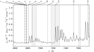
Figure 1: Wavelengths of the redshifted H$\alpha$ lines of the LARS galaxies (vertical dashed lines) compared to the night sky emission spectrum at Calar Alto (Sánchez et al. 2007a). Grey regions indicate the telluric absorption bands (O₂ B-Band: 6887 Å - 6919 Å, O₂ A-Band: 7607 Å - 7633 Å, and H₂O a-Band: 7168 Å - 7304 Å, see e.g. Cox 2000).

3 PMAS data reduction

3.1 Basic reduction with p3d

For reducing the raw data the p3d-package (Sandin et al. 2010, 2012) was utilized. This pipeline covers all basic steps needed for reducing fiber-fed integral field spectroscopic data: bias subtraction, flat fielding, cosmic ray removal, tracing and extraction of the spectra, correction of differential atmospheric refraction and co-addition of exposures (see also Turner 2010). We now describe how we applied the tasks of p3d on our raw data for each of these steps:

• Bias subtraction: Master bias frames were created by p3d_cmbias. These master bias frames were then subtracted from the corresponding science frames. Visual inspection of the bias subtracted frames showed no measurable offsets in unexposed regions between the 4 quadrants of the PMAS CCD, which attests optimal bias removal.

• Flat fielding: Each of the 256 fibers has its own wavelength dependent throughput curve. To determine these the task p3d_cflatf was applied on the twilight flats. The determined curves are then applied in the extraction step of the science frame (see below) to normalize the extracted spectra.

• Cosmic ray removal: Cosmic ray hits on the CCD were removed with p3d_cr. Visual inspections guided by the parameter study of Husemann et al. (2012) lead us to apply the L.A. Cosmic algorithm (van Dokkum 2001) with $\sigma_{\mathrm{lim}}=5$, $\sigma_{\mathrm{frac}}=1$, $f_{\mathrm{lim}}=15$, a grow radius of 2 and a maximum of 4 iterations.

• Tracing and extraction: Spectra were extracted with the modified Horne (1986) optimal extraction algorithm (Sandin et al. 2010). The task p3d_ctrace was used to determine the traces and the cross-dispersion profiles of the spectra on the detector. Spectra were then extracted with p3d_cobjex, also using the median recentering recommended in Sandin et al. (2012).

• Wavelength calibration: With p3d_cdmask we obtained dispersion solutions (i.e. mappings from pixel to wavelength space) from the HgNe lamp frames using a sixth-order polynomial. The wavelength sampling of the extracted science spectra is typically 0.46 Å px^-1. We further improved the wavelength calibration of the science frames by applying small shifts (typically $0.1$ – $0.3$ px) determined from the strong 6300Å and 6364Å [O i] sky lines (not available within the targeted wavelength range for LARS 12, 13, and 14)

• Sensitivity function and flux calibration: Using extracted and wavelength-calibrated standard star spectra, we created a sensitivity function utilizing p3d_sensfunc. Absorption bands in the standard star spectra as well as telluric absorption bands (see Fig. 1) were masked for the fit. Extinction curves were created using the empirical formula presented in Sánchez et al. (2007b) using the extinction in $V$-band as measured by the Calar Alto extinction monitor. We flux-calibrated all extracted and wavelength-calibrated science frames with the derived sensitivity function and extinction curve using p3d_fluxcal.

The final data products from the p3d-pipeline are flux- and wavelength-calibrated data cubes for all science exposures, as well as the corresponding error cubes. From here we now perform the following reduction steps with our custom procedures written in python.

3.2 Sky subtraction and co-addition

• Sky subtraction: All sky frames were reduced like science frames as described in the previous section. These extracted, wavelength- and flux-calibrated sky frames were then subtracted from the corresponding science frames and errors were propagated accordingly. Unfortunately, no separate sky exposures were taken for three targets (LARS 4, LARS 7 and LARS 9, cf. Sect. 2). For these targets we created a narrow band image of the H$\alpha$-[N ii] region by summing up the relevant layers in the datacube. In this image we selected spaxels that do not contain significant amounts of flux. From these spaxels then an average sky spectrum was created, which was then subtracted from all spaxels. As the spectral resolution varies across the FoV (cf. Sect. 3.3), this method produces some residuals at the position of the sky lines, which however do not touch the H$\alpha$ lines of the affected targets.

• Stacking: We co-added all individual flux-calibrated and sky-subtracted data cubes using the variance-weighted mean. For this calculation the input variances were derived from squaring the error cubes. Before co-addition we ensured by visual inspection that there are no spatial offsets between individual exposures.

3.3 Spectral resolving power determination

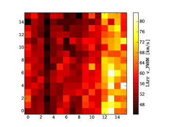
Figure 2: Representative resolving power map for the observation of LARS 1. The resoultion is expressed as $v_{\mathrm{FWHM}}$ of a 1D Gaussian fit. Black spaxels at the positions $(x,y)=(0,14)$ and $(8,15)$ are dead fibres.

To determine the intrinsic width of our observed H$\alpha$ lines we need to correct for instrumental broadening by the spectrograph’s line spread function (the spectrograph’s resolving power, Robertson 2013). It is known that for PMAS the resolving power varies from fibre to fibre and with wavelength (e.g. Sánchez et al. 2012). To determine the broadening at the wavelength of the H$\alpha$ line we use the HgNe arc lamp exposures, which were originally used to wavelength calibrate the on-target exposures. We first create wavelength-calibrated data cubes from these arc frames. Next we select two strong arc lamp lines which are nearest in wavelength to the corresponding galaxy’s H$\alpha$ line. Finally, we fit 1D Gaussians in each spaxel to each of those lines (e.g. similar as in Alonso-Herrero et al. 2009). Typically the separation from a galaxy’s H$\alpha$ line to one of those arc lamp lines is $\sim$50Å. The difference between the full-width half maximum (FWHM) of the fits to the different lines is typically $\sim 1$km s^-1, hence we take the average of both at the position of H$\alpha$ as the resolving power for each spaxel. We point out that the arc-lamp lines FWHM is always sampled by more than 2 pixels, therfore aliasing effects can be neglected (Turner 2010).

This procedure provides us with resolving power maps. As an example we show in Fig. 2 a so derived map for the observations of LARS 1. We note that the spatial gradient seen in Fig. 2 is not universal across our observations (see Sánchez et al. 2012 for an explanation). We further note that the formal uncertainties on the resolving power determination are negligible in comparison to the uncertainties derived on the H$\alpha$ profiles in Sect. 5.

In Table 2 we give the mean resolving power at the position of H$\alpha$ for each galaxy as $\overline{R}_{\mathrm{FWHM}}$. Variations within the FoV typically have an amplitude of $\sim$30 km s^-1. The average resolving power of all our observations is $R=5764$ or 52 km s^-1, which is consistent with the values given in the PMAS online grating manual.

3.4 Registration on astrometric grid of HST observations

To facilitate a comparison of our PMAS observations with the HST imaging results from Hayes et al. (2014) we have to register our PMAS data cubes with respect to the LARS HST data products (cf. Sect. 4). As explained in Östlin et al. (2014) all HST images are aligned with respect to each other and have a common pixel scale of 0.04″px^-1. We use the continuum-subtracted H$\alpha$ line image as a reference. From this image we create contours that highlight the most prominent morphological features in H$\alpha$. We then produce a continuum-subtracted H$\alpha$ map from the PMAS data cubes by subtracting a version of the data cube that is median-filtered in spectral direction. Finally, we visually match the contours from the reference image with the PMAS H$\alpha$ map. This constrains the position of the PMAS FoV relative to the HST imaging. We emphasize that we make full use of the FITS header world-coordinate representation in our method, i.e. the headers of our final data cubes are equipped with keyword value pairs to determine the position of each spaxel on the sky (Greisen & Calabretta 2002; Calabretta & Greisen 2002).

For galaxies having a single PMAS pointing we present the final result of our registration procedure in Fig. 5 (or Fig. 6 / Fig. 7 for the two galaxies with two PMAS pointings): For each LARS galaxy the H$\alpha$ line intensity map extracted from our HST observations (cf. Sect. 4) is shown in the top panel and can be compared to the PMAS H$\alpha$ signal-to-noise ratio (SNR) map in the panel below. SNR values for each spaxel are calculated by summation of all flux values within a narrow spectral window centred on H$\alpha$ and subsequent division by the square root of the sum of the variance values in that window. The width of the summation window is taken as twice the H$\alpha$ lines FWHM. Our display of the HST H$\alpha$ images uses an asinh-scaling (Lupton et al. 2004) cut at 95% of the maximum value (see Section 4 and Fig. 3 of Hayes et al. 2014 for absolute H$\alpha$ intensities) and we scaled our PMAS H$\alpha$ SNR maps logarithmically. The inferred final position of the PMAS FoV is indicated with a white square (or two squares for the galaxies having two pointings) within the H$\alpha$ panel. Also shown are the H$\alpha$ contours used for visual matching. As can be seen, most of the prominent morphological characteristics present in the HST H$\alpha$ maps are unambiguously identifiable in the lower resolution PMAS maps, exemplifying the robustness of our registration method.

4 Ancillary LARS dataproducts

We compare our PMAS data to the HST imaging results of the LARS project presented in Hayes et al. (2013) and Paper II. Specifically we will use the continuum subtracted H$\alpha$ and Ly$\alpha$ images that were presented in Paper II. These images were produced from our HST observation using the LARS extraction software LaXs (Hayes et al. 2009). Details on the observational strategy, reduction steps and analysis performed to obtain these HST dataproducts used in the present study are given in Paper II and Paper I.

We also compare with the published results of the LARS H i imaging and spectroscopy observations that were obtained with the 100m Robert C. Byrd Green Bank Telescope (GBT) and the Karl G. Jansky Very Large Array (VLA). GBT single-dish spectra are present for all systems, but for the three LARS galaxies with the largest distances (LARS 12, LARS 13 and LARS 14) the H i signal could not be detected. VLA interferometric imaging results are only available for LARS 2, LARS 3, LARS 4, LARS 8 and LARS 9. We emphasise that with beam sizes from 59″ to 72″ (VLA D-configuration) the spatial scale that is resolved within the VLA H i images is much larger than our PMAS observations. Moreover, the single-dish GBT spectra are sensitive to H i at the observed frequency range within 8′ of the beam. Full details on data acquisition, reduction and analysis are presented in Paper III.

5 Analysis and results

5.1 H$\alpha$ velocity fields

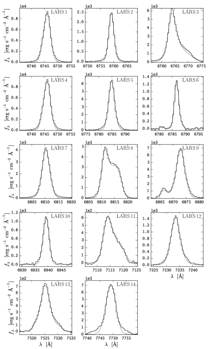
Figure 3: Integrated continuum-subtracted H$\alpha$ profiles of the LARS galaxies (black) compared to summed 1D Gaussian model profiles (grey) from which radial-velocity and velocity-dispersion maps were generated.

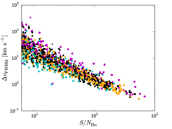
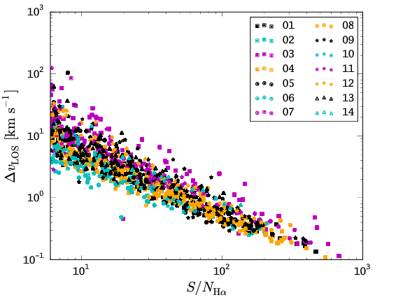
Figure 4: Uncertainties on derived velocity dispersions (left panel) and radial velocities (right panel) for Gaussian profile fits to H$\alpha$ for all galaxies. All uncertainties for a specific galaxy have the same symbol according to the legend in the right panel.

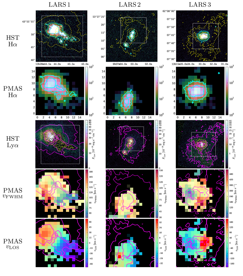
Figure 5: Comparison of LARS HST imaging results of the LARS sample to spatially resolved PMAS H$\alpha$ spectroscopy. North is always up and east is always to the left. For each galaxy from top to bottom: The first panel shows the LaXs H$\alpha$ line intensity map; tick labels indicate right-ascension and declination and an asinh-scaling is used cut at 95% of the maximum value. The second panel shows a SNR map of the continuum-subtracted H$\alpha$ signal observed with PMAS. Tick labels in the PMAS SNR map are in arc-seconds, the scaling is logarithmic from 1 to $10^{3}$ and only spaxels with $S/N>1$ are shown. The third panel shows the LARS Ly$\alpha$ images with a colourbar indicating the flux scale in cgs-units; scaling is the same as in the H$\alpha$ map. The fourth panel shows resolution-corrected H$\alpha$ $v_{\mathrm{FWHM}}$ maps from our PMAS observations and the corresponding H$\alpha$ $v_{\mathrm{LOS}}$ maps are displayed in the fifth panel. In the first and third panel we indicate position and extend of the PMAS field of view with a white box. Cyan contours in the HST H$\alpha$ image are contours of constant surface brightness, adjusted to highlight the most prominent morphological features. Similarly, magenta contours in the HST Ly$\alpha$ images indicate the Ly$\alpha$ morphology; these contours are also shown in the fourth and fifth panel. To highlight the difference between Ly$\alpha$ and H$\alpha$, the Ly$\alpha$ and H$\alpha$ panels contain as dashed yellow lines the contours from the H$\alpha$ and Ly$\alpha$ panels, respectively.

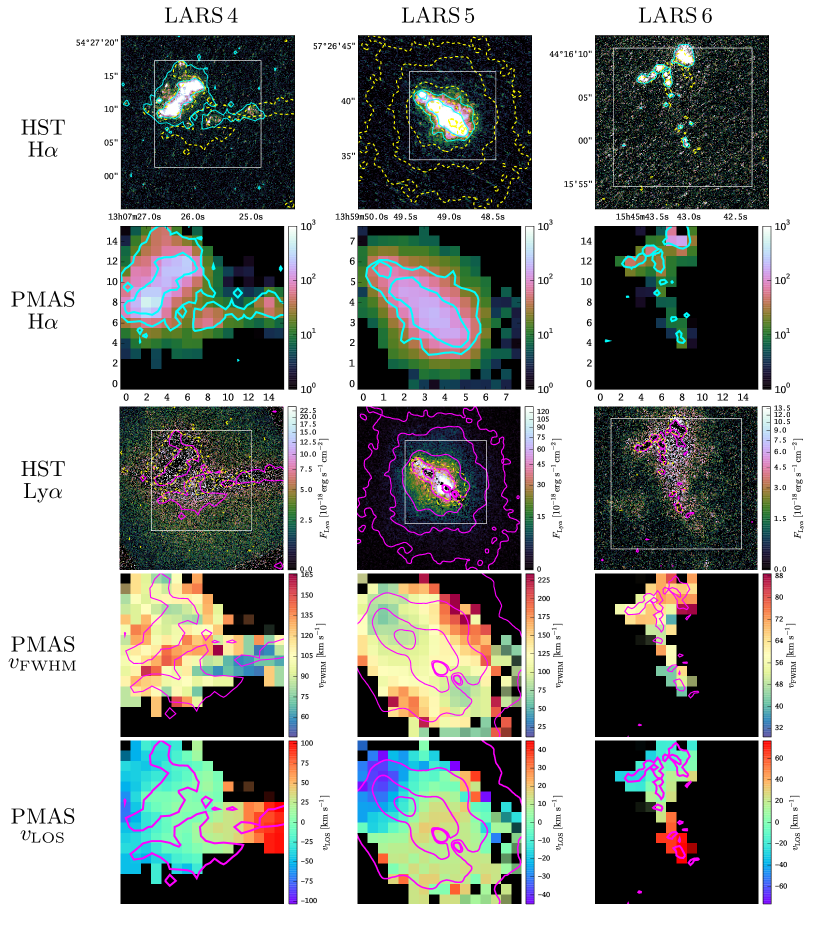
Figure 5: Continued.

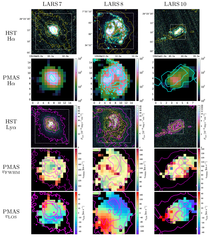
Figure 5: Continued.

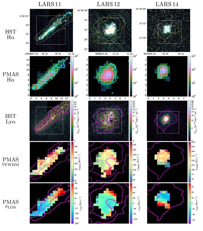
Figure 5: Continued.

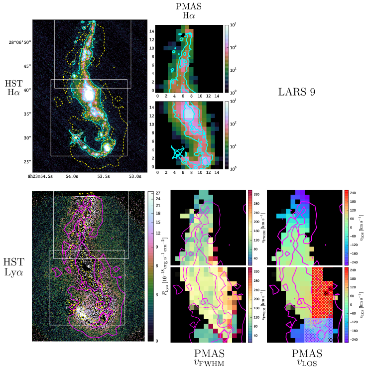
Figure 6: Comparison of LARS HST imaging results to spatially resolved PMAS H$\alpha$ spectroscopy for LARS 9. For detailed description of individual panels see caption of Figure 5. This galaxy was covered with 2 PMAS pointings. Hatched regions in the $v_{\mathrm{LOS}}$ map indicate regions, where the H$\alpha$ emission shows a more complex profile that could not be described by a simple Gaussian (cf. Appendix A.9).

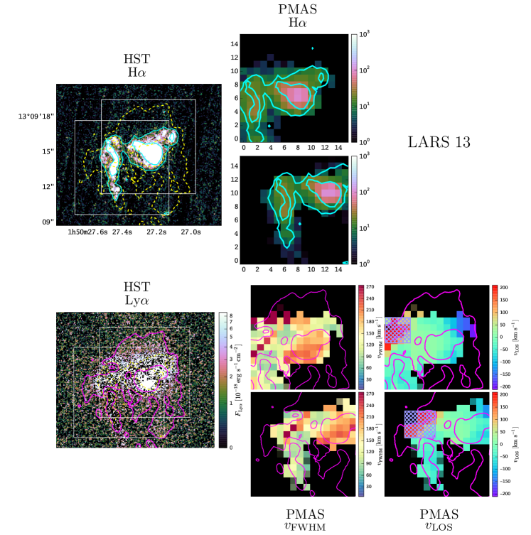
Figure 7: Same as Figure 6, but for LARS 13. Hatched region in the $v_{\mathrm{LOS}}$ map indicates the region, where the H$\alpha$ emission shows a more complex profile that could not be described by a simple Gaussian (cf. Appendix A.13).

We condense the kinematical information traced by H$\alpha$ in our data cubes into two-dimensional maps depicting velocity dispersion and line of sight radial-velocity at each spaxel. Both quantities are derived from 1D Gaussian fits to the observed line shapes from the continuum subtracted cube (see Sect. 3.4). We calculate the radial velocity offset $v_{\mathrm{LOS}}$ to the central wavelength value given by the mean of all fits and the FWHM of the fitted line in velocity space $v_{\mathrm{FWHM}}$. To obtain higher signal to noise ratios in the galaxies’ outskirts we use the weighted Voronoi tessellation binning algorithm by Diehl & Statler (2006), which is a generalisation of the Voronoi binning algorithm of Cappellari & Copin (2003).

We visually scrutinised the fits to the spectra and decided that lines observed at a SNR of 6 were still reliably fit. Hence, 6 defines the minimum SNR in the Voronoi binning algorithm. Furthermore, we adopted a maximum bin size of 3$\times$3 pixels. In those calculations signal and noise are defined as in Sect. 3.4. In what follows, only results from the fits to bins that meet the minimum signal to noise requirement are considered. Most of the bins used are actually only a single spaxel, and very few bins in the outskirts of the galaxies meeting the minimum SNR criterion consist of 2 or 3 spaxels. In practice this means that we are typically sensitive to regions at H$\alpha$ surface brightness higher than $5\times 10^{-16}$erg s^-1cm^-2arcsec^-2. Using the Kennicutt (1998) conversion and neglecting extinction, this translates to an detection limit of $\sim 3\times 10^{-2}$M_⊙yr^-1kpc^-1, more than an order of magnitude deeper than probed by high redshift integral field spectroscopy studies ($\sim 1$M_⊙yr^-1kpc^-1, see e.g. Law et al. 2009).

By visual inspection we also ensured that 1D Gaussian profiles are a sufficient model of the observed H$\alpha$ profiles seen in the PMAS LARS data cubes. Only in two galaxies (LARS 9 and LARS 13) we have some spaxels where a 1D Gaussian certainly fails to reproduce the complexity of the observed spectral shape. Moreover, in LARS 14 weak broad wings are visible in the individual H$\alpha$ profiles. We have not attempted to model these special cases, but we describe their qualitative appearance in detail in the Appendices A.9, A.13 and A.14 and acknowledge their existence in our interpretation in Sect. 6. To demonstrate the overall quality of our H$\alpha$ velocity fields, we compare in Fig. 3 the integrated H$\alpha$ profiles of the LARS galaxies to the sum of the fitted 1D Gaussians used to generate the $v_{\mathrm{FWHM}}$ and $v_{\mathrm{LOS}}$ maps. As can be seen the observed profile and the one derived from the models are largely in agreement. The strongest deviation between data and models is apparent in LARS 14, where the broad wings of the observed H$\alpha$ profile are not reproduced at all by out 1D Gaussian models (cf. Sect. 6.1 and Appendix A.14).

To estimate formal uncertainties on $v_{\mathrm{FWHM}}$ and $v_{\mathrm{LOS}}$, we use a Monte Carlo technique: We perturb our spectra 100 times with the noise from our noise cubes and then fit the 1D Gaussian profile in exactly the same way to each of these 100 realisations. The width of the distribution of all fit results characterised by their standard deviation gives a robust measure for the uncertainty on the derived quantities (see also Appendix B.4. in Davies et al. 2011). The central moment of the distribution is the final value that will be shown in our maps. In Fig. 4 we display for all performed fits the error on the velocity dispersion $\Delta v_{\mathrm{FWHM}}$ and on radial velocity $\Delta v_{\mathrm{LOS}}$ as a function of the lines SNR. We note, that on average our uncertainties on $v_{\mathrm{FWHM}}$ and $v_{\mathrm{LOS}}$ follow the scaling laws expected for fitting Gaussian profiles to noisy emission-line spectra $\Delta v_{\mathrm{LOS}}\propto\Delta v_{\mathrm{FWHM}}\propto v_{\mathrm{FWHM}}^{1/2}\mathrm{SNR}^{-1}$ (Landman et al. 1982; Lenz & Ayres 1992). For reference, at our minimum $\mathrm{SNR}=6$ we have typical errors of $\Delta v_{\mathrm{FWHM}}\approx 30\,$km s^-1 and $\Delta v_{\mathrm{LOS}}\approx 10\,$km s^-1, and at the median (mean) SNR of our data - $\mathrm{SNR}_{\mathrm{median}}=22$ ($\mathrm{SNR}_{\mathrm{mean}}=50$) - we have $\Delta v_{\mathrm{FWHM}}\approx 7\,$km s^-1 ($\approx 3\,$km s^-1) and $\Delta v_{\mathrm{LOS}}\approx 3\,$km s^-1 ($\approx 1\,$km s^-1).

In Fig. 5 we show the resulting $v_{\mathrm{FWHM}}$ and $v_{\mathrm{LOS}}$ maps together with the LaXs Ly$\alpha$ images (lower three panels). Maps and images of the galaxies observed with two pointings are shown in Fig. 6 and Fig. 7 for LARS 9 and LARS 13, respectively. All $v_{\mathrm{FWHM}}$ maps have been corrected for instrumental broadening using the spectral resolving power maps derived in Sect. 3.3. In all $v_{\mathrm{LOS}}$ and $v_{\mathrm{FWHM}}$ panels we overlay contours derived from the Ly$\alpha$ image to emphasise distinctive morphological Ly$\alpha$ properties.

Individual maps are discussed in Appendix A. Using the classification scheme introduced by Flores et al. (2006) (see also Sect. 3.3 in Glazebrook 2013) the LARS galaxies can be characterised by the qualitative appearance of their velocity fields:

• Rotating Disks: LARS 8 and LARS 11. Both galaxies show a regular symmetric dipolar velocity field with a steep gradient in the central regions. This steep gradient is also the reason for artificially broadened emission near the kinematical centre. Morphologically both galaxies also bear resemblance to a disk and the kinematical axis is aligned with the morphological axis. However, we point out in Appendix A.8 that LARS 8 can also be classified as a shell galaxy, hinting at a recent merger event.

• Perturbed Rotators: LARS 1, LARS 3, LARS 5, LARS 7, and LARS 10. In those galaxies traces of orbital motion are still noticeable, but the maps look either significantly perturbed compared to a classical disk case (LARS 3, LARS 5, LARS 7 and LARS 10) and/or the observed velocity gradient is very weak (LARS 1, LARS 5 and LARS 10). Based solely on morphology, we previously classified two of those galaxies as dwarf edge-on disks (LARS 5 and LARS 7 - ; , ). Moreover, LARS 3 is a member of a well known merger of two similar massive disks (cf. Appendix  A.3). From our imaging data alone LARS 7 and LARS 10 bear resemblance to shell galaxies (cf. Appendices A.7 and A.10).

• Complex Kinematics: LARS 2, LARS 4, LARS 6, LARS 9, LARS 12 LARS 13, and LARS 14. These seven galaxies are characterised by more chaotic $v_{\mathrm{LOS}}$ maps and they all have also irregular morphologies. Four of the irregulars consist of photometrically well separated components that are also kinematically distinct (LARS 4, LARS 6, LARS13 and LARS 14), while the other three each have their own individual peculiarities (LARS 2, LARS 9 and most spectacularly LARS 12 - cf. Appendices  A.2, A.9 and A.12).

These kinematic classes are also listed in Table 10.

Notably, in all LARS galaxies, except for LARS 6, we observe high-velocity dispersions ($v_{\mathrm{FWHM}}\gtrsim 100$ km s^-1); the most extreme case is LARS 3 where locally lines as broad as $v_{\mathrm{FWHM}}\sim 400$ km s^-1 are found. The observed width of the H$\alpha$ line seen in our $v_{\mathrm{FWHM}}$ maps can be described as a successive convolution of the natural H$\alpha$ line (7 km s^-1 FHWM) with the thermal velocity distribution of the ionised gas (21.4 km s^-1 FWHM at 10⁴K) and with non-thermal motions in the gas (e.g. Jiménez-Vicente et al. 1999). Since all our dispersion measurements are significantly higher than the thermally broadened profile non-thermal motions dominate the observed line-widths. Non-thermal motions could be centre-to-centre dispersions of the individual H ii regions and turbulent motions of the ionised gas. The latter appears to be the main driver for the observed line widths, since the observed velocity dispersions are highly supersonic (i.e. $\gtrsim 10$ km s^-1 for H ii at 10⁴K, see also Sect. 5.1 in Glazebrook 2013).

5.2 Global kinematical properties: $v_{\mathrm{shear}}$, $\sigma_{0}$, $\sigma_{\mathrm{tot}}$ and $v_{\mathrm{shear}}/\sigma_{0}$

Table 2: Global kinematic parameters from H$\alpha$ for the LARS galaxies, calculated as described in Sect. 5.2. For reference we also tabulate $\mathrm{EW}_{\mathrm{Ly\alpha}}$, Ly$\alpha$/H$\alpha$ and $f_{\mathrm{esc.}}^{\mathrm{Ly\alpha}}$ from Paper II, as well as $\xi_{\mathrm{Ly\alpha}}$ from Hayes et al. (2013).

ID	Class	$\sigma_{\mathrm{0}}$	$\sigma_{\mathrm{tot}}$	$v_{\mathrm{shear}}$	$v_{\mathrm{shear}}/\sigma_{\mathrm{0}}$	$\mathrm{EW}_{Ly\alpha}$	Ly$\alpha$/H$\alpha$	$f_{\mathrm{esc.}}^{\mathrm{Ly\alpha}}$	$\xi_{\mathrm{Ly\alpha}}$
		[km s-1]	[km s-1]	[km s-1]		[Å]
1	P	47.5$\,\pm\,$0.1	160.5	156$\,\pm\,$2	1.2$\,\pm\,$0.1	33.0	1.36	0.119	3.37
2	C	38.6$\,\pm\,$0.9	146.0	123$\,\pm\,$3	0.6$\,\pm\,$0.1	81.7	4.53	0.521	2.27
3	P	99.5$\,\pm\,$3.7	130.9	138$\,\pm\,$3	1.4$\,\pm\,$0.2	16.3	0.16	0.003	0.77
4	C	44.1$\,\pm\,$0.1	155.1	174$\,\pm\,$9	1.7$\,\pm\,$0.1	0.00	0.00	0.000	…
5	P	46.8$\,\pm\,$0.3	154.7	137$\,\pm\,$4	0.8$\,\pm\,$0.1	35.9	2.16	0.174	2.61
6	C	27.2$\,\pm\,$0.3	158.9	152$\,\pm\,$7	1.9$\,\pm\,$0.2	0.00	0.00	0.000	…
7	P	58.7$\,\pm\,$0.3	167.4	131$\,\pm\,$3	0.5$\,\pm\,$0.1	40.9	1.94	0.100	3.37
8	R	49.0$\,\pm\,$0.1	111.8	155$\,\pm\,$3	3.2$\,\pm\,$0.1	22.3	0.67	0.025	1.12
9	C	58.6$\,\pm\,$0.1	112.7	182$\,\pm\,$3	3.1$\,\pm\,$0.1	3.31	0.13	0.007	$>$2.85
10	P	38.2$\,\pm\,$1.0	149.2	136$\,\pm\,$3	0.9$\,\pm\,$0.2	8.90	0.47	0.026	2.08
11	R	69.3$\,\pm\,$3.8	114.8	149$\,\pm\,$4	2.1$\,\pm\,$0.3	7.38	0.72	0.036	2.27
12	C	72.7$\,\pm\,$1.0	181.3	196$\,\pm\,$3	1.3$\,\pm\,$0.1	8.49	0.48	0.009	3.48
13	C	69.2$\,\pm\,$0.7	197.3	183$\,\pm\,$4	2.5$\,\pm\,$0.2	6.06	0.29	0.010	1.74
14	C	67.3$\,\pm\,$1.3	172.9	140$\,\pm\,$1	0.6$\,\pm\,$0.1	39.4	2.24	0.163	3.62

We now quantify the global kinematical properties of our H$\alpha$ velocity fields that were qualitatively discussed in the previous section. Therefore we compute three non-parametric estimators that are commonly adopted in the literature for this purpose (e.g. Law et al. 2009; Basu-Zych et al. 2009; Green et al. 2010; Glazebrook 2013; Gonçalves et al. 2010; Green et al. 2014; Wisnioski et al. 2015): Shearing velocity $v_{\mathrm{shear}}$, intrinsic velocity dispersion $\sigma_{0}$ and their ratio $v_{\mathrm{shear}}/\sigma_{0}$. We describe the physical meaning of those parameters and our method to determine them in the following three subsections. Furthermore, we also calculate the integrated velocity dispersion $\sigma_{\mathrm{tot}}$. This measure provides a useful comparison for unresolved distant galaxies (cf. Sect. 5.2.4). Our results on $v_{\mathrm{shear}}$, $\sigma_{0}$, $\sigma_{\mathrm{tot}}$ and $v_{\mathrm{shear}}/\sigma_{0}$ are tabulated in Table 10.

5.2.1 Shearing velocity $v_{\mathrm{shear}}$

The shearing velocity $v_{\mathrm{shear}}$ is a measure for the large-scale gas bulk motion along the line of sight. We calculate it via

$$v_{\mathrm{shear}}=\frac{1}{2}\left(v_{\mathrm{max}}-v_{\mathrm{min}}\right)\;\text{.}$$ (1)

Here we take the median of the lower and upper 5 percentile of the distribution of values in the $v_{\mathrm{LOS}}$ maps for $v_{\mathrm{min}}$ and $v_{\mathrm{max}}$, respectively. This choice ensures that the calculation is robust against outliers while sampling the true extremes of the distribution. We conservatively estimate the uncertainty by propagating the full width of the upper and lower 5 percentile of the velocity map. We list our results for $v_{\mathrm{shear}}$ in the second column of Table 10. Our derived $v_{\mathrm{shear}}$ values for the LARS sample range from $30$ km s^-1 to $180$ km s^-1, with 65 km s^-1 being the median. This is less than half the typical maximum velocity $v_{\mathrm{max}}$ of H$\alpha$ rotation curves observed in spiral galaxies - e.g. $v_{\mathrm{max}}=145$ km s^-1 is the median of 153 local spirals (Epinat et al. 2010). In contrast to our $v_{\mathrm{shear}}$ measurement, $v_{\mathrm{max}}$ values are inclination corrected. In a sample with random inclinations on average the correction $v_{\mathrm{shear}}=\frac{\pi}{4}v_{\mathrm{max}}\approx 0.79\,v_{\mathrm{max}}$ is expected (e.g. Law et al. 2009) but even with this correction classical disks appear still incompatible with most of our measurements by a factor larger than two. Only for the two galaxies that we classified as rotating disks in Sect. 5.1 we find $v_{\mathrm{shear}}$ values compatible with local rotators. Nevertheless, high $v_{\mathrm{shear}}$ values do not necessarily imply the presence of a disk. Large-scale bulk motions at high amplitude occur also in close encounters of spatially and kinematically distinct companions (e.g. LARS 13).

Sensitivity is an important factor in the determination of the observed $v_{\mathrm{shear}}$. An observation of less depth will not detect fainter regions at larger radii, which may have the highest velocities. Indeed, for most of our galaxies the spatial positions of $v_{\mathrm{min}}$ and $v_{\mathrm{max}}$ values are in those outer lower surface-brightness regions. Hence observations of lower sensitivity will be biased to lower $v_{\mathrm{shear}}$ values. This sensitivity bias is strongly affecting high-$z$ studies because such observations often limited only to the brightest regions (Law et al. 2009; Gonçalves et al. 2010).

5.2.2 Intrinsic velocity dispersion $\sigma_{0}$

The intrinsic velocity dispersion $\sigma_{0}$ (sometimes also called resolved velocity dispersion or local velocity dispersion, cf. Glazebrook 2013, Sect. 1.2.1) is in our case a measure for the typical random motions of the ionised gas within a galaxy. We calculate it by taking the flux weighted average of the observed velocity dispersions in all spaxels:

$$\sigma_{0}=\frac{\sum F^{\mathrm{H\alpha}}_{\mathrm{spaxel}}\sigma_{\mathrm{spaxel}}}{\sum F^{\mathrm{H\alpha}}_{\mathrm{spaxel}}}\;\text{.}$$ (2)

Here $F^{\mathrm{H\alpha}}_{\mathrm{spaxel}}$ is the H$\alpha$ flux in each spaxel and $\sigma_{\mathrm{spaxel}}$ is the velocity dispersion measured in that spaxel; the sum runs over all spaxels with $\text{SNR}\geq 6$ (Sect. 5.1). Such a flux-weighted summation $\sigma_{0}$ has been widely adopted in the literature to quantify the typical intrinsic velocity dispersion component (e.g. Östlin et al. 2001; Law et al. 2009; Gonçalves et al. 2010; Green et al. 2010; Glazebrook 2013; Green et al. 2014).

PSF smearing in the presence of strong velocity gradients broadens the H$\alpha$ line at the position of the gradients. Such a broadening could bias our calculation of the intrinsic velocity dispersion. At the distances of the LARS galaxies our typical seeing-disk PSF FWHM of 1″ corresponds to scales of 0.6 kpc to 3 kpc. In most of our observations this average PSF FWHM is comparable to the size of one PMAS spaxel (1″$\times$1″) and most of the LARS galaxies exhibit rather weak velocity gradients. The PSF smearing effect is seen only in galaxies with strong velocity gradients (e.g. LARS 8, cf. Appendix  A.8), especially when observed with PMAS’ 0.5″$\times$0.5″ magnification mode (e.g. LARS 12, cf. Appendix A.12). In principle the effect could be corrected by subtracting a PSF-smeared kinematical model of the $v_{\mathrm{LOS}}$ velocity field. Given the complexity of our observed velocity fields, however, this is not practicable. And, moreover, at $z\sim 0.1$ Green et al. (2014) find that for classical rotating disk kinematics the velocity dispersions corrected by a kinematical model are, on average, negligible. Comparison between adaptive-optics derived PSF-smearing unaffected $\sigma_{0}$ values to those derived from seeing-limited observations were presented by Bassett et al. (2014). They find that while for one galaxy $\sigma_{0}$ remains unaffected by an increase in spatial resolution, for the other galaxy $\sigma_{0}$ decreases by $\sim$10 km s^-1. Bassett et al. (2014) attribute the $\sim$10 km s^-1 discrepancy in one of their galaxies to a strong velocity gradient that is co-spatial with the strongest emission. A similar comparison is possible for three of our LARS galaxies - LARS 12, LARS 13 and LARS 14. For these galaxies adaptive optics IFS observations were presented by Gonçalves et al. (2010) (see Appendices A.12, A.13 and A.14). Gonçalves et al. (2010) derive $\sigma_{0}=67$ km s^-1, $\sigma_{0}=74$ km s^-1 and $\sigma_{0}=71$ km s^-1 for LARS 12, LARS 13 and LARS 14, respectively. These values are in agreement with our measurements of $\sigma_{0}=73$ km s^-1, $\sigma_{0}=69$ km s^-1 and $\sigma_{0}=67$ km s^-1 for those galaxies. From all these considerations we are certain, that the adopted formalism in Eq. (2) gives a robust estimate of the intrinsic velocity dispersion.

We list our derived values for $\sigma_{0}$ in the third column of Table 10. In general, the ionised gas kinematics of the LARS galaxies are characterised by high intrinsic velocity dispersions ranging from 40 km s^-1 to 100 km s^-1 with 54 km s^-1 being the median of the sample. Such high intrinsic dispersions are in contrast to H ii velocity dispersions of $\sim 10-50$ km s^-1 typically found in local spirals (e.g. Epinat et al. 2008a, b, 2010; Erroz-Ferrer et al. 2015). In high-$z$ star-forming galaxies intrinsic dispersions $\gtrsim 50$ km s^-1 appear to be the norm (e.g. Puech et al. 2006; Genzel et al. 2006; Law et al. 2009; Förster Schreiber et al. 2009; Erb et al. 2014; Wisnioski et al. 2015). In the local $z\lesssim 0.1$ Universe high intrinsic velocity dispersions are also found in the studies of blue compact galaxies (BCGs, Östlin et al. 1999, 2001), local Lyman break analogues (Basu-Zych et al. 2009; Gonçalves et al. 2010) and (ultra-)luminous infrared galaxies (e.g Monreal-Ibero et al. 2010). Finally, $\sigma_{0}$ values of comparable amplitude are also common in a sample of 67 bright H$\alpha$ emitters ($10^{40.6}\leq L_{\mathrm{H\alpha}}\leq 10^{42.6}$) (Green et al. 2010, 2014). Indeed, Green et al. (2010) and Green et al. (2014) show that star formation rate is positively correlated with intrinsic velocity dispersion. We will confirm this trend among our LARS galaxies and discuss its implications on Ly$\alpha$ observables in Sect. 6.3.

5.2.3 $v_{\mathrm{shear}}/\sigma_{0}$ ratio

The ratio $v_{\mathrm{shear}}/\sigma_{0}$ is a metric to quantify whether the gas kinematics are dominated by turbulent or ordered (in some cases orbital) motions. Our results for this quantity are listed in Table 10. Given the above (Sects. 5.2.1 and 5.2.2) mentioned differences to disks, it appears cogent that our $v_{\mathrm{shear}}/\sigma_{0}$ ratios (median 1.4, mean 1.6) are much smaller than typical disk $v_{\mathrm{shear}}/\sigma_{0}$ ratios $\sim 4-8$ (first to last quartile of the Epinat et al. sample).

Objects with $v_{\mathrm{shear}}/\sigma_{0}<1$ are commonly labelled dispersion dominated galaxies (Newman et al. 2013; Glazebrook 2013). - According to this criterion five galaxies of the 14 LARS sample are dispersion dominated: LARS 2, LARS 5, LARS 7, LARS 10 and LARS 14 - three perturbed rotators and two with complex kinematics. Dispersion dominated galaxies are frequently found in kinematic studies of high-$z$ star forming galaxies. Local samples with a similar high fraction ($\sim 35$%) of dispersion dominated galaxies are the blue compact galaxies studied by Östlin et al. (2001) or the Lyman break analogues studied by Gonçalves et al. (2010) . In Sect. 6.3 we will show that dispersion dominated systems are more likely to have a significant fraction of Ly$\alpha$ photons escaping.

5.2.4 Integrated velocity dispersion $\sigma_{\mathrm{tot}}$

For reference we also compute the integrated (spatially averaged) velocity dispersion $\sigma_{\mathrm{tot}}$. This measure provides a useful comparison for studies of unresolved distant galaxies, where no disentanglement between ordered and disordered, random motions is possible (e.g. McLinden et al. 2011; Guaita et al. 2013; McLinden et al. 2014; Rhoads et al. 2014; Erb et al. 2014).

We obtain $\sigma_{\mathrm{tot}}$ by calculating the square root of the second moment of the integrated H$\alpha$ profiles shown in Fig. 3. The results are given in the fourth column of Table 10. Our integrated velocity dispersions for the LARS sample range from 46 km s^-1 to 115 km s^-1, with 70 km s^-1 being the median of the sample. Given the high SNR of the integrated profiles the formal uncertainties on this $\sigma_{\mathrm{tot}}$ are very small ($\sim 10^{-2}$km s^-1). As expected, when large scale motions dominate in the integrated spectrum (i.e. high $v_{\mathrm{shear}}/\sigma_{0}$ ratios), $\sigma_{\mathrm{tot}}$ is significantly larger than $\sigma_{0}$, but for dispersion dominated systems the discrepancy becomes less extreme.

6 Discussion: Influence of H$\alpha$ kinematics on a galaxy’s Ly$\alpha$ emission

6.1 Clues on Ly$\alpha$ escape mechanisms via spatially resolved H$\alpha$ kinematics

Recent theoretical modelling of the Ly$\alpha$ radiative transport within realistic interstellar medium environments predicts that small scale interstellar medium physics are an decisive factor in regulating the Ly$\alpha$ escape from galaxies (Verhamme et al. 2012; Behrens & Braun 2014). In particular Behrens & Braun (2014) demonstrate how supernova blown outflow cavities become favoured escape channels for Ly$\alpha$ radiation. These cavities naturally occur in zones of enhanced star formation activity, where the input of kinetic energy from supernovae and stellar winds into the surrounding interstellar medium is also expected to drive highly turbulent gas flows. Do we see supporting evidence for this scenario in our IFS observations of the LARS galaxies?

As described in Sect. 5.1, all our velocity fields are characterised by broad profiles that are best explained by turbulent flows of ionised gas. The more violent these flows are, the more likely they carve holes or bubbles through the interstellar medium through which the ionised gas eventually flows out into the galaxy’s halo. Close inspection of Fig. 5 reveals, that in LARS 1, LARS 3 and LARS 13 (Fig. 7) zones of high Ly$\alpha$ surface brightness occur near or even cospatial to zones where for these galaxies the maximum velocity dispersions are observed. In both LARS 1 and LARS 13 these zones are also co-spatial with the regions of highest H$\alpha$ surface-brightness, hence here the star formation rate density is highest. Moreover, in LARS 1 the H$\alpha$ image shows a diffuse fan-like structure emanating outwards from this star-forming knot ( ; , ). Finally, also the analysis of the COS spectra in Paper V shows blue-shifted low-ionisation state interstellar absorption lines in LARS 1 and LARS 13 indicative of outflowing neutral gas. Hence for those two galaxies together with the high-resolution HST imaging data our IFS data provides further evidence for the relevance of localised outflows in shaping the observed Ly$\alpha$ morphology.

However, already in LARS 3 the interpretation is not as straight-forward. Here the broadest H$\alpha$ lines do not occur co-spatial with the highest star formation rate density. Although also here the COS spectrum shows a bulk outflow of cold neutral gas (Rivera-Thorsen et al. 2015), the locally enhanced dispersion values seen in the PMAS maps appear not to be related to this outflow. Instead, it appears more naturally that the high turbulence within the ionised gas is not primarily driven by star formation activity, but is rather the result of the violent interaction with the north-western companion (see e.g. Teyssier et al. 2010 for theoretical support). The interpretation is further complicated by the fact, that the HST imaging data resolves the local Ly$\alpha$ knot on smaller scales then which we are probing with our PMAS observations.

Nevertheless, there is another example among the LARS galaxies for Ly$\alpha$ escape being related to an outflow: LARS 5 (cf. Duval, A&A submitted). For this galaxy we presumed already in Paper II the existence of a starburst driven wind based solely on the filamentary structure seen in the HST H$\alpha$ image. Our dispersion map now reveals that these filaments fill the interior of a biconical structure, with its base confined on the most prominent star-forming clump (cf. Appendix A.5) – fully in accordance with theoretical expectations for an evolved starburst driven superwind (e.g. Cooper et al. 2008). Also here Ly$\alpha$ photons could preferentially escape the disc through the cavity blown by the wind. The strongest Ly$\alpha$ enhancement is found directly above and below the main star-forming clump and the low surface brightness Ly$\alpha$ halo is then produced by those photons scattering on a bipolar shell-like structure of ambient neutral gas swept up by the superwind. Unfortunately, the brightest hot-spots in Ly$\alpha$ above and below the plane are at the base of this outflowing cone and occur at scales that we cannot resolve in our PMAS data. Similar but less spectacular examples of elevated velocity dispersions above and below a disk can be seen in LARS 7 and LARS 11, with both galaxies are also being embedded in low-surface brightness Ly$\alpha$ halos.

Another possible example for the importance of outflow kinematics in facilitating direct Ly$\alpha$ escape is the most luminous LAE in the sample: LARS 14 (cf. Appendix A.14). Here the observed H$\alpha$ profiles are always characterised by an underlying fainter broad component (see Fig. 3) that is believed to be directly related to outflowing material (e.g. Yang et al. 2015).

We conclude that while in some individual cases a causal connection between spatially resolved H$\alpha$ kinematics and localised outflow scenarios might be conjectured, globally this is not a trend seen in our observations. We note further, that H$\alpha$ kinematics tell only one part of the whole story, and the suggested outflow scenarios should also be traceable by gas with a high degree of ionisation. At least for one galaxy with Ly$\alpha$ imaging similar to the LARS galaxies, such a connection has been demonstrated: ESO338-IG04. Recently, Bik et al. (2015) analysed observations of this galaxy obtained with the MUSE integral field spectrograph (Bacon et al. 2014). They show, that the Ly$\alpha$ fuzz seen around the main star-forming knot of this galaxy (Hayes et al. 2005; Östlin et al. 2009) can be related to an outflow which can be traced both with H$\alpha$ kinematics and by a high degree of ionisation. As a difference to our observations, Bik et al. (2015) see the fast outflowing material in their $v_{\mathrm{LOS}}$ map as significantly redshifted H$\alpha$ emission. No similar prominent effect is apparent in our $v_{\mathrm{LOS}}$ maps. Nevertheless, the $v_{\mathrm{LOS}}$ fields of LARS 7 and LARS 12 display strongly localised redshifts in H$\alpha$ that are spatially coincident with filamentary H$\alpha$ fingers, hence here we might see also a fast outflow pointed away from the observer. But also in those galaxies, no co-spatial relation between Ly$\alpha$ emissivity and the suspected outflows can be established.

6.2 Comparison of H$\alpha$ to H i observations

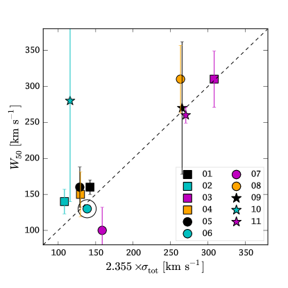
Figure 8: Comparison of integrated H i linewidth $W_{50}$ to FWHM of the H$\alpha$ integrated velocity dispersion $2\sqrt{2\ln 2}\times\sigma_{\mathrm{tot}}$. The dashed line indicates the one-to-one relation. We note, that for LARS 6 (encircled point) we plot as $W_{50}$ a preliminary result based upon VLA C-configuration interferometry, as the beam of the GBT profile (used to derive $W_{\mathrm{50}}$ in Paper III) is too broad to separate LARS 6 from a neighbouring galaxy.

Radiative transfer of Ly$\alpha$ photons depends on the relative velocity differences between scattering H i atoms and Ly$\alpha$ sources. If the Ly$\alpha$ sources are out of resonance with the bulk of the neutral medium, they are less likely scattered, and in turn more likely to escape the galaxy. It is exactly this interplay between the ionised and neutral ISM phases that is determining the whole the Ly$\alpha$ radiative transfer. In Paper III we studied LARS galaxies in the H i 21 cm line, using single-dish GBT and VLA D-configuration observations (cf. Sect. 4). We now attempt a comparison between the neutral and ionised gas kinematics in the LARS galaxies, cognisant of the fact that the spatial scales probed by both instruments are much larger than our PMAS H ii observations.

Generally our GBT H i spectra have low SNR, and for the three most distant LARS galaxies – LARS 12, LARS 13 and LARS 14 – we could not detect any significant signal at all. The profiles are mostly single- or multiple-peaked, but rarely show a classical double-horn profile that would be expected for a flat rotation curve. Hence, qualitatively our observed GBT H i line profiles are consistent with our PMAS results that most of the LARS galaxies are kinematically perturbed or sometimes even strongly interacting systems.

In Paper III we measured the width of the H i lines at 50% of the line peak from the GBT spectra. In Fig. 8 we compare this quantity, $W_{50}$, to the FWHM of the integrated H$\alpha$ velocity dispersion $\sigma_{\mathrm{tot}}$ (Sect. 5.2.4). Notably, two systems deviate significantly from the one-to-one relation: LARS 7 and LARS 10. LARS 10 shows the lowest SNR H i spectrum and moreover our PMAS FoV does not capture two smaller star-forming clumps in the south-east. Therefore we believe that observational difficulties are source for the $\sigma_{\mathrm{tot}}$–$W_{50}$ difference in this galaxy. In LARS 7, however, we suspect the difference to be genuine. In this galaxy the H$\alpha$ morphology is significantly puffed up and rounder compared to the disk-like continuum (cf. Appendix A.7). Therefore we suspect that the smaller $W_{50}$ measurement indicates that bulk of H i is in a kinematically more quiescent state then the ionised gas. This galaxy is one of the stronger LAEs in the sample ($f_{\mathrm{esc.}}^{\mathrm{Ly\alpha}}=0.14$ and EW_Lyα=40Å). That considerable amounts of Ly$\alpha$ photons escape from LARS 7 was noted as peculiar in Paper V, since the metal absorption lines indicated large amounts of neutral gas sitting at the systemic velocity of the galaxy. Our observations now indicate that the intrinsic Ly$\alpha$ photons are produced in gas that is less quiescent than the scattering medium, which therefore is more transparent for a significant fraction of the intrinsic Ly$\alpha$ photons.

Spatially resolved VLA velocity fields are available for only a subset of five LARS galaxies (LARS 2, LARS 3, LARS 4, LARS 8, LARS 9). They represent rotations, disturbed by interactions with neighbours. In four of them, H i kinematical axes have similar orientations as those of the PMAS H$\alpha$ velocity field. In the fifth object, the complex interacting system LARS 9, the H$\alpha$ and H i velocity fields show different characteristics, but the complexities seen in the PMAS maps of this galaxy are on scales far beyond the resolving power of the VLA D-configuration (cf. Appendix A.9). However, some of the LARS galaxies have already been observed with the VLA in C- and B-configuration and the analysis is currently in progress. These data will allow for the first time a comparison between H$\alpha$, H i and Ly$\alpha$ on meaningful physical scales. It is evident, that these comparisons will provide a critical benchmark for our understanding of Ly$\alpha$ radiative transfer in interstellar and circum-galactic environments.

6.3 Relations between kinematical properties and galaxy parameters

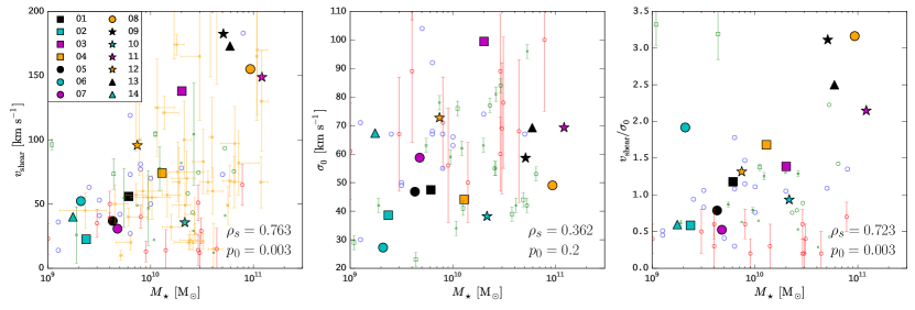
Figure 9: Global H$\alpha$ kinematical parameters $v_{\mathrm{shear}}$ (left panel), $\sigma_{0}$ (middle panel) and $v_{\mathrm{shear}}/\sigma_{0}$ (right panel) in comparison to stellar mass for LARS galaxies (from Hayes et al. 2014) and in comparison to literature values: DYNAMO $z\sim 0.1$ [compact] perturbed rotators from Green et al. (2014) as [small] green circles; DYNAMO $z\sim 0.1$ [compact] complex kinematics from Green et al. (2014) as [small] green squares; Local Lyman Break Analogues from Gonçalves et al. (2010) as blue circles; Keck/OSIRIS resolved $z\sim 2-3$ star forming galaxies from Law et al. (2009) as red circles; SINS $z\sim 2-3$ galaxies from Förster Schreiber et al. (2009) as orange squares (only in the left panel). Uncertainties given where available. The LARS galaxies are represented by symbols according to the legend in the left panel. Spearman rank correlation coefficients $\rho_{s}$ and corresponding $p_{0}$ values for the LARS galaxies are shown in each panel.

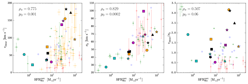
Figure 10: Global H$\alpha$ kinematical parameters $v_{\mathrm{shear}}$ (left panel), $\sigma_{0}$ (middle panel) and $v_{\mathrm{shear}}/\sigma_{0}$ (right panel) in comparison to star formation rate for LARS galaxies (from Hayes et al. 2014) and in comparison to literature values (same symbols as in Fig. 9). Uncertainties given where available. Spearman rank correlation coefficients $\rho_{s}$ and corresponding $p_{0}$ values for the LARS galaxies are shown in each panel.

In Sect. 5.2 we quantified the global kinematical properties of the LARS galaxies using the non-parametric estimators $v_{\mathrm{shear}}$, $\sigma_{0}$ and $v_{\mathrm{shear}}/\sigma_{0}$. Before linking these observables to global Ly$\alpha$ properties of the LARS galaxies (cf. Sect. 6.4), we need to understand which galaxy parameters are encoded in them.

We find strong correlations between stellar mass $M_{\star}$ and $v_{\mathrm{shear}}$, as well as star formation rate (SFR) and $\sigma_{0}$ ($M_{\star}$ and SFR from Paper II). Graphically we show these correlations in Fig. 9 (left panel) and Fig. 10 (centre panel). The Spearman rank correlation coefficients (e.g. Wall 1996) are $\rho_{s}=0.763$ for the $M_{\star}$-$v_{\mathrm{shear}}$ relation and $\rho_{s}=0.829$ for the SFR-$\sigma_{0}$ relation. This corresponds to likelihoods of the null-hypothesis that no monotonic relation exists between the two parameters of $p_{0}=0.02$% and $p_{0}=0.3$% (two-tailed test) for the SFR-$\sigma_{0}$ and $M_{\star}$-$v_{\mathrm{shear}}$ relation, respectively. We discuss these two relations in more detail in Sect. 6.3.1 and Sect. 6.3.2, where we also introduce the comparison samples shown in Fig. 9 and Fig. 10.

Besides this tight correlation between SFR and $\sigma_{0}$, there is also a weaker correlation between SFR and $v_{\mathrm{shear}}$ in our sample ($\rho_{s}=0.775$, $p_{0}=0.1$%). We show the data in Fig. 10 (left panel). While not shown graphically, we note that the DYNAMO disks would scatter over the whole SFR-$v_{\mathrm{shear}}$ plane, also filling the upper left corner in this diagram. Finally, in Fig. 10 (right panel) we find that $v_{\mathrm{shear}}/\sigma_{0}$ is not significantly correlated with the SFR in LARS ($\rho_{s}=0.507$, $p_{0}=6$%).

We also check in Fig. 9 (centre panel) for a $M_{\star}$-$\sigma_{0}$ correlation, but with $\rho_{s}=0.362$ the null-hypothesis that the variables are uncorrelated can not be rejected ($p_{0}=20$%). Similar low correlation-coefficients are found for the comparison samples in Fig. 9 (centre panel). Since there is likely a monotonic relation between $M_{\star}$-$v_{\mathrm{shear}}$ and $M_{\star}$-$\sigma_{0}$ appear uncorrelated, the monotonic relation $M_{\star}$-$v_{\mathrm{shear}}/\sigma_{0}$ ($\rho_{s}=0.723$, $p_{0}=0.3$%) - Fig. 9 (right panel) - is expected.

From these results we conclude, that dispersion-dominated galaxies in our sample are preferentially low mass systems with $M_{\star}\lesssim 10^{10}$M_⊙. This result is also commonly found in samples of high-$z$ star-forming galaxies (Law et al. 2009; Förster Schreiber et al. 2009; Newman et al. 2013).

6.3.1 SFR-$\sigma_{0}$ correlation

The highly significant correlation between $\sigma_{0}$ and SFR has long been established for giant H ii regions (Terlevich & Melnick 1981). Recently it has been shown that it extents over a large dynamical range in star formation and mass, not only locally but also at high redshifts (Green et al. 2010, 2014). The physical nature of the $\sigma_{0}$-SFR relation might be that star formation feedback powers turbulence in the interstellar medium. On the other hand, the processes that lead to a high SFR might also be responsible to produce a high $\sigma_{0}$. In particular inflows of cold gas that feed the star formation processes are expected to stir up the interstellar medium and thus lead to turbulent flows (e.g. Wisnioski et al. 2015, and references therein).

Graphically we compare in Fig. 10 (centre panel) the LARS SFR-$\sigma_{0}$ points to the values from the DYNAMO galaxies (Green et al. 2014) with complex kinematics and the DYNAMO perturbed rotators. To put this result in context with high-$z$ studies, we also show in Fig. 10 the SFR-$\sigma_{0}$ points from the Keck/OSIRIS $z\sim 2-3$ star-forming galaxies by Law et al. (2009), and the local Lyman break analogues by Gonçalves et al. (2010). An exhaustive compilation of is presented in Green et al. (2014), and the LARS SFR-$\sigma_{0}$ points do not deviate from this relation.

6.3.2 $M_{\star}$-$v_{\mathrm{shear}}$ correlation

Given the complexity of the ionised gas velocity fields seen in the LARS galaxies, a tight relation between our measured, inclination-uncorrected $v_{\mathrm{shear}}$ values with stellar mass appears surprising. It indicates that, at least in a statistical sense, $v_{\mathrm{shear}}$ is tracing systemic rotation in our systems and that the scatter in our relation is dominated by the unknown inclination correction (see also Law et al. 2009).

To put our data in context to other studies, we compare our $M_{\star}$-$v_{\mathrm{shear}}$ data points in Fig. 9 (left panel) to the Green et al. (2014) DYNAMO sample and to the Gonçalves et al. (2010) local Lyman break analogues. Our high-$z$ comparison samples are the Keck/OSIRIS $z\sim 2-3$ star-forming galaxies Law et al. and the $z\sim 1-3$ SINS sample by Förster Schreiber et al. (2009). We note that for the rotation-dominated and perturbed rotators in the DYNAMO sample Green et al. tabulate rotation velocity at 2.2 disc scale lengths obtained from fitting model discs to their velocity fields. We convert these to an inclination-uncorrected value by multiplication with $\sin i$. Again, for the DYNAMO sample we compare only to their objects with complex kinematics or their perturbed rotators, as they are dominant in our sample.

It is apparent from Fig. 9 (left panel) that while our data points line up well with the $z\sim 0.1$ galaxies, a significant number of high-$z$ galaxies shows lower $v_{\mathrm{shear}}$ values at given stellar mass in the range $10^{10}$M_⊙-$10^{11}$M_⊙. Reason is, that high-$z$ studies are not sensitive enough to reach the outer faint isophotes, hence they are biased towards lower $v_{\mathrm{shear}}$ values (see Sect. 5.2.1). Indeed Law et al. (2009) report a detection limit of $\sim 1$ M_⊙yr^-1kpc^-1, while Förster Schreiber et al. (2009) report $\approx 0.03$ M_⊙yr^-1kpc^-1 as an average for their sample, which is comparable to our depth (Sect. 5.1).

6.4 Relations between global kinematical properties and Ly$\alpha$ observables

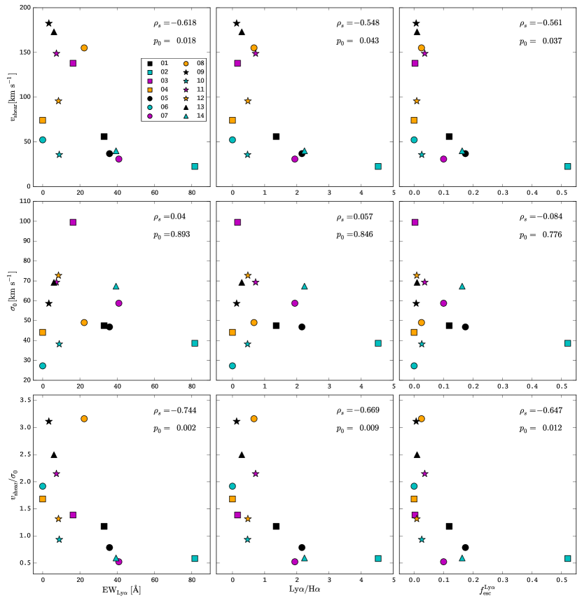
Figure 11: Relations between global Ly$\alpha$ properties of the LARS galaxies to global kinematical parameters $v_{\mathrm{shear}}$, $\sigma_{0}$ and $v_{\mathrm{shear}}/\sigma_{0}$

We now explore trends between global kinematical properties derived from the ionised gas in the LARS galaxies and their Ly$\alpha$ observables determined in Paper II, namely Ly$\alpha$ escape fraction $f_{\mathrm{esc}}^{\mathrm{Ly\alpha}}$, ratio of Ly$\alpha$ to H$\alpha$ flux $\mathrm{Ly}\alpha/\mathrm{H}\alpha$, and Ly$\alpha$ equivalent width $\mathrm{EW}_{\mathrm{Ly\alpha}}$. Fore reference, we list these quantities here again in Table10. We recall that Ly$\alpha$/H$\alpha$ is the observed flux ratio, while $f_{\mathrm{esc}}$ is determined from the intrinsic luminosities, i.e. after correcting the fluxes for dust-reddening.

Regarding the qualitative classification of the $v_{\mathrm{LOS}}$ maps in Sect. 5.1 into rotating disks, perturbed rotators and objects showing complex kinematics there is no preference in any of the globally integrated Ly$\alpha$ observables. Both the maximum and the minimum of these observables occur in complex kinematics class. Therefore, just the qualitative appearance of the velocity field seems not to predict whether the galaxy is a LAE or not.

In the previous section we showed that within the LARS sample higher SFRs are found in galaxies that have higher $\sigma_{0}$ and higher $v_{\mathrm{shear}}$ measurements and that galaxies of higher mass show also higher $v_{\mathrm{shear}}$ values and higher $v_{\mathrm{shear}}/\sigma_{0}$ ratios (Fig. 9 and Fig. 10). We now compare our $v_{\mathrm{shear}}$, $\sigma_{0}$ and $v_{\mathrm{shear}}/\sigma_{0}$-ratios to the aperture integrated Ly$\alpha$ observables $\mathrm{EW}_{\mathrm{Ly\alpha}}$, Ly$\alpha$/H$\alpha$ and $f_{\mathrm{esc}}^{\mathrm{Ly\alpha}}$ from Paper II. We do this in form of a graphical 3$\times$3 matrix in Fig. 11. In each panel we include the Spearman rank correlation coefficient $\rho_{s}$ and the likelihood $p_{0}$ to reject the null-hypothesis.

From the centre row in Fig. 11 it is obvious that none of the Ly$\alpha$ observables correlates with the averaged intrinsic velocity dispersion $\sigma_{0}$. As $\sigma_{0}$ correlates positively with SFR, this signifies that the observed Ly$\alpha$ emission is a bad star formation rate calibrator. In Fig. 11 it is also evident, that galaxies with higher shearing velocities ($v_{\mathrm{shear}}\gtrsim 50$ km s^-1) have preferentially lower $\mathrm{EW}_{\mathrm{Ly\alpha}}$, lower Ly$\alpha$/H$\alpha$ and lower $f_{\mathrm{esc}}^{\mathrm{Ly\alpha}}$. Therefore, according to the above presented $M_{\star}$-$v_{\mathrm{shear}}$ relation (Sect. 6.3.2) Ly$\alpha$ emitters are preferentially found among the systems with $M_{\star}\lesssim 10^{10}$M_⊙ in LARS. This deficiency of strong Ly$\alpha$ emitters among high mass systems was already noted in Paper II. Here we see this trend now from a kinematical perspective. Also, a low $v_{\mathrm{shear}}$ value, although a necessary condition, seems not to be sufficient to have significant amounts Ly$\alpha$ photons escaping (e.g LARS 6). Again, this shows that Ly$\alpha$ escape from galaxies is a complex multi-parametric problem.

Although the LARS sample is small, the result that 7 of 8 non-LAEs have $v_{\mathrm{shear}}/\sigma_{0}>1$ and 4 of 6 LAEs have $v_{\mathrm{shear}}/\sigma_{0}<1$ signals that dispersion-dominated kinematics are an important ingredient in Ly$\alpha$ escape. Again, lower $v_{\mathrm{shear}}/\sigma_{0}$ ratios are found in lower $M_{\star}$ objects in our sample and $\sigma_{0}$ is uncorrelated with $M_{\star}$. Therefore the correlation between Ly$\alpha$ observables and $v_{\mathrm{shear}}/\sigma_{0}$ is a consequence of the correlation between Ly$\alpha$ observables and $M_{\star}$. Nevertheless, low $v_{\mathrm{shear}}/\sigma_{0}$ ratios also state that the ionised gas in those galaxies must be in a turbulent state. High SFR appears to be connected to an increase turbulence, but it is currently not clear whether the processes that cause star formation or feedback from star formation are responsible for the increased turbulence (Sect. 6.3.1). Regardless of the causal relationship between SFR and $\sigma_{0}$, our results support that Ly$\alpha$ escape is being favoured in low-mass systems undergoing an intense star formation episode. Similarly Cowie et al. (2010) found that in a sample of UV bright $z\sim 0.3$ galaxies LAEs are primarily the young galaxies that have recently become strongly star forming. In the local Universe dispersion-dominated systems with $v_{\mathrm{shear}}/\sigma_{0}<1$ are rare, but they become much more prevalent at higher redshifts (Wisnioski et al. 2015). Coincidentally, the number density of LAEs rises towards higher redshifts (Wold et al. 2014). Therefore we speculate, that dispersion dominated kinematics are indeed a necessary requirement for a galaxy to have a significant amount of Ly$\alpha$ photons escaping.

6.5 Ly$\alpha$ extension and H$\alpha$ kinematics

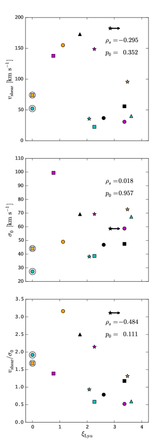
Figure 12: Relations between $\xi_{\mathrm{Ly\alpha}}$ – the relative Petrosian extension of Ly$\alpha$ as defined in Hayes et al. (2013) – and global kinematical parameters $v_{\mathrm{shear}}$, $\sigma_{0}$ and $v_{\mathrm{shear}}/\sigma_{0}$ with symbols according to the legend in Fig. 9. For galaxies with no Ly$\alpha$ emission (LARS 4 and LARS 6, circled symbols) $\xi_{\mathrm{Ly\alpha}}$ is defined as zero and for LARS 9 the measured $\xi_{\mathrm{Ly\alpha}}$ presents a lower limit (cf. Hayes et al. 2013). Spearman rank correlation coefficients $\rho_{s}$ and corresponding $p_{0}$ values are calculated excluding the LARS 4 and LARS 6.

All of the LARS LAEs show a significantly more extended Ly$\alpha$ morphology compared to their appearance in H$\alpha$ or UV continuum. These large-scale Ly$\alpha$ haloes appear to completely encompass the star-forming regions. LARS 1, LARS 2, LARS 5, LARS 7, LARS 12 and LARS 14 are the most obvious examples of extended Ly$\alpha$ emission, but the phenomenon is visible in all our objects – even for those galaxies that show Ly$\alpha$ in absorption (Fig. 5, 6 and 7; cf. Hayes et al. (2013) and Paper II). At high redshift the ubiquity of extended Ly$\alpha$ haloes around LAEs was recently revealed by Wisotzki et al. (2015) on an individual object-by-object basis. However, in contrast to the LARS Ly$\alpha$ haloes, the high-$z$ haloes appear to have $\sim$10$\times$ larger extents at a given continuum radius (Wisotzki et al. 2015, their Fig. 12). In order to quantify the spatial extent of observed relative to intrinsic Ly$\alpha$ emission we defined in Hayes et al. (2013) the Relative Petrosian Extension $\xi_{\mathrm{Ly\alpha}}$ as the ratio of the Petrosian radii at $\eta=20\%$ (Petrosian 1976) measured in Ly$\alpha$ and H$\alpha$: $\xi_{\mathrm{Ly\alpha}}=R_{\mathrm{P20}}^{\mathrm{Ly\alpha}}/R_{\mathrm{P20}}^{\mathrm{H\alpha}}$. For reference we list the $\xi_{\mathrm{Ly\alpha}}$ values of the LARS galaxies here again in Table 10. Based on an anti-correlation between $\xi_{\mathrm{Ly\alpha}}$ and UV slope we conjectured that smaller Ly$\alpha$ haloes occur in galaxies that have converted more of their circum-galactic neutral gas into forming stars and subsequently dust (Hayes et al. 2013). In such a scenario the larger extent of high-$z$ Ly$\alpha$ haloes could be related to the circum-galactic gas-reservoirs being larger in the early universe.

In Fig. 12 we show that there are no significant correlations between $\xi_{\mathrm{Ly\alpha}}$ and the global kinematical H$\alpha$ parameters $v_{\mathrm{shear}}$, $\sigma_{0}$ and $v_{\mathrm{shear}}/\sigma_{0}$. Therefore we reason that the kinematics of the interstellar medium do not strongly influence the appearance of the haloes and that the Ly$\alpha$ halo phenomenon is only related to the presence of a full gas-reservoir. Further 21cm HI imaging of the LARS galaxies at high spatial resolution is needed to test this scenario.

7 Summary and conclusions

We obtained the following results From our integral field spectroscopic observations of the H$\alpha$ line in the LARS galaxies:

1. Half of the LARS galaxies show complex H$\alpha$ kinematics. Only two galaxies have kinematical properties consistent with a rotating disk and in five a disturbed rotational signature is apparent. With respect to Ly$\alpha$ escape we find no preference of high EW_Lyα or high $f_{\mathrm{esc.}}^{\mathrm{Ly\alpha}}$ values towards any of those classes but the minimum and maximum values occur both in objects showing complex kinematics in our sample.

2. A common feature in all LARS galaxies are high H$\alpha$ velocity dispersions. With $v_{\mathrm{FWHM}}\gtrsim 100$ km s^-1 our measurements are in contrast to values typically seen in local spirals, but in high-$z$ star-forming galaxies such high values appear to be the norm.

3. While we could not infer a direct relation between spatially resolved kinematics of the ionised gas and photometric Ly$\alpha$ properties for all LARS galaxies, in individual cases our maps appear qualitatively consistent with outflow scenarios that promote Ly$\alpha$ escape from high-density regions.

4. Currently a spatially resolved comparison of our H ii velocity fields to our H i data is severely limited, since the scales resolved by the radio observations are significantly larger. However, for one galaxy (LARS 7) the difference between globally integrated velocity dispersion of ionised and neutral gas offers a viable explanation for the escape of significant amounts of Ly$\alpha$ photons.

5. From our H$\alpha$ velocity maps we derive the non-parametric statistics $v_{\mathrm{shear}}$, $\sigma_{0}$ and $v_{\mathrm{shear}}/\sigma_{0}$ to quantify the kinematics of the LARS galaxies globally. Our $v_{\mathrm{shear}}$ values range from 30 km s^-1 to 180 km s^-1 and our $\sigma_{0}$ values range from 40 km s^-1 to 100 km s^-1. For our ratios $v_{\mathrm{shear}}/\sigma_{0}$ we find a median of 1.4 and five of the LARS galaxies are dispersion-dominated systems with $v_{\mathrm{shear}}/\sigma_{0}<1$.

6. Fully consistent with other IFS studies $\sigma_{0}$ is positively correlated with star formation rate in the LARS galaxies. We also find strong correlations between $M_{\star}$ and $v_{\mathrm{shear}}$, $M_{\star}$ and $v_{\mathrm{shear}}/\sigma_{0}$, and SFR and $v_{\mathrm{shear}}$. In view of the $M_{\star}$-$v_{\mathrm{shear}}$ the SFR- $v_{\mathrm{shear}}$ correlation implies that more massive galaxies have higher overall star formation rates in our sample.

7. The Ly$\alpha$ properties EW_Lyα, Ly$\alpha$/H$\alpha$ and $f_{\mathrm{esc.}}^{\mathrm{Ly\alpha}}$ do not correlate with $\sigma_{0}$, but they correlate with $v_{\mathrm{shear}}$ and $v_{\mathrm{shear}}/\sigma_{0}$ (Fig. 11). We find no correlation between the global kinematical statistics and the extent of the Ly$\alpha$ halo.

8. 4 of 6 LARS LAEs are dispersion-dominated systems with $v_{\mathrm{shear}}/\sigma_{0}<1$ and 7 of 8 non-LAEs have $v_{\mathrm{shear}}/\sigma_{0}>1$.

Observational studies of Ly$\alpha$ emission in local-universe galaxies have so far focused on imaging and UV spectroscopy (for a recent review see Hayes 2015). Here we provided for the first time empirical results from IFS observations for a sample of galaxies with known Ly$\alpha$ observables. In our pioneering study we focused on the spectral and spatial properties of the intrinsic Ly$\alpha$ radiation field as traced by H$\alpha$. We found a direct relation between the global non-parametric kinematical statistics of the ionised gas and the Ly$\alpha$ observables $f_{\mathrm{esc.}}^{\mathrm{Ly\alpha}}$ and $\mathrm{EW}_{\mathrm{Ly\alpha}}$, and our main result is that dispersion dominated systems favour Ly$\alpha$ escape. The prevalence of LAEs among dispersion dominated galaxies could be simply a consequence of these systems being the lower mass systems in our sample – a result already found in Paper II. However, the observed turbulence in actively star-forming systems should be related to ISM conditions that ease Ly$\alpha$ radiative transfer out of high density environments. In particular, if turbulence is a direct consequence of star formation, then the energetic input from the star formation episode might also be powerful enough to drive cavities through the neutral medium into the lower density circum-galactic environments. Of course, the kinematics of the ionised gas offer only a limited view of the processes at play and in future studies we attempt to connect our kinematic measurements to spatial mappings of the ISMs ionisation state. The synergy between IFS data, space based UV imaging and high resolution H i observations of nearby star forming galaxies will be vital to build a coherent observational picture of Ly$\alpha$ radiative transport in galaxies.

Appendix A Notes on individual objects

In the following we detail the observed H$\alpha$ velocity fields for each galaxy. We compare our maps to the photometric Ly$\alpha$ properties derived from the HST images from Paper II and H i observations from Paper III (see Sect. 4).

A.1 LARS 1 (Mrk 259)

With $L_{\mathrm{Ly\alpha}}=8\times 10^{41}$ erg s^-1 and $\mathrm{EW}_{\mathrm{Ly\alpha}}=33$ Å LARS 1 is a strong Ly$\alpha$ emitting galaxy. A detailed description of the photometric properties of this galaxy was presented in Paper I. If LARS 1 would be at high-$z$, it would easily be selected in conventional narrow-band imaging surveys (Paper IV). The galaxy shows a highly irregular morphology. Its main feature is UV-bright complex in the north-east that harbours the youngest stellar population. As noted already in Paper II filamentary structure emanating from the north-eastern knot is seen in H$\alpha$. Towards the south-east numerous smaller star-forming complexes are found that blend in with an older stellar population.

Contrasting the irregular appearance, the line of sight velocity field of LARS 1 is rather symmetric. The velocity field is consistent with a rotating galaxy. The kinematical centre is close to centre of the PMAS FoV and the kinematical axis appears to run from the north-west to the south-east. We measure $v_{\mathrm{shear}}=56\pm 1$ km s^-1. The GBT single dish H i spectrum of this source is reminiscent of a classic double-horn profile, also an obvious sign of rotation, with a peak separation consistent with our $v_{\mathrm{shear}}$ measurement.

The highest velocity dispersions ($v_{\mathrm{FWHM}}\approx 150$ km s^-1) are found in the north-eastern region. Here LARS 1 also shines strong in Ly$\alpha$. But while a fraction of Ly$\alpha$ appears to escape directly towards us, a more extended Ly$\alpha$ halo around this part is indicative of resonant scatterings in the circum-galactic gas (cf. also Östlin et al. 2014). Contrary, in the south-western part of the galaxy, where we observe the lowest velocity dispersions ($v_{\mathrm{FWHM}}\approx 70$ km s^-1), Ly$\alpha$ photons do not escape along the line of sight.

A.2 LARS 2 (Shoc 240)

Everywhere in LARS 2 where H$\alpha$ photons are produced, Ly$\alpha$ photons emerge along the line of sight. LARS 2 is the galaxy with the highest global escape fraction of Ly$\alpha$ photons ($f^{\mathrm{Ly}\alpha}_{\mathrm{esc.}}=52.1$%) and the highest Ly$\alpha$/H$\alpha$ ratio (Ly$\alpha$/H$\alpha=4.53$).

With $v_{\mathrm{shear}}=23\pm 2$ km s^-1, LARS 2 shows the smallest $v_{\mathrm{shear}}$ in our sample. However, we consider this value as a lower limit since we missed in our pointing the southernmost star forming knot. Our observed velocity field appears to be disturbed, but we could envision a kinematical axis orthogonal to the photometric major axis - i.e. roughly from west to east. This idea is supported by our VLA imaging of this source (see Fig. 7 in Paper III, ). The H i velocity field also indicates $v_{\mathrm{shear}}\approx 30$ km s^-1, meaning that our incomplete measurement gives a sensible lower limit. Within the observed region our velocity dispersion map is rather uniform, with $v_{\mathrm{VFWHM}}\approx 100$ km s^-1.

A.3 LARS 3 (Arp 238)

LARS 3 is the south-eastern nucleus of the violently interacting pair of similar sized spiral galaxies Arp 238. With a global $f_{\mathrm{esc}}^{\mathrm{Ly\alpha}}=0.1$ and $L_{\mathrm{Ly\alpha}}=10^{41}$erg s^-1 this dust rich luminous infrared galaxy is a relatively weak Ly$\alpha$ emitter. VLA H i imaging reveals an extended tail towards the west. This tidal tail is much larger than the optical dimensions of the pair Arp 238 (see also Cannon et al. 2004, for similar extended tidal H i structures around the Ly$\alpha$ emitting star bursts Tol 1924-416 and IRAS 08339+6517).

In H$\alpha$ the main kinematical axis runs from west to east and the radial velocity field appears symmetric, although slightly disturbed towards the north and the south. We measure $v_{\mathrm{shear}}\approx 140$ km s^-1, a value which is in the domain of typical maximum velocities of inclination corrected H$\alpha$ rotation curves of spiral galaxies (e.g. Epinat et al. 2008a, 2010; Erroz-Ferrer et al. 2015). With $v_{\mathrm{FWHM}}\gtrsim 300$ km s^-1 highest velocity dispersions are observed in the western part. The largest Ly$\alpha$ surface brightness is also observed in the western part of the nucleus. Ly$\alpha$ appears in absorption in the eastern region, where we also see a minimum in velocity dispersions with $v_{\mathrm{FWHM}}\approx 70$ km s^-1.

A.4 LARS 4 (SDSS J130728.45+542652.3)

Although LARS 4 is similar to LARS 1 in terms of dust content and star formation rate, globally this galaxy shows Ly$\alpha$ in absorption. The galaxy can be photometrically decomposed into two main components: an elongated lower surface brightness structure in the west and a more puffed up and luminous companion in the east. The eastern structure is tilted at $\approx 40^{\circ}$ with respect to the western one.

Compared to the highly irregular morphology in UV and H$\alpha$, the radial velocity field appears rather regular, with a moderate amplitude of $v_{\mathrm{shear}}\approx 75$ km s^-1 along a well defined axis from west to east. The kinematic centre appears to be right between the two photometric components, indicating that the observed shearing is the velocity difference between the merging components and not a consequence of rotation. The lack of a well defined simple and organised disk is further supported by the absence of a double-horn profile in the GBT single-dish H i profile. Nevertheless, higher sensitivity VLA imaging results show a coherent velocity field on larger scales with an amplitude comparable to $v_{\mathrm{shear}}$ ( Paper III, their Fig. 9).

In the dispersion map, the two components are clearly distinguishable, with the eastern component showing higher velocity dispersions ($v_{\mathrm{FWHM}}\approx 100$ km s^-1) than the western ($v_{\mathrm{FWHM}}\approx 65$ km s^-1). In both regions, however, Ly$\alpha$ is seen in absorption. The highest velocity dispersions are observed at the boundary region where the two components are separated photometrically - but also here only little Ly$\alpha$ is escaping.

A.5 LARS 5 (Mrk 1486)

In the HST images LARS 5 appears as a small (i.e. projected diameter $d\approx 5$ kpc) highly inclined edge-on disk. Within the apparent disk Ly$\alpha$ appears in absorption but the galaxy shows an extended halo, which is azimuthally symmetric at low surface brightness isophotes, while brighter isophotes resemble more the elongated H$\alpha$ shape. Most prominent in the H$\alpha$ image are filamentary “fingers” extending below and above the disk, reminiscent of an outflowing wind.

Although the profile of our single-dish H i observations shows multiple peaks close to the noise level that might correspond to the peaks of a faint double horn profile (Paper III), our H$\alpha$ kinematics appear incompatible with a typical disk scenario: Firstly, our measured $v_{\mathrm{shear}}=37$ km s^-1 indicates a very low rotation curve amplitude - untypical even for a small disk (e.g. in the largest H$\alpha$ disk sample of Epinat et al. 2010, for $d\leq 5$ kpc the maximum rotation curve velocity is on average 95 km s^-1). Secondly, there is apparent asymmetry in the spatial distribution of the $v_{\mathrm{LOS}}$ values, i.e. a large sector in the south-west characterised by similar line of sight velocities ($v_{\mathrm{LOS}}\sim+20$ km s^-1), while only a small sector in the north-east shows blue-shifted H$\alpha$ emission ($v_{\mathrm{LOS}}\sim-40$ km s^-1).

The most prominent feature in the velocity dispersion map is a biconical zone of increasing velocity dispersions (from $\sim$120 km s^-1 to $\sim$220 km s^-1) with increasing distance from the centre. The base of this zone coincides the brightest region in UV and H$\alpha$ in the south-western sector. We note that the seeing PSF FWHM for this observation is 1.3″, thus $\sim$2$\times$ the extend of the 0.5″$\times$0.5″ spaxels used on LARS 5. However, as the kinematical centre is not co-spatial with the base of the cones, and since the velocity gradient around the base of the cone is very weak we are confident that this feature is real and not caused by PSF smearing effects.

A.6 LARS 6 (KISSR 2019)

With $\lesssim 1$ M_⊙yr^-1 conversion of gas into stars LARS 6 shows the lowest star formation rate in the sample (Hayes et al. 2014). The main star forming knot is in the north with a tail of much smaller and less luminous knots extending to the south. In our seeing limited data cubes we can not disentangle these individual knots photometrically. Ly$\alpha$ is seen in absorption, even on the smallest scales.

Shearing is observed between the main component and the tail, although the amplitude is moderate ($v_{\mathrm{shear}}=52$ km s^-1). The main component also shows higher velocity dispersions ($v_{\mathrm{VFWHM}}\approx 70$ km s^-1) than the tail ($v_{\mathrm{VFWHM}}\approx 50$ km s^-1). Overall this galaxy has the lowest observed velocity dispersion in the sample.

Our GBT single-dish H i measurements are severely contaminated by the nearby field spiral UGC 10028. However, newly obtained but as of yet unpublished VLA D-configuration images allow a first-order separation from LARS 6 and this companion. From these data, coherent rotation is present in the H i gas associated with LARS 6 at a level roughly consistent with the $v_{\mathrm{shear}}$ estimate we obtain from PMAS.

A.7 LARS 7 (IRAS F13136+2938 )

In the continuum LARS 7 resembles a highly inclined disk comparable to LARS 5. But, in H$\alpha$ an almost azimuthally symmetric structure emerges that is highly distended with respect to the elongated continuum morphology. Moreover, two extended low surface brightness red lobes are found at the opposite ends of the inclined disk, reminiscent of a shell like structure. This is suggestive of a recent merger event (e.g. Bettoni et al. 2011). In Ly$\alpha$ images LARS 7 appears even more extended, with the bright isophotes following the H$\alpha$ shape and low-surface brightness isophotes resembling a more scaled up version of the apparent disk.

For similar reasons as outlined for LARS 5 in Sect. A.5, our H$\alpha$ kinematics argue against a typical disk scenario: We observe a low shearing amplitude; with $v_{\mathrm{shear}}=31$ km s^-1 even lower than in LARS 5. Moreover, the line of sight velocity maps appears disturbed compared to that expected for a classical disk. Our GBT single dish H i observations reveal a single broad ($92$ km s^-1) line. LARS 7 is the only object where the GBT line-width is incompatible to its integrated H$\alpha$ linewidth (cf. Sect. 6.2). A main kinematical axis can be envisioned to run from north east to south west along the continuum major axis. But in the north west and south east the $v_{\mathrm{LOS}}$ values do not follow this weak gradient at all. Overall the galaxy shows high velocity dispersion in H$\alpha$ ($v_{\mathrm{FWHM}}\gtrsim 160$ km s^-1), with the lowest values occurring in north east ($v_{\mathrm{FWHM}}\approx 120$ km s^-1), where the brightest fluxes in Ly$\alpha$ and the highest Ly$\alpha$/H$\alpha$ ratios are observed.

A.8 LARS 8 (SDSS-J125013.50+073441.5)

LARS 8 appears a face-on disk with the highest metalicity of the sample. The apparent disk also possesses a highly dust obscured nucleus. Nevertheless, there is a high degree of irregularity compared to classical disks and spiral arms are not well defined. As traces of shell-like structures are visible in the inner parts and in the outskirts of the galaxy (cf. Fig. 6 in Paper I), LARS 8 can be classified as a shell system hinting at a recent merger event (Bettoni et al. 2011, e.g.). The Ly$\alpha$ light distribution of LARS 8 does not resemble that seen in H$\alpha$. The brightest Ly$\alpha$ zone is in the north of the disk, while in the south Ly$\alpha$ appears only in absorption. At lower surface brightness isophotes a Ly$\alpha$ halo becomes visible. With an equivalent width $\mathrm{EW}_{\mathrm{Ly\alpha}}=20.3$Å this galaxy would be selected as LAE in conventional narrow-band surveys.

Our $v_{\mathrm{LOS}}$ map seems disk like. Assuming an infinitely thin disk the ellipticity of 0.2 (Guaita et al. 2015) implies an inclination of 40^∘, hence our observed $v_{\mathrm{shear}}=155$ km s^-1 translates to $v_{\mathrm{max}}=241$ km s^-1. The GBT single-dish H i profile shows a broad, possibly double peaked profile. Although these peaks are not significantly separated from the overall H i signal, the implied velocity difference of $\sim$300 km s^-1 appears consistent with our $v_{\mathrm{shear}}$ measurement. The orientation of the velocity field from VLA interferometric H i observations is qualitatively consistent with our PMAS H$\alpha$ observations, although at the VLA D-configuration beam size of 72″ LARS 8 appears only marginally resolved.

Elevated velocity dispersions with $v_{\mathrm{FWHM}}\gtrsim 160$ km s^-1 are apparent to extend orthogonal to the kinematical axis along the 0  km s^-1 iso velocity contour. In the other parts of the $v_{\mathrm{FWHM}}$ map is rather flat, typically with $v_{\mathrm{FWHM}}\sim 100$ km s^-1 - a value that is also still commonly observed within the sample of 153 local spirals by Epinat et al. (2010). Given the strong gradient in the velocity field, the observed elevated velocity dispersions are likely a result of PSF smearing effects.

A.9 LARS 9 (IRAS 08208+2816 )

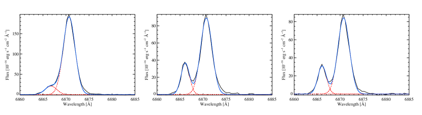
Figure 13: Representative LARS 9 H$\alpha$ line profiles in blue hatched region of Fig. 6 described by a fit using two Gaussian components. The red dashed lines show the individual components and the blue line shows the sum, while the black line shows the profile as observed. For all profiles shown the single component fit used to create the map shown in Fig. 6 converged on the stronger red component.

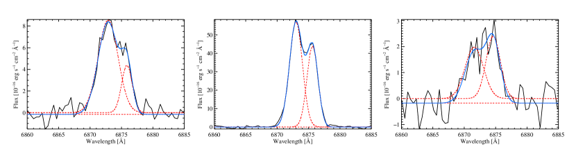
Figure 14: Representative LARS 9 H$\alpha$ line profiles in red hatched region of Fig. 6, similar to Fig. 13. The single component fit used to create the map shown in Fig. 6 converged on the stronger blue component in the centre panel, but for the profiles shown in the left and right panel the single component fit is artificially broadened.

This luminous infrared galaxy has highly irregular morphology. Numerous star forming knots are visible in H$\alpha$ along two arms of large extend that are connected to central, very bright H$\alpha$ nucleus. We note that at the end of the southern-tail a foreground star appears in projection; contributions from this star have been masked out in the PMAS data. In LARS 9 Ly$\alpha$ is almost everywhere absorbed along the line of sight towards the star forming regions. Nevertheless, this galaxy is embedded in a faint extended Ly$\alpha$. Morphologically, this fuzz broadly traces a scaled up version of its optical and H$\alpha$ shape. Having a globally integrated Ly$\alpha$ luminosity of $L_{\mathrm{Ly\alpha}}\approx 3\times 10^{41}$ erg s^-1 and an equivalent width of $EW_{\mathrm{Ly\alpha}}\approx 8$Å, this galaxy would not be selected by its Ly$\alpha$ emission at high-$z$ in conventional narrow-band surveys.

Since LARS 9 extends more than $\sim 0.5$′ on the sky, we needed to cover it with two PMAS 16″$\times$16″ pointings (Fig. 6). The line of sight velocity field for this galaxy is very peculiar. From the north to the centre a weak ($\sim 100$ km s^-1) gradient from blue-shifted to systemic velocity is apparent. From the centre this weak gradient continues towards the south. The southern tail then shows an opposite gradient from red- to blue-shifts. We note that in this south- and south-western zone a single Gaussian often is not an optimal representation of the observed H$\alpha$ lines. In this zone the spectral profile is sometimes asymmetric with an extended red or blue wing, but often it shows also clearly double peaked morphology (for examples see Fig. 13). In some these regions our fit tries to capture both lines, hence the obtained line of sight velocity is centred between the peaks and the linewidth appears very broad (e.g. left and right panel of Fig. 14). In some other spaxels, when the secondary peak is very weak or when only an extended wing is seen, the fit converges to the stronger line. The affected zones have hatched rectangles overlaid in Fig. 6. These zones harbour a kinematical distinct secondary component. This secondary component does not follow the large scale motions of the northern component, to which also the nucleus belongs. We indicate by red- and blue-hatchings in Fig. 6 the regions of this component that are red- and blue-shifted with respect to the systemic velocity (as given by the nucleus). As a natural outcome from this qualitative analysis the emission in south-eastern tail of LARS 9 is solely coming from this secondary component. We note that also only at the end of this tail a significant fraction of Ly$\alpha$ photons appear to escape towards the observer.

From our PMAS observation we conclude that LARS 9 is a closely interacting pair of galaxies in an advanced stage of merging. The interaction scenario is also supported by our 21cm observations. The integrated GBT spectrum shows a broad single line, indicating that the bulk of the H i is not partaking in an ordered flat rotation. LARS 9 was only marginally resolved in our VLA H i maps (Paper III). However, as of yet unpublished VLA C configuration observations (K. Fitzgibbon, in prep.) show extended H i towards the west, enclosing the galaxy SDSS J082353.65+280622.2. For this galaxy no spectroscopic redshift is available, but the photometric redshift agrees with being associated to LARS 9. These observations therefore strongly suggests that a third system is significantly involved in the interaction. Moreover, the VLA C-configuration observations of LARS 9 show a peak in the second-moment maps that trace the random motions of H i that coincides spatially with the zones of multiple H ii components in our PMAS maps . Hence, at these locations (hatched regions in Fig. 6) Ly$\alpha$ photons of both distinct kinematical components are likely scattered by H i at resonance.

A.10 LARS 10 (Mrk 0061)

Similar to LARS 1 this galaxy appears morphologically to be in an advanced merger state. It possesses a large UV bright core in the north-west and a spur of smaller, less luminous star forming regions towards the south-east. Several redder low-surface brightness structures are seen outside the main body of the galaxy, reminiscent of the appearance of shell galaxies (e.g. Marino et al. 2009; Bettoni et al. 2011). From the central star-forming parts Ly$\alpha$ is only seen in absorption, while at larger radii a faint halo emerges. When considering solely the central parts the galaxy would remain undetected in high-$z$ LAE surveys since $\mathrm{EW_{\mathrm{Ly\alpha}}}=8$Å. But, when integrating over the lower-surface brightness emission $\mathrm{EW_{\mathrm{Ly\alpha}}}$ rises to 31Å and with its luminosity of $L_{\mathrm{Ly\alpha}}=2\times 10^{41}$erg s^-1 it would be within the sensitivity of the deepest contemporary LAE surveys (Rauch et al. 2008; Bacon et al. 2015).

The line of sight velocity field is symmetric and consistent with rotation and contrasts the irregular continuum morphology. The velocity gradient running from the south-east to the north-west is weak and we measure $v_{\mathrm{shear}}=36$ km s^-1. The seeing for this observation was quite substantial (1.5″ FWHM, i.e 3$\times$ the size of the $0.5$″$\times$0.5″ spaxels). Despite the weak gradient, this leads to non-negligible PSF smearing effects in the dispersion map. Moreover, due to the short exposure time and the rather low H$\alpha$ flux this galaxy has the lowest SNR per spaxel of the whole sample; this manifests in a noisy $v_{\mathrm{FWHM}}$ map. Both of these effects make essentially local disturbances in the velocity dispersion untraceable in our LARS 10 dataset, but our flux weighted global measurement of $\sigma_{0}\approx 40$ km s^-1 is robust against these nuisances.

The GBT integrated H i spectrum shows a broad single line profile ($\sim$280 km s^-1 FWHM), however at low signal to noise. This appears hard to reconcile with the H$\alpha$ results. If real, it might indicate that a large fraction of neutral gas in and around LARS 10 is kinematically in a different state than the gas around the galaxy’s star forming regions.

A.11 LARS 11 (SDSS J140347.22+062812.1)

This galaxy appears as a highly inclined edge-on disk in the continuum and UV that is slightly thicker when seen in H$\alpha$. According to the H$\alpha$ and UV emission, stronger star formation occurs in the south-eastern zone of the projected disk. In Ly$\alpha$ a mildly extended halo above and below the plane is visible, with the isophotal contours approximately preserving the axis ratio of H$\alpha$. Within the disk Ly$\alpha$ occurs exclusively in absorption.

Running along the disk from the north-west to the south-east a strong gradient in the $v_{\mathrm{LOS}}$ map is apparent. The observed shearing amplitude $v_{\mathrm{shear}}=150$ km s^-1 is consistent with this gradient being caused by rotation (e.g. Epinat et al. 2008a, 2010; Erroz-Ferrer et al. 2015). Unfortunately the beam of our GBT single-dish H i observations is likely contaminated by other sources. Nevertheless, within the multiple peaks in the GBT spectrum a double-horn profile at a velocity separation consistent with our H$\alpha$ $v_{\mathrm{shear}}$ measurement is visible. Although the projected height of the disk is similar to the PSF FWHM, the dispersion map shows traces of higher velocity dispersions above and below the disk ($v_{\mathrm{VFWHM}}\approx 200$ km s^-1) than within ($v_{\mathrm{VFWHM}}\approx 150$ km s^-1), especially around the star-forming regions in the south east. We note, however, that the elevated dispersions near the kinematic centre are caused by PSF smearing of the strong gradient in the $v_{\mathrm{LOS}}$ field.

A.12 LARS 12 (LEDA 27453)

Because of its modest $\mathrm{EW}_{\mathrm{Ly\alpha}}=13$Å this UV bright merger would not be selected as a LAE at high-$z$. At its brightest knot in UV and H$\alpha$ the galaxy shows Ly$\alpha$ only in absorption. Only at larger radii, where a number of fainter star forming regions can be appreciated, Ly$\alpha$ appears in emission. Moreover, LARS 12 is embedded in a faint, low surface brightness Ly$\alpha$ halo.

The non-regular H$\alpha$ velocity field indicates complex kinematics. In the north-western corner a strong $\sim 140$ km s^-1 gradient over $\sim 1.5$″ ($\sim 2.8$ kpc at $d_{\mathrm{LARS12}}=470.5$ Mpc) is observed, but from there towards the south-west the velocity field is essentially flat. The high velocity and velocity dispersion in the values seen in the south are not significant, as the low SNR of this broad line in these binned spaxels lead to a 50% error on the determined $v_{\mathrm{LOS}}$ and $\sigma_{0}$ value. We note that because of PSF smearing effects the strong velocity gradient is responsible for the region of elevated velocity dispersions in the north-western corner.

For LARS 12 adaptive optics Paschen $\alpha$ IFS observations have been presented in Gonçalves et al. (2010) - Object ScUVLG 093813 in their nomenclature. Their line-of-sight velocity field is qualitatively fully consistent with ours, but their higher resolution data allows to pinpoint the highest redshifted values directly to the two filaments that extent towards the north-west. Since they are not affected by PSF smearing their dispersion map is not contaminated by high-velocity dispersions in the north-west. Of course, our artifact in the south is also absent from their map. Nevertheless, their $\sigma_{0}$ value of 62 km s^-1 is in good agreement with our measurement of 72 km s^-1.

A.13 LARS 13 (IRAS 01477+1254)

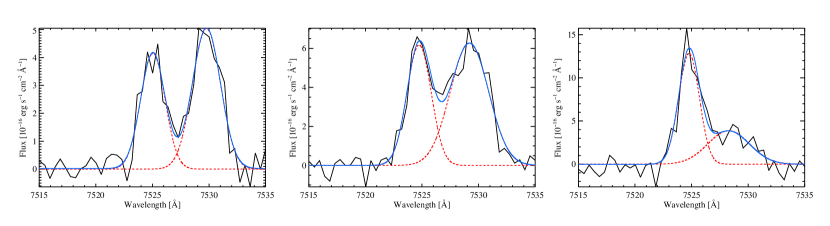
Figure 15: Representative LARS 13 H$\alpha$ line profiles in blue hatched region of Fig. 7, similar to Fig. 13. The single component fit used to create the map shown in Fig. 7 converged on the stronger blue component in the right panel, but for the profiles shown in the left and canter panel the single component fit is artificially broadened.

Based on its highly irregular morphology this starburst system is clearly interacting. As LARS 13 shows a narrow Ly$\alpha$ equivalent width ($\mathrm{EW}_{\mathrm{Ly\alpha}}=6$ Å), it would not be selected as a LAE at high redshift in conventional narrow-band surveys. Overall only 1% of Ly$\alpha$ photons are escaping and the resulting Ly$\alpha$ luminosity is $L_{\mathrm{Ly\alpha}}=7\times 10^{41}$ erg s^-1.

The complex $v_{\mathrm{LOS}}$ map of this galaxy is characterised by a gradient from blue- to redshifts along the east-western axis for the northern component, as well as an gradient from blue-to-redshifts from south to north for the eastern component. In the north-western zone where the longitudinally aligned structure overlaps with the latitudinally aligned one, our single component Gaussian is not an optimal representation of the observed H$\alpha$ line profiles. In this region the profile is often asymmetric with an extended blue wing (e.g. right panel of Fig. 15). Some spaxels show a double peaked H$\alpha$ profile (e.g. left and centre panel of Fig. 15). The affected zone has a hatched rectangle overlaid in Fig. 7. In the region where two equally strong peaks are prominent in the spectrum, our fit tries to fit a broad line that encloses both lines; these spaxels can be seen in the east running as a diagonal line of broad velocity dispersions from north-west to south-east. Spaxels east from this demarcation show an extended blue wing. We interpret this as that we are seeing separate components of ionised gas kinematics, where one component belongs to the latitudinal elongated structure while the other belongs to the longitudinal elongated one. The spatial and spectral proximity of both regions indicates that the galaxy is still in an ongoing interaction with both progenitors not having fully coalesced.

For LARS 13 adaptive optics Paschen $\alpha$ IFS observations have been presented in Gonçalves et al. (2010) - object ScUVLG 015028 in their nomenclature. However, their small FoV allows them only to sample emission from the strongest star forming region in the western part, so they do not have any information on the longitudinally aligned eastern part. Consequently, their observed $v_{\mathrm{shear}}=78$ km s^-1 is lower than our value ($v_{\mathrm{shear}}=173$ km s^-1), since the north-eastern zone with highest $v_{\mathrm{LOS}}$ values in our map is not present in their data. In the zone where they have signal, there is good qualitative and quantitative agreement between our maps and their maps. In particular, they found high velocity dispersions $v_{\mathrm{FWHM}}\gtrsim 200$ km s^-1 and a weak velocity gradient in the north-western star-forming knot. We note that in this region of high velocity dispersions Ly$\alpha$ appears to escape directly towards the observer.

A.14 LARS 14 (SDSS J092600.41+442736.1)

LARS 14 is the most luminous LAE in the sample ($L_{\mathrm{Ly\alpha}}=4.2\times 10^{42}$erg s^-1). It is also classified as a green pea galaxy (Cardamone et al. 2009, see also their Fig. 7). Green pea galaxies show commonly strong Ly$\alpha$ emission and are also thought to be Lyman continuum leaking galaxies (Jaskot & Oey 2014; Henry et al. 2015; Yang et al. 2015). Visible in the HST images is a small companion in the south and tidal tails extending to the east and south (Cardamone et al. 2009). Our seeing limited data does not provide enough resolution to disentangle this structure photometrically from the main component within the datacube. Kinematically, however, we observe that the southern region shears at $\approx 60-70$ km s^-1 with respect to the northern, with not much velocity substructure seen. In the main part we observe high velocity dispersions with $v_{\mathrm{FWHM}}\approx 175$ km s^-1, dropping to $80-90$ km s^-1 towards the companion. Our modelling of the H$\alpha$ profile with a simple 1D Gaussian did not capture the extended broad wings seen in the H$\alpha$ profiles. These broad wings likely trace outflowing ionised gas, and are a feature regularly observed in pea galaxies (Yang et al. 2015).

For this galaxy adaptive optics Paschen $\alpha$ IFS observation have been presented in Gonçalves et al. (2010) and Basu-Zych et al. (2009) (object ScUVLG 92600 in their nomenclature). They report slightly higher values, both for the shear and the dispersion. Nevertheless, our derived $v_{\mathrm{shear}}/\sigma_{0}=0.6\pm 0.1$ is consistent with their value of 0.51. This ratio would be lowered by about a factor of two, if only the northern main component is considered, since its velocity offset relative to the companion dominates the shear. Noteworthy, the main component as such therefore presents the structure with the lowest $v_{\mathrm{shear}}/\sigma_{0}$ of our whole sample.

References

- Adams et al. (2011) Adams, J. J., Blanc, G. A., Hill, G. J., et al. 2011, ApJS, 192, 5
- Ahn et al. (2003) Ahn, S.-H., Lee, H.-W., & Lee, H. M. 2003, MNRAS, 340, 863
- Alonso-Herrero et al. (2009) Alonso-Herrero, A., García-Marín, M., Monreal-Ibero, A., et al. 2009, A&A, 506, 1541
- Astropy Collaboration et al. (2013) Astropy Collaboration, Robitaille, T. P., Tollerud, E. J., et al. 2013, A&A, 558, A33
- Bacon et al. (2015) Bacon, R., Brinchmann, J., Richard, J., et al. 2015, A&A, 575, A75
- Bacon et al. (2014) Bacon, R., Vernet, J., Borisiva, E., et al. 2014, The Messenger, 157, 13
- Barnes et al. (2011) Barnes, L. A., Haehnelt, M. G., Tescari, E., & Viel, M. 2011, MNRAS, 416, 1723
- Bassett et al. (2014) Bassett, R., Glazebrook, K., Fisher, D. B., et al. 2014, MNRAS, 442, 3206
- Basu-Zych et al. (2009) Basu-Zych, A. R., Gonçalves, T. S., Overzier, R., et al. 2009, ApJ, 699, L118
- Behrens & Braun (2014) Behrens, C. & Braun, H. 2014, A&A, 572, A74
- Behrens et al. (2014) Behrens, C., Dijkstra, M., & Niemeyer, J. C. 2014, A&A, 563, A77
- Bettoni et al. (2011) Bettoni, D., Galletta, G., Rampazzo, R., et al. 2011, A&A, 534, A24
- Bik et al. (2015) Bik, A., Östlin, G., Hayes, M., et al. 2015, A&A, 576, L13
- Calabretta & Greisen (2002) Calabretta, M. R. & Greisen, E. W. 2002, A&A, 395, 1077
- Cannon et al. (2004) Cannon, J. M., Skillman, E. D., Kunth, D., et al. 2004, ApJ, 608, 768
- Cappellari & Copin (2003) Cappellari, M. & Copin, Y. 2003, MNRAS, 342, 345
- Cardamone et al. (2009) Cardamone, C., Schawinski, K., Sarzi, M., et al. 2009, MNRAS, 399, 1191
- Cassata et al. (2011) Cassata, P., Le Fèvre, O., Garilli, B., et al. 2011, A&A, 525, A143
- Cassata et al. (2015) Cassata, P., Tasca, L. A. M., Le Fèvre, O., et al. 2015, A&A, 573, A24
- Chonis et al. (2013) Chonis, T. S., Blanc, G. A., Hill, G. J., et al. 2013, ApJ, 775, 99
- Christensen et al. (2012) Christensen, L., Laursen, P., Richard, J., et al. 2012, MNRAS, 427, 1973
- Ciardullo et al. (2012) Ciardullo, R., Gronwall, C., Wolf, C., et al. 2012, ApJ, 744, 110
- Cooper et al. (2008) Cooper, J. L., Bicknell, G. V., Sutherland, R. S., & Bland-Hawthorn, J. 2008, ApJ, 674, 157
- Cowie et al. (2010) Cowie, L. L., Barger, A. J., & Hu, E. M. 2010, ApJ, 711, 928
- Cox (2000) Cox, A. N. 2000, Allen’s astrophysical quantities
- Davies et al. (2011) Davies, R., Förster Schreiber, N. M., Cresci, G., et al. 2011, ApJ, 741, 69
- Diehl & Statler (2006) Diehl, S. & Statler, T. S. 2006, MNRAS, 368, 497
- Dijkstra (2014) Dijkstra, M. 2014, PASA, 31, 40
- Dijkstra et al. (2006) Dijkstra, M., Haiman, Z., & Spaans, M. 2006, ApJ, 649, 14
- Duval et al. (2014) Duval, F., Schaerer, D., Östlin, G., & Laursen, P. 2014, A&A, 562, A52
- Epinat et al. (2010) Epinat, B., Amram, P., Balkowski, C., & Marcelin, M. 2010, MNRAS, 401, 2113
- Epinat et al. (2008a) Epinat, B., Amram, P., & Marcelin, M. 2008a, MNRAS, 390, 466
- Epinat et al. (2008b) Epinat, B., Amram, P., Marcelin, M., et al. 2008b, MNRAS, 388, 500
- Erb et al. (2014) Erb, D. K., Steidel, C. C., Trainor, R. F., et al. 2014, ApJ, 795, 33
- Erroz-Ferrer et al. (2015) Erroz-Ferrer, S., Knapen, J. H., Leaman, R., et al. 2015 [1504.06282]
- Finkelstein et al. (2013) Finkelstein, S. L., Papovich, C., Dickinson, M., et al. 2013, Nature, 502, 524
- Flores et al. (2006) Flores, H., Hammer, F., Puech, M., Amram, P., & Balkowski, C. 2006, A&A, 455, 107
- Förster Schreiber et al. (2009) Förster Schreiber, N. M., Genzel, R., Bouché, N., et al. 2009, ApJ, 706, 1364
- Genzel et al. (2006) Genzel, R., Tacconi, L. J., Eisenhauer, F., et al. 2006, Nature, 442, 786
- Glazebrook (2013) Glazebrook, K. 2013, PASA, 30, 56
- Gonçalves et al. (2010) Gonçalves, T. S., Basu-Zych, A., Overzier, R., et al. 2010, ApJ, 724, 1373
- Green et al. (2010) Green, A. W., Glazebrook, K., McGregor, P. J., et al. 2010, Nature, 467, 684
- Green et al. (2014) Green, A. W., Glazebrook, K., McGregor, P. J., et al. 2014, MNRAS, 437, 1070
- Green (2011) Green, D. A. 2011, Bulletin of the Astronomical Society of India, 39, 289
- Greisen & Calabretta (2002) Greisen, E. W. & Calabretta, M. R. 2002, A&A, 395, 1061
- Gronke et al. (2015) Gronke, M., Bull, P., & Dijkstra, M. 2015, ApJ, 812, 123
- Gronke & Dijkstra (2014) Gronke, M. & Dijkstra, M. 2014, MNRAS, 444, 1095
- Gronwall et al. (2007) Gronwall, C., Ciardullo, R., Hickey, T., et al. 2007, ApJ, 667, 79
- Grove et al. (2009) Grove, L. F., Fynbo, J. P. U., Ledoux, C., et al. 2009, A&A, 497, 689
- Guaita et al. (2013) Guaita, L., Francke, H., Gawiser, E., et al. 2013, A&A, 551, A93
- Guaita et al. (2015) Guaita, L., Melinder, J., Hayes, M., et al. 2015, A&A, 576, A51
- Hashimoto et al. (2013) Hashimoto, T., Ouchi, M., Shimasaku, K., et al. 2013, ApJ, 765, 70
- Hashimoto et al. (2015) Hashimoto, T., Verhamme, A., Ouchi, M., et al. 2015, ApJ, 812, 157
- Hayes (2015) Hayes, M. 2015, PASA, 32, 27
- Hayes et al. (2014) Hayes, M., Östlin, G., Duval, F., et al. 2014, ApJ, 782, 6
- Hayes et al. (2009) Hayes, M., Östlin, G., Mas-Hesse, J. M., & Kunth, D. 2009, AJ, 138, 911
- Hayes et al. (2005) Hayes, M., Östlin, G., Mas-Hesse, J. M., et al. 2005, A&A, 438, 71
- Hayes et al. (2010) Hayes, M., Östlin, G., Schaerer, D., et al. 2010, Nature, 464, 562
- Hayes et al. (2013) Hayes, M., Östlin, G., Schaerer, D., et al. 2013, ApJ, 765, L27
- Henry et al. (2015) Henry, A., Scarlata, C., Martin, C. L., & Erb, D. 2015, ApJ, 809, 19
- Hong et al. (2014) Hong, S., Dey, A., & Prescott, M. K. M. 2014, PASP, 126, 1048
- Horne (1986) Horne, K. 1986, PASP, 98, 609
- Hu et al. (1998) Hu, E. M., Cowie, L. L., & McMahon, R. G. 1998, ApJ, 502, L99
- Hunter (2007) Hunter, J. D. 2007, Computing In Science & Engineering, 9, 90
- Husemann et al. (2013) Husemann, B., Jahnke, K., Sánchez, S. F., et al. 2013, A&A, 549, A87
- Husemann et al. (2012) Husemann, B., Kamann, S., Sandin, C., et al. 2012, A&A, 545, A137
- Iye (2011) Iye, M. 2011, Proceeding of the Japan Academy, Series B, 87, 575
- Jaskot & Oey (2014) Jaskot, A. E. & Oey, M. S. 2014, ApJ, 791, L19
- Jiménez-Vicente et al. (1999) Jiménez-Vicente, J., Battaner, E., Rozas, M., Castañeda, H., & Porcel, C. 1999, A&A, 342, 417
- Kennicutt (1998) Kennicutt, Jr., R. C. 1998, ARA&A, 36, 189
- Kunth et al. (1998) Kunth, D., Mas-Hesse, J. M., Terlevich, E., et al. 1998, A&A, 334, 11
- Landman et al. (1982) Landman, D. A., Roussel-Dupre, R., & Tanigawa, G. 1982, ApJ, 261, 732
- Laursen et al. (2013) Laursen, P., Duval, F., & Östlin, G. 2013, ApJ, 766, 124
- Laursen & Sommer-Larsen (2007) Laursen, P. & Sommer-Larsen, J. 2007, ApJ, 657, L69
- Laursen et al. (2009) Laursen, P., Sommer-Larsen, J., & Andersen, A. C. 2009, ApJ, 704, 1640
- Law et al. (2009) Law, D. R., Steidel, C. C., Erb, D. K., et al. 2009, ApJ, 697, 2057
- Lenz & Ayres (1992) Lenz, D. D. & Ayres, T. R. 1992, PASP, 104, 1104
- Lupton et al. (2004) Lupton, R., Blanton, M. R., Fekete, G., et al. 2004, PASP, 116, 133
- Malhotra & Rhoads (2004) Malhotra, S. & Rhoads, J. E. 2004, ApJ, 617, L5
- Mallery et al. (2012) Mallery, R. P., Mobasher, B., Capak, P., et al. 2012, ApJ, 760, 128
- Marino et al. (2009) Marino, A., Iodice, E., Tantalo, R., et al. 2009, A&A, 508, 1235
- Martin et al. (2014) Martin, D. C., Chang, D., Matuszewski, M., et al. 2014, ApJ, 786, 106
- Mas-Hesse et al. (2003) Mas-Hesse, J. M., Kunth, D., Tenorio-Tagle, G., et al. 2003, ApJ, 598, 858
- McLinden et al. (2011) McLinden, E. M., Finkelstein, S. L., Rhoads, J. E., et al. 2011, ApJ, 730, 136
- McLinden et al. (2014) McLinden, E. M., Rhoads, J. E., Malhotra, S., et al. 2014, MNRAS, 439, 446
- Monreal-Ibero et al. (2010) Monreal-Ibero, A., Arribas, S., Colina, L., et al. 2010, A&A, 517, A28
- Neufeld (1990) Neufeld, D. A. 1990, ApJ, 350, 216
- Newman et al. (2013) Newman, S. F., Genzel, R., Förster Schreiber, N. M., et al. 2013, ApJ, 767, 104
- Oesch et al. (2015) Oesch, P. A., van Dokkum, P. G., Illingworth, G. D., et al. 2015, ApJ, 804, L30
- Oke (1990) Oke, J. B. 1990, AJ, 99, 1621
- Ono et al. (2012) Ono, Y., Ouchi, M., Mobasher, B., et al. 2012, ApJ, 744, 83
- Östlin et al. (2001) Östlin, G., Amram, P., Bergvall, N., et al. 2001, A&A, 374, 800
- Östlin et al. (1999) Östlin, G., Amram, P., Masegosa, J., Bergvall, N., & Boulesteix, J. 1999, A&AS, 137, 419
- Östlin et al. (2014) Östlin, G., Hayes, M., Duval, F., et al. 2014, ApJ, 797, 11
- Östlin et al. (2009) Östlin, G., Hayes, M., Kunth, D., et al. 2009, AJ, 138, 923
- Ouchi et al. (2008) Ouchi, M., Shimasaku, K., Akiyama, M., et al. 2008, ApJS, 176, 301
- Pardy et al. (2014) Pardy, S. A., Cannon, J. M., Östlin, G., et al. 2014, ApJ, 794, 101
- Partridge & Peebles (1967) Partridge, R. B. & Peebles, P. J. E. 1967, ApJ, 147, 868
- Petrosian (1976) Petrosian, V. 1976, ApJ, 209, L1
- Puech et al. (2006) Puech, M., Hammer, F., Flores, H., Östlin, G., & Marquart, T. 2006, A&A, 455, 119
- Rauch et al. (2008) Rauch, M., Haehnelt, M., Bunker, A., et al. 2008, ApJ, 681, 856
- Rhoads et al. (2014) Rhoads, J. E., Malhotra, S., Richardson, M. L. A., et al. 2014, ApJ, 780, 20
- Rivera-Thorsen et al. (2015) Rivera-Thorsen, T. E., Hayes, M., Östlin, G., et al. 2015, ApJ, 805, 14
- Robertson (2013) Robertson, J. G. 2013, PASA, 30, 48
- Roth et al. (2010) Roth, M. M., Fechner, T., Wolter, D., et al. 2010, in Society of Photo-Optical Instrumentation Engineers (SPIE) Conference Series, Vol. 7742, High Energy, Optical, and Infrared Detectors for Astronomy IV, 774209
- Roth et al. (2005) Roth, M. M., Kelz, A., Fechner, T., et al. 2005, PASP, 117, 620
- Sánchez et al. (2007a) Sánchez, S. F., Aceituno, J., Thiele, U., Pérez-Ramírez, D., & Alves, J. 2007a, PASP, 119, 1186
- Sánchez et al. (2007b) Sánchez, S. F., Cardiel, N., Verheijen, M. A. W., et al. 2007b, A&A, 465, 207
- Sánchez et al. (2012) Sánchez, S. F., Kennicutt, R. C., Gil de Paz, A., et al. 2012, A&A, 538, A8
- Sandberg et al. (2015) Sandberg, A., Guaita, L., Östlin, G., Hayes, M., & Kiaeerad, F. 2015, A&A, 580, A91
- Sandberg et al. (2013) Sandberg, A., Östlin, G., Hayes, M., et al. 2013, A&A, 552, A95
- Sandin et al. (2010) Sandin, C., Becker, T., Roth, M. M., et al. 2010, A&A, 515, A35
- Sandin et al. (2011) Sandin, C., Weilbacher, P., Streicher, O., Walcher, C. J., & Roth, M. M. 2011, The Messenger, 144, 13
- Sandin et al. (2012) Sandin, C., Weilbacher, P., Tabataba-Vakili, F., Kamann, S., & Streicher, O. 2012, in Proceedings of SPIE, Vol. 8451, Software and Cyberinfrastructure for Astronomy II, ed. C. G. Radziwill N. M., Society of Photo-Optical Instrumentation Engineers (SPIE), 84510F
- Schaerer et al. (2011) Schaerer, D., Hayes, M., Verhamme, A., & Teyssier, R. 2011, A&A, 531, A12
- Schaerer & Verhamme (2008) Schaerer, D. & Verhamme, A. 2008, A&A, 480, 369
- Shapley et al. (2003) Shapley, A. E., Steidel, C. C., Pettini, M., & Adelberger, K. L. 2003, ApJ, 588, 65
- Shimasaku et al. (2006) Shimasaku, K., Kashikawa, N., Doi, M., et al. 2006, PASJ, 58, 313
- Shioya et al. (2009) Shioya, Y., Taniguchi, Y., Sasaki, S. S., et al. 2009, ApJ, 696, 546
- Sobral et al. (2015) Sobral, D., Matthee, J., Darvish, B., et al. 2015, ApJ, 808, 139
- Song et al. (2014) Song, M., Finkelstein, S. L., Gebhardt, K., et al. 2014, ApJ, 791, 3
- Taniguchi et al. (2003) Taniguchi, Y., Shioya, Y., Ajiki, M., et al. 2003, Journal of Korean Astronomical Society, 36, 123
- Tapken et al. (2006) Tapken, C., Appenzeller, I., Gabasch, A., et al. 2006, A&A, 455, 145
- Tapken et al. (2004) Tapken, C., Appenzeller, I., Mehlert, D., Noll, S., & Richling, S. 2004, A&A, 416, L1
- Tapken et al. (2007) Tapken, C., Appenzeller, I., Noll, S., et al. 2007, A&A, 467, 63
- Terlevich & Melnick (1981) Terlevich, R. & Melnick, J. 1981, MNRAS, 195, 839
- Teyssier et al. (2010) Teyssier, R., Chapon, D., & Bournaud, F. 2010, ApJ, 720, L149
- Turner (2010) Turner, J. E. 2010, Canary Islands Winter School of Astrophysics, Vol. XVII, 3D Spectroscopy in Astronomy, ed. E. Mediavilla, S. Arribas, M. Roth, J. Cepa-Nogue, & F. Sanchez (Cambridge University Press), 87–125
- van Dokkum (2001) van Dokkum, P. G. 2001, PASP, 113, 1420
- Verhamme et al. (2012) Verhamme, A., Dubois, Y., Blaizot, J., et al. 2012, A&A, 546, A111
- Verhamme et al. (2008) Verhamme, A., Schaerer, D., Atek, H., & Tapken, C. 2008, A&A, 491, 89
- Verhamme et al. (2006) Verhamme, A., Schaerer, D., & Maselli, A. 2006, A&A, 460, 397
- Wall (1996) Wall, J. V. 1996, QJRAS, 37, 519
- Wisnioski et al. (2015) Wisnioski, E., Förster Schreiber, N. M., Wuyts, S., et al. 2015, ApJ, 799, 209
- Wisotzki et al. (2015) Wisotzki, L., Bacon, R., Blaizot, J., et al. 2015 [1509.05143]
- Wold et al. (2014) Wold, I. G. B., Barger, A. J., & Cowie, L. L. 2014, ApJ, 783, 119
- Yamada et al. (2012) Yamada, T., Matsuda, Y., Kousai, K., et al. 2012, ApJ, 751, 29
- Yang et al. (2015) Yang, H., Malhotra, S., Gronke, M., et al. 2015, ArXiv e-prints [arXiv:1506.02885]
- Zheng & Wallace (2014) Zheng, Z. & Wallace, J. 2014, ApJ, 794, 116
- Zitrin et al. (2015) Zitrin, A., Labbé, I., Belli, S., et al. 2015, ApJ, 810, L12