Abstract

In this paper we propose a primal-dual proximal extragradient algorithm to solve the generalized Dantzig selector (GDS) estimation problem, based on a new convex-concave saddle-point (SP) reformulation. Our new formulation makes it possible to adopt recent developments in saddle-point optimization, to achieve the optimal $O(1/k)$ rate of convergence. Compared to the optimal non-SP algorithms, ours do not require specification of sensitive parameters that affect algorithm performance or solution quality. We also provide a new analysis showing a possibility of local acceleration to achieve the rate of $O(1/k^{2})$ in special cases even without strong convexity or strong smoothness. As an application, we propose a GDS equipped with the ordered $\ell_{1}$-norm, showing its false discovery rate control properties in variable selection. Algorithm performance is compared between ours and other alternatives, including the linearized ADMM, Nesterov’s smoothing, Nemirovski’s mirror-prox, and the accelerated hybrid proximal extragradient techniques.

1 INTRODUCTION

The Dantzig selector (Candes and Tao, 2007) has been proposed as an alternative approach for penalized regression, mainly in the context of sparse or group sparse regression in high dimensions. A generalized Dantzig selector (GDS) (Chatterjee et al., 2014) has been recently proposed extending the original Dantzig selector, to use any norm ${\mathcal{R}}(\cdot)$ for regularization and its dual norm ${\mathcal{R}}^{D}(\cdot)$ for measuring estimation error. For linear models of the form ${\mathbf{y}}={\mathbf{X}}{\mathbf{w}}^{*}+{\boldsymbol{\xi}}$, where ${\mathbf{y}}\in\mathbb{R}^{n}$ contains observations, ${\mathbf{X}}\in\mathbb{R}^{n\times p}$ is a design matrix, and ${\boldsymbol{\xi}}$ is an i.i.d. standard Gaussian noise vector, the GDS searches for the best parameter solving the following problem with a constant $c>0$:

$$\min_{{\mathbf{w}}\in\mathbb{R}^{p}}\;\;{\mathcal{R}}({\mathbf{w}})\;\;\text{s.t.}\;\;{\mathcal{R}}^{D}({\mathbf{X}}^{T}({\mathbf{y}}-{\mathbf{X}}{\mathbf{w}}))\leq c.$$ (1)

The original Dantzig selector is attained when ${\mathcal{R}}(\cdot)=\|\cdot\|_{1}$ and ${\mathcal{R}}^{D}(\cdot)=\|\cdot\|_{\infty}$. The GDS requires to solve a non-separable and non-smooth convex optimization problem, which does not contain any strongly smooth part (with Lipschitz continuous gradients) required to apply (accelerated) proximal gradient methods (Nesterov, 1983; Beck and Teboulle, 2009). Subgradient methods (Shor et al., 1985) can be applied, but their very slow $O(1/\sqrt{k})$ convergence rate (for an iteration counter $k$) is not desirable for practical use.

Chatterjee et al. (2014) proposed an algorithm to solve (1) based on a linearized version of alternating direction method of multipliers (L-ADMM) (Wang and Banerjee, 2014; Wang and Yuan, 2012), of which two subproblems are simplified to two proximal operations thanks to linearization and fast projection: regarding the latter, projection was onto the dual ball defined with ${\mathcal{R}}^{D}(\cdot)$ and therefore can be easily computed via the proximal operator of ${\mathcal{R}}(\cdot)$ and Moreau’s identity (Rockafellar, 1997). The algorithm exhibits $O(1/k)$ convergence rate when its penalty parameter is set to a value at least $\|{\mathbf{X}}\|_{2}^{4}$ (Chatterjee et al., 2014; Wang and Banerjee, 2014). However, its practical performance tends to be quite sensitive to the parameter, whose best value is not easy to determine a priori running the algorithm.

Recently, there have been attractive improvements in ADMM, although they are not applicable to our problem due to their extra requirements. Local linear convergence has been shown for ADMM, but for the limited cases of minimizing a quadratic objective under linear constraints (Boley, 2013), or minimizing a sum of strongly convex smooth functions (Shi et al., 2014). Accelerated versions of ADMM recently appeared achieving a better $O(1/k^{2})$ rate, however, with an assumption that the objective is strongly convex in case of ADMM (Goldstein et al., 2014; Kadkhodaie et al., 2015), or with a smoothness assumption of the part to be linearized in case of L-ADMM (Ouyang et al., 2015).

The GDS problem (1) can also be solved using the smoothing technique due to Nesterov (2005). It is based on creating a smooth approximation of a non-smooth function by adding a strongly convex regularizer to the conjugate of the non-smooth function, where the strong convexity is modulated by a parameter $\mu>0$. It is shown that the smooth approximation has Lipschitz continuous gradients and therefore can be optimized via accelerated gradient methods (Nesterov, 1983). The smoothing technique achieves $O(1/k)$ rate of convergence when $\mu=O(\epsilon)$ (Nesterov, 2005; Theorem 3) for an optimality gap $\epsilon$. However, using small values of $\mu$ to achieve a near-optimal solution tends to slow down the algorithm quite significantly in practice. Implementations of Nesterov’s smoothing such as TFOCS (Becker et al., 2011) require users to specify this parameter with only little guidance.

In this paper, we propose a new convex-concave saddle-point (CCSP) formulation of the GDS, in fact a slightly more generalized version of it to allow for using any convex function for regularization. Our reformulation allows us to provide a fast and simple algorithm to find solutions of GDS instances, achieving the optimal $O(1/k)$ convergence rate without relying on sensitive parameters affecting convergence or solution quality. Our algorithm is applied to a new kind of GDS defined with the ordered $\ell_{1}$-norm: we prove its false discovery rate control properties in variable selection, where the norm itself has been recently studied in other contexts (Bogdan et al., 2013, 2015; Figueiredo and Nowak, 2014).

We show that our proposed algorithm suits better than existing solvers when high-precision solutions are desired for accurate variable selection, for example in statistical simulation studies. We denote the Euclidean norm by $\|\cdot\|$ and inner products by $\langle\cdot,\cdot\rangle$.

2 CONVEX-CONCAVE SADDLE-POINT FORMULATION

2.1 (More) Generalized Dantzig Selector

In this paper we consider a slightly more general form of the GDS problem (1),

$$\text{(GDS)}\quad\min_{{\mathbf{w}}\in\mathbb{R}^{p}}\;\;{\mathcal{F}}({\mathbf{w}})\;\;\text{s.t.}\;\;{{\mathcal{G}}^{D}}({\mathbf{X}}^{T}({\mathbf{y}}-{\mathbf{X}}{\mathbf{w}}))\leq 1.$$ (2)

where ${\mathcal{F}}:\mathbb{R}^{p}\to(-\infty,+\infty]$ is a proper, convex, and lower-semicontinuous (l.s.c.) function, and ${{\mathcal{G}}^{D}}(\cdot)$ is the dual norm of a norm ${{\mathcal{G}}}(\cdot)$, possibly parametrized by a vector ${\boldsymbol{\lambda}}$. Unlike (1), ${{\mathcal{G}}}$ is not necessarily the same as ${\mathcal{F}}$, and also ${\mathcal{F}}$ does not have to be a norm. Neither ${\mathcal{F}}$ nor ${{\mathcal{G}}}$ is assumed to be differentiable.

2.2 Reformulation

Denoting by $C_{{{\mathcal{G}}^{D}}}$ the constraint set of residuals in (2),

$$C_{{{\mathcal{G}}^{D}}}:=\{{\mathbf{r}}\in\mathbb{R}^{p}\;:\;{{\mathcal{G}}^{D}}({\mathbf{r}})\leq 1\},$$

and using an indicator function $\vartheta_{C_{{{\mathcal{G}}^{D}}}}({\mathbf{r}})$, which returns $0$ if ${\mathbf{r}}\in C_{{{\mathcal{G}}^{D}}}$ or $+\infty$ otherwise, it is trivial to see the GDS problem (2) can be restated as,

$$\min_{{\mathbf{w}}\in\mathbb{R}^{p}}\;\;{\mathcal{F}}({\mathbf{w}})+\vartheta_{C_{{{\mathcal{G}}^{D}}}}({\mathbf{X}}^{T}({\mathbf{y}}-{\mathbf{X}}{\mathbf{w}})).$$ (3)

Now, we invoke a simple lemma to replace the indicator function with its adjoint form.

Lemma 1.

For any ${\mathbf{w}}\in\mathbb{R}^{p}$, we have

$$\vartheta_{C_{{{\mathcal{G}}^{D}}}}({\mathbf{X}}^{T}({\mathbf{y}}-{\mathbf{X}}{\mathbf{w}}))=\max_{{\mathbf{v}}\in\mathbb{R}^{p}}\,\left\langle{\mathbf{A}}\begin{bmatrix}{\mathbf{y}}\\ {\mathbf{w}}\end{bmatrix},{\mathbf{v}}\right\rangle-{{\mathcal{G}}}({\mathbf{v}}),$$

where ${\mathbf{A}}:={\mathbf{X}}^{T}\begin{bmatrix}{\mathbf{I}}_{n}&-{\mathbf{X}}\end{bmatrix}\in\mathbb{R}^{p\times(n+p)}$ and ${\mathbf{I}}_{n}$ is the $n\times n$ identity matrix.

Proof.

Since $\vartheta_{C_{{{\mathcal{G}}^{D}}}}$ is an indicator function on a closed set, we have $\vartheta_{C_{{{\mathcal{G}}^{D}}}}(\cdot)=\vartheta^{\star\star}_{C_{{{\mathcal{G}}^{D}}}}(\cdot)$ with the biconjugation

$$\vartheta^{\star\star}_{C_{{{\mathcal{G}}^{D}}}}({\mathbf{r}})=\sup_{{\mathbf{v}}\in\mathbb{R}^{p}}\{\langle{\mathbf{r}},{\mathbf{v}}\rangle-\vartheta^{\star}_{C_{{\mathcal{G}}^{D}}}({\mathbf{v}})\}.$$

Also, from conjugacy, $\vartheta^{\star}_{C_{{\mathcal{G}}^{D}}}(\cdot)=\sup_{{\mathbf{w}}^{\prime}\in\mathbb{R}^{p}}\;\langle{\mathbf{w}}^{\prime},\cdot\rangle-\vartheta_{C_{{\mathcal{G}}^{D}}}({\mathbf{w}}^{\prime})=\max_{{\mathbf{w}}^{\prime}:{{\mathcal{G}}^{D}}({\mathbf{w}}^{\prime})\leq 1}\langle{\mathbf{w}}^{\prime},\cdot\rangle$, which is by definition the dual norm of ${{\mathcal{G}}^{D}}(\cdot)$, i.e., ${{\mathcal{G}}}(\cdot)$. The result follows when we set ${\mathbf{r}}={\mathbf{X}}^{T}({\mathbf{y}}-{\mathbf{X}}{\mathbf{w}})$. ∎

The following convex-concave saddle-point reformulation of the GDS (2) follows when we apply the above lemma to (3),

$$\text{(GDS-SP)}\;\;\min_{{\mathbf{w}}\in\mathbb{R}^{p}}\max_{{\mathbf{v}}\in\mathbb{R}^{p}}\,\left\langle{\mathbf{A}}\begin{bmatrix}{\mathbf{y}}\\ {\mathbf{w}}\end{bmatrix},{\mathbf{v}}\right\rangle+{\mathcal{F}}({\mathbf{w}})-{{\mathcal{G}}}({\mathbf{v}}).$$ (4)

This reformulation allows us to benefit from recent developments in saddle-point optimization, including our algorithm discussed later. Hereafter, we assume that both ${\mathcal{F}}$ and ${{\mathcal{G}}}$ are simple, so that their proximal operator, defined below for ${\mathcal{F}}$, can be computed efficiently:

$$\textnormal{prox}_{{\mathcal{F}}}({\mathbf{z}}):=\operatorname*{arg\,min}_{{\mathbf{w}}^{\prime}}\;\left\{\frac{1}{2}\|{\mathbf{w}}^{\prime}-{\mathbf{z}}\|^{2}+{\mathcal{F}}({\mathbf{w}}^{\prime})\right\}.$$

Note that it suffices to meet this requirement for either ${\mathcal{F}}$ or its conjugate ${\mathcal{F}}^{\star}$ (similarly for ${{\mathcal{G}}}$ or ${{\mathcal{G}}}^{\star}$), since the prox operation for one can be computed by that of the other by Moreau’s identity (Rockafellar, 1997), i.e., ${\mathbf{z}}=\textnormal{prox}_{{\mathcal{F}}}({\mathbf{z}})+\textnormal{prox}_{{\mathcal{F}}^{\star}}({\mathbf{z}})$.

2.3 Related Works

It is worthwhile to note that the Tikhonov-type formulation of the GDS (3) is closely related to the popular regularized estimation problems in machine learning and statistics,

$$\min_{{\mathbf{w}}\in{\mathcal{W}}}\;\;{\mathcal{F}}({\mathbf{w}})+{\mathcal{E}}({\mathbf{D}}{\mathbf{w}}),$$

where ${\mathbf{D}}$ is a data matrix and ${\mathcal{E}}$ is a proper convex l.s.c. loss function. Using biconjugation of ${\mathcal{E}}$ similarly to the proof of Lemma 1, this can be reformulated as the following convex-concave saddle-point problem,

$$\min_{{\mathbf{w}}\in{\mathcal{W}}}\max_{{\mathbf{v}}\in{\mathcal{V}}}\;\;\phi({\mathbf{w}},{\mathbf{v}}):=\langle{\mathbf{D}}{\mathbf{w}},{\mathbf{v}}\rangle+{\mathcal{F}}({\mathbf{w}})-{\mathcal{E}}^{\star}({\mathbf{v}}),$$

given that a maximizer in ${\mathcal{V}}$ can be attained (in our case it is true as ${\mathcal{V}}=\{{\mathbf{w}}^{\prime}:{{\mathcal{G}}^{D}}({\mathbf{w}}^{\prime})\leq 1\}$ is compact).

This type of reformulation has been studied quite recently in machine learning to design new algorithms. For example, Zhang and Xiao (2015) proposed a stochastic primal-dual coordinate descent (SPDC) algorithm based on a saddle-point reformulation for the case when ${\mathcal{F}}$ is strongly convex and ${\mathcal{E}}$ is a sum of smooth loss functions with Lipschitz continuous gradients, in which case the conjugate ${\mathcal{E}}^{\star}$ becomes strongly convex (Rockafellar and Wets, 2004; Proposition 12.60): both do not hold in case of the GDS. Although SPDC can be extended for nonsmooth cases by augmenting strongly convex terms, then it shares similar issues to Nesterov’s smoothing that a parameter needs to be specified depending on an unknown quantity $\|{\mathbf{w}}^{*}\|$ when $({\mathbf{w}}^{*},{\mathbf{v}}^{*})$ is a saddle point.

Another example is Taskar et al. (2006) who considered a saddle-point reformulation of max-margin estimation for structured output prediction and proposed an algorithm more memory efficient than its quadratic program alternative, based on the dual extragradient technique of Nesterov (2007). The dual extragradient method itself is closely related to our method, but it additionally requires that both ${\mathcal{F}}$ and ${\mathcal{E}}$ are smooth with Lipschitz continuous gradients to achieve an ergodic $O(1/k)$ convergence rate, or both $\partial{\mathcal{F}}$ and $\partial{\mathcal{E}}$ are bounded in which case the algorithm exhibits a slower $O(1/\sqrt{k})$ rate.

Extragradient techniques to handle the CCSP problems are of our particular interest. The mirror-prox method (Nemirovski, 2004) has extended one of the earliest extragradient algorithm of Korpelevich (1976), establishing the $O(1/k)$ ergodic (in terms of averaged iterates) rate of convergence with two proximal operations per iteration. This method however requires to choose stepsizes carefully with the knowledge of $L=\|{\mathbf{A}}\|$. Tseng (2008) suggested a line search procedure to find better estimates of $L$, which requires to compute two extra proximal operations per line search step.

The hybrid proximal extragradient (HPE) algorithm (Solodov and Svaiter, 1999a, b) belongs to another family of extragradient methods that can be seen as a generalization of Korpelevich’s method and some extensions (Monteiro and Svaiter, 2011), and can solve CCSP problems with the same $O(1/k)$ ergodic convergence rate. In each iteration of the HPE framework, an extragradient is computed by solving a subproblem with controlled inaccuracy. The subproblem itself can be solved using an accelerated method similar to Nesterov’s smoothing (He and Monteiro, 2014) using three proximal operations in each inner iteration. A pitfall however is that the accuracy of solving the subproblem tends to affect the overall runtime.

Recently, Chambolle and Pock (2011) proposed a simple extragradient technique with $O(1/k)$ ergodic convergence rate, which is quite different in its nature to the aforementioned extragradient methods, although it may look similar to Nesterov’s dual extragradient technique (Nesterov, 2007). In Chambolle and Pock (2011), proximal steps are taken in each of the primal and the dual spaces, then a linear gradient extrapolation is considered either in the primal or in the dual. We base our algorithm on this technique, since it has been the fastest with the smallest variations in runtime to solve the problem of our interest in its saddle-point reformulation (4). Both properties were desired in particular for studying statistical properties of the GDS based on random simulations.

3 ALGORITHM

Solving the GDS-SP problem (4), we assume that there exists a saddle point $({\mathbf{w}}^{*},{\mathbf{v}}^{*})$ satisfying the conditions

$${\mathbf{A}}\begin{bmatrix}{\mathbf{y}}\\ {\mathbf{w}}^{*}\end{bmatrix}={\mathbf{X}}^{T}{\mathbf{y}}-{\mathbf{X}}^{T}{\mathbf{X}}{\mathbf{w}}^{*} \in\partial{\mathcal{G}}({\mathbf{v}}^{*}),$$ (5)

$$-({\mathbf{A}}_{[\cdot,(n+1):(n+p)]})^{T}{\mathbf{v}}^{*}={\mathbf{X}}^{T}{\mathbf{X}}{\mathbf{v}}^{*} \in\partial{\mathcal{F}}({\mathbf{w}}^{*})$$

where $\partial{\mathcal{F}}$ and $\partial{\mathcal{G}}$ are the subdifferentials of ${\mathcal{F}}$ and ${\mathcal{G}}$, respectively. Denoting the objective by $\phi$, i.e.,

$$\phi({\mathbf{w}},{\mathbf{v}}):=\left\langle{\mathbf{A}}\begin{bmatrix}{\mathbf{y}}\\ {\mathbf{w}}\end{bmatrix},{\mathbf{v}}\right\rangle+{\mathcal{F}}({\mathbf{w}})-{\mathcal{G}}({\mathbf{v}}),$$

the above conditions (5) imply that the following saddle-point inequality holds for any $({\mathbf{w}},{\mathbf{v}})$,

$$\phi({\mathbf{w}}^{*},{\mathbf{v}})\leq\phi({\mathbf{w}}^{*},{\mathbf{v}}^{*})\leq\phi({\mathbf{w}},{\mathbf{v}}^{*}).$$

We present our primal-dual saddle-point (PDSP) algorithm in Algorithm 1, which solves the CCSP formulation of the GDS problem (4).

We define the primal-dual gap, following Chambolle and Pock (2011), restricted to the set ${\mathcal{X}}\times{\mathcal{Y}}$,

$${\mathcal{T}}_{{\mathcal{X}}\times{\mathcal{Y}}}({\mathbf{w}},{\mathbf{v}}):=\max_{{\mathbf{v}}^{\prime}\in{\mathcal{Y}}}\;\left\{\langle{\mathbf{A}}\begin{bmatrix}{\mathbf{y}}\\ {\mathbf{w}}\end{bmatrix},{\mathbf{v}}^{\prime}\rangle+{\mathcal{F}}({\mathbf{w}})-{\mathcal{G}}({\mathbf{v}}^{\prime})\right\}$$

$$-\min_{{\mathbf{w}}^{\prime}\in{\mathcal{X}}}\;\left\{\langle{\mathbf{A}}\begin{bmatrix}{\mathbf{y}}\\ {\mathbf{w}}^{\prime}\end{bmatrix},{\mathbf{v}}\rangle+{\mathcal{F}}({\mathbf{w}}^{\prime})-{\mathcal{G}}({\mathbf{v}})\right\}.$$

When ${\mathcal{X}}\times{\mathcal{Y}}$ contains a saddle-point $({\mathbf{w}}^{*},{\mathbf{v}}^{*})$ satisfying (5), then it is easy to check that

$${\mathcal{T}}_{{\mathcal{X}}\times{\mathcal{Y}}}({\mathbf{w}},{\mathbf{v}})\geq\left\{\langle{\mathbf{A}}\begin{bmatrix}{\mathbf{y}}\\ {\mathbf{w}}\end{bmatrix},{\mathbf{v}}^{*}\rangle+{\mathcal{F}}({\mathbf{w}})-{\mathcal{G}}({\mathbf{v}}^{*})\right\}$$

$$-\left\{\langle{\mathbf{A}}\begin{bmatrix}{\mathbf{y}}\\ {\mathbf{w}}^{*}\end{bmatrix},{\mathbf{v}}\rangle+{\mathcal{F}}({\mathbf{w}}^{*})-{\mathcal{G}}({\mathbf{v}})\right\}\geq 0.$$

Data : ${\mathbf{X}}\in\mathbb{R}^{n\times p}$, ${\mathbf{y}}\in\mathbb{R}^{n}$, $L=\|{\mathbf{X}}^{T}\begin{bmatrix}{\mathbf{I}}_{n}&-{\mathbf{X}}\end{bmatrix}\|$;

Initialize : $({\mathbf{w}}_{0},{\mathbf{v}}_{0})\in\mathbb{R}^{p}\times\mathbb{R}^{p}$, ${\mathbf{w}}^{\prime}_{0}={\mathbf{w}}_{0}$;

Params : $\tau_{0}>0$, $\sigma_{0}>0$ satisfying $\tau_{0}\sigma_{0}L^{2}\leq 1$, $\gamma\geq 0$ : strong convexity modulus of ${\mathcal{G}}$;

for $k=0,1,2,\dots$ do

$${\mathbf{v}}_{k+1} =\textnormal{prox}_{\sigma_{k}{{\mathcal{G}}}}\left({\mathbf{v}}_{k}+\sigma_{k}({\mathbf{X}}^{T}{\mathbf{y}}-{\mathbf{X}}^{T}{\mathbf{X}}{\mathbf{w}}_{k}^{\prime})\right),$$

$${\mathbf{v}}^{\prime}_{k+1} ={\mathbf{v}}_{k+1}\text{ (or $2{\mathbf{v}}_{k+1}$, see Section~{}\ref{sec:strong.conv})},$$

$${\mathbf{w}}_{k+1} =\textnormal{prox}_{\tau_{k}{\mathcal{F}}}\left({\mathbf{w}}_{k}+\tau_{k}{\mathbf{X}}^{T}{\mathbf{X}}{\mathbf{v}}^{\prime}_{k+1}\right),$$

$$\theta_{k} =1/\sqrt{1+2\gamma\tau_{k}},$$

$$\tau_{k+1} =\theta_{k}\tau_{k},\;\;\sigma_{k+1}=\sigma_{k}/\theta_{k},$$

$${\mathbf{w}}^{\prime}_{k+1} ={\mathbf{w}}_{k+1}+\theta_{k}({\mathbf{w}}_{k+1}-{\mathbf{w}}_{k}).$$

Check (both if $\gamma=0$, only pointwise if $\gamma>0$):

•  

  Pointwise convergence of $({\mathbf{w}}_{k+1},{\mathbf{v}}_{k+1})$;

 

Ergodic convergence of $(\overline{\mathbf{w}}_{k+1},\overline{\mathbf{v}}_{k+1})=\frac{1}{k+1}\sum_{i=1}^{k+1}({\mathbf{w}}_{i},{\mathbf{v}}_{i})$;

      

end for

Algorithm 1 Primal-Dual Saddle-Point (PDSP)

Theorem 1.

Suppose that $({\mathbf{w}}^{*},{\mathbf{v}}^{*})$ is a saddle-point of the GDS-SP problem (4). Then the iterates $({\mathbf{w}}_{k},{\mathbf{v}}_{k})$ generated by Algorithm 1 with $\gamma=0$ and $\theta_{k}=1$ for all $k$ (therefore $\tau_{k}=\tau_{0}$ and $\sigma_{k}=\sigma_{0}$) satisfy the following properties:

1. $({\mathbf{w}}_{k},{\mathbf{v}}_{k})$ is bounded for any $k$, i.e.,

   $$\frac{\|{\mathbf{w}}_{k}-{\mathbf{w}}^{*}\|^{2}}{\tau_{0}}+\frac{\|{\mathbf{v}}_{k}-{\mathbf{v}}^{*}\|^{2}}{\sigma_{0}}$$

   $$\quad\leq C\left(\frac{\|{\mathbf{w}}_{0}-{\mathbf{w}}^{*}\|^{2}}{\tau_{0}}+\frac{\|{\mathbf{v}}_{0}-{\mathbf{v}}^{*}\|^{2}}{\sigma_{0}}\right)$$

   for a constant $C\leq 1/(1-\tau_{0}\sigma_{0}L^{2})$.

2. For averaged iterates $\overline{\mathbf{w}}_{k}=\frac{1}{k}\sum_{i=1}^{k}{\mathbf{w}}_{i}$ and $\overline{\mathbf{v}}_{k}=\frac{1}{k}\sum_{i=1}^{k}{\mathbf{v}}_{i}$, we have

   $${\mathcal{T}}(\overline{\mathbf{w}}_{k},\overline{\mathbf{v}}_{k})\leq\frac{1+C}{k}\left(\frac{\|{\mathbf{w}}^{*}-{\mathbf{w}}_{0}\|^{2}}{2\tau_{0}}+\frac{\|{\mathbf{v}}^{*}-{\mathbf{v}}_{0}\|^{2}}{2\sigma_{0}}\right).$$

   Moreover, limit points of $(\overline{\mathbf{w}}_{k},\overline{\mathbf{v}}_{k})$ are saddle-points of (4).

3. There exists a saddle-point $(\hat{\mathbf{w}},\hat{\mathbf{v}})$ of (4) such that $({\mathbf{w}}_{k},{\mathbf{v}}_{k})\to(\hat{\mathbf{w}},\hat{\mathbf{v}})$ as $k\to\infty$.

Proof.

Define augmentations of ${\mathbf{w}}$’s with ${\mathbf{y}}$, e.g. ${\mathbf{z}}_{k}:=[{\mathbf{y}};{\mathbf{w}}_{k}]\in\mathbb{R}^{n+p}$, and define ${\mathcal{H}}({\mathbf{z}})={\mathcal{H}}({\mathbf{y}},{\mathbf{w}}):={\mathcal{F}}({\mathbf{w}})$. Using these, the GDS-SP problem (4) can be written equivalently as

$$\min_{{\mathbf{z}}\in\mathbb{R}^{p+n}}\max_{{\mathbf{v}}\in\mathbb{R}^{p}}\;\;\langle{\mathbf{A}}{\mathbf{z}},{\mathbf{v}}\rangle+{\mathcal{H}}({\mathbf{z}})-{\mathcal{G}}({\mathbf{v}}).$$

Then the result essentially follows from Theorem 1 of Chambolle and Pock (2011). For completeness, we provide the full proof in the supplementary material, part of which will be used to show Theorem 2 as well. ∎

The ergodic convergence in Theorem 1 part (b) indicates that the primal-dual gap converges with $O(1/k)$ rate for averaged iterates, which is known to be the best rate in general convex-concave saddle-point solvers (Nemirovski, 2004; Tseng, 2008; Solodov and Svaiter, 1999a, b; He and Monteiro, 2014).

The part (c) states pointwise convergence without averaging, where its rate is unknown: one can conjecture from related extragradient methods, e.g. He and Monteiro (2014; Theorem 3.4), that the convergence might be at a slower rate of $O(1/\sqrt{k})$, but it is only an educated guess since the methods are not exactly the same. In fact, in our experiments the iterates tend to converge faster than averaged iterates, which we will discuss further in detail later.

The part (a) of the above theorem is indeed crucial for our discussion in the sequel. (We note that similar boundedness results are available for some related methods, e.g. Nemirovski (2004); Tseng (2008), but not for all). In particular, in many sparse regression scenarios in high-dimensions, we expect that $\|{\mathbf{w}}^{*}\|$ may not be very large due to the small support size (the number of nonzero components) of a true signal. As our algorithm naturally starts from the zero vector (${\mathbf{w}}_{0}=\mathbf{0}$), it is therefore likely from Theorem 1 (a), with some proper values of $\tau_{0}$ and $\sigma_{0}$, that $\|{\mathbf{w}}_{k}-{\mathbf{w}}^{*}\|$ (or even $\|{\mathbf{w}}_{k}\|$) would be small as well, although we need more information about $\|{\mathbf{v}}_{0}-{\mathbf{v}}^{*}\|$ to say it definitely.

3.1 Local Strong Convexity and Acceleration

When ${\mathcal{F}}$ or ${\mathcal{G}}$ is strongly convex, it can be shown that Algorithm 1 exhibits a faster $O(1/k^{2})$ pointwise convergence rate due to Chambolle and Pock (2011), using the same trick as in the proof of Theorem 1.

Here, we claim that such an acceleration is also possible, at least locally, without strong convexity. Let us focus on ${\mathcal{F}}$, since our arguments here can be equally applied for ${\mathcal{G}}$. When ${\mathcal{F}}$ is strongly convex, it satisfies

$${\mathcal{F}}({\mathbf{w}}^{\prime})\geq{\mathcal{F}}({\mathbf{w}})+\langle{\mathbf{g}},{\mathbf{w}}^{\prime}-{\mathbf{w}}\rangle+\frac{\gamma}{2}\|{\mathbf{w}}^{\prime}-{\mathbf{w}}\|^{2},\;\;{\mathbf{g}}\in\partial{\mathcal{F}}({\mathbf{w}}),$$

for some modulus $\gamma>0$ and for any ${\mathbf{w}}^{\prime},{\mathbf{w}}\in\textnormal{dom}\,{\mathcal{F}}$.

Suppose that ${\mathcal{F}}$ is not strongly convex (i.e., $\gamma=0$), as in the general GDS cases (4). Also, suppose that ${\mathcal{F}}$ is indeed a norm, so that it satisfies the (reverse) triangle inequality, ${\mathcal{F}}({\mathbf{w}}^{*})-{\mathcal{F}}({\mathbf{w}}_{k})\leq{\mathcal{F}}({\mathbf{w}}^{*}-{\mathbf{w}}_{k})$, for a solution ${\mathbf{w}}^{*}$ and an iterate ${\mathbf{w}}_{k}$ of Algorithm 1. If ${\mathcal{F}}({\mathbf{w}}^{*}-{\mathbf{w}}_{k})$ is bounded so that ${\mathcal{F}}({\mathbf{w}}^{*}-{\mathbf{w}}_{k})\leq c\|{\mathbf{w}}^{*}-{\mathbf{w}}_{k}\|$ holds for some $c>0$, where the right-hand side is bounded due to Theorem 1 (a), then we can find constants $\bar{c},\delta>0$ such that

$${\mathcal{F}}({\mathbf{w}}^{*})-{\mathcal{F}}({\mathbf{w}}_{k})\geq\bar{c}{\mathcal{F}}({\mathbf{w}}^{*}-{\mathbf{w}}_{k})\geq\delta\|{\mathbf{w}}^{*}-{\mathbf{w}}_{k}\|^{2},$$ (6)

for all $k\geq k_{0}$, with some $k_{0}>0$ (note that ${\mathbf{w}}_{k}\to{\mathbf{w}}^{*}$ due to Theorem 1 (c)). Together with the inequality from the convexity of ${\mathcal{F}}$, i.e., ${\mathcal{F}}({\mathbf{w}}^{*})\geq{\mathcal{F}}({\mathbf{w}}_{k})+\langle{\mathbf{g}},{\mathbf{w}}^{*}-{\mathbf{w}}_{k}\rangle$ with ${\mathbf{g}}\in\partial{\mathcal{F}}({\mathbf{w}}_{k})$, it follows that

$${\mathcal{F}}({\mathbf{w}}^{*})\geq{\mathcal{F}}({\mathbf{w}}_{k})+\frac{1}{2}\langle{\mathbf{g}},{\mathbf{w}}^{*}-{\mathbf{w}}_{k}\rangle+\frac{\delta}{2}\|{\mathbf{w}}^{*}-{\mathbf{w}}_{k}\|^{2}.$$ (7)

Comparing to the above inequality of strong convexity, this provides us a weaker notion of strong convexity in the region where (6) holds. We show that this is enough to establish a local accelerated pointwise convergence rate even in non-strongly convex cases:

Theorem 2.

Let the iterates $({\mathbf{w}}_{k},{\mathbf{v}}_{k})$ be generated by Algorithm 1 with the choices of $\tau_{0}$ and $\sigma_{0}$ such that $2\tau_{0}\sigma_{0}L^{2}=1$, and ${\mathbf{v}}^{\prime}_{k+1}=2{\mathbf{v}}_{k+1}$. Suppose that the local strong convexity (7) holds for ${\mathcal{F}}$ with a constant $\delta>0$ about ${\mathbf{w}}_{k}$, $\forall k\geq k_{0}$ with some $k_{0}>0$. Then for a saddle-point $({\mathbf{w}}^{*},{\mathbf{v}}^{*})$ of the GDS-SP problem (4), there exists $k_{1}\geq k_{0}$ depending on $\epsilon\geq 1$ and $\delta\tau_{0}$ such that for all $k\geq k_{1}$,

$$\|{\mathbf{w}}^{*}-{\mathbf{w}}_{k}\|^{2}\leq\frac{4\epsilon}{k^{2}}\left(\frac{\|{\mathbf{w}}^{*}-{\mathbf{w}}_{0}\|^{2}}{4\delta^{2}\tau_{0}^{2}}+\frac{L^{2}}{\delta^{2}}\|{\mathbf{v}}^{*}-{\mathbf{v}}_{0}\|^{2}\right).$$

The proof is provided in the supplementary material due to its length. In reality, the constant $\delta>0$ can be very small, probably enough to make the rate similar to $O(1/k)$. Also the condition (6) is not easily verifiable without knowing ${\mathcal{F}}({\mathbf{w}}^{*})$ a priori. Further, (6) implies ${\mathcal{F}}({\mathbf{w}}^{*})\geq{\mathcal{F}}({\mathbf{w}}_{k})$ for $k\geq k_{0}$, which is not enforced by our algorithm. Nonetheless, our new result shows that local pointwise convergence with an accelerated rate $O(1/k^{2})$ is possible without strong convexity, under some special conditions. In our experience, Algorithm 1 seemed to exhibit pointwise convergence rate as fast as, or even faster than, $O(1/k)$, in surprisingly many cases, even if we chose ${\mathbf{v}}^{\prime}_{k+1}={\mathbf{v}}_{k+1}$ and $\delta=0$: this motivated us to check both pointwise and ergodic convergence in Algorithm 1 for non-strongly convex cases.

4 DANTZIG SELECTOR WITH THE ORDERED $\ell_{1}$-NORM

Here we introduce a new kind of GDS, defined with the ordered $\ell_{1}$-norm: for given $p$ parameters $\lambda_{1}\geq\cdots\geq\lambda_{p}\geq 0$, the Ordered Dantzig Selector (ODS) performs penalized estimation by solving the problem

$$\text{(ODS)}\quad\begin{aligned} \min_{{\mathbf{w}}\in\mathbb{R}^{p}}&\;\;J_{\boldsymbol{\lambda}}({\mathbf{w}}):=\sum_{i=1}^{p}\lambda_{i}|w|_{(i)}\\ \text{s.t.}&\;\;J_{{\boldsymbol{\lambda}}}^{D}({\mathbf{X}}^{T}({\mathbf{y}}-{\mathbf{X}}{\mathbf{w}}))\leq 1\end{aligned}$$ (8)

where ${\boldsymbol{\lambda}}:=(\lambda_{1},\dots,\lambda_{p})$, $|w|_{(i)}$ denotes the $i$th largest absolute value of the components of the vector ${\mathbf{w}}=(w_{1},\dots,w_{p})$, and $J_{{\boldsymbol{\lambda}}}^{D}$ is the dual norm of $J_{\boldsymbol{\lambda}}$. It has been shown that $J_{\boldsymbol{\lambda}}(\cdot)$ is indeed a norm (Bogdan et al., 2015; Proposition 1.2). Its dual norm has a rather complicated expression,

$$J_{{\boldsymbol{\lambda}}}^{D}({\mathbf{w}})=\max\left\{\frac{|w|_{(1)}}{\lambda_{1}},\cdots,\frac{\sum_{i=1}^{p}|w|_{(i)}}{\sum_{i=1}^{p}\lambda_{i}}\right\}.$$

Although the ODS (8) can be formulated as a linear program, it requires exponentially many constraints to express the constraint set. Our algorithm can avoid handling this thanks to the fact that in our saddle-point reformulation the dual norm appears in forms of the double dual norm, i.e., $J_{\boldsymbol{\lambda}}(\cdot)$:

$$\min_{{\mathbf{w}}\in\mathbb{R}^{p}}\max_{{\mathbf{v}}\in\mathbb{R}^{p}}\,\left\langle{\mathbf{X}}^{T}\begin{bmatrix}{\mathbf{I}}&-{\mathbf{X}}\end{bmatrix}\begin{bmatrix}{\mathbf{y}}\\ {\mathbf{w}}\end{bmatrix},{\mathbf{v}}\right\rangle+J_{\boldsymbol{\lambda}}({\mathbf{w}})-J_{\boldsymbol{\lambda}}({\mathbf{v}}).$$

The proximal operator for $J_{\boldsymbol{\lambda}}(\cdot)$ can be computed in $O(p\log p)$ time using the stack-based FastProxSL1 algorithm (Bogdan et al., 2015; Algorithm 4).

4.1 False Discovery Rate Control

In high-dimensional variable selection, some types of statistical confidence about selection is desired since otherwise the power of detection of true regressors might be very low or, on the contrary, the number false discoveries can be too large.

In the popular LASSO approach, variable selection is performed based on an $\ell_{1}$-penalized regression,

$$\min_{{\mathbf{w}}\in\mathbb{R}^{p}}\;\;\frac{1}{2}\|{\mathbf{y}}-{\mathbf{X}}{\mathbf{w}}\|^{2}+\lambda\|{\mathbf{w}}\|_{1}.$$ (9)

When observations follow the model ${\mathbf{y}}={\mathbf{X}}{\mathbf{w}}^{*}+{\boldsymbol{\xi}}$ with orthogonal design (${\mathbf{X}}^{T}{\mathbf{X}}={\mathbf{I}}_{p}$) and noise ${\boldsymbol{\xi}}\sim{\mathcal{N}}(0,\sigma^{2}{\mathbf{I}}_{n})$, one can choose $\lambda\approx\sigma\sqrt{2\log p}$ to control the family-wise error rate (FWER), the probability of at least one false rejection. However, this choice is non-adaptive to data as it does not depend on the sparsity and magnitude of the true signal, being likely to result in a loss of power (Bogdan et al., 2015).

In contrast, in an alternative strategy called the SLOPE which replaces the $\ell_{1}$-term in (9) with the ordered $\ell_{1}$-norm $J_{\boldsymbol{\lambda}}(\cdot)$, it has been shown that data-adaptive false discovery rate (FDR) control is possible (Bogdan et al., 2015). The SLOPE follows the spirit of the Benjamini-Hochberg correction (Benjamini and Hochberg, 1995) in multiple hypothesis testing, which can adapt to unknown signal sparsity with improved asymptotic optimality (Abramovich et al., 2006; Bogdan et al., 2011; Frommlet and Bogdan, 2013; Wu and Zhou, 2013).

Our new proposal, the ODS, shares the same motive as the SLOPE to use the ordered $\ell_{1}$-norm, yet in a different context of the Dantzig Selector. Our next theorem shows that ODS can control FDR, in orthogonal design cases.

Theorem 3.

Under the linear data model ${\mathbf{y}}={\mathbf{X}}{\mathbf{w}}^{*}+{\boldsymbol{\xi}}$ with ${\mathbf{X}}\in\mathbb{R}^{n\times p}$, ${\mathbf{X}}^{T}{\mathbf{X}}={\mathbf{I}}_{p}$, and ${\boldsymbol{\xi}}\sim{\mathcal{N}}(0,\sigma^{2}{\mathbf{I}}_{n})$, suppose that we choose ${\boldsymbol{\lambda}}=(\lambda_{1},\cdots,\lambda_{p})$ according to

$$\lambda_{i}:=\sigma\Phi^{-1}\left(1-i\frac{q}{2p}\right)$$

where $\Phi(\cdot)$ denotes the cdf of the standard normal distribution. Then the ODS problem (8) has a unique solution $\hat{\mathbf{w}}$ with its FDR controlled at the level

$$\text{FDR}=\mathbb{E}\bigg{[}\frac{V}{\max\{R,1\}}\bigg{]}\leq q\cdot\frac{p_{0}}{p}\leq q,$$

$$\begin{cases}p_{0}&:=\big{|}\{i:w^{*}_{i}=0\}\big{|}\;\;\text{(\# true null hypotheses)}\\ V&:=\big{|}\{i:w^{*}_{i}=0,\hat{w}_{i}\neq 0\}\big{|}\;\;\text{(\# false rejections)}\\ R&:=\big{|}\{i:\hat{w}_{i}\neq 0\}\big{|}\;\;\text{(\# all rejections)}\end{cases}$$

Proof.

Our proof is based on showing the equivalence between the ODS and the SLOPE estimates under the given conditions, and thereby both share the same FDR control. Our full proof is quite technical, and is provided in the supplementary. ∎

For non-orthogonal design, we may need to use a different sequence of $\lambda_{i}$’s. For instance, we can consider an adjustment for Gaussian design cases,

$$\begin{cases}\lambda^{\prime}_{1}&=\lambda_{1}\\ \lambda^{\prime}_{i}&=\lambda_{i}\sqrt{1+\frac{\sum_{j<i}(\lambda^{\prime}_{j})^{2}}{n-i}},\;\;i\geq 2,\end{cases}$$

and then for $t=\operatorname*{arg\,min}_{i}\{\lambda^{\prime}_{i}\}$, take

$$\lambda^{G}_{i}=\begin{cases}\lambda^{\prime}_{i},&i\leq t,\\ \lambda_{t}&i>t.\end{cases}$$ (10)

The second step is required to make the sequence $\{\lambda^{G}_{i}\}$ to be non-increasing since otherwise $J_{{\boldsymbol{\lambda}}^{G}}(\cdot)$ may not be a convex function. For details about the adjustment, we refer to (Bogdan et al., 2015; Section 3.2.2).

5 EXPERIMENTS

We demonstrate our algorithm on the ODS instances with randomly generated data in various settings. Since the ordered $\ell_{1}$-norm is not strongly convex, we run Algorithm 1 with $\gamma=0$ and ${\mathbf{v}}^{\prime}_{k+1}={\mathbf{v}}_{k+1}$ unless otherwise specified.

Under the data model ${\mathbf{y}}={\mathbf{X}}{\mathbf{w}}+{\boldsymbol{\xi}}$, we sampled each entry of the Gaussian design matrix ${\mathbf{X}}\in\mathbb{R}^{n\times p}$ and the noise vector ${\boldsymbol{\xi}}$ independently from the normal distribution ${\mathcal{N}}(0,1)$. The true signal ${\mathbf{w}}\in\mathbb{R}^{p}$ was generated to be an $s$-sparse vector, where the signal strength was set to $w_{i}=\sqrt{2\log p}$ for all nonzero elements $i$. The $\lambda_{i}$ values were chosen according to Theorem 3 and the adjustment (10), with the target FDR level of $q=0.1$.

The performance of Algorithm 1 (PDSP) has been compared to the following alternatives:

• SP Algorithms:

  • HPE: accelerated hybrid proximal extragradient method (He and Monteiro, 2014).

  • MPL: a variant of the mirror-prox (Nemirovski, 2004) with linesearch (Tseng, 2008).

• Non-SP Algorithms:

  • LADMM: linearized ADMM customized for the GDS (Chatterjee et al., 2014).

  • TFOCS: an implementation of Nesterov’s smoothing technique (Becker et al., 2011).

Unlike the SP algorithms, the non-SP algorithms require to specify extra parameters difficult to determine: in particular, the penalty parameter $\rho\geq\|{\mathbf{X}}\|^{4}$ for LADMM and the smoothing parameter $\mu\approx O(\epsilon)$ for TFOCS. Whenever needed, the values of $\|{\mathbf{X}}\|$ and $\|{\mathbf{A}}\|=\|{\mathbf{X}}^{T}\begin{bmatrix}{\mathbf{I}}_{n}&-{\mathbf{X}}\end{bmatrix}\|$ were estimated by taking inner products of the matrices with random unit vectors. For TFOCS, we fixed $\mu=10^{-2}\gg\epsilon$, since a larger value than the target optimality $\epsilon$ is usually recommended for better performance.

All algorithms were stopped if the following condition was satisfied with an optimality threshold of $\epsilon=10^{-7}$,

$$\|{\mathbf{z}}_{k}-{\mathbf{z}}_{k-1}\|/\max\{1,\|{\mathbf{z}}_{k}\|\}\leq\epsilon,$$

for either ${\mathbf{z}}_{k}=({\mathbf{w}}_{k},{\mathbf{v}}_{k})$ (pointwise) or ${\mathbf{z}}_{k}=(\overline{\mathbf{w}}_{k},\overline{\mathbf{v}}_{k})$ (ergodic convergence). A tight optimality threshold is typically required for accurate variable selection.

All experiments were performed on a Linux machine with a quadcore 3.20 GHz Intel Xeon CPU and 24 GB of memory, using MATLAB R2015a.

5.1 Algorithm Performance

Table 1: Algorithm Runtimes (Suboptimality $\epsilon\leq 10^{-7}$). Mean (Std) in Seconds over 50 Random ODS Instances.

$s$	$p$	$n$	Saddle-Point Algorithm						Non Saddle-Point
			PDSP		HPE		MPL		LADMM		TFOCS
5	100	1000	0.04	(0.03)	0.05	(0.03)	0.20	(0.12)	0.10	(0.22)	2.92	(4.88)
	1000	1000	1.35	(3.38)	48.96	(339.70)	3.98	(6.56)	15.47	(29.39)	54.43	(291.03)
	1000	100	2.79	(1.63)	2.28	(1.57)	8.15	(4.05)	31.87	(19.99)	20.02	(48.73)
10	100	1000	0.19	(0.40)	54.22	(382.27)	0.74	(1.30)	0.41	(0.53)	14.33	(45.28)
	1000	1000	2.47	(6.07)	1.97	(3.97)	6.31	(11.74)	29.82	(31.77)	37.73	(85.57)
	1000	100	4.99	(5.61)	30.05	(188.19)	12.93	(11.34)	46.78	(24.39)	57.27	(101.36)
15	100	1000	0.33	(0.68)	13.95	(67.75)	1.07	(1.49)	1.32	(1.70)	27.56	(50.32)
	1000	1000	3.99	(8.35)	2.69	(5.18)	9.76	(15.43)	39.52	(32.66)	38.95	(103.08)
	1000	100	9.88	(10.70)	6.93	(8.00)	23.86	(20.82)	91.52	(33.56)	85.77	(124.23)

The primary advantage of our method (PDSP) is its fast speed with small runtime variations while being simple to implement. Table 1 compares the runtime of the algorithms over 50 randomly generated ODS instances in different scenarios, i.e., the combinations of problem dimensions ($p<n$, $p=n$, $p>n$) and signal sparsity ($s=5,10,15$).

Our method has been the most favorable over all cases, except for few where HPE performed slightly better. However, the HPE algorithm is far more complicated than ours (see Algorithm 3 and 4 in the supplementary), having an iterative subproblem solver which requires to specify extra parameters to control subproblem accuracy.

The advantage of SP methods over non-SP counterparts also looks apparent. In particular, LADMM, previously proposed for the GDS, performed well for $p<n$, but quite poorly for the other situations. Overall, TFOCS has been slower than LADMM. Note that both LADMM and TFOCS may have performed better if their parameters were tuned for individual cases: which is exactly what we tried to avoid.

5.2 FDR Control

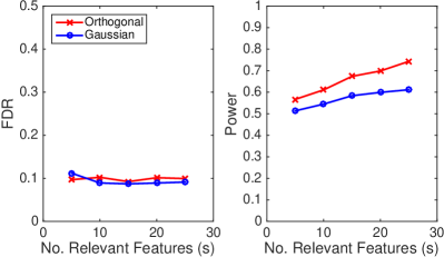
Figure 1: Mean FDR and Power Detecting Signals of Different Sparsity ($s=5,10,15,20,25$).

To show the FDR control property of the ODS (solved with our algorithm), we generated random ODS instances with orthogonal and Gaussian design matrices of the dimension $n=2000$ and $p=1000$, and compared the FDR and the power of the two cases for the target FDR level of $q=0.1$.

Figure 1 shows the mean values of these quality criteria over $300$ repetitions, for increasing numbers of relevant features ($s$) in the true signal (also referred to as signal sparsity). FDR was indeed controlled at the desired level of $10\%$ in both orthogonal and Gaussian cases, as we claimed. We observed slightly improved power with orthogonal design compared to the Gaussian cases: it is natural since $\lambda$ values were adjusted to control FDR resulting in larger penalty for the latter.

Comparing to SLOPE using the same $\lambda$ values under Gaussian design, ODS appeared to be slightly more conservative, improving FDR and the average number of false discoveries at the cost of a small decrease in power (data not shown). So ODS would be appealing for applications like finding biomarkers from high-dimensional genomic data where false positive discoveries can cost much for follow-up validation. We leave more precise comparison to SLOPE as future work.

5.3 Convergence Rate

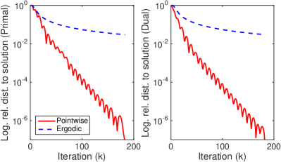
Figure 2: Pointwise and Ergodic Convergence. (Left) Primal; (Right) Dual.

Using our algorithm in experiments, we observed fast pointwise convergence in almost every case. This was quite surprising, since pointwise convergence rate is not explained by the existing analysis in Theorem 1, and also expected to be slow, as we discussed earlier.

Figure 2 shows one instance of the randomly generated Gaussian design cases with $p=n=1000$, $s=15$, and $q=0.1$ (behavior was quite similar in other settings). We ran our algorithm twice for the same data, 1) to obtain the primal and the dual solutions, then 2) to obtain the relative distances of iterates to their corresponding solution, such as $\|{\mathbf{w}}_{k}-{\mathbf{w}}^{*}\|/\|{\mathbf{w}}^{*}\|$.

As we can see, the averaged iterate (denoted by “Ergodic”) showed the expected $O(1/k)$ convergence rate. In contrast, the non-averaged iterates (“pointwise”) converged much faster, even exhibiting typical fluctuation patterns of accelerated gradient method. We believe that this behavior is closely related to the local strong convexity and acceleration we discussed.

In fact, in Figure 2, neither any information of local strong convexity nor the alternative choice of ${\mathbf{v}}^{\prime}_{k+1}=2{\mathbf{v}}_{k+1}$ was used. When the latter option was used, our algorithm showed even faster pointwise convergence, but there were some cases the algorithm did not converge, which would be when the required local strong convexity assumption was not satisfied.

5.4 Local Strong Convexity

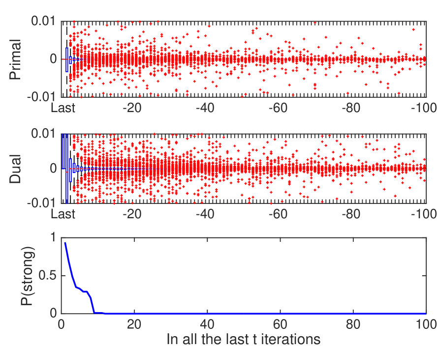
Figure 3: (Top; Middle) Local Strong Convexity Estimates for Primal: ${\mathcal{F}}$ and Dual: ${\mathcal{G}}$ in the last 100 iterations. (Bottom) Probability of Local Strong Convexity in Primal or in Dual, for all of the last $t$ iterations.

We again generated 300 random ODS instances with the same settings as in the previous experiment, to simulate how often the local strong convexity condition (7) would be fulfilled, and to what degree.

Figure 3 (top and middle) reports the box-plots of the local strong convexity estimates:

$$\frac{{\mathcal{F}}({\mathbf{w}}^{*})-{\mathcal{F}}({\mathbf{w}}_{k})-\frac{1}{2}\langle{\mathbf{g}},{\mathbf{w}}^{*}-{\mathbf{w}}_{k}\rangle}{\|{\mathbf{w}}^{*}-{\mathbf{w}}_{k}\|^{2}},\;\;{\mathbf{g}}\in\partial{\mathcal{F}}({\mathbf{w}}_{k}),$$

in the primal, and equivalent quantities regarding ${\mathcal{G}}$ in the dual, evaluated for the last 100 iterations of each run. As we approached the last iteration, these values varied more away from zero, where the chance of being positive was nearly $50\%$ in the primal and dual, resp. In fact, for acceleration to happen, it is very likely from Theorem 2 that the values need to be positive in either primal or dual: Figure 3 (bottom) shows the chance of such events to happen, in all of the last $t$ iterations: the probability seemed to approach one as $t\to 1$. This indicates that local acceleration near an optimal solution would be highly likely.

6 CONCLUSION

We proposed PDSP, a fast and simple primal-dual algorithm to solve the saddle-point formulation of the generalized Dantzig selector. While achieving the known optimal convergence rate, we showed that our algorithm can exhibit a faster rate, taking the advantage of local acceleration. We also introduced the ordered Dantzig selector with FDR control, a new instance of the GDS, which we hope will foster further research in variable selection and signal recovery.

Acknowledgements

SL was supported by Deutsche Forschungsgemeinschaft (DFG) within the Collaborative Research Center SFB 876, project C1. D.B. and M.B. were supported by European Union’s 7th Framework Programme under Grant Agreement no 602552 and by the Polish Ministry of Science and Higher Education under grant agreement 2932/7.PR/2013/2.

Appendix

Proof of Theorem 1

This proof essentially follows that of Chambolle and Pock [2011; Theorem 1], with a small trick to reformulate the GDS-SP to the formulation discussed in the original proof.

From the definition of the proximal steps in Algorithm 1,

$${\mathbf{v}}_{k+1} =(I+\sigma\partial{\mathcal{G}})^{-1}({\mathbf{v}}_{k}+\sigma({\mathbf{X}}^{T}{\mathbf{y}}-{\mathbf{X}}^{T}{\mathbf{X}}{\mathbf{w}}^{\prime}_{k}))$$

$${\mathbf{w}}_{k+1} =(I+\tau\partial{\mathcal{F}})^{-1}({\mathbf{w}}_{k}+\tau{\mathbf{X}}^{T}{\mathbf{X}}{\mathbf{v}}^{\prime}_{k+1}),$$

it is implied that

$$\partial{\mathcal{G}}({\mathbf{v}}_{k+1}) \ni\frac{{\mathbf{v}}_{k}-{\mathbf{v}}_{k+1}}{\sigma}+{\mathbf{X}}^{T}{\mathbf{y}}-{\mathbf{X}}^{T}{\mathbf{X}}{\mathbf{w}}^{\prime}_{k}$$ (11)

$$\partial{\mathcal{F}}({\mathbf{w}}_{k+1}) \ni\frac{{\mathbf{w}}_{k}-{\mathbf{w}}_{k+1}}{\tau}+{\mathbf{X}}^{T}{\mathbf{X}}{\mathbf{v}}^{\prime}_{k+1}.$$

Since ${\mathcal{G}}$ and ${\mathcal{H}}$ are convex functions, it follows for any $({\mathbf{w}},{\mathbf{v}})$,

$${\mathcal{G}}({\mathbf{v}}) \geq{\mathcal{G}}({\mathbf{v}}_{k+1})+\sigma^{-1}\langle{\mathbf{v}}_{k}-{\mathbf{v}}_{k+1},{\mathbf{v}}-{\mathbf{v}}_{k+1}\rangle$$

$$\quad+\langle{\mathbf{X}}^{T}{\mathbf{y}}-{\mathbf{X}}^{T}{\mathbf{X}}{\mathbf{w}}^{\prime}_{k},{\mathbf{v}}-{\mathbf{v}}_{k+1}\rangle$$

$${\mathcal{F}}({\mathbf{w}}) \geq{\mathcal{F}}({\mathbf{w}}_{k+1})+\tau^{-1}\langle{\mathbf{w}}_{k}-{\mathbf{w}}_{k+1},{\mathbf{w}}-{\mathbf{w}}_{k+1}\rangle$$

$$\quad+\langle{\mathbf{X}}^{T}{\mathbf{X}}({\mathbf{w}}-{\mathbf{w}}_{k+1}),{\mathbf{v}}^{\prime}_{k+1}\rangle.$$

We define augmentations of ${\mathbf{w}}$’s with ${\mathbf{y}}$, e.g. ${\mathbf{z}}_{k}:=[{\mathbf{y}};{\mathbf{w}}_{k}]\in\mathbb{R}^{n+p}$, and ${\mathcal{H}}({\mathbf{z}}):={\mathcal{H}}({\mathbf{y}},{\mathbf{w}})={\mathcal{F}}({\mathbf{w}})$. Then the preceding inequalities can be rewritten as follows,

$${\mathcal{G}}({\mathbf{v}}) \geq{\mathcal{G}}({\mathbf{v}}_{k+1})+\sigma^{-1}\langle{\mathbf{v}}_{k}-{\mathbf{v}}_{k+1},{\mathbf{v}}-{\mathbf{v}}_{k+1}\rangle$$ (12)

$$\quad+\langle{\mathbf{A}}{\mathbf{z}}^{\prime}_{k},{\mathbf{v}}-{\mathbf{v}}_{k+1}\rangle$$

$${\mathcal{H}}({\mathbf{z}}) \geq{\mathcal{H}}({\mathbf{z}}_{k+1})+\tau^{-1}\langle{\mathbf{z}}_{k}-{\mathbf{z}}_{k+1},{\mathbf{z}}-{\mathbf{z}}_{k+1}\rangle$$

$$\quad-\langle{\mathbf{A}}({\mathbf{z}}-{\mathbf{z}}_{k+1}),{\mathbf{v}}^{\prime}_{k+1}\rangle.$$

Summing both inequalities and using an elementary result $\langle a-c,b-c\rangle=\|a-c\|^{2}/2+\|b-c\|^{2}/2-\|a-b\|^{2}/2$, we have

$$\frac{\|{\mathbf{v}}-{\mathbf{v}}_{k}\|^{2}}{2\sigma}+\frac{\|{\mathbf{z}}-{\mathbf{z}}_{k}\|^{2}}{2\tau}$$ (13)

$$\;\geq[\langle{\mathbf{A}}{\mathbf{z}}_{k+1},{\mathbf{v}}\rangle-{\mathcal{G}}({\mathbf{v}})+{\mathcal{H}}({\mathbf{z}}_{k+1})]$$

$$\quad-[\langle{\mathbf{A}}{\mathbf{z}},{\mathbf{v}}_{k+1}\rangle-{\mathcal{G}}({\mathbf{v}}_{k+1})+{\mathcal{H}}({\mathbf{z}})]$$

$$\quad+\frac{\|{\mathbf{v}}-{\mathbf{v}}_{k+1}\|^{2}}{2\sigma}+\frac{\|{\mathbf{z}}-{\mathbf{z}}_{k+1}\|^{2}}{2\tau}$$

$$\quad+\frac{\|{\mathbf{v}}_{k}-{\mathbf{v}}_{k+1}\|^{2}}{2\sigma}+\frac{\|{\mathbf{z}}_{k}-{\mathbf{z}}_{k+1}\|^{2}}{2\tau}$$

$$\quad+\langle{\mathbf{A}}({\mathbf{z}}_{k+1}-{\mathbf{z}}^{\prime}_{k}),{\mathbf{v}}_{k+1}-{\mathbf{v}}\rangle$$

$$\quad-\langle{\mathbf{A}}({\mathbf{z}}_{k+1}-{\mathbf{z}}),{\mathbf{v}}_{k+1}-{\mathbf{v}}^{\prime}_{k+1}\rangle.$$

Replacing the extragradient steps,

$$\begin{cases}{\mathbf{z}}^{\prime}_{k}&={\mathbf{z}}_{k}+\theta({\mathbf{z}}_{k}-{\mathbf{z}}_{k-1})\\ {\mathbf{v}}^{\prime}_{k+1}&={\mathbf{v}}_{k+1},\end{cases}$$

the last two lines of (13) can be bounded as follows,

$$\langle{\mathbf{A}}({\mathbf{z}}_{k+1}-{\mathbf{z}}^{\prime}_{k+1},{\mathbf{v}}_{k+1}-{\mathbf{v}}\rangle$$

$$\;\geq\langle{\mathbf{A}}({\mathbf{z}}_{k+1}-{\mathbf{z}}_{k}),{\mathbf{v}}_{k+1}-{\mathbf{v}}\rangle$$

$$\quad-\theta\langle{\mathbf{A}}({\mathbf{z}}_{k}-{\mathbf{z}}_{k-1})),{\mathbf{v}}_{k}-{\mathbf{v}}\rangle$$

$$\quad-\theta L\|{\mathbf{z}}_{k}-{\mathbf{z}}_{k-1}\|\|{\mathbf{v}}_{k+1}-{\mathbf{v}}_{k}\|$$

$$\;\geq\langle{\mathbf{A}}({\mathbf{z}}_{k+1}-{\mathbf{z}}_{k}),{\mathbf{v}}_{k+1}-{\mathbf{v}}\rangle$$

$$\quad-\theta\langle{\mathbf{A}}({\mathbf{z}}_{k}-{\mathbf{z}}_{k-1})),{\mathbf{v}}_{k}-{\mathbf{v}}\rangle$$

$$\quad-\theta^{2}\sqrt{\sigma\tau}L\frac{\|{\mathbf{z}}_{k}-{\mathbf{z}}_{k-1}\|^{2}}{2\tau}-\sqrt{\sigma\tau}L\frac{\|{\mathbf{v}}_{k+1}-{\mathbf{v}}_{k}\|^{2}}{2\sigma}$$

where the first inequality is due to Cauchy-Schwarz and $L:=\|{\mathbf{A}}\|$, and the second is using $|ab|\leq(\alpha/2)a^{2}+1/(2\alpha)b^{2}$ for any $\alpha>0$ (in this case $\alpha=\sqrt{\sigma/\tau}$).

Combining this with the full inequality (13), we have

$$\frac{\|{\mathbf{v}}-{\mathbf{v}}_{k}\|^{2}}{2\sigma}+\frac{\|{\mathbf{z}}-{\mathbf{z}}_{k}\|^{2}}{2\tau}$$

$$\;\geq[\langle{\mathbf{A}}{\mathbf{z}}_{k+1},{\mathbf{v}}\rangle-{\mathcal{G}}({\mathbf{v}})+{\mathcal{H}}({\mathbf{z}}_{k+1})]$$

$$\quad-[\langle{\mathbf{A}}{\mathbf{z}},{\mathbf{v}}_{k+1}\rangle-{\mathcal{G}}({\mathbf{v}}_{k+1})+{\mathcal{H}}({\mathbf{z}})]$$

$$\quad+\frac{\|{\mathbf{v}}-{\mathbf{v}}_{k+1}\|^{2}}{2\sigma}+\frac{\|{\mathbf{z}}-{\mathbf{z}}_{k+1}\|^{2}}{2\tau}$$

$$\quad\left(1-\sqrt{\sigma\tau}L\right)\frac{\|{\mathbf{v}}_{k+1}-{\mathbf{v}}_{k}\|^{2}}{2\sigma}$$

$$\quad+\frac{\|{\mathbf{z}}_{k}-{\mathbf{z}}_{k+1}\|^{2}}{2\tau}-\theta^{2}\sqrt{\sigma\tau}L\frac{\|{\mathbf{z}}_{k}-{\mathbf{z}}_{k-1}\|^{2}}{2\tau}$$

$$\quad+\langle{\mathbf{A}}({\mathbf{z}}_{k+1}-{\mathbf{z}}_{k}),{\mathbf{v}}_{k+1}-{\mathbf{v}}\rangle$$

$$\quad-\theta\langle{\mathbf{A}}({\mathbf{z}}_{k}-{\mathbf{z}}_{k-1})),{\mathbf{v}}_{k}-{\mathbf{v}}\rangle$$

If we choose parameters so that $\theta=1$ and $\sigma\tau L^{2}\leq 1$, and define

$$\Delta_{k}:=\frac{\|{\mathbf{v}}-{\mathbf{v}}_{k}\|^{2}}{2\sigma}+\frac{\|{\mathbf{z}}-{\mathbf{z}}_{k}\|^{2}}{2\tau},$$

it follows that

$$\Delta_{k} \;\geq[\langle{\mathbf{A}}{\mathbf{z}}_{k+1},{\mathbf{v}}\rangle-{\mathcal{G}}({\mathbf{v}})+{\mathcal{H}}({\mathbf{z}}_{k+1})]$$

$$\quad-[\langle{\mathbf{A}}{\mathbf{z}},{\mathbf{v}}_{k+1}\rangle-{\mathcal{G}}({\mathbf{v}}_{k+1})+{\mathcal{H}}({\mathbf{z}})]$$

$$\quad+\Delta_{k+1}$$

$$\quad+\left(1-\sqrt{\sigma\tau}L\right)\frac{\|{\mathbf{v}}_{k+1}-{\mathbf{v}}_{k}\|^{2}}{2\sigma}$$

$$\quad+\frac{\|{\mathbf{z}}_{k}-{\mathbf{z}}_{k+1}\|^{2}}{2\tau}-\sqrt{\sigma\tau}L\frac{\|{\mathbf{z}}_{k}-{\mathbf{z}}_{k-1}\|^{2}}{2\tau}$$

$$\quad+\langle{\mathbf{A}}({\mathbf{z}}_{k+1}-{\mathbf{z}}_{k}),{\mathbf{v}}_{k+1}-{\mathbf{v}}\rangle$$

$$\quad-\langle{\mathbf{A}}({\mathbf{z}}_{k}-{\mathbf{z}}_{k-1})),{\mathbf{v}}_{k}-{\mathbf{v}}\rangle.$$

Summing up the above inequality for $k=0$ to $t-1$, with ${\mathbf{z}}_{-1}={\mathbf{z}}_{0}$ and ${\mathbf{v}}_{-1}={\mathbf{v}}_{0}$, we get

$$\Delta_{0}\geq \sum_{k=1}^{t}\Big{\{}[\langle{\mathbf{A}}{\mathbf{z}}_{k},{\mathbf{v}}\rangle-{\mathcal{G}}({\mathbf{v}})+{\mathcal{H}}({\mathbf{z}}_{k})]$$

$$\quad-[\langle{\mathbf{A}}{\mathbf{z}},{\mathbf{v}}_{k}\rangle-{\mathcal{G}}({\mathbf{v}}_{k})+{\mathcal{H}}({\mathbf{z}})]\Big{\}}$$

$$\;\;+\Delta_{t}$$

$$\quad+\left(1-\sqrt{\sigma\tau}L\right)\sum_{k=1}^{t}\frac{\|{\mathbf{v}}_{k}-{\mathbf{v}}_{k-1}\|^{2}}{2\sigma}$$

$$\quad+\left(1-\sqrt{\sigma\tau}L\right)\sum_{k=1}^{t-1}\frac{\|{\mathbf{z}}_{k}-{\mathbf{z}}_{k-1}\|^{2}}{2\tau}+\frac{\|{\mathbf{z}}_{t}-{\mathbf{z}}_{t-1}\|^{2}}{2\tau}$$

$$\;\;+\langle{\mathbf{A}}({\mathbf{z}}_{t}-{\mathbf{z}}_{t-1}),{\mathbf{v}}_{t}-{\mathbf{v}}\rangle$$

$$\geq \sum_{k=1}^{t}\Big{\{}[\langle{\mathbf{A}}{\mathbf{z}}_{k},{\mathbf{v}}\rangle-{\mathcal{G}}({\mathbf{v}})+{\mathcal{H}}({\mathbf{z}}_{k})]$$

$$\quad-[\langle{\mathbf{A}}{\mathbf{z}},{\mathbf{v}}_{k}\rangle-{\mathcal{G}}({\mathbf{v}}_{k})+{\mathcal{H}}({\mathbf{z}})]\Big{\}}$$

$$\;\;+\Delta_{t}$$

$$\quad+\left(1-\sqrt{\sigma\tau}L\right)\sum_{k=1}^{t}\frac{\|{\mathbf{v}}_{k}-{\mathbf{v}}_{k-1}\|^{2}}{2\sigma}$$

$$\quad+\left(1-\sqrt{\sigma\tau}L\right)\sum_{k=1}^{t-1}\frac{\|{\mathbf{z}}_{k}-{\mathbf{z}}_{k-1}\|^{2}}{2\tau}+\frac{\|{\mathbf{z}}_{t}-{\mathbf{z}}_{t-1}\|^{2}}{2\tau}$$

$$\;\;-\frac{\|{\mathbf{z}}_{t}-{\mathbf{z}}_{t-1}\|^{2}}{2\tau}-\tau L^{2}\frac{\|{\mathbf{v}}_{t}-{\mathbf{v}}\|^{2}}{2}.$$

That is, for any $({\mathbf{z}},{\mathbf{v}})$,

$$(1-\tau\sigma L^{2})\frac{\|{\mathbf{v}}-{\mathbf{v}}_{t}\|^{2}}{\sigma}+\frac{\|{\mathbf{z}}-{\mathbf{z}}_{t}\|^{2}}{\tau}$$ (14)

$$\quad+2\sum_{k=1}^{t}\Big{\{}[\langle{\mathbf{A}}{\mathbf{z}}_{k},{\mathbf{v}}\rangle-{\mathcal{G}}({\mathbf{v}})+{\mathcal{H}}({\mathbf{z}}_{k})]$$

$$\quad-[\langle{\mathbf{A}}{\mathbf{z}},{\mathbf{v}}_{k}\rangle-{\mathcal{G}}({\mathbf{v}}_{k})+{\mathcal{H}}({\mathbf{z}})]\Big{\}}$$

$$\quad+\left(1-\sqrt{\sigma\tau}L\right)\sum_{k=1}^{t}\frac{\|{\mathbf{v}}_{k}-{\mathbf{v}}_{k-1}\|^{2}}{\sigma}$$

$$\quad+\left(1-\sqrt{\sigma\tau}L\right)\sum_{k=1}^{t-1}\frac{\|{\mathbf{z}}_{k}-{\mathbf{z}}_{k-1}\|^{2}}{\tau}$$

$$\leq\frac{\|{\mathbf{v}}-{\mathbf{v}}_{0}\|^{2}}{\sigma}+\frac{\|{\mathbf{z}}-{\mathbf{z}}_{0}\|^{2}}{\tau}.$$

For any saddle point $({\mathbf{z}}^{*},{\mathbf{v}}^{*})$ satisfying the conditions in (5), we observe that

$$[\langle{\mathbf{A}}{\mathbf{z}}_{k},{\mathbf{v}}^{*}\rangle-{\mathcal{G}}({\mathbf{v}}^{*})+{\mathcal{H}}({\mathbf{z}}_{k})]$$ (15)

$$\;\;\geq[\langle{\mathbf{A}}{\mathbf{z}}^{*},{\mathbf{v}}^{*}\rangle-{\mathcal{G}}({\mathbf{v}}^{*})+{\mathcal{H}}({\mathbf{z}}^{*})]$$

$$\;\;\geq[\langle{\mathbf{A}}{\mathbf{z}}^{*},{\mathbf{v}}_{k}\rangle-{\mathcal{G}}({\mathbf{v}}_{k})+{\mathcal{H}}({\mathbf{z}}^{*})].$$

That is, for $({\mathbf{z}},{\mathbf{v}})=({\mathbf{z}}^{*},{\mathbf{v}}^{*})$ the first summation in (14) is non-negative, and therefore $({\mathbf{z}}_{k},{\mathbf{v}}_{k})$ is bounded, showing the property (a).

Also, from (14) due the convexity of ${\mathcal{G}}$ and ${\mathcal{H}}$, we have the following result for $\overline{\mathbf{z}}_{t}=\frac{1}{t}\sum_{k=1}^{t}{\mathbf{z}}_{k}$ and $\overline{\mathbf{v}}_{t}=\frac{1}{t}\sum_{k=1}^{t}{\mathbf{v}}_{k}$,

$$[\langle{\mathbf{A}}\overline{\mathbf{z}}_{t},{\mathbf{v}}\rangle-{\mathcal{G}}({\mathbf{v}})+{\mathcal{H}}(\overline{\mathbf{z}}_{t})]-[\langle{\mathbf{A}}{\mathbf{z}},\overline{\mathbf{v}}_{t}\rangle-{\mathcal{G}}(\overline{\mathbf{v}}_{t})+{\mathcal{H}}({\mathbf{z}})]$$ (16)

$$\;\;\leq\frac{1}{t}\left(\frac{\|{\mathbf{v}}-{\mathbf{v}}_{0}\|^{2}}{2\sigma}+\frac{\|{\mathbf{z}}-{\mathbf{z}}_{0}\|^{2}}{2\tau}\right)$$

$$\;\;\leq\frac{1}{t}\left(\frac{\|{\mathbf{v}}-{\mathbf{v}}^{*}\|^{2}}{2\sigma}+\frac{\|{\mathbf{v}}^{*}-{\mathbf{v}}_{0}\|^{2}}{2\sigma}\right.$$

$$\quad+\left.\frac{\|{\mathbf{z}}-{\mathbf{z}}^{*}\|^{2}}{2\tau}+\frac{\|{\mathbf{z}}^{*}-{\mathbf{z}}_{0}\|^{2}}{2\tau}\right)$$

$$\;\;\leq\frac{1+C}{t}\left(\frac{\|{\mathbf{v}}^{*}-{\mathbf{v}}_{0}\|^{2}}{2\sigma}+\frac{\|{\mathbf{z}}^{*}-{\mathbf{z}}_{0}\|^{2}}{2\tau}\right),$$

where $C=1/(1-\tau\sigma L^{2})$ and the last inequality is due to the previous result (a). This shows the first part of (b).

Furthermore, with $t\to\infty$, (16) implies for any limit point $(\hat{\mathbf{z}},\hat{\mathbf{v}})$ of $(\overline{\mathbf{z}}_{t},\overline{\mathbf{v}}_{t})$ that

$$[\langle{\mathbf{A}}\hat{\mathbf{z}},{\mathbf{v}}\rangle-{\mathcal{G}}({\mathbf{v}})+{\mathcal{H}}(\hat{\mathbf{z}})]-[\langle{\mathbf{A}}{\mathbf{z}},\hat{\mathbf{v}}\rangle-{\mathcal{G}}(\hat{\mathbf{v}})+{\mathcal{H}}({\mathbf{z}})]\leq 0$$

since ${\mathcal{H}}$ and ${\mathcal{G}}$ are l.s.c., i.e.

$$\liminf_{t\to\infty}{\mathcal{H}}(\overline{\mathbf{z}}_{t})\geq{\mathcal{H}}(\hat{\mathbf{z}}),\;\;\liminf_{t\to\infty}{\mathcal{G}}(\overline{\mathbf{v}}_{t})\geq{\mathcal{G}}(\hat{\mathbf{v}}).$$

This implies that $(\hat{\mathbf{z}},\hat{\mathbf{v}})$ is a saddle-point of (4), the second claim in (b).

Finally, since $(1-\sqrt{\sigma\tau}L)\geq 0$, (14) also implies that $\|{\mathbf{v}}_{k}-{\mathbf{v}}_{k-1}\|\to 0$ and $\|{\mathbf{z}}_{k}-{\mathbf{z}}_{k-1}\|\to 0$ as $k\to\infty$, and therefore $({\mathbf{z}}_{k},{\mathbf{v}}_{k})$ should have a limit, say $(\tilde{\mathbf{z}},\tilde{\mathbf{v}})$. Then again from (14), we have at the limit

$$[\langle{\mathbf{A}}\tilde{z},{\mathbf{v}}^{*}\rangle-{\mathcal{G}}({\mathbf{v}}^{*})+{\mathcal{H}}(\tilde{z})]-[\langle{\mathbf{A}}{\mathbf{z}}^{*},\tilde{\mathbf{v}}\rangle-{\mathcal{G}}(\tilde{\mathbf{v}})+{\mathcal{H}}({\mathbf{z}}^{*})]=0,$$

which tells that $(\tilde{\mathbf{z}},\tilde{\mathbf{v}})$ is also a saddle-point, showing the last claim (c). ∎

Proof of Theorem 2

Hence ${\mathcal{F}}$ satisfies the local strong convexity (7), so does the function ${\mathcal{H}}({\mathbf{z}})={\mathcal{H}}({\mathbf{y}},{\mathbf{w}})={\mathcal{F}}({\mathbf{w}})$ on augmented vectors ${\mathbf{z}}=({\mathbf{y}},{\mathbf{w}})$, and from the expression of subgradients (11) we have (with $\tau^{\prime}_{k}=2\tau_{k}$)

$${\mathcal{H}}({\mathbf{z}}^{*}) \geq{\mathcal{H}}({\mathbf{z}}_{k+1})+\left\langle\frac{{\mathbf{z}}_{k}-{\mathbf{z}}_{k+1}}{\tau^{\prime}_{k}},{\mathbf{z}}^{*}-{\mathbf{z}}_{k+1}\right\rangle$$

$$-\left\langle{\mathbf{A}}({\mathbf{z}}^{*}-{\mathbf{z}}_{k+1}),\frac{{\mathbf{v}}^{\prime}_{k+1}}{2}\right\rangle+\frac{\delta}{2}\|{\mathbf{z}}^{*}-{\mathbf{z}}_{k+1}\|^{2}.$$

Also, from the convexity of ${\mathcal{G}}$ (12),

$${\mathcal{G}}({\mathbf{v}}^{*}) \geq{\mathcal{G}}({\mathbf{v}}_{k+1})+\left\langle\frac{{\mathbf{v}}_{k}-{\mathbf{v}}_{k+1}}{\sigma_{k}},{\mathbf{v}}^{*}-{\mathbf{v}}_{k+1}\right\rangle$$

$$\quad+\langle{\mathbf{A}}{\mathbf{z}}^{\prime}_{k},{\mathbf{v}}^{*}-{\mathbf{v}}_{k+1}\rangle.$$

With these, the previous inequality (13) modifies as follows,

$$\frac{\|{\mathbf{v}}^{*}-{\mathbf{v}}_{k}\|^{2}}{2\sigma_{k}}+\frac{\|{\mathbf{z}}^{*}-{\mathbf{z}}_{k}\|^{2}}{2\tau^{\prime}_{k}}$$

$$\;\geq[\langle{\mathbf{A}}{\mathbf{z}}_{k+1},{\mathbf{v}}^{*}\rangle-{\mathcal{G}}({\mathbf{v}}^{*})+{\mathcal{H}}({\mathbf{z}}_{k+1})]$$

$$\quad-[\langle{\mathbf{A}}{\mathbf{z}}^{*},{\mathbf{v}}_{k+1}\rangle-{\mathcal{G}}({\mathbf{v}}_{k+1})+{\mathcal{H}}({\mathbf{z}}^{*})]$$

$$\quad+\frac{\delta}{2}\|{\mathbf{z}}^{*}-{\mathbf{z}}_{k+1}\|^{2}+\frac{\|{\mathbf{v}}^{*}-{\mathbf{v}}_{k+1}\|^{2}}{2\sigma_{k}}+\frac{\|{\mathbf{z}}^{*}-{\mathbf{z}}_{k+1}\|^{2}}{2\tau^{\prime}_{k}}$$

$$\quad+\frac{\|{\mathbf{v}}_{k}-{\mathbf{v}}_{k+1}\|^{2}}{2\sigma_{k}}+\frac{\|{\mathbf{z}}_{k}-{\mathbf{z}}_{k+1}\|^{2}}{2\tau^{\prime}_{k}}$$

$$\quad+\langle{\mathbf{A}}({\mathbf{z}}_{k+1}-{\mathbf{z}}^{\prime}_{k}),{\mathbf{v}}_{k+1}-{\mathbf{v}}^{*}\rangle$$

$$\quad-\langle{\mathbf{A}}({\mathbf{z}}_{k+1}-{\mathbf{z}}^{*}),{\mathbf{v}}_{k+1}-\frac{{\mathbf{v}}^{\prime}_{k+1}}{2}\rangle.$$

From (15), the expression in the first two terms of the right-hand side is bounded below by zero.

Choosing the extragradient steps as follows,

$$\begin{cases}{\mathbf{z}}^{\prime}_{k}&={\mathbf{z}}_{k}+\theta_{k-1}({\mathbf{z}}_{k}-{\mathbf{z}}_{k-1})\\ {\mathbf{v}}^{\prime}_{k+1}&=2{\mathbf{v}}_{k+1},\end{cases}$$

it follows that

$$\frac{\|{\mathbf{v}}^{*}-{\mathbf{v}}_{k}\|^{2}}{2\sigma_{k}}+\frac{\|{\mathbf{z}}^{*}-{\mathbf{z}}_{k}\|^{2}}{2\tau^{\prime}_{k}}$$

$$\;\geq\frac{\delta}{2}\|{\mathbf{z}}^{*}-{\mathbf{z}}_{k+1}\|^{2}+\frac{\|{\mathbf{v}}^{*}-{\mathbf{v}}_{k+1}\|^{2}}{2\sigma_{k}}+\frac{\|{\mathbf{z}}^{*}-{\mathbf{z}}_{k+1}\|^{2}}{2\tau^{\prime}_{k}}$$

$$\quad+\frac{\|{\mathbf{v}}_{k}-{\mathbf{v}}_{k+1}\|^{2}}{2\sigma_{k}}+\frac{\|{\mathbf{z}}_{k}-{\mathbf{z}}_{k+1}\|^{2}}{2\tau^{\prime}_{k}}$$

$$\quad+\langle{\mathbf{A}}({\mathbf{z}}_{k+1}-{\mathbf{z}}_{k}),{\mathbf{v}}_{k+1}-{\mathbf{v}}^{*}\rangle$$

$$\quad-\theta_{k-1}\langle{\mathbf{A}}({\mathbf{z}}_{k}-{\mathbf{z}}_{k-1}),{\mathbf{v}}_{k}-{\mathbf{v}}^{*}\rangle$$

$$\quad-\theta_{k-1}L\|{\mathbf{z}}_{k}-{\mathbf{z}}_{k-1}\|\|{\mathbf{v}}_{k+1}-{\mathbf{v}}_{k}\|.$$

The rest of the proof is very similar to that of Section 5 of Chambolle and Pock [2011], from eq. (39) to (42) therein. From the above, we have

$$\frac{\|{\mathbf{v}}^{*}-{\mathbf{v}}_{k}\|^{2}}{\sigma_{k}}+\frac{\|{\mathbf{z}}^{*}-{\mathbf{z}}_{k}\|^{2}}{\tau^{\prime}_{k}}$$

$$\;\geq(1+\delta\tau^{\prime}_{k})\frac{\tau^{\prime}_{k+1}}{\tau^{\prime}_{k}}\frac{\|{\mathbf{z}}^{*}-{\mathbf{z}}_{k+1}\|^{2}}{\tau^{\prime}_{k+1}}+\frac{\sigma_{k+1}}{\sigma_{k}}\frac{\|{\mathbf{v}}^{*}-{\mathbf{v}}_{k+1}\|^{2}}{\sigma_{k+1}}$$

$$\quad+\frac{\|{\mathbf{v}}_{k}-{\mathbf{v}}_{k+1}\|^{2}}{\sigma_{k}}+\frac{\|{\mathbf{z}}_{k}-{\mathbf{z}}_{k+1}\|^{2}}{\tau^{\prime}_{k}}-\frac{\|{\mathbf{v}}_{k+1}-{\mathbf{v}}_{k}\|^{2}}{\sigma_{k}}$$

$$\quad+2\langle{\mathbf{A}}({\mathbf{z}}_{k+1}-{\mathbf{z}}_{k}),{\mathbf{v}}_{k+1}-{\mathbf{v}}^{*}\rangle$$

$$\quad-2\theta_{k-1}\langle{\mathbf{A}}({\mathbf{z}}_{k}-{\mathbf{z}}_{k-1}),{\mathbf{v}}_{k}-{\mathbf{v}}^{*}\rangle$$

$$\quad-\theta_{k-1}^{2}L^{2}\sigma_{k}\tau^{\prime}_{k-1}\frac{\|{\mathbf{z}}_{k}-{\mathbf{z}}_{k-1}\|^{2}}{\tau^{\prime}_{k-1}}.$$

We choose sequences $\tau^{\prime}_{k}$ and $\sigma_{k}$ such that

$$(1+\delta\tau^{\prime}_{k})\frac{\tau^{\prime}_{k+1}}{\tau^{\prime}_{k}}=\frac{\sigma_{k+1}}{\sigma_{k}}=\frac{1}{\theta_{k}}=\frac{\tau^{\prime}_{k}}{\tau^{\prime}_{k+1}}>1.$$

Denoting

$$\Delta_{k}:=\frac{\|{\mathbf{v}}^{*}-{\mathbf{v}}_{k}\|^{2}}{\sigma_{k}}+\frac{\|{\mathbf{z}}^{*}-{\mathbf{z}}_{k}\|^{2}}{\tau^{\prime}_{k}},$$

dividing the both sides of the above inequality by $\tau^{\prime}_{k}$, and using $L^{2}\sigma_{k}\tau^{\prime}_{k}=L^{2}\sigma_{0}\tau^{\prime}_{0}\leq 1$, we get

$$\frac{\Delta_{k}}{\tau^{\prime}_{k}}\geq\frac{\Delta_{k+1}}{\tau^{\prime}_{k+1}}+\frac{\|{\mathbf{z}}_{k}-{\mathbf{z}}_{k+1}\|^{2}}{(\tau^{\prime}_{k})^{2}}-\frac{\|{\mathbf{z}}_{k}-{\mathbf{z}}_{k-1}\|^{2}}{(\tau^{\prime}_{k-1})^{2}}$$

$$\quad+\frac{2}{\tau^{\prime}_{k}}\langle{\mathbf{A}}({\mathbf{z}}_{k+1}-{\mathbf{z}}_{k}),{\mathbf{v}}_{k+1}-{\mathbf{v}}^{*}\rangle$$

$$\quad-\frac{2}{\tau^{\prime}_{k-1}}\langle{\mathbf{A}}({\mathbf{z}}_{k}-{\mathbf{z}}_{k-1}),{\mathbf{v}}_{k}-{\mathbf{v}}^{*}\rangle.$$

Applying this inequality for $k=0,\cdots,(t-1)$, and using ${\mathbf{z}}_{-1}={\mathbf{z}}_{0}$, it leads to

$$\frac{\Delta_{0}}{\tau^{\prime}_{0}} \geq\frac{\Delta_{t}}{\tau^{\prime}_{t}}+\frac{\|{\mathbf{z}}_{t-1}-{\mathbf{z}}_{t}\|^{2}}{(\tau^{\prime}_{t-1})^{2}}$$

$$\quad+\frac{2}{\tau^{\prime}_{t-1}}\langle{\mathbf{A}}({\mathbf{z}}_{t}-{\mathbf{z}}_{t-1}),{\mathbf{v}}_{t}-{\mathbf{v}}^{*}\rangle$$

$$\geq\frac{\Delta_{t}}{\tau^{\prime}_{t}}+\frac{\|{\mathbf{z}}_{t-1}-{\mathbf{z}}_{t}\|^{2}}{(\tau^{\prime}_{t-1})^{2}}$$

$$\quad-\frac{\|{\mathbf{z}}_{t}-{\mathbf{z}}_{t-1}\|^{2}}{(\tau^{\prime}_{t-1})^{2}}-L^{2}\|{\mathbf{v}}_{t}-{\mathbf{v}}^{*}\|^{2}.$$

Rearranging terms, using $L^{2}\sigma_{k}\tau^{\prime}_{k}=L^{2}\sigma_{0}\tau^{\prime}_{0}$, and replacing $\tau^{\prime}_{k}=2\tau_{k}$, we finally obtain

$$4\tau_{t}^{2}\frac{1-2L^{2}\sigma_{0}\tau_{0}}{2\sigma_{0}\tau_{0}}\|{\mathbf{v}}^{*}-{\mathbf{v}}_{t}\|^{2}+\|{\mathbf{z}}^{*}-{\mathbf{z}}_{t}\|^{2}$$

$$\leq 4\tau_{t}^{2}\left(\frac{\|{\mathbf{z}}^{*}-{\mathbf{z}}_{0}\|^{2}}{4\tau_{0}^{2}}+\frac{\|{\mathbf{v}}^{*}-{\mathbf{v}}_{0}\|^{2}}{2\sigma_{0}\tau_{0}}\right).$$

If we choose $\sigma_{0},\tau_{0}$ so that $2\sigma_{0}\tau_{0}L^{2}=1$, then

$$\|{\mathbf{z}}^{*}-{\mathbf{z}}_{t}\|^{2}\leq 4\tau_{t}^{2}\left(\frac{\|{\mathbf{z}}^{*}-{\mathbf{z}}_{0}\|^{2}}{4\tau_{0}^{2}}+L^{2}\|{\mathbf{v}}^{*}-{\mathbf{v}}_{0}\|^{2}\right).$$

The proof completes if we show $\tau_{t}\sim t^{-1}$ for all $t\geq t_{0}$. Note that our choice of $\tau_{k}$ satisfies (with $\tau^{\prime}_{k}=2\tau_{k}$),

$$(1+2\delta\tau_{k})\frac{\tau_{k+1}}{\tau_{k}}=\frac{\tau_{k}}{\tau_{k+1}},$$

which is an identical choice to that of Lemma 1 of Chambolle and Pock [2011], replacing $\gamma=\delta$ therein. Therefore Corollary 1 of Chambolle and Pock [2011] applies as it is, which shows that $\lim_{t\to\infty}t\delta\tau_{t}=1$. ∎

FDR Control of the ODS

Properties of $J_{\boldsymbol{\lambda}}$ and $J_{\boldsymbol{\lambda}}^{D}$

Proposition 1.

If ${\mathbf{a}}$, ${\mathbf{b}}\in\mathbb{R}^{p}$ are such that $|{\mathbf{a}}|\preceq|{\mathbf{b}}|$, then the vectors sorted in decreasing component magnitudes satisfy $|{\mathbf{a}}|_{(\cdot)}\preceq|{\mathbf{b}}|_{(\cdot)}$.

Proof.

Without loss of generality assume that ${\mathbf{a}}$ and ${\mathbf{b}}$ are nonnegative and that $a_{1}\geq\ldots\geq a_{p}$. We will show that $a_{k}\leq b_{(k)}$ for $k\in\{1,\ldots,p\}$. Fix such $k$ and consider the set $S_{k}:=\{b_{i}:\ b_{i}\geq a_{k}\}$. It is enough to show that $|S_{k}|\geq k$, where $|S_{k}|$ is the number of elements in $S_{k}$. For each $j\in\{1,\ldots,k\}$ we have

$$b_{j}\geq a_{j}\geq a_{k}\ \Longrightarrow\ b_{j}\in S_{k},$$

what proves the last statement. ∎

Corollary 1.

Let ${\mathbf{a}},{\mathbf{b}}\in\mathbb{R}^{p}$ and $|{\mathbf{a}}|\preceq|{\mathbf{b}}|$. Then ${J_{\boldsymbol{\lambda}}({\mathbf{a}})\leq J_{\boldsymbol{\lambda}}({\mathbf{b}})}$ since $J_{\boldsymbol{\lambda}}({\mathbf{a}})={\boldsymbol{\lambda}}^{T}|{\mathbf{a}}|_{(\cdot)}\leq{\boldsymbol{\lambda}}^{T}|{\mathbf{b}}|_{(\cdot)}=J_{\boldsymbol{\lambda}}({\mathbf{b}})$.

Proposition 2 (Pulling to zero).

For fixed sequence $\lambda_{1}\geq\ldots\geq\lambda_{p}\geq 0$, let ${\mathbf{w}}\in\mathbb{R}^{p}$ be such that $w_{j}>0$ for some ${j\in\{1,\ldots,p\}}$. For $\varepsilon\in(0,w_{j}]$ define:

$$(w_{\varepsilon})_{i}=\left\{\begin{array}[]{ll}w_{j}-\varepsilon,&i=j\\ w_{i},&\textrm{otherwise}\end{array}\right..$$

Then:
(i) $J_{\lambda}({\mathbf{w}}_{\varepsilon})\leq J_{\lambda}({\mathbf{w}})$,
(ii) if ${\boldsymbol{\lambda}}\succ 0$, then $J_{\lambda}({\mathbf{w}}_{\varepsilon})<J_{\lambda}({\mathbf{w}}).$

Proof.

Let $\pi:\{1,\ldots,p\}\longrightarrow\{1,\ldots,p\}$ be permutation such as $\sum_{i=1}^{p}\lambda_{i}(w_{\varepsilon})_{(i)}=\sum_{i=1}^{p}\lambda_{\pi(i)}(w_{\varepsilon})_{i}$ for each $i$ in $\{1,\ldots,p\}$. Using the rearrangement inequality [Hardy et al., 1994]

$$J_{\boldsymbol{\lambda}}({\mathbf{w}})-J_{\boldsymbol{\lambda}}({\mathbf{w}}_{\varepsilon})=\sum_{i=1}^{p}\lambda_{i}w_{(i)}-\sum_{i=1}^{p}\lambda_{\pi(i)}(w_{\varepsilon})_{i}$$

$$\geq\sum_{i=1}^{p}\lambda_{\pi(i)}w_{i}-\sum_{i=1}^{p}\lambda_{\pi(i)}(w_{\varepsilon})_{i}=\varepsilon\lambda_{\pi(j)}\geq 0.$$

If ${\boldsymbol{\lambda}}\succ 0$, then the last inequality is strict. ∎

Proposition 3 (Pulling to the mean).

For fixed sequence $\lambda_{1}\geq\ldots\geq\lambda_{p}\geq 0$, let ${\mathbf{w}}\in\mathbb{R}^{p}$ be such that ${\mathbf{w}}\succeq 0$ and $w_{j}>w_{l}$ for some ${j,l\in\{1,\ldots,p\}}$. For $0<\varepsilon\leq\frac{w_{j}-w_{l}}{2}$ define:

$$(w_{\varepsilon})_{i}=\left\{\begin{array}[]{ll}w_{l}+\varepsilon,&i=l\\ w_{j}-\varepsilon,&i=j\\ w_{i},&\textrm{otherwise}\end{array}\right..$$

Then:
(i) $J_{\boldsymbol{\lambda}}({\mathbf{w}}_{\varepsilon})\leq J_{\boldsymbol{\lambda}}({\mathbf{w}})$,
(ii) if $\lambda_{1}>\ldots>\lambda_{p}$, then $J_{\boldsymbol{\lambda}}({\mathbf{w}}_{\varepsilon})<J_{\boldsymbol{\lambda}}({\mathbf{w}}).$

Proof.

Let $\pi:\{1,\ldots,p\}\longrightarrow\{1,\ldots,p\}$ be permutation such as $\sum_{i=1}^{p}\lambda_{i}(w_{\varepsilon})_{(i)}=\sum_{i=1}^{p}\lambda_{\pi(i)}(w_{\varepsilon})_{i}$ for each $i$ in $\{1,\ldots,p\}$ and $\lambda_{\pi(j)}\geq\lambda_{\pi(l)}$. From the rearrangement inequality,

$$J_{\boldsymbol{\lambda}}({\mathbf{w}})-J_{\boldsymbol{\lambda}}({\mathbf{w}}_{\varepsilon})$$

$$=\sum_{i=1}^{p}\lambda_{i}w_{(i)}-\sum_{i=1}^{p}\lambda_{i}(w_{\varepsilon})_{(i)}$$

$$=\sum_{i=1}^{p}\lambda_{i}w_{(i)}-\sum_{i=1}^{p}\lambda_{\pi(i)}(w_{\varepsilon})_{i}$$

$$\geq\sum_{i=1}^{p}\lambda_{\pi(i)}w_{i}-\sum_{i=1}^{p}\lambda_{\pi(i)}(w_{\varepsilon})_{i}$$

$$=\varepsilon\big{(}\lambda_{\pi(j)}-\lambda_{\pi(l)}\big{)}\geq 0.$$

If $\lambda_{1}>\ldots>\lambda_{p}$, then the last inequality is strict. ∎

Proposition 4.

Suppose that $\lambda_{1}\geq\ldots\geq\lambda_{p}\geq 0$. For arbitrary ${\mathbf{x}}\in\mathbb{R}^{p}$, $\varepsilon>0$, and $l,j\in\{1,\dots,p\}$ define:

$$(x_{\varepsilon})_{i} =\left\{\begin{array}[]{ll}x_{l}+\varepsilon,&i=l\\ x_{j}-\varepsilon,&i=j\\ x_{i},&\textrm{otherwise}\end{array}\right.,$$

$$(\widetilde{x}_{\varepsilon})_{i} =\left\{\begin{array}[]{ll}x_{j}-\varepsilon,&i=j\\ x_{i},&\textrm{otherwise}\end{array}\right..$$

Then:
i) if $x_{j}>x_{l}\geq 0$, then for $\varepsilon\in\big{(}0,(x_{j}-x_{l})/2\big{]}$ it holds that $J_{\boldsymbol{\lambda}}^{D}({\mathbf{x}}_{\varepsilon})\leq J_{\boldsymbol{\lambda}}^{D}({\mathbf{x}})$,
ii) if $x_{j}>0$, then for $\varepsilon\in\big{(}0,x_{j}\big{]}$ it holds $J_{\boldsymbol{\lambda}}^{D}(\widetilde{{\mathbf{x}}}_{\varepsilon})\leq J_{\boldsymbol{\lambda}}^{D}({\mathbf{x}})$.

Proof.

It is easy to observe that for any ${\mathbf{x}}\in\mathbb{R}^{p}$, the dual to the sorted $\ell_{1}$-norm could be represented as ${J_{\boldsymbol{\lambda}}^{D}({\mathbf{x}})=\max\Big{\{}J_{\lambda^{k}}(x),\ k\leq p\Big{\}}}$ for

$$\lambda^{k}_{i}:=\left\{\begin{array}[]{cl}\big{(}\sum_{j=1}^{k}\lambda_{j}\big{)}^{-1},&i\leq k\\ 0,&\textrm{otherwise}\end{array}\right..$$

The claim is therefore the straightforward consequence of Propositions 2 and 3. ∎

Proposition 5.

If $|{\mathbf{w}}|\preceq|\widetilde{{\mathbf{w}}}|$, then $J_{\boldsymbol{\lambda}}^{D}({\mathbf{w}})\leq J_{\boldsymbol{\lambda}}^{D}(\widetilde{{\mathbf{w}}})$.

Proof.

Claim follows simply from Corollary 1, analogously as in proof of previous proposition. ∎

Properties of the ODS with an Orthogonal Design

Before proving Theorem 3, we will recall results concerning the SLOPE problem,

$$\min_{{\mathbf{w}}}\;\;\frac{1}{2}\|{\mathbf{y}}-{\mathbf{X}}{\mathbf{w}}\|^{2}+J_{\boldsymbol{\lambda}}({\mathbf{w}}).$$ (17)

and derive some properties useful in analysis of the ODS problem (8). Since $\frac{1}{2}\big{\|}{\mathbf{y}}-{\mathbf{X}}{\mathbf{w}}\big{\|}_{2}^{2}=\frac{1}{2}\big{\|}\widetilde{{\mathbf{y}}}-{\mathbf{w}}\big{\|}_{2}^{2}+const$ and ${\mathbf{X}}^{T}({\mathbf{y}}-{\mathbf{X}}{\mathbf{w}})=\widetilde{{\mathbf{y}}}-{\mathbf{w}}$ under orthogonal design, for $\widetilde{{\mathbf{y}}}:={\mathbf{X}}^{T}{\mathbf{y}}$, without loss of generality we will consider the case ${\mathbf{X}}=\mathbf{I}_{p}$ (hereafter we also denote $\tilde{\mathbf{y}}$ by ${\mathbf{y}}$ to simplify notations). Let $I_{1}$ be some subset of $\{1,\ldots,p\}$ and $\overline{{\mathbf{w}}_{I_{1}}}$ denotes the arithmetic mean of subvector ${\mathbf{w}}_{I_{1}}$, for any ${\mathbf{w}}\in\mathbb{R}^{p}$. Bogdan et al. [2015] showed that the unique solution to (17) (uniqueness follows from strict convexity of objective function) is output of the following Algorithm 2, which terminates in at most $n$ steps.

Input: Nonnegative and nonincreasing sequences $y$ and $\lambda$;

while ${\mathbf{y}}-{\boldsymbol{\lambda}}$ is not nonincreasing do

       Identify strictly increasing subsequences, i.e. segments $I_{i}:=\{j,\ldots,l\}$ such that

$$y_{j}-\lambda_{j}<\ldots<y_{l}-\lambda_{l}.$$

For each $k\in I_{i}$ replace the values of $y$ and $\lambda$ by their average value over such segments

$$y_{k}\leftarrow\overline{y_{I_{i}}},\qquad\lambda_{k}\leftarrow\overline{\lambda_{I_{i}}}$$

end while

output: ${\mathbf{w}}_{S}=({\mathbf{y}}-{\boldsymbol{\lambda}})_{+}$;

Algorithm 2 Solution to SLOPE in the Orthogonal Case [Bogdan et al., 2015; Algorithm 3]

The same authors showed that (17) can be casted as a quadratic program,

$$\begin{array}[]{cl}\min_{{\mathbf{w}}\in\mathbb{R}^{p}}&\ \frac{1}{2}\|{\mathbf{y}}-{\mathbf{w}}\|_{2}^{2}+{\boldsymbol{\lambda}}^{T}{\mathbf{w}}\\[2.84544pt] \textrm{subject to}&\begin{array}[]{l}w_{1}\geq\ldots\geq w_{p}\geq 0\end{array}.\end{array}$$

We aim to show that the ODS (8) can be reformulated as a linear program, and then to show that its solution is unique and can be given by the same Algorithm 2 for SLOPE.

Taking into account that ${\mathbf{X}}=\mathbf{I}_{p}$, the ODS for the orthogonal design can be rewritten as

$$\min_{\mathbf{w}}\ J_{\boldsymbol{\lambda}}({\mathbf{w}})\quad\textrm{subject to}\quad{\mathbf{y}}-{\mathbf{w}}\in C_{{\boldsymbol{\lambda}}},$$ (18)

where $C_{\boldsymbol{\lambda}}$ is the unit ball in terms of the dual norm, $J_{\boldsymbol{\lambda}}^{D}$. It is easy to see that if ${\mathbf{y}}-{\mathbf{w}}\in C_{\boldsymbol{\lambda}}$, then also ${\mathbf{P}}_{\pi}({\mathbf{y}}-{\mathbf{w}})\in C_{\boldsymbol{\lambda}}$ and ${\mathbf{S}}({\mathbf{y}}-{\mathbf{w}})\in C_{\boldsymbol{\lambda}}$ for any permutation $\pi$ and diagonal matrix ${\mathbf{S}}$ with $|S_{ii}|=1$, $i=1,\ldots,p$.

Proposition 6.

Suppose that ${\mathbf{w}}^{*}$ is solution to (18), $\pi$ is arbitrary permutation of $\{1,\ldots,p\}$ and ${\mathbf{S}}$ is diagonal matrix such as $|S_{ii}|=1$ for all $i$. Then
i) ${\mathbf{w}}^{*}_{\pi}:={\mathbf{P}}_{\pi}{\mathbf{w}}^{*}$ is a solution to

$$\min_{\mathbf{w}}J_{\boldsymbol{\lambda}}({\mathbf{w}})\textrm{ s.t. }{\mathbf{P}}_{\pi}{\mathbf{y}}-{\mathbf{w}}\in C_{\boldsymbol{\lambda}},$$

ii) ${\mathbf{w}}^{*}_{\mathbf{S}}:={\mathbf{S}}{\mathbf{w}}^{*}$ is a solution to

$$\min_{\mathbf{w}}J_{\boldsymbol{\lambda}}({\mathbf{w}})\quad\textrm{ s.t. }{\mathbf{S}}{\mathbf{y}}-{\mathbf{w}}\in C_{\boldsymbol{\lambda}}.$$

Proof.

Suppose that there exists ${\mathbf{w}}_{0}\in\mathbb{R}^{p}$ such as $J_{\boldsymbol{\lambda}}({\mathbf{w}}_{0})<J_{\boldsymbol{\lambda}}({\mathbf{w}}^{*}_{\pi})$ and ${\mathbf{P}}_{\pi}{\mathbf{y}}-{\mathbf{w}}_{0}\in C_{\boldsymbol{\lambda}}$. Then we have ${\mathbf{y}}-{\mathbf{P}}^{-1}_{\pi}{\mathbf{w}}_{0}\in C_{\boldsymbol{\lambda}}$ and $J_{\boldsymbol{\lambda}}({\mathbf{P}}^{-1}_{\pi}{\mathbf{w}}_{0})<J_{\boldsymbol{\lambda}}({\mathbf{w}}^{*})$, which contradicts the optimality of ${\mathbf{w}}^{*}$. The second part can be shown similarly. ∎

Thanks to Proposition 6, without loss of generality we assume that $y_{1}\geq\ldots\geq y_{p}\geq 0$. Indeed, if for an arbitrary ${\mathbf{y}}\in\mathbb{R}^{p}$, the solution ${\mathbf{w}}^{|{\mathbf{y}}|_{(\cdot)}}$ to (18) for ordered magnitudes of observations is known, the original solution could be immediately recovered by ${\mathbf{w}}^{*}={\mathbf{S}}{\mathbf{P}}_{\pi}{\mathbf{w}}^{|{\mathbf{y}}|_{(\cdot)}}$ with ${\mathbf{P}}_{\pi}$ and ${\mathbf{S}}$ satisfying ${\mathbf{y}}={\mathbf{S}}{\mathbf{P}}_{\pi}|{\mathbf{y}}|_{(\cdot)}$. This coincides with the analogous property of the SLOPE:

Proposition 7.

Assume that $\lambda_{1}>\ldots>\lambda_{p}>0$, $y_{1}\geq\ldots\geq y_{p}\geq 0$ and let ${\mathbf{w}}^{*}$ be solution to (18). Then, for any $j\in\{1,\ldots,p\}$ we have $0\leq w^{*}_{j}\leq y_{j}$.

Proof.

Suppose first that for some $j$ it occurs $w_{j}^{*}<0$ and define

$$(w_{\varepsilon})_{i}:=\left\{\begin{array}[]{cl}|w^{*}_{j}|-\varepsilon,&i=j\\ |w^{*}_{i}|,&\textrm{otherwise}\end{array}\right..$$

Fix $\varepsilon=|w_{j}^{*}|$. Then $|{\mathbf{y}}-{\mathbf{w}}_{\varepsilon}|\preceq|{\mathbf{y}}-{\mathbf{w}}^{*}|$, hence Proposition 5 yields $J_{\boldsymbol{\lambda}}^{D}({\mathbf{y}}-{\mathbf{w}}_{\varepsilon})\leq J_{\boldsymbol{\lambda}}^{D}({\mathbf{y}}-{\mathbf{w}}^{*})\leq 1$ and ${\mathbf{w}}_{\varepsilon}$ is feasible. Moreover, Proposition 2 gives $J_{\boldsymbol{\lambda}}({\mathbf{w}}_{\varepsilon})<J_{\boldsymbol{\lambda}}(|{\mathbf{w}}^{*}|)=J_{\boldsymbol{\lambda}}({\mathbf{w}}^{*})$, which leads to contradiction.

Suppose now that $w_{j}^{*}>y_{j}$. This gives that $w_{j}^{*}>0$. Define

$$(w_{\varepsilon})_{i}:=\left\{\begin{array}[]{cl}w^{*}_{j}-\varepsilon,&i=j\\ w^{*}_{i},&\textrm{otherwise}\end{array}\right.,$$

and fix $\varepsilon:=w_{j}^{*}-y_{j}$. As before ${\mathbf{w}}_{\varepsilon}$ is feasible. Using again Proposition 2, we get $J_{\boldsymbol{\lambda}}({\mathbf{w}}_{\varepsilon})<J_{\boldsymbol{\lambda}}({\mathbf{w}}^{*})$ which contradicts the optimality of ${\mathbf{w}}^{*}$. ∎

Proposition 8.

Assume that $\lambda_{1}>\ldots>\lambda_{p}>0$, $y_{1}\geq\ldots\geq y_{p}\geq 0$ and let ${\mathbf{w}}^{*}$ be solution to (18). Then it occurs that $w_{1}^{*}\geq\ldots\geq w_{p}^{*}\geq 0$ and $y_{1}-w_{1}^{*}\geq\ldots\geq y_{p}-w_{p}^{*}\geq 0$.

Proof.

From the previous propositions we have that ${\mathbf{w}}^{*}\succeq\mathbf{0}$ and ${\mathbf{y}}-{\mathbf{w}}^{*}\succeq\mathbf{0}$. We will show that for $1\leq j<l\leq p$ it holds $w_{j}^{*}\geq w_{l}^{*}$ and $y_{j}^{*}-w_{j}^{*}\geq y_{l}-w_{l}^{*}$. Suppose first that $w_{j}^{*}<w_{l}^{*}$ for some $j<l$ and denote ${\mathbf{x}}:={\mathbf{y}}-{\mathbf{w}}^{*}$. Since $y_{j}\geq y_{l}$, we have $x_{j}>x_{l}$. Define

$$(w_{\varepsilon})_{i} =\left\{\begin{array}[]{ll}w^{*}_{j}+\varepsilon,&i=j\\ w^{*}_{l}-\varepsilon,&i=l\\ w^{*}_{i},&\textrm{otherwise}\end{array}\right.,$$

$$(x_{\varepsilon})_{i} =\left\{\begin{array}[]{ll}x_{j}-\varepsilon,&i=j\\ x_{l}+\varepsilon,&i=l\\ x_{i},&\textrm{otherwise}\end{array}\right..$$

Then ${\mathbf{x}}_{\varepsilon}={\mathbf{y}}-{\mathbf{w}}_{\varepsilon}$. From Propositions 3 and 4, there exist $t_{1},t_{2}>0$ such that $J_{\boldsymbol{\lambda}}({\mathbf{w}}_{\varepsilon})<J_{\boldsymbol{\lambda}}({\mathbf{w}}^{*})$ for $\varepsilon\in(0,t_{1})$ and $J_{\boldsymbol{\lambda}}^{D}({\mathbf{x}}_{\varepsilon})\leq J_{\boldsymbol{\lambda}}^{D}({\mathbf{x}})$ for $\varepsilon\in(0,t_{2})$. Define $t:=\min\{t_{1},t_{2}\}$ and fix $\varepsilon\in(0,t)$. Then, we have $J_{\boldsymbol{\lambda}}^{D}({\mathbf{y}}-{\mathbf{w}}_{\varepsilon})=J_{\boldsymbol{\lambda}}^{D}({\mathbf{x}}_{\varepsilon})\leq J_{\boldsymbol{\lambda}}^{D}({\mathbf{x}})\leq 1$, hence ${\mathbf{w}}_{\varepsilon}$ is feasible with smaller value of objective.

Suppose that $y_{j}-w_{j}^{*}<y_{l}-w_{l}^{*}$ for $j<l$. This gives $x_{j}<x_{l}$ and $w_{j}^{*}>w_{l}^{*}$. The feasible vector, ${\mathbf{w}}_{\varepsilon}$, with smaller value of objective, could be now constructed in an analogous manner, again yielding the contradiction with optimality of ${\mathbf{w}}^{*}$. ∎

Proposition 8 states that including inequality constraints $w_{1}\geq\ldots\geq w_{p}\geq 0$ and $y_{1}-w_{1}\geq\ldots\geq y_{p}-w_{p}\geq 0$ to the problem (18) does not change the set of solutions. These additional restraints simplify objective function and as a result the task takes form of minimizing linear function ${\boldsymbol{\lambda}}^{T}{\mathbf{w}}$. Moreover the condition ${\mathbf{y}}-{\mathbf{w}}\in C_{\boldsymbol{\lambda}}$ can now be represented by $p$ affine constraints of the form $\sum_{i=1}^{k}(y_{i}-\lambda_{i})\leq\sum_{i=1}^{k}w_{i}$. That is, the ODS can be casted as a linear program. We will now show that after the transformation, one can omit the conditions $y_{1}-w_{1}\geq\ldots\geq y_{p}-w_{p}\geq 0$, yielding an equivalent formulation

$$\min_{{\mathbf{w}}} \;\;{\boldsymbol{\lambda}}^{T}{\mathbf{w}}$$ (19)

s.t. $$\left\{\begin{array}[]{l}\sum_{i=1}^{k}(y_{i}-\lambda_{i})\leq\sum_{i=1}^{k}w_{i},\ \ k=1,\ldots,p\\ w_{1}\geq\ldots\geq w_{p}\geq 0\end{array}\right..$$

Proposition 9.

Let ${\mathbf{w}}^{*}$ be a solution to (19), for $\lambda_{1}>\ldots>\lambda_{p}>0$ and $y_{1}\geq\ldots\geq y_{p}\geq 0$. Then

$$\begin{array}[]{lll}i)\ \ \sum_{i=1}^{j}(y_{i}-\lambda_{i})=\sum_{i=1}^{j}w^{*}_{i}\ \ \textrm{or}\ \ w^{*}_{j}=w_{j+1}^{*},&&\\ ii)\ \ y_{j}-w^{*}_{j}\geq y_{j+1}-w^{*}_{j+1},&&\end{array}$$

for all $j\in\{1,\ldots,p\}$, with the convention that $w^{*}_{p+1}:=0$ and $y_{p+1}:=0$.

Proof.

Fix $j\in\{1,\ldots,p\}$ and suppose that ${\mathbf{w}}\in\mathbb{R}^{p}$ is feasible vector of problem (19) such that ${\sum_{i=1}^{j}(y_{i}-\lambda_{i})<\sum_{i=1}^{j}w_{i}}$ and $w_{j}>w_{j+1}$, with the convention that $w_{p+1}=0$. There exists $\varepsilon>0$, such as

$$\sum_{i=1}^{j}(y_{i}-\lambda_{i})<\bigg{(}\sum_{i=1}^{j}w_{i}\bigg{)}-\varepsilon\ \ \textrm{and}\ \ w_{j}-\varepsilon>w_{j+1}+\varepsilon.$$ (20)

Define ${\mathbf{w}}_{\varepsilon}\in\mathbb{R}^{p}$ by putting $(w_{\varepsilon})_{j}:=w_{j}-\varepsilon$, $(w_{\varepsilon})_{j+1}:=w_{j+1}+\varepsilon$ and $(w_{\varepsilon})_{i}:=w_{i}$ for $i\notin\{j,j+1\}$. Thanks to (20), ${\mathbf{w}}_{\varepsilon}$ is feasible (note that $\sum_{i=1}^{k}w_{i}=\sum_{i=1}^{k}(w_{\varepsilon})_{i}$ for $k\neq j$). Now, with convention $\lambda_{p+1}:=0$, it holds ${\boldsymbol{\lambda}}^{T}w-{\boldsymbol{\lambda}}^{T}w_{\varepsilon}=\varepsilon(\lambda_{j}-\lambda_{j+1})>0$, which shows that ${\mathbf{w}}$ is not optimal.

To prove ii), let ${\mathbf{w}}$ be a feasible point such that $y_{j}-w_{j}<y_{j+1}-w_{j+1}$ for some $j\in\{1,\ldots,p\}$. Considering the case $j=1$, from the feasibility of ${\mathbf{w}}$ we get $y_{1}-w_{1}<\frac{(y_{1}-w_{1})+(y_{2}-w_{2})}{2}\leq\frac{\lambda_{1}+\lambda_{2}}{2}<\lambda_{1}$. For $j\in\{2,\ldots,p\}$ we have $\sum_{i=1}^{j-1}(y_{i}-w_{i})\leq\sum_{i=1}^{j-1}\lambda_{i}$, $\sum_{i=1}^{j+1}(y_{i}-w_{i})\leq\sum_{i=1}^{j+1}\lambda_{i}$ (with $\lambda_{p+1}:=0$). Adding both sides of these inequalities and dividing by $2$ yields

$$\sum_{i=1}^{j-1}(y_{i}-w_{i})+\frac{(y_{j}-w_{j})+(y_{j+1}-w_{j+1})}{2}$$

$$\leq\sum_{i=1}^{j-1}\lambda_{i}+\frac{\lambda_{j}+\lambda_{j+1}}{2}<\sum_{i=1}^{j}\lambda_{i}.$$

Due to the assumption $y_{j}-w_{j}<y_{j+1}-w_{j+1}$, it follows that

$$\sum_{i=1}^{j}(y_{i}-w_{i})$$

$$<\sum_{i=1}^{j-1}(y_{i}-w_{i})+\frac{(y_{j}-w_{j})+(y_{j+1}-w_{j+1})}{2}<\sum_{i=1}^{j}\lambda_{i}.$$

To sum up, we always have $\sum_{i=1}^{j}(y_{i}-\lambda_{i})<\sum_{i=1}^{j}w_{i}$. Moreover, $y_{j}\geq y_{j+1}$ and $y_{j}-w_{j}<y_{j+1}-w_{j+1}$ give that $w_{j}>w_{j+1}$. Therefore, from (i), the vector ${\mathbf{w}}$ can not be optimal. ∎

We now show that the LP (19) has a unique solution. For $k\in\mathbb{N}$, define $k\times k$ upper and lower triangular matrices ${\mathbf{S}}_{k}$ and ${\mathbf{V}}_{k}$ as

$$\big{(}S_{k}\big{)}_{j,l} =\left\{\begin{array}[]{rl}1,&j\leq l\\ 0,&otherwise\\ \end{array}\right.,$$ (21)

$$\big{(}V_{k}\big{)}_{j,l} =\left\{\begin{array}[]{rl}1,&l=j\\ -1,&j=l+1\\ 0,&otherwise\end{array}\right..$$

It could be easily verified, that ${\mathbf{S}}_{k}^{-1}={\mathbf{V}}_{k}^{T}$. We are now ready to prove the following lemma.

Lemma 2.

The LP (19) has a unique solution for $\lambda_{1}>\cdots>\lambda_{p}>0$.

Proof.

Denote the columns of matrices ${\mathbf{S}}_{p}$ and ${\mathbf{V}}_{p}$ by ${\mathbf{s}}_{1},\ldots,{\mathbf{s}}_{p}$ and ${\mathbf{v}}_{1},\ldots,{\mathbf{v}}_{p}$, respectively. From the condition ${\mathbf{S}}_{p}{\mathbf{V}}_{p}^{T}=\mathbf{I}_{p}$, we get that ${\mathbf{s}}_{i}$ is orthogonal to ${\mathbf{v}}_{j}$ whenever $i\neq j$. Hence, since ${\mathbf{S}}_{p}$ and ${\mathbf{V}}_{p}$ are nonsingular, the matrix $\big{[}({\mathbf{S}}_{p})_{I_{1}}\big{|}({\mathbf{V}}_{p})_{I_{2}}\big{]}$ is nonsingular as well, for any partition $\{I_{1},I_{2}\}$ of the set $\{1,\ldots,p\}$. This means that the set

SOL $$:=\Big{\{}{\mathbf{w}}\in\mathbb{R}^{p}:\ \big{[}({\mathbf{S}}_{p})_{I_{1}}\big{|}({\mathbf{V}}_{p})_{I_{2}}\big{]}^{T}{\mathbf{w}}=c^{I_{1},I_{2}},$$

$$\quad I_{1}\cup I_{2}=\{1,\ldots,p\},\ I_{1}\cap I_{2}=\emptyset\Big{\}}$$

is finite, where $c^{I_{1},I_{2}}_{j}:=\sum_{i=1}^{j}(y_{i}-\lambda_{i})$, for $j\in I_{1}$, and $c^{I_{1},I_{2}}_{j}:=0$, for $j\in I_{2}$. Let ${\mathbf{w}}^{*}$ be any solution to the ODS (19). From Proposition 9 i), for all $j\in\{1,\ldots,p\}$ we have ${\mathbf{s}}_{j}^{T}{\mathbf{w}}^{*}=0$ or ${\mathbf{v}}_{j}^{T}{\mathbf{w}}^{*}=0$, which gives that ${\mathbf{w}}^{*}\in\text{SOL}$. Since a feasible LP can have either one of infinitely many solutions, this immediately gives the claim. ∎

Lemma 3.

Consider perturbed version of the LP (19) with the same feasible set but with a new objective function $f_{\mu}({\mathbf{w}}):={\boldsymbol{\lambda}}^{T}{\mathbf{w}}+\frac{1}{2}\mu\|{\mathbf{w}}\|^{2}_{2}$ with $\mu>0$. Let ${\mathbf{w}}^{*}$ be solution to perturbed problem (which is unique thanks to strong convexity). Then for any $y_{1}\geq\ldots\geq y_{p}\geq 0$ and $\lambda_{1}\geq\ldots\geq\lambda_{p}\geq 0$ (i.e. coefficients of ${\boldsymbol{\lambda}}$ do not have to be strictly decreasing and positive), it occurs ${w^{*}_{j}=w_{j+1}^{*}}\ \ \textrm{or}\ \ {\sum_{i=1}^{j}(y_{i}-\lambda_{i})=\sum_{i=1}^{j}w^{*}_{i}}$ for all $j\in\{1,\ldots,p\}$ (with $w^{*}_{p+1}:=0$ and $y_{p+1}:=0$).

Proof.

Take any feasible ${\mathbf{w}}$ and assume that for some $j\in\{1,\ldots,p\}$ we have $w_{j}>w_{j+1}$ and ${\sum_{i=1}^{j}(y_{i}-\lambda_{i})<\sum_{i=1}^{j}w_{i}}$. Let ${\mathbf{w}}_{\varepsilon}$ be feasible vector constructed as in proof of Proposition 9 i). Then

$$f_{\mu}({\mathbf{w}})-f_{\mu}({\mathbf{w}}_{\varepsilon})$$

$$=\varepsilon(\lambda_{j}-\lambda_{j+1})+\frac{1}{2}\mu\big{(}w_{j}^{2}+w_{j+1}^{2}\big{)}$$

$$\quad-\frac{1}{2}\mu\big{(}(w_{j}-\varepsilon)^{2}+(w_{j+1}+\varepsilon)^{2}\big{)}$$

$$=\varepsilon(\lambda_{j}-\lambda_{j+1})+\mu\varepsilon\big{(}(w_{j}-w_{j+1})-\varepsilon\big{)}>0,$$

for sufficiently small $\varepsilon>0$. Hence, ${\mathbf{w}}$ can not be optimal. ∎

Lemma 4.

Consider perturbed version of the LP (19) as in the previous lemma, with objective function $f_{\mu}({\mathbf{w}})$ and a solution ${\mathbf{w}}^{*}$. Moreover, assume that for some $j,l\in\{1,\ldots,p\}$, $j<l$ we have $y_{j}-\lambda_{j}\leq y_{j+1}-\lambda_{j+1}\leq\ldots\leq y_{l}-\lambda_{l}$. Let $I_{1}$ denote the set $\{j,\ldots,l\}$ and $\overline{{\mathbf{w}}_{I_{1}}}$ denote the arithmetic mean of subvector ${\mathbf{w}}_{I_{1}}$, for any ${\mathbf{w}}\in\mathbb{R}^{p}$. Then for any $y_{1}\geq\ldots\geq y_{p}\geq 0$ and $\lambda_{1}\geq\ldots\geq\lambda_{p}\geq 0$:
i) solution is constant on the segment $I_{1}$, i.e. $w_{j}^{*}=w_{j+1}^{*}=\ldots=w_{l}^{*}$,
ii) ${\mathbf{w}}^{*}$ is solution to perturbed problem with ${\mathbf{y}}$ and ${\boldsymbol{\lambda}}$ replaced respectively by $\widetilde{{\mathbf{y}}}$ and $\widetilde{{\boldsymbol{\lambda}}}$,
where

$$\begin{array}[]{lllr}\widetilde{\lambda}_{i}:=\left\{\begin{array}[]{ll}\overline{\lambda_{I_{1}}},&i\in I_{1}\\ \lambda_{i},&\textrm{otherwise}\end{array}\right.,&\widetilde{y}_{i}:=\left\{\begin{array}[]{ll}\overline{y_{I_{1}}},&i\in I_{1}\\ y_{i},&\textrm{otherwise}\end{array}\right..\end{array}$$ (22)

Proof.

To prove i), suppose that $w_{k}^{*}>w_{k+1}^{*}$ for $k\in\{j,\ldots,l-1\}$. Using the convention that $y_{0}:=w_{0}^{*}:=\lambda_{0}:=0$, from feasibility of ${\mathbf{w}}^{*}$ we have

$$\sum_{i=0}^{k-1}(y_{i}-\lambda_{i})\leq\sum_{i=0}^{k-1}w^{*}_{i}\ \ \textrm{and}\ \ \sum_{i=0}^{k+1}(y_{i}-\lambda_{i})\leq\sum_{i=0}^{k+1}w^{*}_{i}.$$

Adding both sides of these inequalities and dividing by $2$ yields

$$\sum_{i=0}^{k-1}(y_{i}-\lambda_{i})+\frac{(y_{k}-\lambda_{k})+(y_{k+1}-\lambda_{k+1})}{2}$$

$$\leq\sum_{i=0}^{k-1}w^{*}_{i}+\frac{w^{*}_{k}+w^{*}_{k+1}}{2}<\sum_{i=1}^{k}w^{*}_{i}.$$

Therefore

$$\sum_{i=1}^{k}(y_{i}-\lambda_{i}) \leq\sum_{i=0}^{k-1}(y_{i}-\lambda_{i})+\frac{(y_{k}-\lambda_{k})+(y_{k+1}-\lambda_{k+1})}{2}$$

$$<\sum_{i=1}^{k}w^{*}_{i},$$

which yields contradiction with Lemma 3.

To show that the aforementioned modification of ${\boldsymbol{\lambda}}$ and ${\mathbf{y}}$ does not affect the solution, we will first show that feasible sets of both problems are identical. Let $D$ and $\widetilde{D}$ denote the feasible sets for, respectively, initial parameters (${\mathbf{y}},{\boldsymbol{\lambda}})$ and ($\widetilde{{\mathbf{y}}},\widetilde{{\boldsymbol{\lambda}}})$ given by (22). We start with proving that $\widetilde{D}\subset D$. Let ${\mathbf{w}}$ be any vector from $\widetilde{D}$. Since $\sum_{i=1}^{k}(y_{i}-\lambda_{i})=\sum_{i=1}^{k}(\widetilde{y}_{i}-\widetilde{\lambda}_{i})$, for $k<j$ and $k\geq l$, the task reduces to showing that $\sum_{i=1}^{k}w_{i}\geq\sum_{i=1}^{k}(y_{i}-\lambda_{i})$ for any $k\in\{j,\ldots,l-1\}$. Since $\{y_{i}-\lambda_{i}\}_{i=j}^{l}$ increases, we simply have $\overline{y_{I_{1}}}-\overline{\lambda_{I_{1}}}\geq\frac{1}{k-j+1}\sum_{i=j}^{k}(y_{i}-\lambda_{i})$. Using the convention $y_{0}:=\lambda_{0}:=0$, we get

$$\sum_{i=1}^{k}w_{i}\geq\sum_{i=1}^{k}(\widetilde{y}_{i}-\widetilde{\lambda}_{i})$$

$$=\sum_{i=0}^{j-1}(y_{i}-\lambda_{i})+(k-j+1)\cdot\Big{(}\overline{y_{I_{1}}}-\overline{\lambda_{I_{1}}}\Big{)}\geq\sum_{i=1}^{k}(y_{i}-\lambda_{i}).$$

Now, take any ${\mathbf{w}}\in D$. After defining $w_{0}:=0$ we have ${(l-k)\cdot\sum_{i=0}^{j-1}w_{i}\geq(l-k)\cdot\sum_{i=0}^{j-1}(y_{i}-\lambda_{i})}$ and ${(k-j+1)\cdot\sum_{i=0}^{l}w_{i}\geq(k-j+1)\cdot\sum_{i=0}^{l}(y_{i}-\lambda_{i})}$. Adding both sides of these inequalities and dividing by $(l-j+1)$ yields

$$\sum_{i=0}^{j-1}w_{i}+(k-j+1)\cdot\overline{{\mathbf{w}}_{I_{1}}}\geq\sum_{i=0}^{j-1}(y_{i}-\lambda_{i})+(k-j+1)\cdot\big{(}\overline{{\mathbf{y}}_{I_{1}}}-\overline{{\boldsymbol{\lambda}}_{I_{1}}}\big{)}.$$

From the monotonicity of ${\mathbf{w}}$, it occurs $\sum_{i=j}^{k}w_{i}\geq(k-j+1)\cdot\overline{{\mathbf{w}}_{I_{1}}}$. Consequently,

$$\sum_{i=1}^{k}w_{i}\geq\sum_{i=0}^{j-1}w_{i}+(k-j+1)\cdot\overline{{\mathbf{w}}_{I_{1}}}$$

$$\geq\sum_{i=0}^{j-1}(y_{i}-\lambda_{i})+(k-j+1)\cdot\big{(}\overline{{\mathbf{y}}_{I_{1}}}-\overline{{\boldsymbol{\lambda}}}_{I_{1}}\big{)}$$

$$=\sum_{i=1}^{k}(\widetilde{y}_{i}-\widetilde{\lambda}_{i})$$

and $D\subset\widetilde{D}$ as a result.

Suppose now that ${\mathbf{w}}^{*}$ is solution for initial parameters (${\mathbf{y}},{\boldsymbol{\lambda}}$), $\widetilde{{\mathbf{b}}}^{*}$ is solution for ($\widetilde{{\mathbf{y}}},\widetilde{{\boldsymbol{\lambda}}})$ and that

$$\frac{1}{2}\mu\|\widetilde{{\mathbf{w}}}^{*}\|^{2}_{2}+\widetilde{{\boldsymbol{\lambda}}}^{T}\widetilde{{\mathbf{w}}}^{*}<\frac{1}{2}\mu\|{\mathbf{w}}^{*}\|^{2}_{2}+\widetilde{{\boldsymbol{\lambda}}}^{T}{\mathbf{w}}^{*}$$ (23)

From i) we have $w_{j}^{*}=\ldots=w_{l}^{*}$ and $\widetilde{w}_{j}^{*}=\ldots=\widetilde{w}_{l}^{*}$, which yields $\widetilde{{\boldsymbol{\lambda}}}^{T}\widetilde{{\mathbf{w}}}^{*}={\boldsymbol{\lambda}}^{T}\widetilde{{\mathbf{w}}}^{*}$ and $\widetilde{{\boldsymbol{\lambda}}}^{T}b^{*}={\boldsymbol{\lambda}}^{T}{\mathbf{w}}^{*}$. Therefore from (23) we have $f_{\mu}(\widetilde{{\mathbf{w}}}^{*})<f_{\mu}({\mathbf{w}}^{*})$, which contradicts the optimality of ${\mathbf{w}}^{*}$. ∎

Proof of Theorem 3

Without loss of generality we can assume that we are starting with ordered and nonzero observations. Basing on Propositions 8 and 9, each solution to (8) is also a solution to (19). Since such solution is unique, this immediately gives the uniqueness of (8). Consider perturbed version of (19), with objective $f_{\mu}$ for sufficiently small $\mu$, such as solutions to (19) and its perturbed version coincide (the existence of such $\mu$ is guaranteed by [Becker et al., 2011; Theorem 1]. Modifying ${\mathbf{y}}$ and ${\boldsymbol{\lambda}}$ as in Algorithm 2, after finite number of iterations we finish with converted ${\mathbf{y}}$ and ${\boldsymbol{\lambda}}$ such as

$$y_{1}-\lambda_{1}\geq\ldots\geq y_{p}-\lambda_{p}.$$ (24)

From Lemma 4, we know that such modifications do not have an impact on the solution. Therefore, it is enough to show that, when assumption (24) is in use, the solution to SLOPE, i.e. ${\mathbf{w}}_{S}=({\mathbf{y}}-{\boldsymbol{\lambda}})_{+}$, is also the unique solution, to (19).

With ${\mathbf{S}}_{p}$ and ${\mathbf{V}}_{p}$ defined in (21), the perturbed problem has following convex optimization form with affine inequality constraints

$$\min_{\mathbf{w}} \;\;\frac{1}{2}\mu\|{\mathbf{w}}\|_{2}^{2}+{\boldsymbol{\lambda}}^{T}{\mathbf{w}}$$ (25)

s.t. $$\;\;\left\{\begin{array}[]{l}{\mathbf{S}}_{p}^{T}({\mathbf{y}}-{\boldsymbol{\lambda}}-{\mathbf{w}})\preceq 0,\\ -{\mathbf{V}}_{p}^{T}{\mathbf{w}}\preceq 0\end{array}\right..$$

If ${\mathbf{y}}-{\boldsymbol{\lambda}}\prec 0$, put $I_{1}:=\emptyset$, $I_{2}:=\{1,\ldots,p\}$. Otherwise, let $s$ be the maximal index such that $y_{s}-\lambda_{s}\geq 0$ and define $I_{1}:=\{1,\ldots,s\}$, $I_{2}:=\{1,\ldots,p\}\backslash I_{1}$. The KKT conditions for (25) are given by

$$\begin{cases}\mu{\mathbf{w}}+{\boldsymbol{\lambda}}={\mathbf{S}}_{p}{\boldsymbol{\nu}}+{\mathbf{V}}_{p}{\boldsymbol{\tau}},\;\;\text{(Stationary)}\\ \nu_{i}\big{(}{\mathbf{S}}_{p}^{T}({\mathbf{y}}-{\boldsymbol{\lambda}}-{\mathbf{w}})\big{)}_{i}=0,\ \tau_{i}\big{(}{\mathbf{V}}_{p}^{T}{\mathbf{w}}\big{)}_{i}=0\\ \qquad\textrm{for each}\ i\in\{1,\ldots,p\},\;\;\text{(Complementary slackness)}\\ {\mathbf{S}}_{p}^{T}({\mathbf{y}}-{\boldsymbol{\lambda}}-{\mathbf{w}})\preceq 0,\ -{\mathbf{V}}_{p}^{T}{\mathbf{w}}\preceq 0,\;\;\text{(Primal feasibility)}\\ {\boldsymbol{\nu}}\succeq 0,\ {\boldsymbol{\tau}}\succeq 0.\;\;\text{(Dual feasibility)}\end{cases}$$

We now show that $({\mathbf{w}}^{*},{\boldsymbol{\nu}}^{*},{\boldsymbol{\tau}}^{*})$ satisfy the KKT conditions, where ${\mathbf{w}}^{*}=({\mathbf{y}}-{\boldsymbol{\lambda}})_{+}$ and ${\boldsymbol{\nu}}^{*}$, ${\boldsymbol{\tau}}^{*}$ are given by

$${\boldsymbol{\nu}}^{*}_{I_{1}} :={\mathbf{V}}_{s}^{T}(\mu{\mathbf{w}}^{*}+{\boldsymbol{\lambda}})_{I_{1}},\;{\boldsymbol{\nu}}^{*}_{I_{2}}:=\mathbf{0},\;{\boldsymbol{\tau}}^{*}_{I_{1}}:=\mathbf{0},\;$$

$${\boldsymbol{\tau}}^{*}_{I_{2}} :={\mathbf{S}}_{p-s}^{T}(\mu{\mathbf{w}}^{*}+{\boldsymbol{\lambda}})_{I_{2}}.$$

It is easy to see that ${\mathbf{w}}^{*}$ is primal feasible. Since coefficients of $\mu{\mathbf{w}}^{*}+{\boldsymbol{\lambda}}$ create a nonnegative and nonincreasing sequence, we have ${\boldsymbol{\nu}}^{*}\succeq 0,\ {\boldsymbol{\tau}}^{*}\succeq 0$. Moreover, $({\mathbf{S}}_{p})_{I_{1}}^{T}({\mathbf{y}}-{\boldsymbol{\lambda}}-{\mathbf{w}}^{*})=0$ and $({\mathbf{V}}_{p})^{T}_{I_{2}}b^{*}=0$, which shows that complementary slackness conditions are satisfied. Furthermore, we have

which

References

- Abramovich et al. (2006) F. Abramovich, Y. Benjamini, D. L. Donoho, and I. M. Johnstone. Adapting to unknown sparsity by controlling the false discovery rate. Annals of Statistics, 34(2):584–653, 2006.
- Beck and Teboulle (2009) A. Beck and M. Teboulle. A fast iterative shrinkage-thresholding algorithm for linear inverse problems. SIAM Journal on Imaging Sciences, 2(1):183–202, 2009.
- Becker et al. (2011) S. R. Becker, E. J. Candés, and M. C. Grant. Templates for convex cone problems with applications to sparse signal recovery. Mathematical Programming Computation, 3:165–218, 2011.
- Benjamini and Hochberg (1995) Y. Benjamini and Y. Hochberg. Controlling the false discovery rate: A practical and powerful approach to multiple testing. Journal of the Royal Statistical Society. Series B, 57(1):289–300, 1995.
- Bogdan et al. (2011) M. Bogdan, A. Chakrabarti, F. Frommlet, and J. K. Ghosh. Asymptotic bayes-optimality under sparsity of some multiple testing procedures. Annals of Statistics, 39(3):1551–1579, 2011.
- Bogdan et al. (2013) M. Bogdan, E. van den Berg, W. Su, and E. J. Candes. Statistical estimation and testing via the sorted l1 norm. arXiv:1310.1969, 2013.
- Bogdan et al. (2015) M. Bogdan, E. van den Berg, C. Sabatti, W. Su, and E. J. Candes. SLOPE – adaptive variable selection via convex optimization. Annals of Applied Statistics, 9(3):1103–1140, 2015.
- Boley (2013) D. Boley. Local linear convergence of the alternating direction method of multipliers on quadratic or linear programs. SIAM Journal on Optimization, 23(4):2183–2207, 2013.
- Candes and Tao (2007) E. Candes and T. Tao. The dantzig selector: Statistical estimation when is much larger than . Annals of Statistics, 35(6):2313–2351, 2007.
- Chambolle and Pock (2011) A. Chambolle and T. Pock. A first-order primal-dual algorithm for convex problems with applications to imaging. Journal of Mathematical Imaging and Vision, 40(1):120–145, 2011.
- Chatterjee et al. (2014) S. Chatterjee, S. Chen, and A. Banerjee. Generalized dantzig selector: Application to the -support norm. In Advances in Neural Information Processing Systems 27, pages 1934–1942. 2014.
- Figueiredo and Nowak (2014) M. Figueiredo and R. Nowak. Sparse estimation with strongly correlated variables using ordered weighted regularization. arXiv:1409.4005, 2014.
- Frommlet and Bogdan (2013) F. Frommlet and M. Bogdan. Some optimality properties of fdr controlling rules under sparsity. Electronic Journal of Statistics, 7:1328–1368, 2013.
- Goldstein et al. (2014) T. Goldstein, B. O’Donoghue, S. Setzer, and R. Baraniuk. Fast alternating direction optimization methods. SIAM Journal on Imaging Sciences, 7(3):1588–1623, 2014.
- Hardy et al. (1994) G. H. Hardy, J. E. Littlewood, and G. Pólya. Inequalities. Cambridge mathematical library. Cambridge University Press, 1994.
- He and Monteiro (2014) Y. He and R. D. C. Monteiro. An accelerated HPE-type algorithm for a class of composite convex-concave saddle-point problems. Optimization Online, April 2014.
- Kadkhodaie et al. (2015) M. Kadkhodaie, K. Christakopoulou, M. Sanjabi, and A. Banerjee. Accelerated alternating direction method of multipliers. In Proceedings of the 21st ACM SIGKDD international conference on Knowledge discovery and data mining, KDD, 2015.
- Korpelevich (1976) G. M. Korpelevich. The extragradient method for finding saddle points and other problems. Ekonomika i Matematicheskie Metody, 12:747–756, 1976.
- Monteiro and Svaiter (2011) R. D. C. Monteiro and B. F. Svaiter. Complexity of variants of tseng’s modified f-b splitting and korpelevich’s methods for hemivariational inequalities with applications to saddle-point and convex optimization problems. SIAM Journal on Optimization, 21(4):1688–1720, 2011.
- Nemirovski (2004) A. Nemirovski. Prox-method with rate of convergence o(1/t) for variational inequalities with lipschitz continuous monotone operators and smooth convex-concave saddle point problems. SIAM Journal on Optimization, 15(1):229–251, 2004.
- Nesterov (1983) Y. Nesterov. A method of solving a convex programming problem with convergence rate . Soviet Math. Dokl., 27(2), 1983.
- Nesterov (2005) Y. Nesterov. Smooth minimization of non-smooth functions. Mathematical Programming, 103:127–152, 2005.
- Nesterov (2007) Y. Nesterov. Dual extrapolation and its applications to solving variational inequalities and related problems. Mathematical Programming, 109(2–3):319–344, 2007.
- Ouyang et al. (2015) Y. Ouyang, Y. Chen, G. Lan, and E. P. Jr. An accelerated linearized alternating direction method of multipliers. SIAM Journal on Imaging Sciences, 2015.
- Rockafellar (1997) R. T. Rockafellar. Convex Analysis. Princeton Landmarks in Mathematics and Physics. Princeton University Press, 1997.
- Rockafellar and Wets (2004) R. T. Rockafellar and R. J.-B. Wets. Variational Analysis, volume 317 of A Series of Comprehensive Studies in Mathematics. Springer, 2nd edition, 2004.
- Shi et al. (2014) W. Shi, Q. Ling, K. Yuan, G. Wu, and W. Yin. On the linear convergence of the ADMM in decentralized consensus optimization. IEEE Transactions on Signal Processing, 62(7), 2014.
- Shor et al. (1985) N. Z. Shor, K. C. Kiwiel, and A. Ruszcayǹski. Minimization methods for non-differentiable functions. Springer-Verlag New York, Inc., NY, USA, 1985.
- Solodov and Svaiter (1999a) M. V. Solodov and B. F. Svaiter. A hybrid approximate extragradient-proximal point algorithm using the enlargement of a maximal monotone operator. Set-Valued Analysis, 7(4):323–345, 1999a.
- Solodov and Svaiter (1999b) M. V. Solodov and B. F. Svaiter. A hybrid projection-proximal point algorithm. Journal of Convex Analysis, 6(1), 1999b.
- Taskar et al. (2006) B. Taskar, S. Lacoste-Julien, and M. I. Jordan. Structured prediction, dual extragradient and bregman projections. Journal of Machine Learning Research, 7:1627–1653, 2006.
- Tseng (2008) P. Tseng. On accelerated proximal gradient methods for convex-concave optimization. submitted to SIAM Journal on Optimization, 2008.
- Wang and Banerjee (2014) H. Wang and A. Banerjee. Bregman alternating direction method of multipliers. In Advances in Neural Information Processing Systems 27, pages 2816–2824. 2014.
- Wang and Yuan (2012) X. Wang and X. Yuan. The linearized alternating direction method of multipliers for dantzig selector. SIAM Journal on Scientific Computing, 34(5):A2792–A2811, 2012.
- Wu and Zhou (2013) Z. Wu and H. Zhou. Model selection and sharp asymptotic minimaxity. Probability Theory and Related Fields, 156(1–2):165–191, 2013.
- Zhang and Xiao (2015) Y. Zhang and L. Xiao. Stochastic primal-dual coordinate method for regularized empirical risk minimization. In Proceedings of the 32nd International Conference on Machine Learning, 2015.