Hyperskewness of $(1+1)$-dimensional KPZ Height Fluctuations

Abstract

We evaluate the fifth order normalized cumulant, known as hyperskewness, of height fluctuations dictated by the $(1+1)$-dimensional KPZ equation for the stochastic growth of a surface on a flat geometry in the stationary state. We follow a diagrammatic approach and invoke a renormalization scheme to calculate the fifth cumulant given by a connected loop diagram. This, together with the result for the second cumulant, leads to the hyperskewness value $\widetilde{S}=0.0835$.

PACS Nos. 81.15.Aa, 68.35.Fx, 64.60.Ht, 05.10.Cc

Keywords: Kinetic roughening (Theory), Self-affine roughness (Theory), Dynamical processes (Theory), Stochastic processes (Theory).

I Introduction

The dynamics of surface growth has extensively been studied in nonequilibrium statistical physics in the last few decades [1, 2, 3, 4]. To describe a local surface growth, Kardar, Parisi and Zhang [5] (KPZ) first proposed a prototypical nonlinear equation for the fluctuating height field $h(\mathbf{x},t)$, expressed as

$$\frac{\partial}{\partial t}h(\mathbf{x},t)=\nu_{0}\nabla^{2}h+\frac{\lambda_{0}}{2}(\nabla h)^{2}+\eta(\mathbf{x},t),$$ (1)

where $\nu_{0}$ is the surface tension that smoothens the surface curvature and minimizes the surface area and $\lambda_{0}$ is a coupling constant representing the strength of the non-linear term. The stochastic term $\eta(\mathbf{x},t)$ is modeled as a Gaussian white noise of zero average, $\langle\eta(\mathbf{x},t)\rangle=0$, and its covariance

$$\langle\eta(\mathbf{x},t)\eta(\mathbf{x}^{\prime},t^{\prime})\rangle=2D_{0}\delta^{d}(\mathbf{x}-\mathbf{x}^{\prime})\delta(t-t^{\prime})$$ (2)

where $d$ is the substrate dimension. We shall consider the stationary state for the growth of a surface on a flat substrate of dimension $d=1$.

There are various systems that are mathematically equivalent to the KPZ dynamics. A few examples are: vorticity free noisy Burgers equation [6], stochastic heat equation (SHE), diffusion equation governed by random source and sink, directed polymer in random potentials [7], in random media [8, 9], the sequence alignment of gene or protein [10, 11] etc. Various growth phenomena belong to the $(1+1)$-dimensional KPZ universality class (on the basis of scaling exponents [1]). For example, growth of a bacteria colony [12, 13], fluid flow in a porous media [14], turbulent liquid crystal [15, 16], slow combustion of a sheet of paper [17, 18] etc.

The $(1+1)$-dimensional KPZ equation satisfies the fluctuation dissipation theorem. The standard RG treatment of the $(1+1)$-dimensional KPZ equation leads to the same scaling exponents for the renormalized noise amplitude $D(k)$ and the renormalized surface tension $\nu(k)$. The resulting roughness and dynamic exponents are $\chi=\frac{1}{2}$ and $z=\frac{3}{2}$ respectively [5, 8] that satisfies the scaling relation $\chi+z=2$. There have been various numerical models, namely, ballistic deposition (BD)[19, 4], Eden model [20, 21, 22, 23], restricted solid on solid model (RSOS)[24], single step model (SSM) [19, 25], polynuclear growth (PNG) [26, 27, 28, 29] which have the same scaling exponents, and consequently, belong to the universality class of the $(1+1)$-dimensional KPZ equation.

The identification of the universality class of experimental processes and numerical models have long been based on the numerical values of the scaling exponents. New insights have been gained by Prähofer and Spohn [29] via the study of PNG model by mapping the problem to the longest permutation of random Gaussian matrices [30]. Thus they [29] estimated different probability distributions which are close to Gaussian unitary ensemble (GUE) Tracy-Widom (TW), Gaussian orthogonal ensemble (GOE) TW, and Baik-Rains $F_{0}$ distribution for the curved, flat and random initial conditions, respectively. The effects of these initial conditions on the growth have further been studied in various works. GUE TW, $F_{2}$, distribution has been observed for sharp-wedge initial condition [31, 32]. Calabrese and Doussal [33] mapped the one end free directed polymer to the flat initial condition KPZ equation and obtained GOE TW, $F_{1}$ distribution. A universal crossover function from GOE TW $F_{1}$ to Baik-Rains $F_{0}$ distribution has been studied in the experiment of turbulent liquid crystal (TLC) and numerical simulation of the PNG model by Takeuchi [34]. Imamura and Sasamoto [35] considered a two-sided Brownian motion as an initial condition and obtained an exact solution of the $(1+1)$-dimensional KPZ equation as a function of time $t$ which goes to the Baik-Rains distribution asymptotically. Halpin-Healy and Lin [36] have considered the numerical models (RSOS, BD, SHE with multiplicative noise, SSM) belonging to the $(1+1)$-dimensional KPZ universality class and studied the statistics in the stationary state corresponding to the $(1+1)$-dimensional KPZ height fluctuations. The estimated stationary state distribution functions from these numerical models yield a close comparison to the Baik-Rains $F_{0}$ distribution. Hence, they established that the stationary state $(1+1)$-dimensional KPZ-type height fluctuations obey the universal Baik-Rains $F_{0}$ distribution. Halpin-Healy and Takeuchi [37] performed Euler numerical integration of $(1+1)$-dimensional KPZ equation considering a large system size (for flat $L=250,000$ and stationary $L=10^{4}$) and large number of statistical realizations (for flat $4000$, curved $25,000$ and stationary $10^{5}$). They obtained distributions that agree well with the TW GOE, TW-GUE and Baik-Rains $F_{0}$ distributions for flat, curved and stationary initial conditions, respectively. Thus the probability distributions of the $(1+1)$-dimensional KPZ height fluctuations is governed by the nature of the initial conditions despite having the same scaling exponents [38]. In principle the probability distribution function can be obtained from the solution of the Fokker-Planck version [39, 40] of the KPZ equation which is next to impossible due to the nonlinear term. A more viable way to obtain a partial information of the PDF is to calculate the higher order cumulants such as third, fourth and fifth cumulants. These cumulants, when normalized with respect to the second cumulant, yield skewness, kurtosis and hyperskewness, respectively.

In this paper, we employ a diagrammatic approach and an RG scheme to calculate the fifth cumulant. We follow an RG approach without rescaling that was found to be successful for calculating the skewness [41] and kurtosis [42]. We evaluate the loop diagram for the fifth cumulant in the large scale and long time limits that yields $\tilde{S}=0.0835$.

The rest of the paper is organized as follows. In Section II, the definition of hyperskewness in terms of moments and cumulants are presented. In Section III the calculations of fifth cumulant and the resulting hyperskewness is presented. Finally, a Discussion and Conclusion appear in Section-IV.

II Moments and Cumulants

Relations between moments and cumulants can be obtained by means of generating functions. The moment generating function $Z(\beta)$ and cumulant generating function $F(\beta)$ are defined as

$$Z(\beta)\equiv\langle e^{\beta h}\rangle=\sum^{\infty}_{n=0}\frac{\langle h^{n}\rangle}{n!}\beta^{n}$$ (3)

$$F(\beta)=\ln Z(\beta)=\sum^{\infty}_{n=1}\frac{\langle h^{n}\rangle_{c}}{n!}\beta^{n},$$ (4)

respectively where $\langle h^{n}\rangle$ is the $n$th moment and $\langle h^{n}\rangle_{c}$ is the $n$th cumulant, the angular bracket denotes an average with respect to the probability distribution. The relations among the first few moments and cumulants are expressed as

$$\langle h\rangle= \langle h\rangle_{c}$$

$$\langle h^{2}\rangle= \langle h^{2}\rangle_{c}+\langle h\rangle^{2}_{c}$$

$$\langle h^{3}\rangle= \langle h^{3}\rangle_{c}+3\langle h\rangle_{c}\langle h^{2}\rangle_{c}+\langle h\rangle^{3}_{c}$$

$$\langle h^{4}\rangle= \langle h^{4}\rangle_{c}+4\langle h\rangle_{c}\langle h^{3}\rangle_{c}+3\langle h^{2}\rangle^{2}_{c}+6\langle h\rangle^{2}_{c}\langle h^{2}\rangle_{c}+\langle h\rangle^{4}_{c}$$

$$\langle h^{5}\rangle= \langle h^{5}\rangle_{c}+5\langle h\rangle_{c}\langle h^{4}\rangle_{c}+10\langle h^{2}\rangle_{c}\langle h^{3}\rangle_{c}+10\langle h\rangle^{2}_{c}\langle h^{3}\rangle_{c}$$ (5)

$$+15\langle h\rangle_{c}\langle h^{2}\rangle^{2}_{c}+10\langle h\rangle^{3}_{c}\langle h^{2}\rangle_{c}+\langle h\rangle^{5}_{c}.$$

Since $h$ represents height fluctuations with respect to the mean height, $\langle h(\mathbf{x},t)\rangle=0$ in the stationary state. Consequently, the relevant quantities for hyperskewness are

$$\langle h^{2}\rangle_{c}=\langle h^{2}\rangle$$ (6)

and

$$\langle h^{5}\rangle_{c}=\langle h^{5}\rangle-10\langle h^{2}\rangle\langle h^{3}\rangle.$$ (7)

Hyperskewness $\widetilde{S}$ is defined as

$$\widetilde{S}=\frac{\langle h^{5}\rangle_{c}}{\langle h^{2}\rangle_{c}^{5/2}}=\frac{\langle h^{5}\rangle}{\langle h^{2}\rangle^{5/2}}-10\frac{\langle h^{3}\rangle}{\langle h^{2}\rangle^{3/2}}.$$ (8)

Contribution to $n$th cumulant $\langle h^{n}(\mathbf{x},t)\rangle_{c}$ comes from connected loop diagrams with $n$ external legs.

III The Fifth Cumulant

In this section, we calculate the fifth order cumulant via a renormalization scheme at one loop order. The Fourier transformation of $h(\mathbf{x},t)$ is expressed as

$$h(\mathbf{x},t)=\int\frac{d^{d}k\ d\omega}{(2\pi)^{d+1}}h(\mathbf{k},\omega)e^{i(\mathbf{k}\cdot\mathbf{x}-\omega t)}$$ (9)

The Fourier transformation of Eq. 1 leads to obtain the following form as

$$(-i\omega+\nu_{0}k^{2})h(\mathbf{k},\omega)=\eta(\mathbf{k},\omega)-\frac{\lambda_{0}}{2}\int\frac{d^{d}\mathbf{q}d\Omega}{(2\pi)^{d+1}}[\mathbf{q}\cdot(\mathbf{k}-\mathbf{q})]h(\mathbf{q},\Omega)h(\mathbf{k}-\mathbf{q},\omega-\Omega)$$ (10)

We shall treat $[-i\omega+\nu_{0}k^{2}]^{-1}=G_{0}(k,\omega)$ as the bare propagator. The Fourier transformation of fifth cumulant is expressed as

$$\langle h^{5}(\mathbf{x},t)\rangle_{c}= \int\frac{d^{d+1}\hat{k}_{1}}{(2\pi)^{d+1}}\int\frac{d^{d+1}\hat{k}_{2}}{(2\pi)^{d+1}}\!\int\frac{d^{d+1}\hat{k}_{3}}{(2\pi)^{d+1}}\!\int\frac{d^{d+1}\hat{k}_{4}}{(2\pi)^{d+1}}\!\int\frac{d^{d+1}\hat{k}_{5}}{(2\pi)^{d+1}}$$ (11)

$$e^{i(\hat{k}_{1}+\hat{k}_{2}+\hat{k}_{3}+\hat{k}_{4}+\hat{k}_{5})\cdot\hat{x}}\ \langle h(\hat{k}_{1})h(\hat{k}_{2})h(\hat{k}_{3})h(\hat{k}_{4})h(\hat{k}_{5})\rangle_{c}$$

where $\hat{x}\equiv(\mathbf{x},t)$ and $\hat{k}_{i}\equiv(\mathbf{k}_{i},\omega_{i}).$ The connected loop diagram corresponding to the fifth order cumulant is shown in Fig. 1.

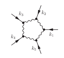
Figure 1: Feynman diagram corresponding to the fifth cumulant where the solid and wiggly lines represent the response and correlation functions

We write Eq. 11 in more compact form where the amputated part of the loop and the external legs are presented distinctly as

$$\langle h^{5}(\mathbf{x},t)\rangle_{c}= \int\frac{d^{d+1}\hat{k}_{1}}{(2\pi)^{d+1}}\int\frac{d^{d+1}\hat{k}_{2}}{(2\pi)^{d+1}}\!\int\frac{d^{d+1}\hat{k}_{3}}{(2\pi)^{d+1}}\int\frac{d^{d+1}\hat{k}_{4}}{(2\pi)^{d+1}}G(\hat{k}_{1})G(\hat{k}_{2})G(\hat{k}_{3})$$ (12)

$$G(\hat{k}_{4})G(-\hat{k}_{1}-\hat{k}_{2}-\hat{k}_{3}-\hat{k}_{4})L(\hat{k}_{1},\hat{k}_{2},\hat{k}_{3},\hat{k}_{4}).$$

where $L$ is the amputated part of the loop diagram (excluding the external legs). The unrenormalised (bare) form of the loop is written as

$$L^{(0)}(\hat{k}_{1},\hat{k}_{2},\hat{k}_{3},\hat{k}_{4})= 32\left(\frac{-\lambda_{0}}{2}\right)^{5}(2D_{0})^{5}\int\frac{d^{d+1}\hat{q_{1}}}{(2\pi)^{d+1}}[\mathbf{q}_{1}\cdot(\mathbf{q}_{1}-\mathbf{k}_{1})][\mathbf{q}_{1}\cdot(\mathbf{q}_{1}+\mathbf{k}_{2})]$$

$$\times[(\mathbf{q}_{1}+\mathbf{k}_{2})\cdot(\mathbf{q}_{1}+\mathbf{k}_{2}+\mathbf{k}_{3})][(\mathbf{q}_{1}+\mathbf{k}_{2}+\mathbf{k}_{3})\cdot(\mathbf{q}_{1}+\mathbf{k}_{2}+\mathbf{k}_{3}+\mathbf{k}_{4})]$$

$$[(\mathbf{q}_{4}-\mathbf{k}_{4})\cdot(\mathbf{k}_{1}+\mathbf{k}_{2}+\mathbf{k}_{3}+\mathbf{k}_{4}+\mathbf{k}_{5})]G_{0}(\hat{q_{1}})G_{0}(\hat{k_{1}}-\hat{q_{1}})$$

$$\times G_{0}(-\hat{q}_{1})G_{0}(\hat{k}_{2}+\hat{q}_{1})G_{0}(-\hat{q}_{1}-\hat{k}_{2})G_{0}(\hat{k}_{3}+\hat{q}_{1}+\hat{k}_{2})G_{0}(-\hat{q}_{1}-\hat{k}_{2}-\hat{k}_{3})$$

$$G_{0}(\hat{k}_{4}+\hat{q}_{1}+\hat{k}_{2}+\hat{k}_{3})G_{0}(-\hat{q}_{1}-\hat{k}_{2}-\hat{k}_{3}-\hat{k}_{4})G_{0}(\hat{q}_{1}+\hat{k}_{5}+\hat{k}_{2}+\hat{k}_{3}+\hat{k}_{4})$$

We shall find a renormalized equivalent of this bare quantity by means of a renormalization scheme employed earlier for the calculation of skewness and kurtosis [41, 42]. We perform the internal frequency integration in Eq. LABEL:L5initial and carry out the integration over the internal momentum restricted in the shell $\Lambda_{0}e^{-r}\leq q\leq\Lambda_{0}$, leading to

$$L^{<}(r)=\frac{35}{8}\frac{\lambda^{5}_{0}D^{5}_{0}}{\pi\nu^{9}_{0}\Lambda^{7}_{0}}\left[\frac{e^{7r}-1}{7}\right].$$ (14)

Considering the iterative nature of the momentum shell elimination in the RG scheme, we obtain the differential equation

$$\frac{dL}{dr}=\frac{35}{8}\frac{\lambda^{5}_{0}D^{5}(r)}{\pi\nu^{9}(r)\Lambda^{7}(r)}.$$ (15)

For large $r$, $\Lambda(r)=\Lambda_{0}e^{-r}$ is identified as the momentum $k$. Substituting the following functional forms

$$\nu(k)=\lambda_{0}\sqrt{\frac{D_{0}}{2\pi\nu_{0}}}k^{-1/2},$$ (16)

and

$$D(k)=\lambda_{0}\sqrt{\frac{D_{0}}{2\pi\nu_{0}}}k^{-1/2},$$ (17)

we integrate the differential equation Eq. 15 and obtain

$$L(r)=\frac{7\pi}{2}\lambda_{0}\frac{D^{3}_{0}}{\nu^{3}_{0}\Lambda^{5}_{0}}e^{5r}.$$ (18)

This expression for the renormalized loop needs to be expressed as a symmetric combination of the external momentum $\hat{k}_{i}$. Consequently $\Lambda_{0}e^{-r}$ is expressed as the fully symmetric combination

$$L(\mathbf{k}_{1},0;\mathbf{k}_{2},0;\mathbf{k}_{3},0;\mathbf{k}_{4},0)=\frac{7\pi}{2}\lambda_{0}\left(\frac{D_{0}}{\nu_{0}}\right)^{3}k^{-5/4}_{1}k^{-5/4}_{2}k^{-5/4}_{3}k^{-5/4}_{4}$$ (19)

for vanishing external frequencies. The frequency dependence is constructed by considering a scaling fuction of the form

$$k_{i}^{5/4}f_{5}\left(\frac{\omega_{i}}{k_{i}^{z}}\right)=\frac{1}{k_{i}^{11/4}\nu^{2}(k_{i})|G(k_{i},\omega_{i})|^{2}}.$$ (20)

This form satisfies the property of real valuedness and it has the desired zero frequency (long time) limit. Consequently, the renormalized loop in Fig. 1 is written as

$$L(\mathbf{k}_{1},\omega_{1};\mathbf{k}_{2},\omega_{2};\mathbf{k}_{3},\omega_{3};\mathbf{k}_{4},\omega_{4})= \frac{7\pi}{2}\lambda_{0}\left(\frac{D_{0}}{\nu_{0}}\right)^{3}k^{11/4}_{1}k^{11/4}_{2}k^{11/4}_{3}k^{11/4}_{4}\nu^{2}(k_{1})\nu^{2}(k_{2})\nu^{2}(k_{3})\nu^{2}(k_{4})$$ (21)

$$|G(k_{1},\omega_{1})|^{2}|G(k_{2},\omega_{2})|^{2}|G(k_{3},\omega_{3})|^{2}|G(k_{4},\omega_{4})|^{2}.$$

Substituting from Eq. 21 in Eq. 12, and carrying out the frequency integrations over $\omega_{1}$, $\omega_{2}$, $\omega_{3}$ and $\omega_{4}$, the fifth cumulant is obtained as

$$\langle h^{5}(\mathbf{x},t)\rangle_{c}= \frac{7}{4}\left(\frac{D_{0}}{2\pi\nu_{0}}\right)^{5/2}\int^{\infty}_{-\infty}dk_{1}\int^{\infty}_{-\infty}dk_{2}\!\int^{\infty}_{-\infty}dk_{3}\!\int^{\infty}_{-\infty}dk_{4}\!$$ (22)

$$J(k_{1},k_{2},k_{3},k_{4})$$

where

$$J(k_{1},k_{2},k_{3},k_{4})=\frac{X(k_{1},k_{2},k_{3},k_{4})}{Y(k_{1},k_{2},k_{3},k_{4})}$$ (23)

with

$$X(k_{1},k_{2},k_{3},k_{4})= (-3|k_{1}|^{6}-3|k_{2}|^{6}-10|k_{2}|^{9/2}(2|k_{3}|^{3/2}+2|k_{4}|^{3/2}+|k_{1}+k_{2}+k_{3}+k_{4}|^{3/2})$$ (24)

$$-10|k_{1}|^{9/2}(2|k_{2}|^{3/2}+2|k_{3}|^{3/2}+2|k_{4}|^{3/2}+|k_{1}+k_{2}+k_{3}+k_{4}|^{3/2})$$

$$-(|k_{3}|^{3/2}+|k_{4}|^{3/2}+|k_{1}+k_{2}+k_{3}+k_{4}|^{3/2})^{2}(3|k_{3}|^{3}+3|k_{4}|^{3}+$$

$$4|k_{4}|^{3/2}|k_{1}+k_{2}+k_{3}+k_{4}|^{3/2}+|k_{1}+k_{2}+k_{3}+k_{4}|^{3}$$

$$+2|k_{3}|^{3/2}(7|k_{4}|^{3/2}+2|k_{1}+k_{2}+k_{3}+k_{4}|^{3/2}))$$

$$-2|k_{2}|^{3}(17|k_{3}|^{3}+17|k_{4}|^{3}+23|k_{4}|^{3/2}|k_{1}+k_{2}+k_{3}+k_{4}|^{3/2}$$

$$+6|k_{1}+k_{2}+k_{3}+k_{4}|^{3}+|k_{3}|^{3/2}(62|k_{4}|^{3/2}+23|k_{1}+k_{2}+k_{3}+k_{4}|^{3/2}))$$

$$-2|k_{1}|^{3}(17|k_{2}|^{3}+17|k_{3}|^{3}+17|k_{4}|^{3}+23|k_{4}|^{3/2}|k_{1}+k_{2}+k_{3}+k_{4}|^{3/2}$$

$$+6|k_{1}+k_{2}+k_{3}+k_{4}|^{3}+|k_{3}|^{3/2}(62|k_{4}|^{3/2}+23|k_{1}+k_{2}+k_{3}+k_{4}|^{3/2})$$

$$+|k_{2}|^{3/2}(62|k_{3}|^{3/2}+62|k_{4}|^{3/2}+23|k_{1}+k_{2}+k_{3}+k_{4}|^{3/2})))$$

and

$$Y(k_{1},k_{2},k_{3},k_{4}) =256|k_{1}|^{5/4}|k_{2}|^{5/4}|k_{3}|^{5/4}|k_{4}|^{5/4}(|k_{1}|^{3/2}+|k-2|^{3/2}+|k_{3}|^{3/2}$$

$$+|k_{4}|^{3/2}+|k_{1}+k_{2}+k_{3}+k_{4}|^{3/2})^{5}$$

Considering the symmetry of the function $J(k_{1},k_{2},k_{3},k_{4})$, the integrations in Eq. 22 can be written as

$$\langle h^{5}(\mathbf{x},t)\rangle_{c}= \frac{7}{4}\left(\frac{D_{0}}{2\pi\nu_{0}}\right)^{5/2}\int^{\infty}_{\mu}dk_{1}\int^{\infty}_{\mu}dk_{2}\!\int^{\infty}_{\mu}dk_{3}\!\int^{\infty}_{\mu}dk_{4}$$ (25)

$$[2J(k_{1},k_{2},k_{3},k_{4})+8J(-k_{1},k_{2},k_{3},k_{4})$$

$$+6J(-k_{1},-k_{2},k_{3},k_{4})].$$

where an infrared cut off $\mu$ has been set due to the infrared divergences in the integrations. We write the integrations as

$$J_{1}(\mu)=\int^{\infty}_{\mu}dk_{1}\int^{\infty}_{\mu}dk_{2}\!\int^{\infty}_{\mu}dk_{3}\!\int^{\infty}_{\mu}dk_{4}J(k_{1},k_{2},k_{3},k_{4}),$$ (26)

$$J_{2}(\mu)=\int^{\infty}_{\mu}dk_{1}\int^{\infty}_{\mu}dk_{2}\!\int^{\infty}_{\mu}dk_{3}\!\int^{\infty}_{\mu}dk_{4}J(-k_{1},k_{2},k_{3},k_{4})$$ (27)

and

$$J_{3}(\mu)=\int^{\infty}_{\mu}dk_{1}\int^{\infty}_{\mu}dk_{2}\!\int^{\infty}_{\mu}dk_{3}\!\int^{\infty}_{\mu}dk_{4}J(-k_{1},-k_{2},k_{3},k_{4})$$ (28)

So that Eq. 25 becomes

$$\langle h^{5}(\mathbf{x},t)\rangle_{c}=\frac{7}{4}\left(\frac{D_{0}}{2\pi\nu_{0}}\right)^{5/2}[2J_{1}(\mu)+8J_{2}(\mu)+6J_{3}(\mu)]$$ (29)

The IR cut off dependent integrals are of the form

$$J_{1}(\mu)=a_{1}\mu^{-5/2}$$

$$J_{2}(\mu)=a_{2}\mu^{-5/2}$$

$$J_{3}(\mu)=a_{3}\mu^{-5/2}$$ (30)

where $a_{1}$, $a_{2}$ and $a_{3}$ are dimensionless constants. Numerical integrations yield the dimensionless constants as

$$a_{1}=\lim_{\mu\rightarrow 0^{+}}[\mu^{5/2}J_{1}(\mu)]=0.00197$$

$$a_{2}=\lim_{\mu\rightarrow 0^{+}}[\mu^{5/2}J_{2}(\mu)]=0.00607$$

$$a_{3}=\lim_{\mu\rightarrow 0^{+}}[\mu^{5/2}J_{3}(\mu)]=0.00583$$ (31)

via numerical convergences. Substituting Eqs. 31, 26, 27, 28, 30 in Eq. 29, we finally obtain the expression for fifth cumulant as

$$\langle h^{5}(\mathbf{x},t)\rangle_{c}=\frac{7}{4}[2a_{1}+8a_{2}+6a_{3}]\left(\frac{D_{0}}{2\pi\nu_{0}}\right)^{5/2}\frac{1}{\mu^{5/2}}$$ (32)

IV Hyperskewness

To calculate the hyperskewness, the expression for the second cumulant is needed. The second cumulant in the frequency and momentum space is expressed as

$$\langle h^{2}(\mathbf{x},t)\rangle_{c}=\langle h^{2}(\mathbf{x},t)\rangle =\int\frac{d^{d}k}{[2\pi]^{d}}\int\frac{d\omega}{[2\pi]}\int\frac{d^{d}k^{\prime}}{(2\pi)^{d}}\int\frac{d\omega^{\prime}}{2\pi}\langle h(\mathbf{k},\omega)h(\mathbf{k}^{\prime},\omega^{\prime})\rangle_{c}$$ (33)

$$e^{i[(\mathbf{k}+\mathbf{k}^{\prime})\cdot\mathbf{x}-(\omega+\omega^{\prime})t]}$$

The Feynman loop corresponding to the correlation function is shown in Fig. 2.

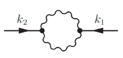
Figure 2: Feynman diagram corresponding to the second cumulant where the solid and wiggly lines represent the response and correlation functions

The frequency and momentum integrations in Eq. 33 can be evaluated [41, 42] and it can be obtained as

$$\langle h^{2}(\mathbf{x},t)\rangle_{c}=\frac{4}{\pi}\left(\frac{D_{0}}{2\pi\nu_{0}}\right)\frac{1}{\mu}$$ (34)

Using Eq.  32 and 34 in 8, we obtain

$$\widetilde{S}=\frac{\langle h^{5}(\mathbf{x},t)\rangle_{c}}{\langle h^{2}(\mathbf{x},t)\rangle_{c}^{5/2}}=\frac{7}{2}\left(\frac{\pi}{4}\right)^{5/2}(a_{1}+4a_{2}+3a_{3})$$ (35)

Substituting the values of $a_{1}$, $a_{2}$ and $a_{3}$ in Eq. 35 we obtain

$$\widetilde{S}=0.0835.$$ (36)

V Discussion and Conclusion

In this paper, we considered the stochastic growth of a surface on a flat geometry (in the stationary state) governed by the $(1+1)$-dimensional KPZ equation. We followed a diagrammatic RG scheme to evaluate the Feynman diagram [Fig. 1] for the fifth cumulant at one loop order corresponding to the $(1+1)$-dimensional KPZ dynamics. We started with the unrenormalized loop with bare parameters ($\nu_{0}$, $\lambda_{0}$ and $D_{0}$ ) and invoked a shell elimination scheme (belonging to the shell $\Lambda_{0}e^{-r}\leq q\leq\Lambda_{0}$) to obtain a differential equation (Eq. 15) representing the recursion relation for successive elimination of momenta in thin shells. The solution of the differential equation yielded the renormalized expression (Eq. 18) for the loop diagram. This facilitated the evaluation of the cumulant $\langle h^{5}(\mathbf{x},t)\rangle_{c}$ given by Eq. 12 involving renormalized quantities. The resulting integrals are found to be infrared divergent and hence $\langle h^{5}(\mathbf{x},t)\rangle_{c}$ depends on the infrared cutoff $\mu$. The momentum integrals are evaluated numerically to obtain $\langle h^{5}(\mathbf{x},t)\rangle_{c}$ as given by Eq. 32. Normalizing this value with respect to the $\langle h^{2}(\mathbf{x},t)\rangle^{5/2}_{c}$ resulted in the hyperskewness value as $\widetilde{S}=0.0835$. It is interesting to note that all parameters of the KPZ dynamics ($\nu_{0}$, $\lambda_{0}$, $D_{0}$) and the momentum cutoffs ($\Lambda_{0}$ and $\mu$) finally cancel out to yield this value, suggesting its universality.

Although there have been many studies on the lower order normalized moments such as skewness and kurtosis, the study of hyperskewness remains a rarity. However, there have been studies based on numerical models that focus on the probability distribution function belonging to the KPZ universality class [29, 34, 36]. In the steady state, this distribution has been shown to be identical with the Baik-Rains distribution [34, 36] with zero mean [43, 29].

The universal Baik-Rains $F_{0}$ distribution is a function of the solutions of Painlevé-II equation, namely, $u^{\prime\prime}(x)=2u^{3}(x)+xu(x)$. Hastings and McLeod [44] obtained a unique solution with the asymptotic boundary conditions $u(x)\sim-Ai(x)$ as $x\rightarrow\infty$ and $u(x)\sim-\sqrt{-x/2}$ as $x\rightarrow-\infty$ where $Ai(x)$ is the Airy function. To solve the Painlevé-II equation, Tracy and Widom performed a numerical integration [45]. Subsequently, Prähofer and Spohn [46] obtained an arbitrary high precession solution by performing Taylor expansions. Baik-Rains distribution is obtained from these solutions via known mathematical relations. On the other hand, the Fredholm determinant representation of the random matrix theory has been observed to be conceptually simpler and numerically efficient than Painlevé-II to obtain the probability distributions [47] ($F_{2}$, $F_{1}$, $F_{0}$, etc.).

It may however be noted that the Baik-Rains value for hyperskewness is $0.3092$ which may be obtained from Fredholm determinant representation[47, 48] as well as from the numerical data [49] via solution of the Painlevé-II. This Baik-Rains value is distinctly higher than our calculated value $\tilde{S}=0.0835$. This underestimation via the RG calculation is due to the fact that the method is based on a perturbative approach where the calculation is carried out only at one-loop order. Since the dynamics is governed by a white noise following a Gaussian distribution, the lowest order approximation appeares to be influenced rather strongly by the Gaussian noise. A similar trend was observed in the one-loop perturbative calculation for kurtosis, namely, $Q=0.1523$ [42] which is lower than the Baik-Rains value $0.2892$. However the value for skewness via the perturbative scheme, namely, $S=0.3237$ [41] is slightly lower than the Baik-Rains value $0.3594$. Thus it appears that the Gaussian white noise plays a more dominant role in the perturbative calculations for the higher order moments, namely, kurtosis and hyperskewness. More involved calculations with the incorporation of higher order contributions in the perturbative expansion are expected to yield better estimates for these higher order moments.

We note that it is next to impossible to obtain a closed-form analytical expression for the full probability distribution starting with the KPZ equation driven by the stochastic noise. Consequently, in an analytical approach, one usually evaluates a few lower and higher order moments (such as skewness, kurtosis and hyperskewness) from the governing dynamics. This outlook has motivated us to evaluate these numbers directly from the $(1+1)$-dimensional KPZ dynamics in the stationary state.

Acknowledgements

T.S. is thankful to the Ministry of Human Resource Development (MHRD), Government of India, for financial support through a scholarship. M.K.N. is indebted to the Indian Institute of Technology Delhi, and particularly to Prof. Senthilkumaran and Prof. Ravishankar, Department of Physics, for hospitality and for extending various facilities at IIT Delhi.

References

References

[1]
Barabási A-L and Stanley H E 1995
Fractal Concepts in Surface Growth(Cambridge: Cambridge University Press)
[2]
Krug J 1997
Adv. Phys.46 139
[3]
Halpin-Healy T and Zhang Y-C 1995
Phys. Rep.254 215
[4]
Family F and Vicsek T 1985
J. Phys. A: Math. Gen.18 L75
[5]
Kardar M, Parisi G, and Zhang Y-C 1986
Phys. Rev. Lett.56 889
[6]
Forster D, Nelson D R, and Stephen M J 1977.
Phys. Rev. A16 732
[7]
Krug J, Meakin P, and Halpin-Healy T 1992
Phys. Rev. A45 638
[8]
Kardar M and Zhang Y-C 1987
Phys. Rev. Lett.58 2087
[9]
Fisher D S and Huse D A 1991
Phys. Rev. B43 10728
[10]
Hwa T and Lässig M 1996
Phys. Rev. Lett.76 2591
[11]
Hwa T 1999
Nature (London)399 17
[12]
Vicsek T, Cserző M, and Horváth V K 1990
Physica A167 315
[13]
Huergo M A C, Pasquale M A, Bolzán A E , Arvia A J, and González P H 2010.
Phys. Rev. E82 031903
[14]
Rubio M A, Edwards C A, Dougherty A, and Gollub J P 1989
Phys. Rev. Lett.63 1685
[15]
Takeuchi K A and Sano M 2010
Phys. Rev. Lett.104 230601
[16]
Takeuchi K A, Sano M, Sasamoto T, and Spohn H 2011
Sci. Rep.1 34
[17]
Myllys M, Maunuksela J, Alava M, Ala-Nissila T, Merikoski J, and
Timonen J 2001
Phys. Rev. E64 036101
[18]
Miettinena L, Myllys M, Merikoski J, and Timonen J 2005
Eur. Phys. J. B46 55
[19]
Meakin P, Ramanlal P, Sander L M, and Ball R C 1986
Phys. Rev. A34 5091
[20]
Eden M 1961
(University of California Press, Berkeley).
[21]
Plischke M and Rácz Z 1984
Phys. Rev. Lett.53 415
[22]
Jullien R and Botet R 1985
Phys. Rev. Lett.54 2055
[23]
Plischke M and Rácz Z 1985
Phys. Rev. A32 3825
[24]
Meakin P 1993
Phys. Rep.235 189
[25]
Plischke M, Rácz Z, and Liu D 1987
Phys. Rev. B35 3485
[26]
W. van Saarloos and G H. Gilmer 1986
Phys. Rev. B33 4927
[27]
Goldenfeld N 1984
J. Phys. A17 2807
[28]
Krug J and Spohn H 1988
Phys. Rev. A38 4271
[29]
Prähofer M and Spohn H 2000.
Phys. Rev. Lett.84 4882
[30]
Baik J and Rains E M 2001
Random Matrix Models and Their Applications.
edited by Bleher P M and A. R. Its (Cambridge: Cambridge University Press).
[31]
Sasamoto T and Spohn H 2010
Phys. Rev. Lett.104 230602
[32]
Sasamoto T and Spohn H 2010
J. Stat. Mech: Theory and Exp.11 13
[33]
Calabrese P and Le Doussal P 2011
Phys. Rev. Lett.106 250603
[34]
Takeuchi K A 2013
Phys. Rev. Lett.110 210604,
[35]
Imamura T and Sasamoto T 2012
Phys. Rev. Lett.108 190603
[36]
Halpin-Healy T and Lin Y 2014
Phys. Rev. E89 010103
[37]
Halpin-Healy T and Takeuchi K A 2015
J. Stat. Phys.160, 794
[38]
Shim Y and Landau D P 2001
Phys. Rev. E64 036110
[39]
Huse D A, Henley C L, and Fisher D S 1985
Phys. Rev. Lett.55 2924
[40]
Parisi G 1990
J. Phys. France51 1595
[41]
Singha T and Nandy M K 2014
Phys. Rev. E90 062402
[42]
Singha T and Nandy M K 2015
J. Stat. Mech.: Theory and Exp.P05020
[43]
Baik J and Rains E M 2000
J.Stat. Phys.100 523,
[44]
Hastings S P and McLeod J B 1980
Archive for Rational Mechanics and Analysis73, 1,
[45]
Tracy C A and Widom H 1994
Commun. Math. Phys.159 151
[46]
Prähofer M and Spohn H 2004
J. Stat. Phys.115, 1
[47]
Bornemann F
http://arxiv.org/abs/0904.1581
[48]
Bornemann F (2015)
private communication
[49]
Prähofer M and Spohn H
http://www-m5.ma.tum.de/KPZ