Abstract

We derive the exact spectra as well as partition functions for a class of $BC_{N}$ type of spin Calogero models, whose Hamiltonians are constructed by using supersymmetric analogues of polarized spin reversal operators (SAPSRO). The strong coupling limit of these spin Calogero models yields $BC_{N}$ type of Polychronakos-Frahm (PF) spin chains with SAPSRO. By applying the freezing trick, we obtain an exact expression for the partition functions of such PF spin chains. We also derive a formula which expresses the partition function of any $BC_{N}$ type of PF spin chain with SAPSRO in terms of partition functions of several $A_{K}$ type of supersymmetric PF spin chains, where $K\leqslant N-1$. Subsequently we show that an extended boson-fermion duality relation is obeyed by the partition functions of the $BC_{N}$ type of PF chains with SAPSRO. Some spectral properties of these spin chains, like level density distribution and nearest neighbour spacing distribution, are also studied.

PACS No. : 02.30.Ik, 05.30.-d, 75.10.Pq, 75.10.Jm

Keywords: Exactly solvable quantum spin models, Polarized spin reversal operator, Boson-fermion duality relation, Yangian quantum group, Supersymmetry

1 Introduction

Remarkable progress has been made in recent years in the computation of exact spectra, partition functions and correlation functions of one-dimensional quantum integrable spin chains with long-range interactions as well as their supersymmetric generalizations [1, 2, 3, 4, 5, 6, 7, 8, 9, 10, 11, 12, 13, 14, 15, 16, 17, 18, 19, 20, 21, 22, 23, 24]. Exact solutions of this type of quantum spin chains with periodic and open boundary conditions have been found to be closely connected with diverse areas of physics and mathematics like condensed matter systems exhibiting generalized exclusion statistics [5, 23, 24, 25], quantum Hall effect [26], quantum electric transport phenomena [27, 28], calculation of higher loop effects in the spectra of trace operators of planar ${\mathcal{N}}=4$ super Yang–Mills theory [29, 30, 31], Dunkl operators related to various root systems  [32, 33], random matrix theory [34], and Yangian quantum groups [4, 5, 9, 17, 35, 36, 37]. Furthermore, it has been recently observed that exactly solvable spin chains with long-range interactions can be generated through some lattice discretizations of conformal field theories related to the ‘infinite matrix product states’ [38, 39, 40, 41].

The study of quantum integrable spin chains with long-range interactions was pioneered by Haldane and Shastry, who derived the exact spectrum of a spin-$\frac{1}{2}~{}$chain with lattice sites equally spaced on a circle and spins interacting through pairwise exchange interactions inversely proportional to the square of their chord distances [1, 2]. It has been found that, the exact ground state wave function of this su($2$) symmetric Haldane-Shastry (HS) spin chain coincides with the $U\to\infty$ limit of Gutzwiller’s variational wave function describing the ground state of the one-dimensional Hubbard model [42, 43, 44]. A close relation between the su($m$) generalizations of this HS spin chain and the (trigonometric) Sutherland model has been established by using the ‘freezing trick’ [6, 45], which we briefly describe in the following. In contrast to the case of HS spin chain where lattice sites are fixed at equidistant positions on a circle, the particles of the su($m$) spin Sutherland model can move on a circle and they contain both coordinate as well as spin degrees of freedom. However, in the strong coupling limit, the coordinates of these particles decouple from their spins and ‘freeze’ at the minimum value of the scalar part of the potential. Furthermore, this minimum value of the scalar part of the potential yields the equally spaced lattice points of the HS spin chain. As a result, in the strong coupling limit, the dynamics of the decoupled spin degrees of freedom of the su($m$) spin Sutherland model is governed by the Hamiltonian of the su($m$) HS model. Application of this freezing trick to the su($m$) spin (rational) Calogero model leads to another quantum integrable spin chain with long-range interaction [6], which is known in the literature as the su($m$) Polychronakos or Polychronakos–Frahm (PF) spin chain. The sites of such rational PF spin chain are inhomogeneously spaced on a line and, in fact, they coincide with the zeros of the Hermite polynomial [7]. Indeed, the Hamiltonian of the su($m$) PF spin chain is given by

$$\mathcal{H}_{\mathrm{PF}}^{(m)}=\sum_{1\leqslant i<j\leqslant N}\frac{1-\epsilon P_{ij}^{(m)}}{(\rho_{i}-\rho_{j})^{2}}\,,$$ (1.1)

where $\epsilon=1~{}(-1)$ corresponds to the ferromagnetic (anti-ferromagnetic) case, $P_{ij}^{(m)}$ denotes the exchange operator which interchanges the ‘spins’ (taking $m$ possible values) of $i$-th and $j$-th lattice sites and $\rho_{i}$ denotes the $i$-th zero of the Hermite polynomial of degree $N$. Due to the decoupling of the spin and coordinate degrees of freedom of the su($m$) spin Calogero model for large values of its coupling constant, an exact expression for the partition function of su($m$) PF spin chain can be derived by dividing the partition function of the su($m$) spin Calogero model through that of the spinless Calogero model [8]. Similarly, the partition function of su($m$) HS spin chain can be computed by dividing the partition function of the su($m$) spin Sutherland model through that of the spinless Sutherland model [12].

As is well known, supersymmetric spin chains with different type of interactions play an important role in describing some quantum impurity problems and disordered systems in condensed matter physics, where holes moving in the dynamical background of spins behave as bosons, and spin-1/2 electrons behave as fermions [46, 47, 48, 49, 50]. The above mentioned PF and HS spin chains admit natural su($m|n$) supersymmetric generalizations, where each lattice site has $m$ number of bosonic and $n$ number of fermionic degrees of freedom. Exact expressions for the partition functions of such su($m|n$) PF and HS spin chains can also be computed by using the method of freezing trick [10, 11, 13]. It is found that these partition functions satisfy remarkable duality relations under the exchange of bosonic and fermionic degrees of freedom.

It may be noted that, the strength of interaction between any two spins in the Hamiltonian (1.1) depends only on the difference of their site coordinates. This type of translationally invariant Hamiltonians of quantum integrable spin chains (and their supersymmetric generalizations) are closely related to the $A_{N-1}$ type of root system. Indeed, the spin-spin interactions appearing in such Hamiltonians are given by the permutation operators which yield a realization of the $A_{N-1}$ type of Weyl group. However, it is also possible to construct exactly solvable variants of HS and PF spin chains associated with the $BC_{N}$, $B_{N}$, $C_{N}$ and $D_{N}$ root systems [18, 19, 20, 21, 22, 51, 52, 53]. A key feature of such spin chains is the presence of boundary points with reflecting mirrors, due to which the spins not only interact with each other but also with their mirror images. As a result, the corresponding Hamiltonians break the translational invariance. It may also be noted that, Hamiltonians of the spin chains associated with the $BC_{N}$ root system and its $B_{N}$, $C_{N}$ and $D_{N}$ degenerations contain reflection operators like $S_{i}$ ($i=1,\dots,N$), which satisfy the relation $S_{i}^{2}=1\hskip-2.84526pt{\rm l}$ and few other relations associated with the corresponding Weyl algebra. Representing such $S_{i}$ as the spin reversal operator $P_{i}$ which changes the sign of the spin component on the $i$-th lattice site, the partition functions of HS and PF spin chains associated with the $BC_{N}$, $B_{N}$, $C_{N}$ and $D_{N}$ root systems have been computed by using the freezing trick [21, 22, 51, 52, 53]. Furthermore, by taking $S_{i}$ as the spin reversal operator on a superspace, the partition function of a supersymmetric analogue of the PF spin chain associated with $BC_{N}$ root system has also been computed in a similar way [54].

However it is worth noting that, the above mentioned representations of reflection operators as the spin reversal operators is by no means the only possible choice. Indeed, by choosing all reflection operators as the trivial identity operator, it has been found that [19] a spin-$\frac{1}{2}~{}$HS chain associated with the $BC_{N}$ root system leads to an integrable su($2$) invariant spin model which was first studied by Simons and Altshuler [18]. Furthermore, a class of exactly solvable spin Calogero models of $BC_{N}$ type and the corresponding PF chains have been introduced recently [55], where the reflection operators are represented by arbitrarily polarized spin reversal operators (PSRO) $P_{i}^{(m_{1},m_{2})}$, which act as the identity on the first $m_{1}$ elements of the spin basis on the $i$-th lattice site and as minus the identity on the rest of the spin basis. Consequently, depending on the action of $P_{i}^{(m_{1},m_{2})}$, the basis vectors of the $m$-dimensional spin space on each lattice site can be grouped into two cases — $m_{1}$ elements with positive parity and $m_{2}$ elements with negative parity. Using a similarity transformation, it can be shown that the PSRO reduce to the usual spin reversal operators $P_{i}$ (up to a sign factor) when $m_{1}=m_{2}$ or $m_{1}=m_{2}\pm 1$. For the remaining values of the discrete parameters $m_{1}$ and $m_{2}$, the systems constructed in the later reference differ from the standard Calogero and PF models of $BC_{N}$-type. In particular, for the case $m_{2}=0$ and $m_{1}=m$, $P_{i}$ reduces to the identity operator and leads to a novel su($m$) invariant spin chain, which is described by the Hamiltonian

$${\mathcal{H}}^{(m,0)}=\sum_{1\leqslant i\neq j\leqslant N}\frac{y_{i}+y_{j}}{(y_{i}-y_{j})^{2}}\,(1-\epsilon P_{ij}^{(m)})\,,$$ (1.2)

where $\epsilon=\pm 1$, $y_{i}$ denotes the $i$-th zero of the generalized Laguerre polynomial $L_{N}^{\beta-1}$. Thus, the lattice sites of ${\mathcal{H}}^{(m,0)}$ implicitly depend on the real positive parameter $\beta$. Computing the partition function of the spin chain (1.2) by using the freezing trick and analyzing such partition function, it has been found that the spectrum of this spin chain coincides (up to a scale factor) with that of the original PF model (1.1) [55]. However, a deeper reason for this surprising coincidence has not been fully understood till now.

Even though the spectrum and partition function of the supersymmetric generalization of the $A_{N-1}$ type of PF spin chain (1.1) have been computed earlier [10, 11], no such result is available till now for the supersymmetric generalization of the spin chain (1.2). In this context it is interesting to ask whether it is possible to compute the partition function for the supersymmetric version of the spin chain (1.2) by using the freezing trick, and whether the corresponding spectrum can be related in a simple way with that of the supersymmetric PF spin chain. In the present article we try to answer these questions by constructing supersymmetric analogues of PSRO (SAPSRO), which would satisfy the $BC_{N}$ type of Weyl algebra. By using such SAPSRO, we obtain a rather large class of exactly solvable spin Calogero models and PF chains of $BC_{N}$ type. In a particular case where polarization is minimal, SAPSRO reduce to the supersymmetric analogues of usual spin reversal operators and lead to the spin Calogero models as well as PF chains of $BC_{N}$ type which have been studied earlier [54]. However, in all other cases, these SAPSRO can be used to generate novel exactly solvable spin Calogero models and PF chains of $BC_{N}$ type. In particular, for the case where polarization is maximal, we find that SAPSRO reduces to the trivial identity operator and lead to a supersymmetric extension of the spin chain (1.2), whose partition function and spectrum can be computed by using the freezing trick.

Another interesting topic which we shall address in this paper is a modification of the usual boson-fermion duality relation which is satisfied by the partition functions of $A_{N-1}$ type of spin chains. This type of modified duality relation has been studied earlier for the special case of $BC_{N}$ type of PF chains associated with the supersymmetric analogue of the spin reversal operators [54]. It has been observed that this duality relation not only involves the exchange of bosonic and fermionic degrees freedom, but also certain changes of the two discrete parameters which appear in the corresponding Hamiltonian. However, the full significance for such change of the two discrete parameters has not been explored till now. We find that the underlying reason for such change of the discrete parameters can be understood in a natural way if one studies the duality relation for $BC_{N}$ type of PF chains in the broader context of SAPSRO. Indeed, in this paper we consider a new quantum number which measures the parity of the spin states under the action of SAPSRO. Curiously, it turns out that the partition functions of the spin chains now satisfy an ‘extended’ boson-fermion duality relation, which involves not only the exchange of bosonic and fermionic degrees of freedom, but also the exchange of positive and negative parity degrees of freedom associated with the SAPSRO.

The arrangement of this paper is as follows. In Section 2, we construct SAPSRO which, along with the supersymmetric spin exchange operators, lead to new representations of the $BC_{N}$ type of Weyl algebra and related PF spin chains with open boundary conditions. Next, in Section 3, we consider $BC_{N}$ type of spin Calogero models associated with SAPSRO, which in the strong coupling limit yield the above mentioned class of PF spin chains. We derive the exact spectra as well as partition functions of these $BC_{N}$ type of spin Calogero models with SAPSRO. By applying the freezing trick, subsequently we obtain an exact expression for the partition functions of the related PF spin chains. In Section 4, we derive a formula which expresses the partition function of any $BC_{N}$ type of PF spin chain with SAPSRO in terms of partition functions of several $A_{K}$ type of supersymmetric PF spin chains, where $K\leqslant N-1$. By taking a particular limit of the above mentioned formula, we find that the partition function of the supersymmetric extension of the spin chain (1.2) coincides with that of a $A_{N-1}$ type of supersymmetric PF spin chain. In Section 5, we derive an extended boson-fermion duality relation for the $BC_{N}$ type of PF chains with SAPSRO. In Section 6, we compute the ground state and the highest state energies of these spin chains. Some spectral properties of these spin chains, like level density distribution and nearest neighbour spacing distribution, are studied in Section 7. Section 8 is the concluding section.

2 $BC_{N}$ type of Weyl algebra and related PF chains

As is well known, different representations of the $BC_{N}$ type of Weyl algebra play a key role in constructing exactly solvable variants of HS and PF spin chains with open boundary conditions. This $BC_{N}$ type of Weyl algebra is generated by the elements $\mathcal{W}_{ij}$ and $\mathcal{W}_{i}\,$ satisfying the relations

$$\mathcal{W}_{ij}^{2}=1\hskip-2.84526pt{\rm l}\,,~{}~{}~{}~{}\mathcal{W}_{ij}\mathcal{W}_{jk}=\mathcal{W}_{ik}\mathcal{W}_{ij}=\mathcal{W}_{jk}\mathcal{W}_{ik}\,,~{}~{}~{}~{}\mathcal{W}_{ij}\mathcal{W}_{kl}=\mathcal{W}_{kl}\mathcal{W}_{ij}\,,$$ (2.1a)

$$\mathcal{W}_{i}^{2}=1\hskip-2.84526pt{\rm l}\,,~{}~{}~{}~{}\mathcal{W}_{i}\mathcal{W}_{j}=\mathcal{W}_{j}\mathcal{W}_{i}\,,~{}~{}~{}~{}\mathcal{W}_{ij}\mathcal{W}_{k}=\mathcal{W}_{k}\mathcal{W}_{ij}\,,~{}~{}~{}~{}\mathcal{W}_{ij}\mathcal{W}_{j}=\mathcal{W}_{i}\mathcal{W}_{ij}\,,$$ (2.1b)

where $i,~{}j,~{}k,~{}l$ are all different indices. Let us assume that the Hermitian operators $\mathcal{P}_{ij}$ and $\mathcal{P}_{i}\,$ yield a realization of the elements $\mathcal{W}_{ij}$ and $\mathcal{W}_{i}\,$ respectively on an appropriate spin space. Motivated by the earlier works [20, 22, 54, 55], we define a general form of Hamiltonian for the $BC_{N}$ type of PF spin chain as

$$\mathcal{H}=\sum_{i\neq j}\left[\frac{1-\mathcal{P}_{ij}}{(\xi_{i}-\xi_{j})^{2}}+\frac{1-\widetilde{\mathcal{P}}_{ij}}{(\xi_{i}+\xi_{j})^{2}}\right]+\beta\sum_{i=1}^{N}\frac{1-\mathcal{P}_{i}}{\xi_{i}^{2}}\,,$$ (2.2)

where $\beta$ is a positive parameter, $\widetilde{\mathcal{P}}_{ij}=\mathcal{P}_{i}\mathcal{P}_{j}\mathcal{P}_{ij}$, $\xi_{i}=\sqrt{2y_{i}}$ and $y_{i}$ represents the $i$-th zero point of the generalized Laguerre polynomial $L_{N}^{\beta-1}$. In the following, at first we shall briefly discuss how this general form of Hamiltonian yields already known PF spin chains associated with the $BC_{N}$ root system for different choices of the operators $\mathcal{P}_{ij}$ and $\mathcal{P}_{i}$. Subsequently, we shall construct SAPSRO which, along with the supersymmetric spin exchange operators, would lead to a new class of representations for the $BC_{N}$ type of Weyl algebra and the related PF chains.

In the case of a non-supersymmetric spin chain with $N$ number of lattice sites, the total internal space $\boldsymbol{\Sigma}^{(m)}$ is expressed as

$$\boldsymbol{\Sigma}^{(m)}\equiv\underbrace{\mathcal{C}_{m}\otimes\mathcal{C}_{m}\otimes\cdots\otimes\mathcal{C}_{m}}_{N}\,,$$ (2.3)

where $\mathcal{C}_{m}$ denotes a $m$-dimensional complex vector space. In terms of orthonormal basis vectors, $\boldsymbol{\Sigma}^{(m)}$ may be written as

$$\boldsymbol{\Sigma}^{(m)}=\Big{\langle}|s_{1},\cdots,s_{N}\rangle~{}\Big{|}s_{i}\in\{-M,-M+1,\cdots,M\};~{}M=\frac{m-1}{2}\Big{\rangle}\,.$$ (2.4)

The spin exchange operator $P_{ij}^{(m)}$ and the spin reversal operator $P_{i}$ act on these orthonormal basis vectors as

$$P_{ij}^{(m)}|s_{1}\,,\cdots,s_{i}\,,\cdots,s_{j}\,,\cdots,s_{N}\rangle=|s_{1}\,,\cdots,s_{j}\,,\cdots,s_{i}\,,\cdots,s_{N}\rangle\,,$$ (2.5a)

$$P_{i}|s_{1}\,,\cdots,s_{i}\,,\cdots,s_{N}\rangle=|s_{1}\,,\cdots,-s_{i}\,,\cdots,s_{N}\rangle\,.$$ (2.5b)

It is easy to check that $\epsilon P_{ij}^{(m)}$ and $\epsilon^{\prime}P_{i}$ (where $\epsilon,\epsilon^{\prime}=\pm 1$ are two independent signs) yield a realization of the $BC_{N}$ type of Weyl algebra (2.1). Substituting $\epsilon P_{ij}^{(m)}$ and $\epsilon^{\prime}P_{i}$ in the places of $\mathcal{P}_{ij}$ and $\mathcal{P}_{i}$ respectively in the general form of Hamiltonian (2.2), one obtains an exactly solvable $BC_{N}$ type of non-supersymmetric PF spin chain whose partition function has been computed by using the freezing trick [22].

For the purpose of generalizing the above mentioned spin chain through PSRO, it is convenient to define the space $\boldsymbol{\Sigma}^{(m)}$ through a different set of orthonormal basis vectors as

$$\boldsymbol{\Sigma}^{(m)}=\Big{\langle}|s_{1},\cdots,s_{N}\rangle~{}\Big{|}s_{i}\in\{1,2,\cdots,m\}\Big{\rangle}\,.$$ (2.6)

The action of spin exchange operator $P_{ij}^{(m)}$ on these orthonormal basis vectors is again given by an equation of the form (2.5a). However, the spin reversal operator is replaced by PSRO (denoted by $P_{i}^{(m_{1},m_{2})}$ for the $i$-th lattice site) which acts on these orthonormal basis vectors as [55]

$$P_{i}^{(m_{1},m_{2})}|s_{1},\cdots,s_{i},\cdots,s_{N}\rangle=(-1)^{f(s_{i})}|s_{1},\cdots,s_{i},\cdots,s_{N}\rangle,$$ (2.7)

where

$$f(s_{i})=\left\{\begin{array}[]{ll}0,&\mbox{~{}if $s_{i}\in\{1,2,\cdots,m_{1}\}$, }\\ 1,&\mbox{~{}if $s_{i}\in\{m_{1}+1,\cdots,m_{1}+m_{2}\}$, }\end{array}\right.$$

and $m_{1}$ and $m_{2}$ are two arbitrary non-negative integers satisfying the relation $m_{1}+m_{2}=m$. Using Eqs. (2.5a) and (2.7), it is easy to check that $\epsilon P_{ij}^{(m)}$ and $P_{i}^{(m_{1},m_{2})}$ yield a realization of $BC_{N}$ type of Weyl algebra (2.1). Substituting $\epsilon P_{ij}^{(m)}$ and $P_{i}^{(m_{1},m_{2})}$ (in places of $\mathcal{P}_{ij}$ and $\mathcal{P}_{i}$, respectively) in the general form of Hamiltonian (2.2) and taking different possible values of $m_{1}$ and $m_{2}$, one obtains a class of exactly solvable $BC_{N}$ type of PF spin chains with PSRO [55]. Using a similarity transform it has been shown in the latter reference that, in the special case given by $m_{1}=m_{2}$ ($m_{1}=m_{2}+\epsilon^{\prime}$) for even (odd) values of $m$, the operator $P_{i}^{(m_{1},m_{2})}$ becomes equivalent to $\epsilon^{\prime}{P}_{i}$. Consequently, PF spin chain associated with PSRO reduces to PF spin chain associated with spin reversal operators in this special case. It may also be observed that, in another special case given by $m_{1}=m,~{}m_{2}=0$, $P_{i}^{(m_{1},m_{2})}$ in (2.7) reduces to the trivial identity operator and the corresponding Hamiltonian (2.2) yields the exactly solvable $su(m)$ invariant spin chain (1.2) which has been discussed earlier.

Next, for the purpose of discussing representations of the $BC_{N}$ type of Weyl algebra (2.1) on a superspace, we consider a set of operators like $C_{j\alpha}^{\dagger}$($C_{j\alpha}$) which creates (annihilates) a particle of species $\alpha$ on the $j$-th lattice site. The parity of these operators are defined as

$$\pi(C_{j\alpha})=\pi(C_{j\alpha}^{\dagger})=0~{}\mathrm{for}~{}\alpha\in[1,2,....,m]\,,$$

$$\pi(C_{j\alpha})=\pi(C_{j\alpha}^{\dagger})=1~{}\mathrm{for}~{}\alpha\in[m+1,m+2,....,m+n]\,,$$

i.e, they are assumed to be bosonic when $\alpha\in[1,2,....,m]$ and fermionic when $\alpha\in[m+1,m+2,....,m+n]$. These operators satisfy commutation (anti-commutation) relations given by

$$[C_{j\alpha},C_{k\beta}]_{\pm}=0\,,~{}[C_{j\alpha}^{\dagger},C_{k\beta}^{\dagger}]_{\pm}=0\,,~{}[C_{j\alpha},C_{k\beta}^{\dagger}]_{\pm}=\delta_{jk}\delta_{\alpha\beta}\,,$$ (2.8)

where $[C,D]_{\pm}\equiv CD-(-1)^{\pi(C)\pi(D)}DC$. On a subspace of the corresponding Fock space, where each lattice site is occupied by only one particle (i.e., $\sum_{\alpha=1}^{m+n}C_{j\alpha}^{\dagger}C_{j\alpha}=1$ for all $j$), the supersymmetric exchange operator is defined as

$$\hat{P}_{ij}^{(m|n)}\equiv\sum_{\alpha,\beta=1}^{m+n}C_{i\alpha}^{\dagger}C_{j\beta}^{\dagger}C_{i\beta}C_{j\alpha}\,.$$ (2.9)

This supersymmetric exchange operator can equivalently be described as an operator on a spin space in the following way. Let us assume that each lattice site of a spin chain is occupied by either one of the $m$ number of ‘bosonic’ spins or one of the $n$ number of ‘fermionic’ spins. Hence, the total internal space associated with such spin chain can be expressed as

$$\boldsymbol{\Sigma}^{(m|n)}\equiv\underbrace{\mathcal{C}_{m+n}\otimes\mathcal{C}_{m+n}\otimes\cdots\otimes\mathcal{C}_{m+n}}_{N}\,.$$ (2.10)

Using the notation of Ref. [54], the orthonormal basis vectors of $\boldsymbol{\Sigma}^{(m|n)}$ may be denoted as $|s_{1},\cdots,s_{N}\rangle$, where $s_{i}\equiv(s_{i}^{1},s_{i}^{2})$ is a vector with two components taking values within the range

$$s_{i}^{1}\equiv\pi(s_{i})=\left\{\begin{array}[]{ll}0,&\mbox{~{}for bosons, }\\ 1,&\mbox{~{}for fermions, }\end{array}\right.$$ (2.11c)

$$s_{i}^{2}\in\left\{\hskip-11.38092pt\begin{array}[]{ll}&\mbox{~{} $\{-\frac{m-1}{2},-\frac{m-1}{2}+1,\cdots,\frac{m-1}{2}\},~{}~{}\mathrm{if}~{}\pi(s_{i})=0$, }\\ &~{}\mbox{~{}$\{-\frac{n-1}{2},-\frac{n-1}{2}+1,\cdots,\frac{n-1}{2}\},~{}~{}\mathrm{if}~{}\pi(s_{i})=1$. }\end{array}\right.$$ (2.11f)

Thus the component $s_{i}^{1}\equiv\pi(s_{i})$ denotes the type of spin (bosonic or fermionic) and the component $s_{i}^{2}$ denotes the numerical value of the spin. A supersymmetric spin exchange operator $P_{ij}^{(m|n)}$ has been defined earlier on the space $\boldsymbol{\Sigma}^{(m|n)}$ as [13, 35]

$$P_{ij}^{(m|n)}|s_{1},\cdots,s_{i},\cdots,s_{j},\cdots,s_{N}\rangle=(-1)^{\alpha_{ij}(\mathbf{s})}|s_{1},\cdots,s_{j},\cdots,s_{i},\cdots,s_{N}\rangle,$$ (2.12)

where $\alpha_{ij}(\mathbf{s})=\pi(s_{i})\pi(s_{j})+\left(\pi(s_{i})+\pi(s_{j})\right)\,h_{ij}(\mathbf{s})$ and $h_{ij}(\mathbf{s})=\sum_{k=i+1}^{j-1}\pi(s_{k})$ denotes the number of fermions in between the $i$-th and $j$-th spins. From Eq. (2.12) it follows that, the exchange of two bosonic (fermionic) spins produces a phase factor of $1(-1)$. However, the exchange one bosonic spin with one fermionic spin (or, vice versa) produces a phase factor of $(-1)^{h_{ij}(\mathbf{s})}$. Using the commutation (anti-commutation) relations in (2.8), it can be shown that $\hat{P}_{ij}^{(m|n)}$ in (2.9) is completely equivalent to $P_{ij}^{(m|n)}$ in (2.12) [13, 35].

A supersymmetric analogue of the spin reversal operator $P_{i}$ (2.5b) can also be defined on the space $\boldsymbol{\Sigma}^{(m|n)}$ [54]. While acting on the basis vectors of $\boldsymbol{\Sigma}^{(m|n)}$, this supersymmetric analogue of spin reversal operator (denoted by $P_{i}^{\epsilon\epsilon^{\prime}}$) reverses the value of the $i$-th spin without affecting its type and multiplies the state by a sign factor. More precisely, the action of $P_{i}^{\epsilon\epsilon^{\prime}}$ is given by

$$P_{i}^{\epsilon\epsilon^{\prime}}|s_{1},\cdots,s_{i},\cdots,s_{N}\rangle=\rho(s_{i})|s_{1},\cdots,s_{i}^{-},\cdots,s_{N}\rangle,$$ (2.13)

where $s_{i}^{-}=(s_{i}^{1},-s_{i}^{2})$, $\rho(s_{i})=\epsilon~{}(\epsilon^{\prime})$ for $\pi(s_{i})=0~{}(1)$, and $\epsilon,\epsilon^{\prime}=\pm 1$ are two independent signs. With the help of (2.12) and (2.13), one can easily check that $P_{ij}^{(m|n)}$ and $P_{i}^{\epsilon\epsilon^{\prime}}$ yield a realization of the $BC_{N}$ type of Weyl algebra (2.1). Substitution of $P_{ij}^{(m|n)}$ and $P_{i}^{\epsilon\epsilon^{\prime}}$ in Eq. (2.2) yields an exactly solvable Hamiltonian given by [54]

$$\mathcal{H}^{(m|n)}_{\epsilon\epsilon^{\prime}}=\sum_{i\neq j}\left[\frac{1-P_{ij}^{(m|n)}}{(\xi_{i}-\xi_{j})^{2}}+\frac{1-\widetilde{P}_{ij}^{(m|n)}}{(\xi_{i}+\xi_{j})^{2}}\right]+\beta\sum_{i=1}^{N}\frac{1-P_{i}^{\epsilon\epsilon^{\prime}}}{\xi_{i}^{2}}\,,$$ (2.14)

where $\widetilde{P}_{ij}^{(m|n)}=P_{i}^{\epsilon\epsilon^{\prime}}P_{j}^{\epsilon\epsilon^{\prime}}P_{ij}^{(m|n)}$. However, since $\mathcal{H}^{(m|n)}_{\epsilon\epsilon^{\prime}}$ in the above equation does not reduce to ${\mathcal{H}}^{(m,0)}$ in (1.2) for the special case $n=0$ (and for any possible choice of $\epsilon$ and $\epsilon^{\prime}$), the former Hamiltonian can not be considered as a supersymmetric extension of the later one.

At present our aim is to construct SAPSRO which would satisfy the $BC_{N}$ type of Weyl algebra (2.1). To this end, we denote the total internal space of the related spin system as $\boldsymbol{\Sigma}^{(m_{1},m_{2}|n_{1},n_{2})}$, where $m_{1},~{}m_{2},~{}n_{1},~{}n_{2}$ are some arbitrary non-negative integers satisfying the relations $m_{1}+m_{2}=m$ and $n_{1}+n_{2}=n$. This $\boldsymbol{\Sigma}^{(m_{1},m_{2}|n_{1},n_{2})}$ can be expressed in a direct product form exactly like (2.10), but each $s_{i}$ within the corresponding basis vectors now possess an extra quantum number associated with the action of SAPSRO. More precisely, $\boldsymbol{\Sigma}^{(m_{1},m_{2}|n_{1},n_{2})}$ is spanned by orthonormal state vectors like $|s_{1},\cdots,s_{N}\rangle$, where $s_{i}\equiv(s_{i}^{1},s_{i}^{2},s_{i}^{3})$ is a vector with three components taking values within the range

$$s_{i}^{1}\equiv\pi(s_{i})=\left\{\begin{array}[]{ll}0,&\mbox{~{}for bosons, }\\ 1,&\mbox{~{}for fermions, }\end{array}\right.$$ (2.15c)

$$s_{i}^{2}\equiv f(s_{i})=\left\{\begin{array}[]{ll}0,&\mbox{~{}for positive parity under SAPSRO}\\ 1,&\mbox{~{}for negative parity under SAPSRO, }\end{array}\right.$$ (2.15f)

$$s_{i}^{3}\in\left\{\hskip-13.37282pt\begin{array}[]{llll}&\mbox{~{} $\{1,2,\cdots,m_{1}\},~{}\mathrm{if}~{}\pi(s_{i})=0~{}\mathrm{and}~{}f(s_{i})=0$, }\\ &~{}\mbox{~{}$\{1,2,\cdots,m_{2}\},~{}\mathrm{if}~{}\pi(s_{i})=0~{}\mathrm{and}~{}f(s_{i})=1$, }\\ &~{}\mbox{~{}$\{1,2,\cdots,n_{1}\},~{}\mathrm{if}~{}\pi(s_{i})=1~{}\mathrm{and}~{}f(s_{i})=0$, }\\ &~{}\mbox{~{}$\{1,2,\cdots,n_{2}\},~{}\mathrm{if}~{}\pi(s_{i})=1~{}\mathrm{and}~{}f(s_{i})=1$. }\end{array}\right.$$ (2.15k)

Indeed, we define the action of SAPSRO (denoted by $P_{i}^{(m_{1},m_{2}|n_{1},n_{2})}$) on these state vectors as

$$P_{i}^{(m_{1},m_{2}|n_{1},n_{2})}|s_{1},\cdots,s_{i},\cdots,s_{N}\rangle=(-1)^{f(s_{i})}|s_{1},\cdots,s_{i},\cdots,s_{N}\rangle,$$ (2.16)

which shows that $s_{i}^{2}\equiv f(s_{i})$ is determined through the parity of the spin $s_{i}$ under the action of SAPSRO. As before, the action of supersymmetric spin exchange operator $P_{ij}^{(m|n)}$ on the space $\boldsymbol{\Sigma}^{(m_{1},m_{2}|n_{1},n_{2})}$ is given by an equation of the form (2.12), where the phase factor $\alpha_{ij}(\mathbf{s})$ depends on the first components of the spins like $s_{k}^{1}\equiv\pi(s_{k})$. Using Eqs. (2.12) and (2.16), we find that $P_{ij}^{(m|n)}$ and $P_{i}^{(m_{1},m_{2}|n_{1},n_{2})}$ yield a realization of the $BC_{N}$ type of Weyl algebra (2.1). Substituting these operators in the general form of Hamiltonian (2.2), we obtain the Hamiltonian for a large class of $BC_{N}$ type of PF spin chains as

$$\mathcal{H}^{(m_{1},m_{2}|n_{1},n_{2})}=\sum_{i\neq j}\left[\frac{1-P_{ij}^{(m|n)}}{(\xi_{i}-\xi_{j})^{2}}+\frac{1-\widetilde{{P}}_{ij}^{(m_{1},m_{2}|n_{1},n_{2})}}{(\xi_{i}+\xi_{j})^{2}}\right]+\beta\sum_{i=1}^{N}\frac{1-P_{i}^{(m_{1},m_{2}|n_{1},n_{2})}}{\xi_{i}^{2}}\,,$$ (2.17)

where $\widetilde{P}_{ij}^{(m_{1},m_{2}|n_{1},n_{2})}\equiv P_{i}^{(m_{1},m_{2}|n_{1},n_{2})}P_{j}^{(m_{1},m_{2}|n_{1},n_{2})}P_{ij}^{(m|n)}$.

It is worth noting that the Hamiltonian (2.17) can reproduce all of the previously studied $BC_{N}$ type of PF spin chains at certain limits. For example, in the presence of only bosonic or fermionic spins, i.e., when either $n_{1}=n_{2}=0$ or $m_{1}=m_{2}=0$, $\mathcal{H}^{(m_{1},m_{2}|n_{1},n_{2})}$ reduces to the non-supersymmetric PF spin chain associated with PSRO [55]. Next, let us assume that the discrete parameters $m_{1},~{}m_{2},~{}n_{1},~{}n_{2}$ in the Hamiltonian (2.17) satisfy the relations

$$m_{1}=\frac{1}{2}\left(m+\epsilon\,\tilde{m}\right),~{}m_{2}=\frac{1}{2}\left(m-\epsilon\,\tilde{m}\right),~{}n_{1}=\frac{1}{2}\left(n+\epsilon^{\prime}\,\tilde{n}\right),~{}n_{2}=\frac{1}{2}\left(n-\epsilon^{\prime}\,\tilde{n}\right),$$ (2.18)

where $\epsilon,\epsilon^{\prime}=\pm 1$, $\tilde{m}\equiv m~{}\mathrm{mod}~{}2$ and $\tilde{n}\equiv n~{}\mathrm{mod}~{}2$. One can easily check that, for these particular values of the discrete parameters, the trace of $P_{i}^{(m_{1},m_{2}|n_{1},n_{2})}$ in (2.16) would coincide with that of $P_{i}^{\epsilon\epsilon^{\prime}}$ in (2.13). Furthermore, it would be possible to construct an unitary transformation which maps $P_{i}^{(m_{1},m_{2}|n_{1},n_{2})}$ to $P_{i}^{\epsilon\epsilon^{\prime}}$ and keeps $P_{ij}^{(m|n)}$ invariant. Consequently, for the special case given in (2.18), $\mathcal{H}^{(m_{1},m_{2}|n_{1},n_{2})}$ in (2.17) becomes equivalent to the exactly solvable Hamiltonian $\mathcal{H}^{(m|n)}_{\epsilon\epsilon^{\prime}}$ in (2.14).

Except for the two particular cases which are discussed above, the Hamiltonian in (2.17) represents novel class of $BC_{N}$ type of PF spin chains associated with SAPSRO. For example, if we choose the discrete parameters as $m_{1}=m,~{}m_{2}=0,~{}n_{1}=n,~{}n_{2}=0$, then Eqs. (2.15k) and (2.16) imply that $P_{i}^{(m,0|n,0)}=1\hskip-2.84526pt{\rm l}$ and $\widetilde{P}_{ij}^{(m,0|n,0)}=P_{ij}^{(m|n)}$. Consequently, for this particular case, $\mathcal{H}^{(m_{1},m_{2}|n_{1},n_{2})}$ in (2.17) yields a supersymmetric spin chain of the form

$$\mathcal{H}^{(m,0|n,0)}=\sum_{i\neq j}\frac{y_{i}+y_{j}}{(y_{i}-y_{j})^{2}}\left(1-P_{ij}^{(m|n)}\right)\,,$$ (2.19)

which has not been studied previously in the literature. It is interesting to observe that, for the special case $n=0$, the above Hamiltonian reduces to ${\mathcal{H}}^{(m,0)}$ in (1.2) with $\epsilon=1$. On the other hand, by putting $n=0$ after interchanging $m$ and $n$ in (2.19), one easily gets ${\mathcal{H}}^{(m,0)}$ with $\epsilon=-1$. Therefore, the Hamiltonian $\mathcal{H}^{(m,0|n,0)}$ in (2.19) can be considered as a supersymmetric extension of ${\mathcal{H}}^{(m,0)}$ in (1.2).

We would like to make a comment at this point. The integrability of the Hamiltonian $\mathcal{H}^{(m_{1},m_{2}|n_{1},n_{2})}$ in (2.17) can be established by using a procedure similar to that of Ref. [20] in the non-supersymmetric case. However, there exists an important difference between the symmetry algebra of spin chains associated with the $BC_{N}$ root system and that of spin chains associated with the $A_{N-1}$ root system. As is well known, the Hamiltonian (1.1) of the $A_{N-1}$ type of PF spin chain exhibit global su($m$) symmetry along with more general $Y(gl(m))$ Yangian quantum group symmetry [9]. Moreover, the supersymmetric extension of this $A_{N-1}$ type of PF spin exhibit global su($m|n$) supersymmetry as well as $Y(gl(m|n))$ super Yangian symmetry [11]. On the other hand, PF spin chains associated with the $BC_{N}$ root system do not, in general, exhibit global su($m$) symmetry or su($m|n$) supersymmetry. For example, the presently considered Hamiltonian $\mathcal{H}^{(m_{1},m_{2}|n_{1},n_{2})}$ in (2.17), which depends on operators like $P_{ij}^{(m|n)}$ and $P_{i}^{(m_{1},m_{2}|n_{1},n_{2})}$, does not commute with all generators of the su($m|n$) super Lie algebra for arbitrary values of the discrete parameters $m_{1},~{}m_{2},~{}n_{1}$ and $n_{2}$. This happens because, while $P_{ij}^{(m|n)}$ commutes with all generators of the su($m|n$) super Lie algebra, $P_{i}^{(m_{1},m_{2}|n_{1},n_{2})}$ defined in (2.16) does not commute with those generators for arbitrary values of the discrete parameters. However, we have already mentioned that in the particular case given by $m_{1}=m,~{}m_{2}=0,~{}n_{1}=n,~{}n_{2}=0$, $P_{i}^{(m_{1},m_{2}|n_{1},n_{2})}$ reduces to the trivial identity operator. Consequently, the corresponding Hamiltonian $\mathcal{H}^{(m,0|n,0)}$ in (2.19) commutes with all generators of the su($m|n$) super Lie algebra.

3 Spectra and partition functions of $BC_{N}$ type models with SAPSRO

In the following, our aim is to compute the partition functions of the $BC_{N}$ type of PF spin chains (2.17) for all possible choice of the corresponding discrete parameters. To this end, we shall consider a class of $BC_{N}$ type of spin Calogero models with SAPSRO and, by using the freezing trick, show that the strong coupling limit of such spin Calogero models leads to the Hamiltonian $\mathcal{H}^{(m_{1},m_{2}|n_{1},n_{2})}$ in (2.17). Next, we shall find out the exact spectra for the above mentioned $BC_{N}$ type of spin Calogero models with SAPSRO and also compute the corresponding partition functions in the strong coupling limit. Finally, by ‘modding out’ the contribution of the coordinate degrees of freedom from the above mentioned partition functions, we shall obtain an exact expression for the partition functions of the $BC_{N}$ type of PF spin chains (2.17).

By using SAPSRO in (2.16), let us define the Hamiltonian for a class of $BC_{N}$ type of spin Calogero models as

$$H^{(m_{1},m_{2}|n_{1},n_{2})}=-\sum_{i=1}^{N}\frac{\partial^{2}}{\partial x_{i}^{2}}+\frac{a^{2}}{4}r^{2}+a\sum_{i\neq j}\left[\frac{a-P_{ij}^{(m|n)}}{(x_{ij}^{-})^{2}}+\frac{a-\widetilde{P}_{ij}^{(m_{1},m_{2}|n_{1},n_{2})}}{(x_{ij}^{+})^{2}}\right]$$

$$+\beta a\sum_{i=1}^{N}\frac{\beta a-P_{i}^{(m_{1},m_{2}|n_{1},n_{2})}}{x_{i}^{2}}\,,$$ (3.1)

where $a>\frac{1}{2},~{}\beta>0$ are real coupling constants and the notations $x_{ij}^{-}\equiv x_{i}-x_{j}$, $x_{ij}^{+}\equiv x_{i}+x_{j}$, $r^{2}\equiv\sum_{i=1}^{N}x_{i}^{2}$ are used. It should be noted that this Hamiltonian contains both coordinate and spin degrees of freedom. Similar to the case of $BC_{N}$ type of spin Calogero models considered earlier [20, 22, 54, 55], the potentials of $H^{(m_{1},m_{2}|n_{1},n_{2})}$ in (3.1) become singular in the limits $x_{i}\pm x_{j}\to 0$ and $x_{i}\to 0$. Therefore, the configuration space of this Hamiltonian can be taken as one of the maximal open subsets of $\mathbb{R}^{N}$ on which linear functionals $x_{i}\pm x_{j}$ and $x_{i}$ have constant signs. Let us choose this configuration space as the principal Weyl chamber of the $BC_{N}$ root system given by

$$C=\{\mathbf{x}\equiv(x_{1},x_{2},\cdots,x_{N}):~{}0<x_{1}<x_{2}<\ldots<x_{N}\}\,.$$ (3.2)

Next, we express $H^{(m_{1},m_{2}|n_{1},n_{2})}$ (3.1) in powers of the coupling constant $a$ as

$$H^{(m_{1},m_{2}|n_{1},n_{2})}=-\sum_{i=1}^{N}\frac{\partial^{2}}{\partial x_{i}^{2}}+a^{2}\,U(\mathbf{x})+O(a)\,,$$ (3.3)

with

$$U(\mathbf{x})=\sum_{i\neq j}\left[\frac{1}{(x_{ij}^{-})^{2}}+\frac{1}{(x_{ij}^{+})^{2}}\right]+\beta^{2}\sum_{i=1}^{N}\frac{1}{x_{i}^{2}}+\frac{r^{2}}{4}.$$ (3.4)

Since the $a^{2}$ order term in (3.3) dominates in the strong coupling limit $a\to\infty$, the particles of $H^{(m_{1},m_{2}|n_{1},n_{2})}$ concentrate at the coordinates $\xi_{i}$ of the minimum $\boldsymbol{\xi}$ of the potential $U(\mathbf{x})$ in $C$. As a result, the coordinate and spin degrees of freedom of these particles decouple from each other and the Hamiltonian $H^{(m_{1},m_{2}|n_{1},n_{2})}$ in (3.1) can be written in $a\to\infty$ limit as

$$H^{(m_{1},m_{2}|n_{1},n_{2})}\approx H_{sc}+a\,\mathfrak{H}^{(m_{1},m_{2}|n_{1},n_{2})}|_{\mathbf{x}\to\boldsymbol{\xi}}\,,$$ (3.5)

where $H_{sc}$ is the scalar (spinless) Calogero model of $BC_{N}$ type given by

$$H_{sc}=-\sum_{i=1}^{N}\frac{\partial^{2}}{\partial x_{i}^{2}}+\frac{a^{2}}{4}\,r^{2}+a(a-1)\sum_{i\neq j}\bigg{[}\frac{1}{(x_{ij}^{-})^{2}}+\frac{1}{(x_{ij}^{+})^{2}}\bigg{]}+\sum_{i=1}^{N}\frac{a\beta(a\beta-1)}{x_{i}^{2}}\,,$$ (3.6)

and

$$\mathfrak{H}^{(m_{1},m_{2}|n_{1},n_{2})}=\sum_{i\neq j}\left[\frac{1-P_{ij}^{(m|n)}}{(x_{i}-x_{j})^{2}}+\frac{1-\widetilde{P}_{ij}^{(m_{1},m_{2}|n_{1},n_{2})}}{(x_{i}+x_{j})^{2}}\right]+\beta\sum_{i=1}^{N}\frac{1-P_{i}^{(m_{1},m_{2}|n_{1},n_{2})}}{x_{i}^{2}}\,.$$ (3.7)

The uniqueness of the unique minimum $\boldsymbol{\xi}$ of the potential $U$ (3.4) within the configuration space $C$ (3.2) has been established in Ref. [56] by expressing this potential in terms of the logarithm of the ground state wave function of the scalar Calogero model (3.6). The ground state wave function of this scalar Calogero model, with ground state energy

$$E_{0}=Na\Big{(}\beta a+a(N-1)+\frac{1}{2}\Big{)}\,,$$ (3.8)

is given by

$$\mu({\bf x})=e^{-\frac{a}{4}r^{2}}~{}\prod_{i}|x_{i}|^{\beta a}~{}\prod_{i<j}|x_{i}^{2}-x_{j}^{2}|^{a}\,.$$ (3.9)

Using the fact that the sites $\xi_{i}$ coincide with the coordinates of the (unique) critical point of $\log\mu({\bf x})$ in $C$, one obtains a set of relations among these sites as [56, 22]

$$\sum_{\stackrel{{\scriptstyle j=1}}{{(j\neq i)}}}^{N}\,\frac{2y_{i}}{y_{i}-y_{j}}\,=\,y_{i}-\beta\,,$$ (3.10)

where $\xi_{i}=\sqrt{2y_{i}}$ and $y_{i}$’s denote the zeros of the generalized Laguerre polynomial $L_{N}^{\beta-1}$. Consequently, the operator $\mathfrak{H}^{(m_{1},m_{2}|n_{1},n_{2})}|_{\mathbf{x}\to\boldsymbol{\xi}}$ in (3.5) coincides with the Hamiltonian $\mathcal{H}^{(m_{1},m_{2}|n_{1},n_{2})}$ (2.17) of PF spin chains with SAPSRO. Furthermore, due to Eq. (3.5), eigenvalues of ${H}^{(m_{1},m_{2}|n_{1},n_{2})}$ are approximately given by

$$E_{ij}^{(m_{1},m_{2}|n_{1},n_{2})}\simeq E_{i}^{sc}+a\,\mathcal{E}_{j}^{(m_{1},m_{2}|n_{1},n_{2})}\,,$$ (3.11)

where $E_{i}^{sc}$ and $\mathcal{E}_{j}^{(m_{1},m_{2}|n_{1},n_{2})}$ are two arbitrary eigenvalues of $H_{sc}$ and $\mathcal{H}^{(m_{1},m_{2}|n_{1},n_{2})}$ respectively. With the help of Eq. (3.11), we obtain an exact formula for the partition function $\mathcal{Z}_{N}^{(m_{1},m_{2}|n_{1},n_{2})}(T)$ of the spin chain (2.17) at a given temperature $T$ as

$$\mathcal{Z}_{N}^{(m_{1},m_{2}|n_{1},n_{2})}(T)=\lim_{a\rightarrow\infty}\frac{Z^{(m_{1},m_{2}|n_{1},n_{2})}_{N}(aT)}{Z_{N}(aT)}\,,$$ (3.12)

where $Z_{N}^{(m_{1},m_{2}|n_{1},n_{2})}(T)$ represents the partition function of the $BC_{N}$ type of spin Calogero Hamiltonian (3.1) and $Z_{N}(T)$ represents that of the scalar model (3.6).

An exact expression for the partition function of the scalar model (3.6) has been obtained earlier as [22]

$$Z_{N}(aT)=\frac{q^{\frac{{E}_{0}}{a}}}{\prod\limits_{j=1}^{N}(1-q^{2j})}\,,$$ (3.13)

where $q=e^{-1/(k_{B}T)}$. Therefore, for the purpose of evaluating the partition function $\mathcal{Z}_{N}^{(m_{1},m_{2}|n_{1},n_{2})}(T)$ of the spin chain (2.17) by using Eq. (3.12), it is required to compute the spectrum and partition function of spin Calogero Hamiltonian $H^{(m_{1},m_{2}|n_{1},n_{2})}$ in (3.1). To this end, we start with the $BC_{N}$ type of auxiliary operator given by [22]

$$\mathbb{H}=-\sum_{i=1}^{N}\frac{\partial^{2}}{\partial x_{i}^{2}}+a\,\sum_{i\neq j}\left[\frac{a-K_{ij}}{(x_{ij}^{-})^{2}}+\frac{a-\widetilde{K}_{ij}}{(x_{ij}^{+})^{2}}\right]+\beta a\,\sum_{i=1}^{N}\frac{\beta a-K_{i}}{x_{i}^{2}}+\frac{a^{2}}{4}\,r^{2}\,,$$ (3.14)

where $K_{ij}$ and $K_{i}$ are coordinate permutation and sign reversing operators, defined by

$$(K_{ij}f)(x_{1},\dots,x_{i},\dots,x_{j},\dots,x_{N})=f(x_{1},\dots,x_{j},\dots,x_{i},\dots,x_{N})\,,$$ (3.15a)

$$(K_{i}f)(x_{1},\dots,x_{i},\dots,x_{N})=f(x_{1},\dots,-x_{i},\dots,x_{N})\,,$$ (3.15b)

and $\widetilde{K}_{ij}=K_{i}K_{j}K_{ij}$. As shown in the latter reference, the auxiliary operator (3.14) can be written as

$$\mathbb{H}=\mu(\mathbf{x})\left[-\sum_{i}\big{(}J_{i}\big{)}^{2}+a\sum_{i}x_{i}\frac{\partial}{\partial x_{i}}+E_{0}\right]\mu^{-1}(\mathbf{x})\,,$$ (3.16)

where $J_{i}$’s are $BC_{N}$ type of Dunkl operators given by

$$J_{i}=\frac{\partial}{\partial x_{i}}+a\sum_{j\neq i}\left[\frac{1}{x_{ij}^{-}}(1-K_{ij})\,+\frac{1}{x_{ij}^{+}}(1-\widetilde{K}_{ij})\right]+\beta a\,\frac{1}{x_{i}}(1-K_{i})\,,$$ (3.17)

with $i\in\{1,2,\dots,N\}$. Let us now consider a Hilbert space spanned by a set of basis vectors like

$$\phi_{\bf{r}}({\bf x})=\mu({\bf x})\prod_{i}x_{i}^{r_{i}},$$ (3.18)

with $r_{i}$’s being arbitrary non-negative integers, and (partially) order these basis vectors according to their total degree $|\mathbf{r}|\equiv r_{1}+r_{2}+\cdots+r_{N}$. Since the Dunkl operators (3.17) clearly map any monomial $\prod_{i}x_{i}^{r_{i}}$ into a polynomial of total degree $r_{1}+r_{2}+\cdots+r_{N}-1$, it follows from Eq. (3.16) that $\mathbb{H}$ acts as an upper triangular matrix in the aforementioned non-orthonormal basis:

$$\mathbb{H}\phi_{\bf r}({\bf x})=E_{\mathbf{r}}\phi_{\bf r}({\bf x})+\sum_{|{\bf r^{\prime}}|<|{\bf r}|}c_{{\bf r^{\prime}}{\bf r}}\,\phi_{\bf r^{\prime}}({\bf x})\,,$$ (3.19)

where

$$E_{\bf r}=a|{\bf r}|+E_{0}\,,$$ (3.20)

and the coefficients $c_{{\bf r^{\prime}}{\bf r}}$ are some real constants. Hence the spectrum of $\mathbb{H}$ is given by the diagonal entries of this upper triangular matrix, i.e., $E_{\bf r}$’s in Eq. (3.20), where $r_{i}$’s can be taken as arbitrary non-negative integers.

In the following, we shall compute the spectrum of the spin Calogero Hamiltonian $H^{(m_{1},m_{2}|n_{1},n_{2})}$ from that of $\mathbb{H}$ by taking advantage of the fact that these two operators are related through formal substitutions like

$$H^{(m_{1},m_{2}|n_{1},n_{2})}=\mathbb{H}|_{K_{ij}\rightarrow P_{ij},\,K_{i}\rightarrow P_{i}^{(m_{1},m_{2}|n_{1},n_{2})}}\,.$$ (3.21)

Due to the impenetrable nature of the singularities of the spin Calogero Hamiltonian $H^{(m_{1},m_{2}|n_{1},n_{2})}$, its Hilbert space can be taken as the space $L^{2}(C)\otimes\boldsymbol{\Sigma}^{(m_{1},m_{2}|n_{1},n_{2})}$ of wave functions square integrable on the set $C$ in Eq. (3.2). However, any point in $\mathbb{R}^{N}$ not lying within the singular subset $x_{i}\pm x_{j}=0$, $x_{i}=0$, $1\leqslant i<j\leqslant N$, can be mapped in a unique way to a point in $C$ by an element of the $BC_{N}$ Weyl group [57]. Using this fact, it can be shown that $L^{2}(C)\otimes\boldsymbol{\Sigma}^{(m_{1},m_{2}|n_{1},n_{2})}$ is isomorphic to the Hilbert space $\mathbb{V}$ defined as

$$\mathbb{V}\equiv\Lambda^{(m_{1},m_{2}|n_{1},n_{2})}(L^{2}(\mathbb{R}^{N})\otimes\boldsymbol{\Sigma}^{(m_{1},m_{2}|n_{1},n_{2})})\,,$$ (3.22)

with $\Lambda^{(m_{1},m_{2}|n_{1},n_{2})}$ being a projector which satisfies the relations

$$\Pi_{ij}^{(m|n)}\,\Lambda^{(m_{1},m_{2}|n_{1},n_{2})}=\Lambda^{(m_{1},m_{2}|n_{1},n_{2})}\,\Pi_{ij}^{(m|n)}=\,\Lambda^{(m_{1},m_{2}|n_{1},n_{2})},$$ (3.23a)

$$\Pi_{i}^{(m_{1},m_{2}|n_{1},n_{2})}\,\Lambda^{(m_{1},m_{2}|n_{1},n_{2})}=\Lambda^{(m_{1},m_{2}|n_{1},n_{2})}\,\Pi_{i}^{(m_{1},m_{2}|n_{1},n_{2})}=\Lambda^{(m_{1},m_{2}|n_{1},n_{2})},$$ (3.23b)

where $\Pi_{ij}^{(m|n)}\equiv K_{ij}P_{ij}^{(m|n)}$ and $\Pi_{i}^{(m_{1},m_{2}|n_{1},n_{2})}\equiv K_{i}P_{i}^{(m_{1},m_{2}|n_{1},n_{2})}$. Following the usual procedure of constructing projectors associated with the $BC_{N}$ type of Weyl algebra [58, 59], we obtain an expression for $\Lambda^{(m_{1},m_{2}|n_{1},n_{2})}$ satisfying (3.23) as

$$\Lambda^{(m_{1},m_{2}|n_{1},n_{2})}=\frac{1}{2^{N}\cdot N!}\left\{\prod_{j=1}^{N}\Big{(}1+\Pi_{j}^{(m_{1},m_{2}|n_{1},n_{2})}\Big{)}\right\}\sum_{l=1}^{N!}\,\mathcal{P}_{l}\,,$$ (3.24)

where $\mathcal{P}_{l}$ denotes the realization of an element of the permutation group (for $N$ number of particles) through the operators $\Pi_{ij}^{(m|n)}$. For example, in the simplest $N=2$ case, Eq. (3.24) yields

$$\Lambda^{(m_{1},m_{2}|n_{1},n_{2})}=\frac{1}{8}\Big{(}1+\Pi_{1}^{(m_{1},m_{2}|n_{1},n_{2})}\Big{)}\Big{(}1+\Pi_{2}^{(m_{1},m_{2}|n_{1},n_{2})}\Big{)}(1+\Pi_{12}^{(m|n)}).$$

It may be noted that $\Lambda^{(m_{1},m_{2}|n_{1},n_{2})}$ in (3.24) commutes with the auxiliary operator in (3.14):

$$\left[\Lambda^{(m_{1},m_{2}|n_{1},n_{2})},\mathbb{H}\right]=0\,.$$ (3.25)

Since $H^{(m_{1},m_{2}|n_{1},n_{2})}$ is equivalent to its natural extension to the space $\mathbb{V}$ (3.22), with a slight abuse of notation we also denote the latter operator as $H^{(m_{1},m_{2}|n_{1},n_{2})}$. Thus, by using the relations (3.23), we can transform Eq. (3.21) into an operator relation given by

$$H^{(m_{1},m_{2}|n_{1},n_{2})}\Lambda^{(m_{1},m_{2}|n_{1},n_{2})}=\mathbb{H}\Lambda^{(m_{1},m_{2}|n_{1},n_{2})}\,.$$ (3.26)

We shall now explain how the operator relation (3.26) plays an important role in finding the spectrum of $H^{(m_{1},m_{2}|n_{1},n_{2})}$ from that of $\mathbb{H}$. To this end, it may be noted that the Hilbert space $\mathbb{V}$ in (3.22) is the closure of the linear subspace spanned by the wave functions of the form

$$\psi_{\bf{r}}^{\bf{s}}\equiv\psi_{r_{1},\ldots,r_{i},\ldots,r_{j},\ldots,r_{N}}^{s_{1},\ldots,s_{i},\ldots,s_{j},\ldots,s_{N}}=\Lambda^{(m_{1},m_{2}|n_{1},n_{2})}\left(\phi_{\bf{r}}({\bf x})|{\bf s}\rangle\right)\,,$$ (3.27)

where $\phi_{\bf{r}}$ is given in (3.18) and $|\mathbf{s}\rangle\equiv|s_{1},\cdots,s_{N}\rangle$ is an arbitrary basis element of the spin space $\boldsymbol{\Sigma}^{(m_{1},m_{2}|n_{1},n_{2})}$. However, $\psi_{\bf{r}}^{\bf{s}}$’s defined in Eq. (3.27) do not form a set of linearly independent state vectors. Indeed, by using (3.23a), (3.15a) and an equation of the form (2.12) for the basis elements of $\boldsymbol{\Sigma}^{(m_{1},m_{2}|n_{1},n_{2})}$, we find that $\psi_{\bf{r}}^{\bf{s}}$’s satisfy the condition

$$\psi_{r_{1},\ldots,r_{i},\ldots,r_{j},\ldots,r_{N}}^{s_{1},\ldots,s_{i},\ldots,s_{j},\ldots,s_{N}}=(-1)^{\alpha_{ij}(\mathbf{s})}\,\psi_{r_{1},\ldots,r_{j},\ldots,r_{i},\ldots,r_{N}}^{s_{1},\ldots,s_{j},\ldots,s_{i},\ldots,s_{N}}\,.$$ (3.28)

Moreover, by using (3.23b), (3.15b) and (2.16), we obtain

$$\psi_{r_{1},\ldots,r_{N}}^{s_{1},\ldots,s_{N}}=(-1)^{r_{i}+f(s_{i})}~{}\psi_{r_{1},\ldots,r_{N}}^{s_{1},\ldots,s_{N}}\,.$$ (3.29)

Due to Eqs. (3.28) and (3.29) it follows that, $\psi_{\bf{r}}^{\bf{s}}$’s defined through Eq. (3.27) would be nontrivial and linearly independent if the following three conditions are imposed on the corresponding $r_{i}$’s and $s_{i}$’s.

1) An ordered form of $\mathbf{r}$, which separately arranges its even and odd components into two non-increasing sequences, i.e.,

$${\mathbf{r}}~{}\equiv~{}(\mathbf{r_{e}},\mathbf{r_{o}}) = (\overbrace{2l_{1},\ldots,2l_{1}}^{k_{1}},\,\ldots,\,\overbrace{2l_{s},\ldots,2l_{s}}^{k_{s}},$$ (3.30)

$$\overbrace{2p_{1}+1,\ldots,2p_{1}+1}^{g_{1}},\,\ldots,\,\overbrace{2p_{t}+1,\ldots,2p_{t}+1}^{g_{t}})\,,$$

where $0\leqslant s,\,t\leqslant N$, $l_{1}>l_{2}>\ldots>l_{s}\geqslant 0$ and $p_{1}>p_{2}>\ldots>p_{t}\geqslant 0$, is chosen as the lower index of $\psi_{\bf{r}}^{\bf{s}}$. It may be noted that, any given $\mathbf{r}$ can be brought in the ordered form (3.30) through an appropriate permutation of its components. Therefore, as a consequence of Eq. (3.28), we can choose the ordered form (3.30) in the lower index of independent state vectors. 2) Using Eq. (3.29), we find that the second component of $s_{i}$ corresponding to each $r_{i}$ is given by

$$s_{i}^{2}\equiv f(s_{i})=\left\{\begin{array}[]{ll}0,&\mbox{for}~{}r_{i}\in\mathbf{r_{e}}\,,\\ 1\,,&\mbox{for}~{}r_{i}\in\mathbf{r_{o}}\,.\end{array}\right.$$ (3.31)

3) Let us consider the special case where $r_{i}=r_{j}$ for $i<j$. Then, due to the condition 2), the second components of the corresponding spins $s_{i}$ and $s_{j}$ must have the same value. In this special case, we can further use Eq. (3.28) along with the definition of $\alpha_{ij}(\mathbf{s})$ which appears just after Eq. (2.12), and arrange the first components of $s_{i}$ and $s_{j}$ (and also their third components in some cases) associated with independent state vectors such that

i)  $\pi(s_{i})\leqslant\pi(s_{j})$ ,
                       ii)  $s_{i}^{3}\geqslant s_{j}^{3}+\pi(s_{j})$ , if $\pi(s_{i})=\pi(s_{j})$.

All linearly independent $\psi_{\bf{r}}^{\bf{s}}$’s (3.27), satisfying the above mentioned three conditions, may now be taken as a set of (non-orthonormal) basis vectors for the Hilbert space $\mathbb{V}$ in (3.22). Let us define a partial ordering among these basis vectors as: $\psi_{\bf{r}}^{\bf{s}}>\psi_{\bf{r}^{\prime}}^{\bf{s}^{\prime}}\,$, if $|\bf{r}|>|\bf{r}^{\prime}|$. Applying the key relation (3.26) along with (3.27), we obtain

$$H^{(m_{1},m_{2}|n_{1},n_{2})}\psi_{\bf{r}}^{\bf{s}}=\Lambda^{(m_{1},m_{2}|n_{1},n_{2})}\left(\left(\mathbb{H}\phi_{\bf{r}}({\bf x})\right)|{\bf s}\rangle\right).$$

Using this equation as well as (3.25) and (3.19), we find that $H^{(m_{1},m_{2}|n_{1},n_{2})}$ in (3.1) acts on the above mentioned partially ordered basis vectors of $\mathbb{V}$ as

$$H^{(m_{1},m_{2}|n_{1},n_{2})}\,\psi_{\bf{r}}^{\bf{s}}=E_{\mathbf{r}}^{\mathbf{s}}\,\psi_{\bf{r}}^{\bf{s}}+\sum_{|\bf{{r}^{\prime}}|<|\bf{r}|}~{}C_{\mathbf{r^{\prime}r}}\,\psi_{\bf{{r}^{\prime}}}^{\bf{s^{\prime}}}\,,$$ (3.32)

where $C_{\mathbf{r^{\prime}r}}$’s are real constants, $\mathbf{s}^{\prime}$ is a suitable permutation of $\mathbf{s}$ and

$$E_{\mathbf{r}}^{\mathbf{s}}=a|{\bf{r}}|+E_{0}\,.$$ (3.33)

Due to such upper triangular matrix form of $H^{(m_{1},m_{2}|n_{1},n_{2})}$, all eigenvalues of this Hamiltonian are given by Eq. (3.33), where the quantum number $\mathbf{r}$ satisfies the condition 1) and the quantum number $\mathbf{s}$ satisfies the conditions 2) and 3). Since the RHS of Eq. (3.33) does not depend on the spin quantum number $\mathbf{s}$, the eigenvalue associated with the quantum number $\mathbf{r}$ in Eq. (3.30) has an intrinsic degeneracy $d^{\,(m_{1},m_{2}|n_{1},n_{2})}_{\,\bf k,\bf g}$ which counts the number of all possible choice of corresponding spin degrees of freedom. Using the conditions 2) and 3), we compute this intrinsic spin degeneracy associated with the quantum number $\mathbf{r}$ as

$$d^{\,(m_{1},m_{2}|n_{1},n_{2})}_{\,\bf k,\bf g}=\prod_{i=1}^{s}d_{\,m_{1},n_{1}}(k_{i})\,\prod_{j=1}^{t}d_{m_{2},n_{2}}(g_{j}),$$ (3.34)

where the function $d_{\,x,y}(\nu)$ is given by

$$d_{\,x,y}(\nu)=\sum_{i=0}^{\min(\nu,y)}\binom{y}{i}\binom{x+\nu-i-1}{\nu-i}\,.$$ (3.35)

Due to Eq. (3.33), the actual degeneracy of an energy $aE_{1}+E_{0}$ is evidently obtained by summing over the intrinsic degeneracy (3.34) for all multi-indices $\mathbf{r}$ in (3.30) with fixed order $E_{1}$. Consequently, the actual degeneracy factors for the energy levels of spin Calogero Hamiltonian $H^{(m_{1},m_{2}|n_{1},n_{2})}$ in (3.1) would depend on the discrete parameters $m_{1}$, $m_{2}$, $n_{1}$ and $n_{2}$.

Let us now calculate the partition function for the Hamiltonian $H^{(m_{1},m_{2}|n_{1},n_{2})}$. Since $|\mathbf{r}|$ corresponding to the multi-index $\mathbf{r}$ in (3.30) is given by $2\sum_{i=1}^{s}l_{i}k_{i}+2\sum_{j=1}^{t}p_{j}g_{j}+\sum_{j=1}^{t}g_{j}$, we can express the energy eigenvalues (3.33) of $H^{(m_{1},m_{2}|n_{1},n_{2})}$ as

$$E_{\mathbf{r}}^{\mathbf{s}}=2a\sum_{i=1}^{s}l_{i}k_{i}+2a\sum_{j=1}^{t}p_{j}g_{j}+a\sum_{j=1}^{t}g_{j}+E_{0}\,.$$ (3.36)

By using Eq. (3.30), we obtain the numbers of the even and the odd components of $\mathbf{r}$ (denoted by $N_{1}$ and $N_{2}$ respectively) as

$$N_{1}=\sum_{i=1}^{s}k_{i},~{}~{}~{}~{}N_{2}=\sum_{j=1}^{t}g_{j}\,,$$

which satisfy the condition $N_{1}+N_{2}=N$. Hence, we can write ${\bf k}\equiv\{k_{1},k_{2},\ldots,k_{s}\}\in\mathcal{P}_{N_{1}}$ and ${\bf g}\equiv\{g_{1},g_{2},\ldots,g_{t}\}\in\mathcal{P}_{N_{2}}$, where $\mathcal{P}_{N_{1}}$ and $\mathcal{P}_{N_{2}}$ denote the sets of all ordered partitions of $N_{1}$ and $N_{2}$ respectively. Next, we compute the sum over the Boltzmann weights corresponding to all $\mathbf{r}$’s of the form (3.30) with energy eigenvalues (3.36) and intrinsic degeneracy factors (3.34). Thus, we obtain the canonical partition function for the $BC_{N}$ type of spin Calogero model (3.1) with SAPSRO as

$$Z_{N}^{(m_{1},m_{2}|n_{1},n_{2})}(aT)=q^{\frac{E_{0}}{a}}\hskip-15.93347pt\sum_{\stackrel{{\scriptstyle N_{1},N_{2}}}{{(N_{1}+N_{2}=N)}}}\sum_{{\bf k}\in\mathcal{P}_{N_{1}},\,{\bf g}\in\mathcal{P}_{N_{2}}}\hskip-11.9501ptd^{\,(m_{1},m_{2}|n_{1},n_{2})}_{\bf k,\bf g}\hskip-11.9501pt\sum_{l_{1}>\dots>l_{s}\geqslant 0}\,\sum_{p_{1}>\dots>p_{t}\geqslant 0}\hskip-11.38092ptq^{2\sum\limits_{i=1}^{s}l_{i}k_{i}+2\sum\limits_{j=1}^{t}p_{j}g_{j}+N_{2}}.$$ (3.37)

It may be noted that, the summations over $l_{i}$’s and $p_{j}$’s appearing in the above equation can be performed through appropriate change of variables [22]. As a result, we get a simpler expression for $Z_{N}^{(m_{1},m_{2}|n_{1},n_{2})}(aT)$ in (3.37) as

$$Z_{N}^{(m_{1},m_{2}|n_{1},n_{2})}(aT)=q^{\frac{{E}_{0}}{a}}\hskip-15.6491pt\sum_{\stackrel{{\scriptstyle N_{1},N_{2}}}{{(N_{1}+N_{2}=N)}}}\sum_{{\bf k}\in\mathcal{P}_{N_{1}},\,{\bf g}\in\mathcal{P}_{N_{2}}}\hskip-8.5359ptd^{\,(m_{1},m_{2}|n_{1},n_{2})}_{\bf k,\bf g}\,q^{-(N+\kappa_{s})}\prod_{i=1}^{s}\frac{q^{2\kappa_{i}}}{1-q^{2\kappa_{i}}}\prod_{j=1}^{t}\frac{q^{2\zeta_{j}}}{1-q^{2\zeta_{j}}}\,,$$ (3.38)

with $\kappa_{i}\equiv\sum_{l=1}^{i}k_{l}$ and $\zeta_{j}\equiv\sum_{l=1}^{j}g_{l}$ representing the partial sums associated with the sets ${\bf k}$ and ${\bf g}$ respectively. Inserting the expressions for $Z_{N}^{(m_{1},m_{2}|n_{1},n_{2})}(aT)$ in (3.38) and $Z_{N}(aT)$ in (3.13) to the relation (3.12), we derive the partition functions for the $BC_{N}$ type of PF spin chains with SAPSRO (2.17) as

$$\mathcal{Z}_{N}^{(m_{1},m_{2}|n_{1},n_{2})}(q)=\prod_{l=1}^{N}(1-q^{2l})\hskip-15.6491pt\sum_{\stackrel{{\scriptstyle N_{1},N_{2}}}{{(N_{1}+N_{2}=N)}}}\hskip-14.22636pt \sum_{{\bf k}\in\mathcal{P}_{N_{1}},\,{\bf g}\in\mathcal{P}_{N_{2}}}\hskip-8.5359ptd^{\,(m_{1},m_{2}|n_{1},n_{2})}_{\,\bf k,\bf g}\,q^{-(N+\kappa_{s})}$$ (3.39)

$$\times~{}\prod_{i=1}^{s}\frac{q^{2\kappa_{i}}}{1-q^{2\kappa_{i}}}\prod_{j=1}^{t}\frac{q^{2\zeta_{j}}}{1-q^{2\zeta_{j}}}\,,$$

where from now on we shall use the variable $q=e^{-1/kT}$ instead of $T$. Let us now try to write the above partition function as a polynomial function of $q$, which is expected for the case of any spin system with finite number of lattice sites. To this end, we define complementary sets of the two sets $\{\kappa_{1},\kappa_{2},\ldots,\kappa_{s}\}$ and $\{\zeta_{1},\zeta_{2},\ldots,\zeta_{t}\}$ as $\{\kappa_{1}^{\prime},\kappa_{2}^{\prime},\ldots,\kappa^{\prime}_{N_{1}-s}\}\equiv\{1,2,\ldots,N_{1}-1,N_{1}\}\setminus\{\kappa_{1},\kappa_{2},\ldots,\kappa_{s}\}$ and $\{\zeta_{1}^{\prime},\zeta_{2}^{\prime},\ldots,\zeta^{\prime}_{N_{2}-t}\}\equiv\{1,2,\ldots,N_{2}-1,N_{2}\}\setminus\{\zeta_{1},\zeta_{2},\ldots,\zeta_{t}\}$, respectively. Using the elements of the sets $\{\kappa_{1},\kappa_{2},\ldots,\kappa_{s}\}$ and $\{\zeta_{1},\zeta_{2},\ldots,\zeta_{t}\}$, along with the elements of their complementary sets, the partition function in (3.39) can be explicitly written as a polynomial in $q$ as

$$\mathcal{Z}_{N}^{(m_{1},m_{2}|n_{1},n_{2})}(T)=\hskip-11.38092pt\sum_{\stackrel{{\scriptstyle N_{1},N_{2}}}{{(N_{1}+N_{2}=N)}}}\sum_{{\bf k}\in\mathcal{P}_{N_{1}},\,{\bf g}\in\mathcal{P}_{N_{2}}}\hskip-8.5359ptd^{\,(m_{1},m_{2}|n_{1},n_{2})}_{\bf k,\bf g}\hskip-19.91684pt \genfrac{[}{]}{0.0pt}{}{\,N\,}{N_{1}}_{q^{2}}\,q^{N_{2}+2\sum\limits_{i=1}^{s-1}\kappa_{i}+2\sum\limits_{j=1}^{t-1}\zeta_{j}}$$

$$\times \prod\limits_{i=1}^{N_{1}-s}(1-q^{2\kappa^{\prime}_{i}})\prod\limits_{j=1}^{N_{2}-t}(1-q^{2\zeta^{\prime}_{j}})\,.$$ (3.40)

In the above expression, $\genfrac{[}{]}{0.0pt}{}{\,N\,}{N_{1}}_{q^{2}}$ denotes a $q$-binomial coefficient given by

$$\genfrac{[}{]}{0.0pt}{}{\,N\,}{N_{1}}_{q^{2}}=\frac{\prod\limits_{l=1}^{N}(1-q^{2l})}{\prod\limits_{i=1}^{N_{1}}(1-q^{2i})\prod\limits_{j=1}^{N-N_{1}}(1-q^{2j})}\,,$$

which can be expressed as an even polynomial of degree $2N_{1}(N-N_{1})$ in $q$ [60].

4 Connection with $A_{K}$ type of supersymmetric PF chains

In the following, our aim is to establish a connection between the partition function (3.40) and the partition functions of some supersymmetric PF spin chains of type $A$. To this end, we note that the Hamiltonian of the $A_{N-1}$ type of $su(m|n)$ supersymmetric PF spin chain is given by [10, 11]

$$\mathcal{H}_{\mathrm{PF}}^{(m|n)}=\sum_{1\leqslant i<j\leqslant N}\frac{1-P_{ij}^{(m|n)}}{(\rho_{i}-\rho_{j})^{2}}\,.$$ (4.1)

It is evident that, for the special case $n=0$, the above Hamiltonian reduces to $\mathcal{H}_{\mathrm{PF}}^{(m)}$ in (1.1) with $\epsilon=1$. Moreover, by putting $n=0$ after interchanging $m$ and $n$ in (4.1), one gets $\mathcal{H}_{\mathrm{PF}}^{(m)}$ with $\epsilon=-1$. There exists a few different but equivalent expressions for the partition function of the $su(m|n)$ supersymmetric spin chain (4.1) in the literature [10, 11, 17, 36]. One such expression for the partition function of the spin chain (4.1) is given by [36]

$$\mathcal{Z}^{(m|n)}_{(A)\,N}(q)=\sum_{{\bf f}\in\mathcal{P}_{N}}d^{(m|n)}({\bf f})\,q^{\sum_{j=1}^{r-1}\mathcal{F}_{j}}\prod_{j=1}^{N-r}(1-q^{\mathcal{F}_{j}^{\prime}})\,.$$ (4.2)

where $\mathbf{f}\equiv\{f_{1},f_{2}\cdots f_{r}\}$, the partial sums are given by $\mathcal{F}_{j}=\sum_{i=1}^{j}f_{i}$, and the complementary partial sums are defined as $\{\mathcal{F}_{1}^{\prime},\mathcal{F}_{1}^{\prime},\cdots,\mathcal{F}_{N-r}^{\prime}\}\equiv\{1,2,\cdots,N\}-\{\mathcal{F}_{1},\mathcal{F}_{2},\cdots,\mathcal{F}_{r}\}$. Moreover, $d^{(m|n)}({\bf f})$ in the above expression is defined through $d_{\,x,y}(\nu)$ in (3.35) as

$$d^{(m|n)}({\bf f})=\prod_{i=1}^{r}d_{\,m,n}(f_{i})\,.$$ (4.3)

Using Eq. (4.3), one can express the spin degeneracy factor $d^{\,m_{1},m_{2}}_{\,\bf k,\bf g}$ in (3.34) as

$$d^{\,(m_{1},m_{2}|n_{1},n_{2})}_{\,\bf k,\bf g}=d^{(m_{1}|n_{1})}({\bf k})\,d^{(m_{2}|n_{2})}({\bf g})\,.$$

Substituting this factorised form of $d^{\,(m_{1},m_{2}|n_{1},n_{2})}_{\,\bf k,\bf g}$ to Eq. (3.40), we obtain

$$\mathcal{Z}_{N}^{(m_{1},m_{2}|n_{1},n_{2})}(q)=\sum_{\stackrel{{\scriptstyle N_{1},N_{2}}}{{(N_{1}+N_{2}=N)}}}q^{N_{2}}\genfrac{[}{]}{0.0pt}{}{\,N\,}{N_{1}}_{q^{2}}\left(\sum_{{\bf k}\in\mathcal{P}_{N_{1}}}d^{(m_{1}|n_{1})}({\bf k})\,q^{2\sum_{j=1}^{s-1}\kappa_{j}}\prod_{j=1}^{N_{1}-s}(1-q^{2\kappa_{j}^{\prime}})\right)$$

$$~{}~{}~{}~{}~{}~{}~{}~{}~{}~{}~{}~{}~{}~{}~{}~{}~{}~{}~{}~{}~{}~{}~{}~{}~{}~{}~{}~{}~{}~{}~{}~{}~{}~{}~{}~{}~{}~{}~{}~{}\times\left(\sum_{{\bf g}\in\mathcal{P}_{N_{2}}}\,d^{(m_{2}|n_{2})}({\bf g})\,q^{2\sum_{j=1}^{t-1}\zeta_{j}}\prod_{j=1}^{N_{2}-t}(1-q^{2\zeta_{j}^{\prime}})\right).$$ (4.4)

Using the expression of $\mathcal{Z}^{(m|n)}_{(A)\,N}(q)$ in (4.2) for all nontrivial cases where $N\geqslant 1$ and $m+n\geqslant 1$, and also assuming that $\mathcal{Z}^{(m|n)}_{(A)\,0}(q)=1$ and $\mathcal{Z}^{(0|0)}_{(A)\,N}(q)=\delta_{N,0}$, we finally rewrite $\mathcal{Z}_{N}^{(m_{1},m_{2}|n_{1},n_{2})}(q)$ in (4.4) as

$$\mathcal{Z}_{N}^{(m_{1},m_{2}|n_{1},n_{2})}(q)=\sum_{N_{1}=0}^{N}q^{N-N_{1}}\genfrac{[}{]}{0.0pt}{}{\,N\,}{N_{1}}_{q^{2}}\mathcal{Z}^{(m_{1}|n_{1})}_{(A)\,N_{1}}(q^{2})\,\mathcal{Z}^{(m_{2}|n_{2})}_{(A)\,N-N_{1}}(q^{2})\,.$$ (4.5)

Thus we find that the partition function of the $BC_{N}$ type of PF spin chain with SAPSRO (2.17) can be expressed in an elegant way through the partition functions of several $A_{K}$ type of supersymmetric PF spin chains, where $K\leqslant N-1$.

We have previously mentioned that, for a particular choice of the discrete parameters given by $m_{1}=m,~{}m_{2}=0,~{}n_{1}=n,~{}n_{2}=0$, $\mathcal{H}^{(m_{1},m_{2}|n_{1},n_{2})}$ in (2.17) reduces to $\mathcal{H}^{(m,0|n,0)}$ in (2.19). Applying Eq. (4.5) for this particular choice of the discrete parameters and also using $\mathcal{Z}^{(0|0)}_{(A)\,N-N_{1}}(q^{2})=\delta_{N_{1},N}$, we obtain

$$\mathcal{Z}_{N}^{(m,0|n,0)}(q)\hskip-11.38092pt =\sum_{N_{1}=0}^{N}q^{N-N_{1}}\genfrac{[}{]}{0.0pt}{}{\,N\,}{N_{1}}_{q^{2}}\mathcal{Z}^{(m|n)}_{(A)\,N_{1}}(q^{2})\,\mathcal{Z}^{(0|0)}_{(A)\,N-N_{1}}(q^{2})\,$$ (4.6)

$$=\mathcal{Z}^{(m|n)}_{(A)\,N}(q^{2})\,.$$

Hence, replacing $q$ by $q^{2}$ in the RHS of (4.2), it is possible to get an explicit expression for the partition function of $\mathcal{H}^{(m,0|n,0)}$ in (2.19). Since $\mathcal{Z}_{(A)\,N}^{(m|n)}(q)$ in (4.2) can be expressed as a polynomial function of $q$, Eq. (4.6) also implies that the spectrum of $\mathcal{H}^{(m,0|n,0)}$ would coincide with that of the following Hamiltonian $\widetilde{\mathcal{H}}_{\mathrm{PF}}^{(m|n)}$, which is obtained by multiplying $\mathcal{H}_{\mathrm{PF}}^{(m|n)}$ in (4.1) by a factor of two:

$$\widetilde{\mathcal{H}}_{\mathrm{PF}}^{(m|n)}=\sum_{1\leqslant i\neq j\leqslant N}\frac{1-P_{ij}^{(m|n)}}{(\rho_{i}-\rho_{j})^{2}}\,.$$ (4.7)

As shown in Ref. [11], the spectrum of such $su(m|n)$ supersymmetric PF spin chain can be expressed through Haldane’s motifs which characterize the irreducible representations of the $Y(gl(m|n)$ Yangian quantum group. The motif $\boldsymbol{\delta}$ for the spin chain (4.7) is given by a $(N-1)$ sequence of $0$’s and $1$’s, i.e. $\boldsymbol{\delta}=(\delta_{1},\delta_{2},\cdots,\delta_{N-1})$, with $\delta_{i}\in\{0,1\}$. In the non-supersymmetric case where the value of $n$ is taken as zero, the motifs of the spin chain (4.7) obey a ‘selection rule’ which forbids the appearance of $m$ number of consecutive $1$’s. On the other hand, $\delta_{i}$’s can freely take the values $0$ or $1$ for supersymmetric spin chains with $m\geqslant 1$ and $n\geqslant 1$. Consequently, it is possible to construct $2^{N-1}$ number of distinct motifs in the case of supersymmetric spin chains. All energy levels of the spin chain (4.7), in the supersymmetric as well as non-supersymmetric cases, can be expressed through the corresponding motifs as [11]

$$E_{\boldsymbol{\delta}}=2\sum_{i=1}^{N-1}j\delta_{j}\,.$$ (4.8)

Hence, due to Eq. (4.6), it follows that the spectrum of $\mathcal{H}^{(m,0|n,0)}$ in (2.19) is also be given by $E_{\boldsymbol{\delta}}$ in the above equation. In particular, for the supersymmetric case, the motif $\boldsymbol{\delta}=(0,0,\cdots,0)$ gives the ground state energy of this Hamiltonian as $\mathcal{E}^{(m,0|n,0)}_{min}=0$ and the motif $\boldsymbol{\delta}=(1,1,\cdots,1)$ gives the corresponding highest state energy as $\mathcal{E}^{(m,0|n,0)}_{max}=N^{2}-N$. The degeneracy of each energy level in (4.8) can also be computed for all possible values of $m$ and $n$, by taking appropriate limits of the supersymmetric Schur polynomials [11]. Thus it is possible to find out the full spectrum of the supersymmetric spin chain (2.19), by using our key result that this spectrum coincides with that of the $A_{N-1}$ type of $su(m|n)$ supersymmetric PF spin chain (4.7).

We have already mentioned that, the lattice sites of $\mathcal{H}^{(m,0|n,0)}$ in (2.19) and $\widetilde{\mathcal{H}}_{\mathrm{PF}}^{(m|n)}$ in (4.7) are determined through the zero points of the generalized Laguerre polynomial $L_{N}^{\beta-1}$ and the zero points of the Hermite polynomial $H_{N}$ respectively. Thus the lattice sites of these two Hamiltonians are quite different in nature. However, since $\mathcal{H}^{(m,0|n,0)}$ and $\widetilde{\mathcal{H}}_{\mathrm{PF}}^{(m|n)}$ share exactly same spectrum, these two Hamiltonians must be related through a unitary transformation like

$$\mathcal{H}^{(m,0|n,0)}\,=\,\mathcal{S}^{(m|n)}_{\beta}\,\widetilde{\mathcal{H}}_{\mathrm{PF}}^{(m|n)}\left(\mathcal{S}^{(m|n)}_{\beta}\right)^{\dagger}\,.$$ (4.9)

Even though we do not know the explicit form of $\mathcal{S}^{(m|n)}_{\beta}$, it is possible to find out the asymptotic form of this operator at $\beta\to\infty$ limit by using the following conjecture. For any $N\geqslant 2$, let us order the zero points of the of the Hermite polynomial $H_{N}$ and the generalized Laguerre polynomial $L_{N}^{\beta-1}$ on the real line as $\rho_{1}>\rho_{2}>\cdots>\rho_{N}$ and $y_{1}>y_{2}>\cdots>y_{N}$ respectively. Then, based on numerical results, it has been conjectured that these zero points would satisfy the asymptotic relations given by [55]

$$\underset{\beta\rightarrow\infty}{\mathrm{lim}}\,\frac{y_{i}+y_{j}}{(y_{i}-y_{j})^{2}}=\frac{1}{(\rho_{i}-\rho_{j})^{2}}\,,$$ (4.10)

where $1\leqslant i<j\leqslant N$. Using this conjecture, it is easy to see that the $\beta\to\infty$ limit of $\mathcal{H}^{(m,0|n,0)}$ in (2.19) yields $\widetilde{\mathcal{H}}_{\mathrm{PF}}^{(m|n)}$ in (4.7). Hence Eq. (4.9) would be satisfied in this limit if we take the asymptotic form of $\mathcal{S}^{(m|n)}_{\beta}$ as $\lim_{\beta\to\infty}\mathcal{S}^{(m|n)}_{\beta}=1\hskip-2.84526pt{\rm l}$.

5 Extended boson-fermion duality for $BC_{N}$ type of PF chains with SAPSRO

Boson-fermion duality relations involving the partition functions of various $A_{N-1}$ type of supersymmetric spin chains with long-range interaction have been established in the literature [10, 11, 13, 36]. Subsequently, a similar type of duality relation has been studied for the case of $BC_{N}$ type of PF spin chains associated with the supersymmetric analogue of spin reversal operators [54]. More precisely, it has been found in the latter reference that

$$\mathcal{Z}_{\epsilon,\epsilon^{\prime}}^{(m|n)}(q)=q^{N^{2}}\mathcal{Z}_{-\epsilon^{\prime},-\epsilon}^{(n|m)}(q^{-1})\,,$$ (5.1)

where $\mathcal{Z}_{\epsilon,\epsilon^{\prime}}^{(m|n)}(q)$ represents the partition function for the Hamiltonian $\mathcal{H}^{(m|n)}_{\epsilon,\epsilon^{\prime}}$ in (2.14). It is evident that the duality relation (5.1) not only involves the exchange of bosonic and fermionic degrees freedom, but also the exchange of the two discrete parameters $\epsilon$ and $\epsilon^{\prime}$ along with their sign change. For the purpose of gaining some deeper understanding for such change of the two discrete parameters, in the following we aim to study the duality relation for the case of $BC_{N}$ type of PF chains (2.17) associated with SAPSRO.

To begin with, we define the star operator $\mathcal{S}$: $\mathbf{\Sigma}^{(m_{1},m_{2}|n_{1},n_{2})}\rightarrow\mathbf{\Sigma}^{(m_{1},m_{2}|n_{1},n_{2})}$ as

$$\mathcal{S}|s_{1},s_{2},\cdots,s_{N}\rangle=(-1)^{\sum\limits_{j=1}^{N}j\pi(s_{j})}|s_{1},s_{2},\cdots,s_{N}\rangle\,.$$ (5.2)

It is easy to verify that $\mathcal{S}$ operator is self-adjoint and $\mathcal{S}\circ\mathcal{S}$ is the identity in $\mathbf{\Sigma}^{(m_{1},m_{2}|n_{1},n_{2})}$. Next, we consider the Hilbert space $\boldsymbol{\Sigma}^{(n_{2},n_{1}|m_{2},m_{1})}$, and denote the corresponding supersymmetric spin exchange operator and the SAPSRO as $P_{ij}^{(n|m)}$ and $P_{i}^{(n_{2},n_{1}|m_{2},m_{1})}$ respectively. The Hamiltonian $\mathcal{H}^{(n_{2},n_{1}|m_{2},m_{1})}$ associated with this Hilbert space is evidently obtained from $\mathcal{H}^{(m_{1},m_{2}|n_{1},n_{2})}$ in (2.17) through the replacements: $m_{1}\to n_{2}$, $m_{2}\to n_{1}$, $n_{1}\to m_{2}$ and $n_{2}\to m_{1}$. In analogy with the basis vectors of $\boldsymbol{\Sigma}^{(m_{1},m_{2}|n_{1},n_{2})}$ and the ranges of the corresponding spin components in (2.15), we assume that $\boldsymbol{\Sigma}^{(n_{2},n_{1}|m_{2},m_{1})}$ is spanned by orthonormal state vectors like $|\bar{s}_{1},\cdots,\bar{s}_{N}\rangle$, where the components of $\bar{s}_{i}\equiv(\bar{s}_{i}^{1},\bar{s}_{i}^{2},\bar{s}_{i}^{3})$ are taking values within the ranges

$$\bar{s}_{i}^{1}\equiv\pi(\bar{s}_{i})=\left\{\begin{array}[]{ll}0,&\mbox{~{}for bosons, }\\ 1,&\mbox{~{}for fermions, }\end{array}\right.$$ (5.3c)

$$\bar{s}_{i}^{2}\equiv f(\bar{s}_{i})=\left\{\begin{array}[]{ll}0,&\mbox{~{}for positive parity under SAPSRO,}\\ 1,&\mbox{~{}for negative parity under SAPSRO, }\end{array}\right.$$ (5.3f)

$$\bar{s}_{i}^{3}\in\left\{\hskip-13.37282pt\begin{array}[]{llll}&\mbox{~{} $\{1,2,\cdots,n_{2}\},~{}\mathrm{if}~{}\pi(s_{i})=0~{}\mathrm{and}~{}f(s_{i})=0$, }\\ &~{}\mbox{~{}$\{1,2,\cdots,n_{1}\},~{}\mathrm{if}~{}\pi(s_{i})=0~{}\mathrm{and}~{}f(s_{i})=1$, }\\ &~{}\mbox{~{}$\{1,2,\cdots,m_{2}\},~{}\mathrm{if}~{}\pi(s_{i})=1~{}\mathrm{and}~{}f(s_{i})=0$, }\\ &~{}\mbox{~{}$\{1,2,\cdots,m_{1}\},~{}\mathrm{if}~{}\pi(s_{i})=1~{}\mathrm{and}~{}f(s_{i})=1$. }\end{array}\right.$$ (5.3k)

It is evident that the spaces $\mathbf{\Sigma}^{(m_{1},m_{2}|n_{1},n_{2})}$ and $\boldsymbol{\Sigma}^{(n_{2},n_{1}|m_{2},m_{1})}$ have the same dimension given by $(m+n)^{N}$. Let us now define an invertible operator ${\chi}^{(m_{1},m_{2}|n_{1},n_{2})}$: $\mathbf{\Sigma}^{(m_{1},m_{2}|n_{1},n_{2})}\rightarrow\mathbf{\Sigma}^{(n_{2},n_{1}|m_{2},m_{1})}$ by

$$\chi^{(m_{1},m_{2}|n_{1},n_{2})}|s_{1},s_{2},\cdots,s_{N}\rangle=|\bar{s}_{1},\bar{s}_{2},\cdots,\bar{s}_{N}\rangle\,,$$ (5.4)

where

$$\bar{s}_{i}^{1}=1-s_{i}^{1},~{}\bar{s}_{i}^{2}=1-s_{i}^{2},~{}\bar{s}_{i}^{3}=s_{i}^{3}.$$

From the above relation it is clear that, if $s_{i}$ represents a bosonic (fermionic) spin with parity $\pm 1$ under SAPSRO, then $\bar{s}_{i}$ would represent a fermionic (bosonic) spin with parity $\mp 1$ under SAPSRO. Using Eq. (5.4), it is easy to check that ${\chi^{(m_{1},m_{2}|n_{1},n_{2})}}^{\dagger}=\chi^{(n_{2},n_{1}|m_{2},m_{1})}$ and $\chi^{(n_{2},n_{1}|m_{2},m_{1})}\circ\chi^{(m_{1},m_{2}|n_{1},n_{2})}$ is the identity in $\mathbf{\Sigma}^{(m_{1},m_{2}|n_{1},n_{2})}$. Subsequently, we define the operator $\mathcal{U}^{(m_{1},m_{2}|n_{1},n_{2})}$: $\mathbf{\Sigma}^{(m_{1},m_{2}|n_{1},n_{2})}\rightarrow\mathbf{\Sigma}^{(n_{2},n_{1}|m_{2},m_{1})}$ as the composition

$$\mathcal{U}^{(m_{1},m_{2}|n_{1},n_{2})}=\chi^{(m_{1},m_{2}|n_{1},n_{2})}\circ\mathcal{S}.$$ (5.5)

By using the above mentioned properties of $\mathcal{S}$ and $\chi^{(m_{1},m_{2}|n_{1},n_{2})}$, it is easy to show that $\mathcal{U}^{(m_{1},m_{2}|n_{1},n_{2})}$ in (5.5) is an unitary operator satisfying the relation

$${\mathcal{U}^{(m_{1},m_{2}|n_{1},n_{2})}}^{\dagger}={\mathcal{U}^{(m_{1},m_{2}|n_{1},n_{2})}}^{-1}=\mathcal{S}\circ\chi^{(n_{2},n_{1}|m_{2},m_{1})}.$$ (5.6)

Using Eqs. (5.2) and (5.4), and closely following the procedure of Ref. [36] for establishing boson-fermion duality relation in the case of $A_{N-1}$ type of supersymmetric HS spin chain, it is straightforward to show that $\mathcal{U}^{(m_{1},m_{2}|n_{1},n_{2})}P_{ij}^{(m|n)}=-P_{ij}^{(n|m)}\mathcal{U}^{(m_{1},m_{2}|n_{1},n_{2})}$, or equivalently

$${\mathcal{U}^{(m_{1},m_{2}|n_{1},n_{2})}}^{-1}P_{ij}^{(n|m)}\mathcal{U}^{(m_{1},m_{2}|n_{1},n_{2})}=-P_{ij}^{(m|n)}.$$ (5.7)

Next, by using Eqs. (2.16), (5.2), (5.4) and (5.5), we find that

$$\mathcal{U}^{(m_{1},m_{2}|n_{1},n_{2})}P_{i}^{(m_{1},m_{2}|n_{1},n_{2})}|s_{1},\cdots,s_{N}\rangle=(-1)^{f(s_{i})}(-1)^{\sum\limits_{j=1}^{N}j\pi(s_{j})}|\bar{s_{1}},\cdots,\bar{s_{N}}\rangle\,,$$ (5.8)

and

$$P_{i}^{(n_{2},n_{1}|m_{2},m_{1})}\mathcal{U}^{(m_{1},m_{2}|n_{1},n_{2})}|s_{1},\cdots,s_{N}\rangle=(-1)^{f(\bar{s}_{i})}(-1)^{\sum\limits_{j=1}^{N}j\pi(s_{j})}|\bar{s_{1}},\cdots,\bar{s_{N}}\rangle\,.$$ (5.9)

Since, due to Eqs. (5.4), it follows that $(-1)^{f(s_{i})}=-(-1)^{f(\bar{s_{i}})}$, comparing Eq. (5.8) with Eq. (5.9) we find that

$$\mathcal{U}^{(m_{1},m_{2}|n_{1},n_{2})}P_{i}^{(m_{1},m_{2}|n_{1},n_{2})}=-P_{i}^{(n_{2},n_{1}|m_{2},m_{1})}\mathcal{U}^{(m_{1},m_{2}|n_{1},n_{2})}\,,$$

or, equivalently

$${\mathcal{U}^{(m_{1},m_{2}|n_{1},n_{2})}}^{-1}P_{i}^{(n_{2},n_{1}|m_{2},m_{1})}\mathcal{U}^{(m_{1},m_{2}|n_{1},n_{2})}=-P_{i}^{(m_{1},m_{2}|n_{1},n_{2})}.$$ (5.10)

With the help of Eqs. (2.17), (5.7) and (5.10), we obtain

$$\mathcal{H}^{(m_{1},m_{2}|n_{1},n_{2})}+{\mathcal{U}^{(m_{1},m_{2}|n_{1},n_{2})}}^{-1}\mathcal{H}^{(n_{2},n_{1}|m_{2},m_{1})}\mathcal{U}^{(m_{1},m_{2}|n_{1},n_{2})}$$

$$\hskip 56.9055pt=2\sum\limits_{i\neq j}\left[(\xi_{i}-\xi_{j})^{-2}+(\xi_{i}+\xi_{j})^{-2}\right]+2\beta\sum\limits_{i}\xi_{i}^{-2}=N^{2},$$ (5.11)

where the last sum has been derived in Ref. [22]. Since the Hamiltonians $\mathcal{H}^{(n_{2},n_{1}|m_{2},m_{1})}$ and ${\mathcal{U}^{(m_{1},m_{2}|n_{1},n_{2})}}^{-1}\mathcal{H}^{(n_{2},n_{1}|m_{2},m_{1})}\mathcal{U}^{(m_{1},m_{2}|n_{1},n_{2})}$ are isospectral, Eq. (5.11) implies that the spectra of $\mathcal{H}^{(m_{1},m_{2}|n_{1},n_{2})}$ and $\mathcal{H}^{(n_{2},n_{1}|m_{2},m_{1})}$ are ‘dual’ to each other. More precisely, the eigenvalues of $\mathcal{H}^{(m_{1},m_{2}|n_{1},n_{2})}$ and $\mathcal{H}^{(n_{2},n_{1}|m_{2},m_{1})}$ are related as

$$\mathcal{E}^{(m_{1},m_{2}|n_{1},n_{2})}_{i}=N^{2}-\mathcal{E}^{(n_{2},n_{1}|m_{2},m_{1})}_{i}\,.$$ (5.12)

Using the above equation, we obtain a novel type of duality relation between the partition functions of $\mathcal{H}^{(m_{1},m_{2}|n_{1},n_{2})}$ and $\mathcal{H}^{(n_{2},n_{1}|m_{2},m_{1})}$ as

$$\mathcal{Z}^{(m_{1},m_{2}|n_{1},n_{2})}(q)=q^{N^{2}}\mathcal{Z}^{(n_{2},n_{1}|m_{2},m_{1})}(q^{-1}).$$ (5.13)

It is interesting to observe that this duality relation not only involves the exchange of bosonic and fermionic degrees of freedom, but also involves the exchange of positive and negative parity degrees of freedom associated with SAPSRO. Therefore, the duality relation (5.13) can be interpreted as a nontrivial extension of the usual boson-fermion duality relation which holds for the case of $A_{N-1}$ type of supersymmetric spin chains. It is also interesting to note that, applying the relation (5.12) in the special case where $n_{1}=m_{2}$ and $n_{2}=m_{1}$, the spectrum of the Hamiltonian ${\mathcal{H}}^{(m_{1},m_{2}|m_{2},m_{1})}$ can be shown to be invariant under $\mathcal{E}\mapsto N^{2}-\mathcal{E}$, i.e., to be symmetric about the mean energy $N^{2}/2$.

We have mentioned in Sec. 2 that, for the special values of discrete parameters appearing in (2.18), it is possible to construct an unitary transformation which maps $P_{i}^{(m_{1},m_{2}|n_{1},n_{2})}$ to $P_{i}^{\epsilon,\epsilon^{\prime}}$ and keeps $P_{ij}^{(m|n)}$ invariant. It is interesting to observe that Eq. (2.18) remains invariant under the simultaneous transformations given by: $m_{1}\to n_{2}$, $m_{2}\to n_{1}$, $n_{1}\to m_{2}$, $n_{2}\to m_{1}$ and $\epsilon\to-\epsilon^{\prime}$, $\epsilon^{\prime}\to-\epsilon$. Hence, it is also possible to construct an unitary transformation which would map $P_{i}^{(n_{2},n_{1}|m_{2},m_{1})}$ to $P_{i}^{-\epsilon^{\prime},-\epsilon}$ and keep $P_{ij}^{(n|m)}$ invariant. Due to the existence of such unitary transformations in the special case (2.18), $\mathcal{H}^{(m_{1},m_{2}|n_{1},n_{2})}$ in (2.17) and related $\mathcal{H}^{(n_{2},n_{1}|m_{2},m_{1})}$ become equivalent to the Hamiltonians $\mathcal{H}^{(m|n)}_{\epsilon,\epsilon^{\prime}}$ in (2.14) and related $\mathcal{H}^{(n|m)}_{-\epsilon^{\prime},-\epsilon}$ respectively. Consequently, for the special values of discrete parameters given in (2.18), our duality relation (5.13) would naturally reproduce the previously obtained duality transformation (5.1).

Next, let us now investigate whether extended boson-fermion duality relation like (5.13) holds for some other quantum spin chains associated with SAPSRO. To this end, we consider a class of one dimensional spin chains with Hamiltonian of the form

$$\hat{\mathcal{H}}^{(m_{1},m_{2}|n_{1},n_{2})}\!=\!\sum\limits_{i\neq j}\left[w_{ij}(1-P_{ij}^{(m|n)})+\tilde{w}_{ij}(1-\widetilde{P}_{ij}^{(m_{1},m_{2}|n_{1},n_{2})})\right]+\sum\limits_{i}\!w_{i}\left(1-P_{i}^{(m_{1},m_{2}|n_{1},n_{2})}\right),$$ (5.14)

where $w_{ij}$, $\tilde{w}_{ij}$, $w_{i}$ are arbitrary real parameters. Clearly, the above Hamiltonian would represent a non-integrable system for almost all values of these parameters. Using again Eqs. (5.7) and (5.10), we find that

$$\hat{\mathcal{H}}^{(m_{1},m_{2}|n_{1},n_{2})}+{\mathcal{U}^{(m_{1},m_{2}|n_{1},n_{2})}}^{-1}\hat{\mathcal{H}}^{(n_{2},n_{1}|m_{2},m_{1})}\mathcal{U}^{(m_{1},m_{2}|n_{1},n_{2})}=W,$$ (5.15)

where $W=2(\sum_{i\neq j}(w_{ij}+\tilde{w}_{ij})+\sum_{i}w_{i})$. Using this relation and proceeding as before, we obtain a duality relation given by

$$\hat{\mathcal{Z}}^{(m_{1},m_{2}|n_{1},n_{2})}(q)=q^{W}\hat{\mathcal{Z}}^{(n_{2},n_{1}|m_{2},m_{1})}(q^{-1})\,,$$ (5.16)

where $\hat{\mathcal{Z}}^{(m_{1},m_{2}|n_{1},n_{2})}(q)$ denotes the partition function of $\hat{\mathcal{H}}^{(m_{1},m_{2}|n_{1},n_{2})}$. Hence, the extended boson-fermion duality relation can be applied to a wide range of spin chains of the form (5.14). In the following, however, we shall restrict its application only for the case of $BC_{N}$ type of PF chains (2.17) associated with SAPSRO. Indeed, in the next section, at first we shall compute the ground state energies for the spin chains (2.17) with the help of the freezing trick and subsequently derive the corresponding highest state energies by using this duality relation.

6 Ground state and highest state energies for PF chains with SAPSRO

It is well known that the spectra of the $A_{N-1}$ type of PF spin chain (1.1) and its supersymmetric generalization (4.1) are equispaced within the corresponding lowest and highest energy levels. This result follows from the fact that corresponding partition functions can be expressed as some polynomials in $q$, where all consecutive powers of $q$ (within the allowed range) appear with positive integer coefficients. It has been shown in Ref. [55] that spectrum for the $BC_{N}$ type of PF chains (2.17) are also equispaced in the special case where either bosonic or fermionic spins are present. Using the expression of the partition function (4.5) and following the arguments of the later reference, it can be shown that the spectra for the $BC_{N}$ type of PF chains (2.17) are also equispaced when both of the bosonic and fermionic spins are present, i.e., when $m,n\geqslant 1$. At present, our aim is to compute the lower and the upper limits of such equispaced spaced spectra, i.e., the ground state and the highest state energies of the Hamiltonian ${\mathcal{H}}^{(m_{1},m_{2}|n_{1},n_{2})}$ in (2.17) for the cases where $m,n\geqslant 1$.

In Sec. 4 it has been shown that, for the particular choice of the discrete parameters given by $m_{1}=m,~{}m_{2}=0,~{}n_{1}=n,~{}n_{2}=0$, the spectrum of the Hamiltonian ${\mathcal{H}}^{(m_{1},m_{2}|n_{1},n_{2})}$ coincides with that of $\widetilde{\mathcal{H}}_{\mathrm{PF}}^{(m|n)}$ in (4.7). By using such coincidence, we have found the ground state and the highest state energies of the Hamiltonian ${\mathcal{H}}^{(m,0|n,0)}$ as $\mathcal{E}^{(m,0|n,0)}_{min}=0$ and $\mathcal{E}^{(m,0|n,0)}_{max}=N^{2}-N$, respectively. The above mentioned method of calculating the ground state and the highest state energies is clearly not applicable for more general cases where $m_{2}$ or $n_{2}$ takes nontrivial value. However, by using the freezing trick, it is possible to compute the ground state energy of ${\mathcal{H}}^{(m_{1},m_{2}|n_{1},n_{2})}$ in (2.17) for all cases where $m,n\geqslant 1$. To this end, we consider Eq. (3.11) which implies that

$$\mathcal{E}_{min}^{(m_{1},m_{2}|n_{1},n_{2})}=\lim_{a\rightarrow\infty}\frac{1}{a}(E_{min}^{(m_{1},m_{2}|n_{1},n_{2})}-E_{0}),$$ (6.1)

where $E_{0}$ is the known ground state energy (3.8) of the $BC_{N}$ type of scalar Calogero model and $E_{min}^{(m_{1},m_{2}|n_{1},n_{2})}$ represents the ground state energy of the $BC_{N}$ type of spin Calogero model (3.1). Using Eq. (3.33), we can express the latter ground state energy as $E_{min}^{(m_{1},m_{2}|n_{1},n_{2})}=a|{\bf{r}}|_{min}+E_{0}$, where $|{\bf{r}}|_{min}$ denotes the minimum value of $|{\bf{r}}|$ for all possible choice of the multi-index ${\bf r}$ compatible with the conditions $1)-3)$ of Sec. $3$. Substituting this expression of $E_{min}^{(m_{1},m_{2}|n_{1},n_{2})}$ in Eq. (6.1), we find that the ground state energy of the spin chain (2.17) is given by

$$\mathcal{E}_{min}^{(m_{1},m_{2}|n_{1},n_{2})}=|{\bf{r}}|_{min}\,.$$ (6.2)

For the purpose of finding out the explicit value of $\mathcal{E}_{min}^{(m_{1},m_{2}|n_{1},n_{2})}$, in the following we divide the spin chains (2.17) with $m,n\geqslant 1$ into two distinct classes.

Case I: Here, we consider all spin chains (2.17) with $m_{1}\geqslant 1$ and $n\geqslant 1$. In this case, there exists at least one type of bosonic spin with positive parity (under SAPSRO). From the conditions $2)$ and $3)$ of Sec. $3$ it follows that, all $s_{i}$’s can be filled up by this type of spin if we choose the corresponding $\mathbf{r}$ as $(0,0,\cdots,0)$. So, using (6.2) we obtain

$$\mathcal{E}_{min}^{(m_{1},m_{2}|n_{1},n_{2})}=0.$$ (6.3)

Case II: Let us consider all spin chains (2.17) with $m_{1}=0$, $m_{2}\geqslant 1$ and $n\geqslant 1$. In this case, there exist $m_{2}$ types of bosonic spins with negative parity. Furthermore, if $n_{1}>0$, there exist $n_{1}$ types of fermionic spins with positive parity. Due to the condition $2)$ of Sec. $3$, $s_{i}$’s can be filled up by only these $n_{1}$ types of spin states corresponding to $r_{i}=0$. Since these are fermionic spin states, due to the condition $3)$ of Sec. $3$, at most $n_{1}$ number of consecutive $r_{i}$’s are allowed to take the zero value. Now if $N\leqslant n_{1}$, then it is evident that $\mathcal{E}_{min}=0$. For $N>n_{1}$, we can take $r_{i}=1$ for the remaining $N-n_{1}$ number of positions, and fill up the corresponding $s_{i}$’s by any of the $m_{2}$ types of bosonic spins with negative parity. Consequently, we find that the configuration

$${\bf r}=(\overbrace{0,\ldots,0}^{n_{1}},\,\overbrace{1,\ldots,1}^{N-n_{1}})\,$$

yields $|{\bf{r}}|_{min}$ in Eq. (6.2). Thus for all possible spin chains with $m_{1}=0$ and $n\geqslant 1$, we obtain

$$\mathcal{E}_{min}^{(m_{1},m_{2}|n_{1},n_{2})}=max\,\{N-n_{1},0\}.$$ (6.4)

It is interesting to observe that the highest eigenvalue of $\mathcal{H}^{(m_{1},m_{2}|n_{1},n_{2})}$ can be determined in terms of the lowest eigenvalue of $\mathcal{H}^{(n_{2},n_{1}|m_{2},m_{1})}$ by using the duality relation (5.12). Hence, for the purpose of computing the highest energy eigenvalues of the spin chains (2.17) for $m,n\geqslant 1$, it is convenient to divide these spin chains into following two distinct classes. At first, we consider all spin chains (2.17) with $n_{1}\geqslant 1$, $n_{2}=0$ and $m\geqslant 1$. With the help of Eqs. (5.12) and (6.4), we find that the highest energy eigenvalues for this class of spin chains are given by

$$\mathcal{E}_{max}^{(m_{1},m_{2}|n_{1},n_{2})}=N^{2}-max\,\{N-m_{2},0\}.$$ (6.5)

Finally, we consider all spin chains (2.17) with $n_{2}\geqslant 1$ and $m\geqslant 1$. Using Eqs. (5.12) and (6.3), we obtain the highest energy eigenvalues for this class of spin chains as

$$\mathcal{E}_{max}^{(m_{1},m_{2}|n_{1},n_{2})}=N^{2}.$$ (6.6)

7 Some spectral properties of PF spin chains with SAPSRO

It may be noted that, with the help of symbolic software package like Mathematica, the partition function $\mathcal{Z}_{N}^{(m_{1},m_{2}|n_{1},n_{2})}(q)$ in (4.5) can be explicitly written as a polynomial of $q$ for a wide range of values of the parameters $m_{1}$, $m_{2}$, $n_{1}$, $n_{2}$, and $N$. If the term $q^{\mathcal{E}_{i}}$ appears in such a polynomial with (positive) integer valued coefficient $c({\mathcal{E}_{i}})$, then $\mathcal{E}_{i}$ would represent an energy level with degeneracy factor or ‘level density’ $c({\mathcal{E}_{i}})$ in the corresponding spectrum. Since the sum of these degeneracy factors for the full spectrum is given by the dimension of the corresponding Hilbert space, the normalized level density $d(\mathcal{E}_{i})$ is obtained through the relation $d(\mathcal{E}_{i})=c(\mathcal{E}_{i})/(m+n)^{N}$. In this way, it is possible to compute the level density distribution for the $BC_{N}$ type of PF chains with SAPSRO. By using such procedure, it has been found earlier that the level densities of both $A_{N-1}$ type of PF spin chain (1.1) and its supersymmetric extension (4.1) follow the Gaussian distribution with high degree of accuracy for sufficiently large number of lattice sites [15, 61]. Furthermore, the level densities of the $BC_{N}$ type of PF chain with usual spin reversal operator and its extension on a superspace (2.14) have been found to satisfy the Gaussian distribution for sufficiently large values of $N$ [22, 54]. The Gaussian behaviour of the level density distributions at $N\to\infty$ limit has also been established analytically for the case of several $A_{N-1}$ type of spin chains and related vertex models [16, 62].

In this section, at first we shall study the level density distributions of the $BC_{N}$ type of PF spin chains with SAPSRO (2.17) for the case of finite but sufficiently large number of lattice sites. However it has been mentioned earlier that, for the special case (2.18), $\mathcal{H}^{(m_{1},m_{2}|n_{1},n_{2})}$ in (2.17) becomes equivalent to the previously studied Hamiltonian $\mathcal{H}^{(m|n)}_{\epsilon\epsilon^{\prime}}$ in (2.14). We have also shown that, in another special case given by $m_{1}=m,~{}m_{2}=0,~{}n_{1}=n,~{}n_{2}=0$, the spectrum of the Hamiltonian ${\mathcal{H}}^{(m_{1},m_{2}|n_{1},n_{2})}$ coincides with that of the $A_{N-1}$ type of supersymmetric PF spin chain (4.7). For the purpose of excluding these two special cases for which spectral properties are already known, in the following we shall restrict our attention to the spin chains (2.17) where $m_{1}$, $m_{2}$, $n_{1}$ and $n_{2}$ are taken as positive integers satisfying the conditions $|m_{1}-m_{2}|>1$ and $|n_{1}-n_{2}|>1$. To begin with, let us compute the mean ($\mu$) and the variance ($\sigma$) for the spectrum of the Hamiltonian $\mathcal{H}^{(m_{1},m_{2}|n_{1},n_{2})}$, which are given by the relations

$$\mu=\frac{\operatorname{tr}\left[\mathcal{H}^{(m_{1},m_{2}|n_{1},n_{2})}\right]}{(m+n)^{N}},~{}~{}~{}~{}\sigma^{2}=\frac{\operatorname{tr}\left[(\mathcal{H}^{(m_{1},m_{2}|n_{1},n_{2})})^{2}\right]}{(m+n)^{N}}-\mu^{2}\,.$$ (7.1)

Defining four parameters such as $\tau_{1}\equiv m_{1}+m_{2}+n_{1}+n_{2}$, $\tau_{2}\equiv m_{1}-m_{2}+n_{1}-n_{2}$, $\tau_{3}\equiv m_{1}+m_{2}-n_{1}-n_{2}$, and $\tau_{4}\equiv m_{1}-m_{2}-n_{1}+n_{2}$, and applying Eqs. (2.12) as well as (2.16), we obtain a set of trace relations given by

$$\operatorname{tr}\left[1\hskip-2.84526pt{\rm l}\right]=\tau_{1}^{N},~{}\operatorname{tr}\left[P_{i}^{(m_{1},m_{2}|n_{1},n_{2})}\right]=\tau_{2}\,\tau_{1}^{N-1},~{}\operatorname{tr}\left[P_{ij}\right]=\operatorname{tr}\left[\widetilde{P}_{ij}^{(m_{1},m_{2}|n_{1},n_{2})}\right]=\tau_{3}\,\tau_{1}^{N-2},$$

$$\operatorname{tr}\left[P_{ij}P_{i}^{(m_{1},m_{2}|n_{1},n_{2})}\right]=\operatorname{tr}\left[\widetilde{P}^{(m_{1},m_{2}|n_{1},n_{2})}_{ij}P_{i}^{(m_{1},m_{2}|n_{1},n_{2})}\right]=\tau_{4}\,\tau_{1}^{N-2},$$

$$\operatorname{tr}\left[P_{ij}P_{k}^{(m_{1},m_{2}|n_{1},n_{2})}\right]=\operatorname{tr}\left[\widetilde{P}_{ij}^{(m_{1},m_{2}|n_{1},n_{2})}P_{k}^{(m_{1},m_{2}|n_{1},n_{2})}\right]=\tau_{2}\,\tau_{3}\,\tau_{1}^{N-3},$$

$$\operatorname{tr}\left[P_{ij}P_{jl}\right]=\operatorname{tr}\left[P_{ij}\widetilde{P}_{jl}^{(m_{1},m_{2}|n_{1},n_{2})}\right]=\operatorname{tr}\left[\widetilde{P}_{ij}^{(m_{1},m_{2}|n_{1},n_{2})}\widetilde{P}_{jl}^{(m_{1},m_{2}|n_{1},n_{2})}\right]=\tau_{1}^{N-2},$$

$$\operatorname{tr}\left[P_{ij}P_{kl}\right]=\operatorname{tr}\left[P_{ij}\widetilde{P}_{kl}^{(m_{1},m_{2}|n_{1},n_{2})}\right]=\operatorname{tr}\left[\widetilde{P}_{ij}^{(m_{1},m_{2}|n_{1},n_{2})}\widetilde{P}_{kl}^{(m_{1},m_{2}|n_{1},n_{2})}\right]=\tau_{3}^{2}\,\tau_{1}^{N-4},$$

$$\operatorname{tr}\left[P_{ij}\widetilde{P}_{ij}^{(m_{1},m_{2}|n_{1},n_{2})}\right]=\operatorname{tr}\left[P_{i}^{(m_{1},m_{2}|n_{1},n_{2})}P_{j}^{(m_{1},m_{2}|n_{1},n_{2})}\right]=\tau_{2}^{2}\,\tau_{1}^{N-2},$$

where it is assumed that $i,j,k,l$ are all different indices. Substituting the explicit form of $\mathcal{H}^{(m_{1},m_{2}|n_{1},n_{2})}$ in (2.17) to Eq. (7.1) and using the aforementioned trace formulae, we get

$$\mu=\left(1-\frac{\tau_{3}}{\tau_{1}^{2}}\right)\sum_{i\neq j}~{}(h_{ij}+\widetilde{h}_{ij})+\left(1-\frac{\tau_{2}}{\tau_{1}}\right)\sum_{i=1}^{N}h_{i}\,,$$ (7.2)

and

$$\sigma^{2} =2\left(1-\frac{\tau_{3}^{2}}{\tau_{1}^{4}}\right)\sum_{i\neq j}(h^{2}_{ij}+\widetilde{h}^{2}_{ij})+4\left(\frac{\tau_{1}^{2}\tau_{2}^{2}-\tau_{3}^{2}}{\tau_{1}^{4}}\right)\sum_{i\neq j}h_{ij}\widetilde{h}_{ij}+\left(1-\frac{\tau_{2}^{2}}{\tau_{1}^{2}}\right)\sum_{i=1}^{N}h_{i}^{2}$$

$$+\frac{4(\tau_{1}\tau_{4}-\tau_{2}\tau_{3})}{\tau_{1}^{3}}\,\sum_{i\neq j}(h_{ij}+\widetilde{h}_{ij})h_{i}+\frac{16\,mn}{\tau_{1}^{4}}\,{\sum_{i,j,k}}^{\prime}(h_{ij}+\widetilde{h}_{ij})(h_{jk}+\widetilde{h}_{jk}),$$ (7.3)

where $h_{ij}\equiv 1/(\xi_{i}-\xi_{j})^{2}$, $\widetilde{h}_{ij}\equiv 1/(\xi_{i}+\xi_{j})^{2}$, $h_{i}\equiv\beta/\xi_{i}^{2}$, and the symbol ${\sum\limits_{i,j,k}}^{\!\prime}$ denotes summation over $i\neq j\neq k\neq i$. Using equations (7.2) and (7.3) along with the identities given by [63, 64, 22]

$$\sum_{i\neq j}~{}(h_{ij}+\widetilde{h}_{ij})=\frac{N}{2}(N-1),~{}\sum_{i=1}^{N}h_{i}=\frac{N}{2},$$

$$\sum_{i\neq j}~{}(h_{ij}^{2}+\widetilde{h}_{ij}^{2})=\frac{N(N-1)}{72(1+\beta)}\left[2\beta(2N+5)+4N+1\right],$$

$$\sum_{i=1}^{N}h_{i}^{2}=\frac{N(N+\beta)}{4(1+\beta)},~{}\sum_{i\neq j}~{}h_{ij}\widetilde{h}_{ij}=\frac{N(N-1)}{16(1+\beta)},~{}\sum_{i\neq j}(h_{ij}+\widetilde{h}_{ij})h_{i}=\frac{N}{4}(N-1),$$

$${\sum_{i,j,k}}^{\prime}(h_{ij}+\widetilde{h}_{ij})(h_{jk}+\widetilde{h}_{jk})=\frac{2}{9}N(N-1)(N-2)\,,$$ (7.4)

we finally express $\mu$ and $\sigma^{2}$ as some functions of the discrete parameters $m_{1}$, $m_{2}$, $n_{1}$, $n_{2}$, and $N$:

$$\mu=\left(1-\frac{\tau_{3}}{\tau_{1}^{2}}\right)\frac{N}{2}(N-1)+\left(1-\frac{\tau_{2}}{\tau_{1}}\right)\frac{N}{2},$$ (7.5)

$$\sigma^{2}=\frac{1}{36}\left(1-\frac{\tau_{3}^{2}}{\tau_{1}^{4}}\right)N(4N^{2}+6N-1)+\frac{32mn}{9\tau_{1}^{4}}\,N(N-1)(N-2)\hskip 28.45274pt$$

$$+\,\frac{(\tau_{1}\tau_{4}-\tau_{2}\tau_{3})}{\tau_{1}^{3}}\,N(N-1)+\frac{1}{4\tau_{1}^{2}}\left(\frac{\tau_{3}^{2}}{\tau_{1}^{2}}-\tau_{2}^{2}\right)N.$$ (7.6)

Since the Gaussian distribution (normalized to unity) corresponding these $\mu$ and $\sigma$ is given by

$$G(\mathcal{E})=\frac{1}{\sqrt{2\pi}\sigma}e^{-\frac{(\mathcal{E}-\mu)^{2}}{2\sigma^{2}}}\,,$$ (7.7)

now it is possible to easily check whether the normalized level density of the spin chain (2.17) satisfies the condition $d_{i}\simeq G(\mathcal{E}_{i})$ for sufficiently large numbers of lattice sites. Indeed, by taking different sets of positive integer values of $m_{1},~{}m_{2},~{}n_{1}$ and $n_{2}$ satisfying the conditions $|m_{1}-m_{2}|>1$ and $|n_{1}-n_{2}|>1$, we find that the normalized level density of the spin chain (2.17) is in excellent agreement with the Gaussian distribution (7.7) for moderately large values of $N$ ($N\geqslant 15$). As an example, in Fig. 1 we compare the normalized level density with the Gaussian distribution for the case $m_{1}=3$, $m_{2}=1$, $n_{1}=4$, $n_{2}=1$ and $N=20$. We also calculate the mean square error (MSE) for the above mentioned case and find it to be as low as $1.34\times 10^{-8}$. Furthermore, this MSE reduces to $1.86\times 10^{-10}$ when we take $N=40$ and keep all other parameters unchanged. Thus the agreement between normalized level density of the spin chain (2.17) and the Gaussian distribution (7.7) improves with the increasing value of $N$.

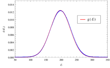
Figure 1: Continuous red curve represents the Gaussian distribution and blue dots represent the level density distribution of the spin chain (2.17) with $m_{1}=3$, $m_{2}=1$, $n_{1}=4$, $n_{2}=1$ and $N=20$.

Next, we shall study the distribution of spacing between consecutive energy levels for the spin chain (2.17). For the purpose of eliminating the effect of local level density variation in the distribution of spacing between energy levels, an unfolding mapping is usually employed to the ‘raw’ spectrum [65]. Since the level density of the spin chain (2.17) obeys Gaussian distribution for large number of lattice sites, one can express the corresponding cumulative level density $\eta(\mathcal{E})$ through the error function as

$$\eta(\mathcal{E})=\int_{-\infty}^{\mathcal{E}}G(x)dx=\frac{1}{2}\left[1+\rm{erf}\left(\frac{\mathcal{E}-\mu}{\surd{2}\sigma}\right)\right].$$ (7.8)

For the case of spin chain (2.17), this cumulative level density function is applied to map the energy levels $\mathcal{E}_{i},~{}~{}i=1,...,l$, into unfolded energy levels of the form $\eta_{i}\equiv\eta(\mathcal{E}_{i})$. The cumulative level spacing distribution for such unfolded energy levels is obtained through the relation

$$P(s)=\int_{0}^{s}p(x)dx\,,$$ (7.9)

where $p(s_{i})$ denotes the probability density of normalized spacing $s_{i}$ given by $s_{i}=(\eta_{i+1}-\eta_{i})/\Delta$ and $\Delta=(\eta_{l}-\eta_{1})/(͑l-1)$ is the mean spacing between unfolded energy levels. According to a well-known conjecture by Berry and Tabor, the density of normalized spacing for a ‘generic’ quantum integrable system should obey the Poisson’s law given by $p(s)=e^{-s}$ [66]. However, it has been observed earlier that $p(s)$ does not exhibit this Poissonian behaviour for a large class of quantum integrable spin chains with long-range interactions [12, 21, 22, 15, 61, 55].

To explain the above mentioned anomalous behaviour in the spectra of quantum integrable spin chains with long range interactions, it has been analytically shown in Ref. [22] that if the discrete spectrum of a quantum system satisfies the following four conditions:
i) the energy levels are equispaced, i.e., $\mathcal{E}_{i+1}-\mathcal{E}_{i}=\delta$, for $i=1,2,\ldots,l-1$,
ii) the level density is approximately Gaussian,
iii) $\mathcal{E}_{max}-\mu,~{}\mu-\mathcal{E}_{min}\gg\sigma$,
iv) $|\mathcal{E}_{max}+\mathcal{E}_{min}-2\mu|\ll\mathcal{E}_{max}-\mathcal{E}_{min}\,,$
then the corresponding cumulative level spacing distribution is approximately given by

$$\tilde{P}(s)\simeq 1-\frac{2}{\sqrt{\pi}s_{max}}\sqrt{\ln\left(\frac{s_{max}}{s}\right)}\,,$$ (7.10)

where

$$s_{max}=\frac{\mathcal{E}_{max}-\mathcal{E}_{min}}{\sqrt{2\pi}~{}\sigma}\,.$$ (7.11)

Since, the spectra of many quantum integrable spin chains with long-range interactions satisfy the above mentioned four conditions with reasonable accuracy, the cumulative level density of such spin chains obey the ‘square root of a logarithm’ law (7.10). In the case of presently considered spin chain (2.17), it has been already found that the conditions i) and ii) are satisfied. For the purpose of analyzing the remaining conditions, we use Eqs. (6.3), (6.4), (6.5) and (6.6) to obtain $\mathcal{E}_{min}=O(N)$ and $\mathcal{E}_{max}=N^{2}+O(N)$. Moreover, with the help of Eqs. (7.2) and (7.3), we find that

$$\mu=\frac{1}{2}\left(1-\frac{\tau_{3}}{\tau_{1}^{2}}\right)N^{2}+O(N),~{}~{}~{}~{}\sigma^{2}=\frac{1}{9}\left[1-\frac{\tau_{3}^{2}-32mn}{\tau_{1}^{4}}\right]N^{3}+O(N^{2}).$$

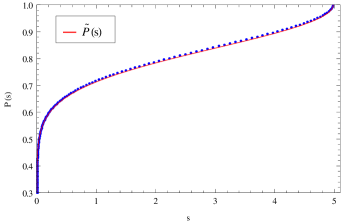
Figure 2: Blue dots represent cumulative level spacing distribution $P(s)$ for the spin chain with $m_{1}=3$, $m_{2}=1$, $n_{1}=4$, $n_{2}=1$ and $N=20$, while continuous red line is the corresponding analytic approximation $\tilde{P}(s)$.

Since $\tau_{1}=m+n$ and $\tau_{3}=m-n$, the leading order contributions to mean and variance in the above equation interestingly depend only on the values of $m$ and $n$. Using the leading order contributions to $\mathcal{E}_{min}$, $\mathcal{E}_{max}$, $\mu$ and $\sigma^{2}$, it is easy to check that the conditions iii) is also obeyed for the spectrum of the spin chain (2.17) with $N\gg 1$, whereas condition iv) holds only in the case when $m=n$. However, it can be shown that even if condition iv) is dropped, Eq. (7.10) is still obeyed within a slightly smaller range of $s$ [54]. Hence, it is expected that $P(s)$ in (7.9) would follow the analytical expression $\tilde{P}(s)$ in (7.10) for the case of spin chain (2.17). With the help of Mathematica, we compute $P(s)$ by taking different sets of positive integer values of $m_{1},~{}m_{2},~{}n_{1}$ and $n_{2}$ satisfying the conditions $|m_{1}-m_{2}|>1$ and $|n_{1}-n_{2}|>1$, and for moderately large values of $N$. It turns out that $P(s)$ obeys the analytical expression (7.10) with remarkable accuracy in all of these cases. As an example, in Fig. 2 we compare $P(s)$ with $\tilde{P}(s)$ for the particular case $m_{1}=3$, $m_{2}=1$, $n_{1}=4$, $n_{2}=1$ and $N=20$.

8 Conclusions

Here we construct SAPSRO which satisfy the $BC_{N}$ type of Weyl algebra and lead to a novel class of spin Calogero models as well as related PF chains with reflecting ends. We compute the exact spectra of these $BC_{N}$ type of spin Calogero models, by using the fact that their Hamiltonians can be represented in triangular forms while acting on some partially ordered sets of basis vectors of the corresponding Hilbert spaces. Since the strong coupling limit of these spin Calogero models yields $BC_{N}$ type of PF chains with SAPSRO, we apply the freezing trick to obtain the partition functions of this type of PF spin chains in a closed form. We also derive a formula (4.5) which expresses such a partition function in terms of known partition functions of several $A_{K}$ type of supersymmetric PF spin chains, where $K\leqslant N-1$. By using this formula, we analyze statistical properties like level density distribution and nearest neighbour spacings distribution in the spectra of spin chains with sufficiently large number of lattice sites. It turns out that, in analogy with the case of many other integrable systems with long-range interactions, the level density of PF spin chains with SAPSRO follows the Gaussian distribution and the cumulative nearest neighbour spacings distribution obeys the ‘square root of a logarithm’ law.

In this paper, we show that the partition functions of PF spin chains with SAPSRO obey an interesting type of duality relation. To this end, we consider a new quantum number which measures the parity of the spin states under the action of SAPSRO. It is found that the partition functions of these spin chains satisfy an ‘extended’ boson-fermion duality relation (5.13), which involves not only the exchange of bosonic and fermionic degrees of freedom, but also the exchange of positive and negative parity degrees of freedom associated with SAPSRO. As an application of this duality relation, we compute the highest energy levels of these spin chains from their ground state energies. Moreover, we find that partition functions of a large class of integrable and nonintegrable spin chains with Hamiltonians of the form (5.14) satisfy this type of duality relation.

We have mentioned earlier that, $BC_{N}$ type of PF spin chains with SAPSRO do not exhibit global su($m|n$) supersymmetry for arbitrary values of the related discrete parameters. However, for a particular choice of these discrete parameters, SAPSRO reduce to the trivial identity operator and lead to the su($m|n$) supersymmetric Hamiltonian $\mathcal{H}^{(m,0|n,0)}$ in (2.19). Curiously, we find that the partition function and spectrum of this $\mathcal{H}^{(m,0|n,0)}$ coincide with those of $A_{N-1}$ type of su($m|n$) supersymmetric PF chain with Hamiltonian $\widetilde{\mathcal{H}}_{\mathrm{PF}}^{(m|n)}$ in (4.7). Consequently, these two Hamiltonians are related through a unitary transformation of the form (4.9) and the spectrum of $\mathcal{H}^{(m,0|n,0)}$ can be expressed through Haldane’s motifs as given in (4.8). As a future study, it would be interesting to find out whether some modification of these motifs can be used to describe the spectra of $BC_{N}$ type of PF spin chains with SAPSRO for other possible choices of the related discrete parameters. It may also be noted that, $A_{N-1}$ type of PF chain with Hamiltonian $\widetilde{\mathcal{H}}_{\mathrm{PF}}^{(m|n)}$ in (4.7) exhibits the $Y(gl(m|n))$ super Yangian symmetry [9, 11]. Hence, due to the existence of unitary transformation (4.9), it is evident that the Hamiltonian $\mathcal{H}^{(m,0|n,0)}$ also exhibits the $Y(gl(m|n))$ super Yangian symmetry. However, finding out the explicit form for the conserved quantities of $\mathcal{H}^{(m,0|n,0)}$, which would satisfy the $Y(gl(m|n))$ algebra, remains an interesting problem on which work is currently in progress.

Acknowledgements

The authors thank Artemio González-López and Federico Finkel for fruitful discussions. One of the authors (B.B.M.) thanks the Abdus Salam International Centre for Theoretical Physics for a Senior Associateship, which partially supported this work.

References

• Haldane [1988] F. D. M. Haldane, Phys. Rev. Lett. 60 (1988) 635–638.
• Shastry [1988] B. S. Shastry, Phys. Rev. Lett. 60 (1988) 639–642.
• Haldane et al. [1992] F. D. M. Haldane, Z. N. C. Ha, J. C. Talstra, D. Bernard, V. Pasquier, Phys. Rev. Lett. 69 (1992) 2021–2025.
• Bernard et al. [1993] D. Bernard, M. Gaudin, F. D. M. Haldane, V. Pasquier, J. Phys. A: Math. Gen. 26 (1993) 5219–5236.
• Haldane [1994] F. D. M. Haldane, in: A. Okiji, N. Kawakami (Eds.), Correlation Effects in Low-dimensional Electron Systems, volume 118 of Springer Series in Solid-state Sciences, pp. 3–20.
• Polychronakos [1993] A. P. Polychronakos, Phys. Rev. Lett. 70 (1993) 2329–2331.
• Frahm [1993] H. Frahm, J. Phys. A: Math. Gen. 26 (1993) L473–L479.
• Polychronakos [1994] A. P. Polychronakos, Nucl. Phys. B 419 (1994) 553–566.
• Hikami [1995] K. Hikami, Nucl. Phys. B 441 (1995) 530–548.
• Basu-Mallick et al. [1999] B. Basu-Mallick, H. Ujino, M. Wadati, J. Phys. Soc. Jpn. 68 (1999) 3219–3226.
• Hikami and Basu-Mallick [2000] K. Hikami, B. Basu-Mallick, Nucl. Phys. B 566 (2000) 511–528.
• Finkel and González-López [2005] F. Finkel, A. González-López, Phys. Rev. B 72 (2005) 174411(6).
• Basu-Mallick and Bondyopadhaya [2006] B. Basu-Mallick, N. Bondyopadhaya, Nucl. Phys. B 757 (2006) 280–302.
• Basu-Mallick et al. [2008] B. Basu-Mallick, N. Bondyopadhaya, D. Sen, Nucl. Phys. B 795 (2008) 596–622.
• Barba et al. [2008] J. C. Barba, F. Finkel, A. González-López, M. A. Rodríguez, Europhys. Lett. 83 (2008) 27005(6).
• Enciso et al. [2010] A. Enciso, F. Finkel, A. González-López, Phys. Rev. E 82 (2010) 051117.
• Basu-Mallick et al. [2010] B. Basu-Mallick, N. Bondyopadhaya, K. Hikami, SIGMA 6 (2010) 091–13.
• Simons and Altshuler [1994] B. D. Simons, B. L. Altshuler, Phys. Rev. B 50 (1994) 1102–1105.
• Bernard et al. [1995] D. Bernard, V. Pasquier, D. Serban, Europhys. Lett. 30 (1995) 301–306.
• Yamamoto and Tsuchiya [1996] T. Yamamoto, O. Tsuchiya, J. Phys. A: Math. Gen. 29 (1996) 3977–3984.
• Enciso et al. [2005] A. Enciso, F. Finkel, A. González-López, M. A. Rodríguez, Nucl. Phys. B 707 (2005) 553–576.
• Barba et al. [2008] J. C. Barba, F. Finkel, A. González-López, M. A. Rodríguez, Phys. Rev. B 77 (2008) 214422(10).
• Ha [1996] Z. N. C. Ha, Quantum Many-body Systems in one Dimension, volume 12 of Advances in Statistical Mechanics, World Scientific, Singapore, 1996.
• Kuramoto and Kato [2009] Y. Kuramoto, Y. Kato, Dynamics of one-dimensional quantum systems: inverse-square interaction models, Cambridge Studies in Advanced Mathematics 29, Cambridge University Press, New York, 2009.
• Polychronakos [2006] A. P. Polychronakos, J. Phys. A: Math. Gen. 39 (2006) 12793–12845.
• Azuma and Iso [1994] H. Azuma, S. Iso, Phys. Lett. B 331 (1994) 107–113.
• Beenakker and Rajaei [1994] C. W. J. Beenakker, B. Rajaei, Phys. Rev. B 49 (1994) 7499–7510.
• Caselle [1995] M. Caselle, Phys. Rev. Lett. 74 (1995) 2776–2779.
• Beisert et al. [2003] N. Beisert, C. Kristjansen, M. Staudacher, Nucl. Phys. B 664 (2003) 131–184.
• Beisert [2004] N. Beisert, Nucl. Phys. B 682 (2004) 487–520.
• Bargheer et al. [2009] T. Bargheer, N. Beisert, F. Loebbert, J. Phys. A: Math. Theor. 42 (2009) 285205(58).
• Dunkl [1998] C. F. Dunkl, Commun. Math. Phys. 197 (1998) 451–487.
• Finkel et al. [2001] F. Finkel, D. Gómez-Ullate, A. González-López, M. A. Rodríguez, R. Zhdanov, Commun. Math. Phys. 221 (2001) 477–497.
• Taniguchi et al. [1995] N. Taniguchi, B. S. Shastry, B. L. Altshuler, Phys. Rev. Lett. 75 (1995) 3724–3727.
• Basu-Mallick [1999] B. Basu-Mallick, Nucl. Phys. B 540 (1999) 679–704.
• Basu-Mallick et al. [2007] B. Basu-Mallick, N. Bondyopadhaya, K. Hikami, D. Sen, Nucl. Phys. B 782 (2007) 276–295.
• Beisert and Erkal [2008] N. Beisert, D. Erkal, J. Stat. Mech. 0803 (2008) P03001.
• Cirac and Sierra [2010] J. I. Cirac, G. Sierra, Phys. Rev. B 81 (2010) 104431(4).
• Nielsen et al. [2011] A. Nielsen, J. I. Cirac, G. Sierra, J. Stat. Mech. (2011) P11014.
• Tu et al. [2014] H.-H. Tu, A. E. B. Nielsen, G. Sierra, Nucl. Phys. B 886 (2014) 328–363.
• Bondesan and Quella [2014] R. Bondesan, T. Quella, Nucl. Phys. B 886 (2014) 483–523.
• Gutzwiller [1963] M. C. Gutzwiller, Phys. Rev. Lett. 10 (1963) 159–162.
• Gebhard and Vollhardt [1987] F. Gebhard, D. Vollhardt, Phys. Rev. Lett. 59 (1987) 1472–1475.
• Gros et al. [1987] C. Gros, R. Joynt, T. M. Rice, Phys. Rev. B 36 (1987) 381–393.
• Sutherland and Shastry [1993] B. Sutherland, B. S. Shastry, Phys. Rev. Lett. 71 (1993) 5–8.
• Schlottmann [1997] P. Schlottmann, Int. Jour. Mod. Phys. B 11 (1997) 355.
• Saleur [2000] H. Saleur, Nucl. Phys. B 578 (2000) 552–576.
• Essler et al. [2005] F. Essler, H. Frahm, H. Saleur, Nucl. Phys. B 712 (2005) 513–572.
• Arikawa et al. [2001] M. Arikawa, Y. Saiga, Y. Kuramoto, Phys. Rev. Lett. 86 (2001) 3096–3099.
• Thomale et al. [2007] R. Thomale, D. Schuricht, M. Greiter, Phys. Rev. B 75 (2007) 024405.
• Basu-Mallick et al. [2009] B. Basu-Mallick, F. Finkel, A. González-López, Nucl. Phys. B 812 (2009) 402–423.
• Basu-Mallick et al. [2011] B. Basu-Mallick, F. Finkel, A. González-López, Nucl. Phys. B 843 (2011) 505–553.
• Basu-Mallick et al. [2013] B. Basu-Mallick, F. Finkel, A. González-López, Nucl. Phys. B 866 (2013) 391–413.
• Barba et al. [2009] J. C. Barba, F. Finkel, A. González-López, M. A. Rodríguez, Nucl. Phys. B 806 (2009) 684–714.
• Basu-Mallick et al. [2014] B. Basu-Mallick, N. Bondyopadhaya, P. Banerjee, Nucl. Phys. B 883 (2014) 501–528.
• Corrigan and Sasaki [2002] E. Corrigan, R. Sasaki, J. Phys. A: Math. Gen. 35 (2002) 7017–7061.
• Humphreys [1990] J. E. Humphreys, Reflection Groups and Coxeter Groups, Cambridge Studies in Advanced Mathematics 29, Cambridge University Press, Cambridge, 1990.
• Finkel et al. [2003] F. Finkel, D. Gómez-Ullate, A. González-López, M. A. Rodríguez, R. Zhdanov, Commun. Math. Phys. 233 (2003) 191–209.
• Caudrelier and Crampé [2004] V. Caudrelier, N. Crampé, J. Phys. A: Math. Gen. 37 (2004) 6285–6298.
• Cigler [1979] J. Cigler, Monatsh. Math. 88 (1979) 87–105.
• Basu-Mallick and Bondyopadhaya [2009] B. Basu-Mallick, N. Bondyopadhaya, Phys. Lett. A 373 (2009) 2831–2836.
• Banerjee and Basu-Mallick [2012] P. Banerjee, B. Basu-Mallick, J. Math. Phys. 53 (2012) 083301.
• Ahmed [1978] S. Ahmed, Lett. Nuovo Cimento 22 (1978) 371–375.
• Ahmed and Muldoon [1983] S. Ahmed, M. E. Muldoon, SIAM J. Math. Anal. 14 (1983) 372–382.
• Haake [2001] F. Haake, Quantum Signatures of Chaos, Springer-Verlag, Berlin, second edition, 2001.
• Berry and Tabor [1977] M. V. Berry, M. Tabor, Proc. R. Soc. London Ser. A 356 (1977) 375–394.