Quantum Teichmüller spaces and quantum trace map

Abstract.

We show how the quantum trace map of Bonahon and Wong can be constructed in a natural way using the skein algebra of Muller, which is an extension of the Kauffman bracket skein algebra of surfaces. We also show that the quantum Teichmüller space of a marked surface, defined by Chekhov-Fock (and Kashaev) in an abstract way, can be realized as a concrete subalgebra of the skew field of the skein algebra.

1. Introduction

1.1. Quantum trace map for triangulated marked surfaces

Suppose $(\Sigma,\mathcal{P})$ is marked surface, i.e. $\Sigma$ is an oriented connected compact surface with boundary $\partial\Sigma$ and $\mathcal{P}\subset\partial\Sigma$ is finite set of marked points. F. Bonahon and H. Wong [BW1] constructed a remarkable injective algebra homomorphism, called the quantum trace map

(1) $$\operatorname{\mathrm{t}r}_{q}^{\Delta}:\mathring{\mathscr{S}}\to\mathcal{Y}^{\mathrm{bl}}(\Delta),$$

where $\mathring{\mathscr{S}}$ is the Kauffman bracket skein algebra of $\Sigma$ and $\mathcal{Y}^{\mathrm{bl}}(\Delta)$ is the square root version of the Chekhov-Fock algebra of $(\Sigma,\mathcal{P})$. We recall the definitions of $\mathring{\mathscr{S}}$ and $\mathcal{Y}^{\mathrm{bl}}(\Delta)$ in Section 5. While the skein algebra $\mathring{\mathscr{S}}$ does not depend on $\mathcal{P}$ nor any triangulation, the square root Chekhov-Fock algebra $\mathcal{Y}^{\mathrm{bl}}(\Delta)$ depends on a $\mathcal{P}$-triangulation $\Delta$ of $\Sigma$, i.e. a triangulation whose set of vertices is $\mathcal{P}$.

The skein algebra $\mathring{\mathscr{S}}$ was introduced by J. Przytycki [Pr] and V. Turaev [Tu] based on the Kauffman bracket [Kau], and is a quantization of the $SL_{2}$-character variety of $\Sigma$ along the Goldman-Weil-Petersson Poisson form, see [BFK, Bu2, PS, Tu]. The Chekhov Fock algebra in our paper is the multiplicative version of the one originally defined by Chekhov and Fock [CF1]. The theory of this multiplicative version and its square root version was developed by Bonahon, Liu, and Hiatt [BL, Liu, Hi]. The Chekhov-Fock algebra is a quantization of the enhanced Teichmüller space using Thurston’s shear coordinates, also along the Goldman-Weil-Petersson Poisson form. A slightly different form of a quantization of the enhanced Teichmüller space using shear coordinates is also introduced by Kashaev [Kas].

Based on the close relation between the $SL_{2}$-character variety and the Teichmm̈uller space, V. Fock [Fo] and Chekhov and Fock [CF2] made a conjecture that a quantum trace map as in Equation (1) exists. The conjecture was proved in special cases in [CP, Hi] and in full generality by Bonahon and Wong [BW1]. When the quantum parameter $q$ is set to 1, the quantum trace map expresses the $SL_{2}$-trace of a loop in terms of the shear coordinates.

Skein algebras of surfaces, or more generally skein modules of 3-manifolds, are objects which can be defined using simple geometric notions but are hard to deal with since their algebra is difficult to handle. Their geometric definition helps to relate skein algebras/modules to topological objects like the fundamental groups, the Jones polynomial, etc. For example, understanding the skein modules of knot complements can help to prove the AJ conjecture, which relates the Jones polynomial and the fundamental group of a knot [Le1, LT, LZ], and the skein modules are used in the construction of topological quantum field theories [BHMV]. The introduction of the quantum trace map is a breakthrough in the study of skein algebras; it embeds the skein algebra $\mathring{\mathscr{S}}$ into quantum tori which have simple algebraic structure. For example, representations of $\mathring{\mathscr{S}}$ are studied via the quantum trace map in [BW2]. We will use quantum trace maps to the study of skein modules of knot complements in future work.

1.2. Quantum trace map through the Muller algebra in skein theory

The original construction of the quantum trace map in [BW1] involves difficult calculations, with miraculous identities. One of the goals of this paper is to offer another approach to the quantum trace map of Bonahon and Wong using Muller’s extension of skein algebras. By extending the definition of skein algebras to the class of marked surfaces [Mu], we have a natural embedding of the skein algebra $\mathring{\mathscr{S}}$ of $\Sigma$ into the skein algebra $\mathscr{S}$ of the marked surface $(\Sigma,\mathcal{P})$. The latter, in the presence of a $\mathcal{P}$-triangulation $\Delta$, naturally contains the positive part $\mathfrak{X}_{++}(\Delta)$ of a nice algebra $\mathfrak{X}(\Delta)$, called the Muller algebra, which is a quantum torus (see Section 5 for details). Muller showed that the inclusion $\mathfrak{X}_{++}(\Delta)\subset\mathscr{S}$ leads to a natural embedding $\varphi_{\Delta}:\mathring{\mathscr{S}}\hookrightarrow\mathfrak{X}(\Delta)$. And we want to argue that $\varphi_{\Delta}:\mathring{\mathscr{S}}\hookrightarrow\mathfrak{X}(\Delta)$ is the same as the quantum trace map of Bonahon and Wong, via the quantum shear-to-skein map as follows.

The Muller algebra $\mathfrak{X}(\Delta)$ is a quantum torus, constructed based on the vertex matrix of $(\Sigma,\mathcal{P})$ (see Sections 2 and 5). The algebra $\mathcal{Y}^{\mathrm{bl}}(\Delta)$ is a subalgebra of another quantum torus based on the face matrix of $(\Sigma,\mathcal{P})$. Using a duality between the vertex matrix and the face matrix, we construct an embedding $\psi:\mathcal{Y}^{\mathrm{bl}}(\Delta)\hookrightarrow\mathfrak{X}(\Delta)$. Now we have two embeddings into $\mathfrak{X}(\Delta)$:

(2) $$\mathring{\mathscr{S}}\overset{\varphi_{\Delta}}{\lhook\joinrel\relbar\joinrel\rightarrow}\mathfrak{X}(\Delta)\overset{\psi}{\leftarrow\joinrel\relbar\joinrel\rhook}\mathcal{Y}^{\mathrm{bl}}(\Delta).$$

Theorem 1.

In Diagram (2), the image of $\psi$ contains the image of $\varphi_{\Delta}$. The injective algebra homomorphism $\varkappa_{\Delta}:\mathring{\mathscr{S}}\to\mathcal{Y}^{\mathrm{bl}}(\Delta)$ defined by $\varkappa_{\Delta}:=\psi^{-1}\circ\varphi_{\Delta}$ is equal to the quantum trace map of Bonahon and Wong.

The map $\psi$ could be considered as a kind of Fourier transform, as it relates two types of coordinates based to matrices which are almost dual to each other. When the quantum parameter is set to 1, $\psi$ becomes the map expressing the shear coordinates in terms of Penner coordinates in the decorated Teichmüller space [Pe]. One can show that the Muller algebra is the exponential version of the Moyal quantization of the decorated Teichmüller space of the marked surface with respect to a natural linear Poisson structure. Theorem 1 is proved in Section 6.

1.3. The quantum Teichmüller space

To each triangulation $\Delta$ of a marked surface $(\Sigma,\mathcal{P})$, Chekhov and Fock defined an algebra, denoted by $\mathcal{Y}^{(2)}(\Delta)$ in this paper, which is a subalgebra of the square root version $\mathcal{Y}^{\mathrm{bl}}(\Delta)$ (see Section 6). To define an object not depending on triangulations, Chekhov and Fock suggested the following approach.

Being a quantum torus, $\mathcal{Y}^{(2)}(\Delta)$ is a two-sided Ore domain and hence has a skew field $\tilde{\mathcal{Y}}^{(2)}(\Delta)$ (see Section 2). It was proved [CF1, Liu] that for any two triangulations $\Delta,\Delta^{\prime}$ there is a natural change of coordinate isomorphism $\Theta_{\Delta\Delta^{\prime}}:\tilde{\mathcal{Y}}^{(2)}(\Delta^{\prime})\to\tilde{\mathcal{Y}}^{(2)}(\Delta)$. Naturality means $\Theta_{\Delta\Delta}={\mathrm{id}}$ and $\Theta_{\Delta\Delta^{\prime\prime}}=\Theta_{\Delta\Delta^{\prime}}\circ\Theta_{\Delta^{\prime}\Delta^{\prime\prime}}$ for any 3 triangulations $\Delta,\Delta^{\prime},\Delta^{\prime\prime}$. Then one defines $\mathcal{T}=\sqcup_{\Delta}\tilde{\mathcal{Y}}^{(2)}(\Delta)/\sim$, where $\sim$ is the equivalence relation defined by $a\sim b$, where $a\in\tilde{\mathcal{Y}}^{(2)}(\Delta)$ and $b\in\tilde{\mathcal{Y}}^{(2)}(\Delta^{\prime})$, if $a=\Theta_{\Delta\Delta^{\prime}}(b)$. The algebra $\mathcal{T}$ is called the quantum Teichmüller space of $(\Sigma,\mathcal{P})$. This approach defines $\mathcal{T}$ in an abstract way.

Using the skein algebra $\mathscr{S}$ of $(\Sigma,\mathcal{P})$, we are able to realize $\mathcal{T}$ as a concrete subspace of the skew field $\tilde{\mathscr{S}}$ of $\mathscr{S}$. First, Muller [Mu] shows that the embedding $\varphi_{\Delta}:\mathscr{S}\hookrightarrow\mathfrak{X}(\Delta)$ extends to an isomorphism of skew fields $\tilde{\varphi}_{\Delta}:\tilde{\mathscr{S}}\overset{\cong}{\longrightarrow}\tilde{\mathfrak{X}}(\Delta)$. Besides, the embedding $\psi:\mathcal{Y}^{(2)}(\Delta)\hookrightarrow\mathfrak{X}(\Delta)$ extends to $\tilde{\psi}:\tilde{\mathcal{Y}}^{(2)}(\Delta)\hookrightarrow\tilde{\mathfrak{X}}(\Delta)$. This leads to an embedding

$$\tilde{\psi}_{\Delta}:=(\tilde{\varphi}_{\Delta})^{-1}\circ\tilde{\psi}:\tilde{\mathcal{Y}}^{(2)}(\Delta)\hookrightarrow\tilde{\mathscr{S}}.$$

Theorem 2.

The image $\tilde{\mathscr{S}}^{(2)}:=\tilde{\psi}_{\Delta}(\tilde{\mathcal{Y}}^{(2)}(\Delta))$ in $\tilde{\mathscr{S}}$ does not depend on the triangulation $\Delta$, and the coordinate change map $\Theta_{\Delta\Delta^{\prime}}$ is equal to $(\tilde{\psi}_{\Delta})^{-1}\circ\tilde{\psi}_{\Delta^{\prime}}$. Here $(\tilde{\psi}_{\Delta})^{-1}$ is defined on $\tilde{\mathscr{S}}^{(2)}$.

Thus, $\tilde{\mathscr{S}}^{(2)}$ is a concrete realization of the quantum Teichmüller space $\mathcal{T}$, not depending on any triangulation. We also give an intrinsic characterization of $\tilde{\mathscr{S}}^{(2)}$ using $\mathcal{P}$-quadrilaterals, see Section 6. From this point of view, the construction of the coordinate change isomorphism is natural. Theorem 2 is part of Theorem 6.6, which contains also similar statements for the square root version $\mathcal{Y}^{\mathrm{bl}}(\Delta)$.

1.4. Punctured surfaces and more general surfaces

Suppose ${\mathfrak{S}}$ is a punctured surface which is obtained from a closed oriented connected surface $\bar{{\mathfrak{S}}}$ by removing a finite set $\mathcal{P}$. The skein algebra $\mathring{\mathscr{S}}$ of ${\mathfrak{S}}$ and the square root Chekhov-Fock algebra $\mathcal{Y}^{\mathrm{bl}}({\Lambda})$ (depending on an ideal triangulation ${\Lambda}$ of ${\mathfrak{S}}$) are defined as usual. Bonahon and Wong also showed that the quantum trace map (an injective algebra homomorphism)

$$\operatorname{\mathrm{t}r}_{q}^{\Lambda}:\mathring{\mathscr{S}}\to\mathcal{Y}^{\mathrm{bl}}({\Lambda}),$$

exists in this case. However, since ${\mathfrak{S}}$ is not a marked surface in the sense of [Mu], the Muller algebra cannot be defined in this case.

To remedy this, we introduce a marked surface $(\Sigma,\mathcal{P})$ associated to ${\mathfrak{S}}$ as follows. For each $p\in\mathcal{P}$ let $D_{p}\subset\bar{{\mathfrak{S}}}$ be a small disk such that $p\in\partial D_{p}$. Removing the interior of each disk $D_{p}$ from $\bar{{\mathfrak{S}}}$ we get $\Sigma$, which together with $\mathcal{P}$ forms a marked surface $(\Sigma,\mathcal{P})$. The skein algebra of $\Sigma$ and that of ${\mathfrak{S}}$ are naturally identified and denoted by $\mathring{\mathscr{S}}$. Every $\mathcal{P}$-triangulation ${\Lambda}$ of $\bar{{\mathfrak{S}}}$ can be extended to a $\mathcal{P}$-triangulation $\Delta$ of $\Sigma$. The Muller algebra $\mathfrak{X}(\Delta)$ of $(\Sigma,\mathcal{P})$ contains a subalgebra $\bar{\mathfrak{X}}(\Delta)$ which is built by the standard generators of $\mathfrak{X}(\Delta)$ excluding the boundary elements. There is a natural projection $\pi:\mathfrak{X}(\Delta)\to\bar{\mathfrak{X}}(\Delta)$, see Section 8. Define ${\bar{\varphi}_{\Delta}}=\pi\circ\varphi_{\Delta}:\mathring{\mathscr{S}}\to\bar{\mathfrak{X}}(\Delta)$. The shear-to-skein map $\bar{\psi}:\mathcal{Y}^{\mathrm{bl}}({\Lambda})\hookrightarrow\bar{\mathfrak{X}}(\Delta)$ can be defined using the map $\psi:\mathcal{Y}^{\mathrm{bl}}(\Delta)\hookrightarrow\mathfrak{X}(\Delta)$. We will show that the quantum trace map of Bonahon and Wong is equal to ${\bar{\varphi}_{\Delta}}:\mathring{\mathscr{S}}\to\bar{\mathfrak{X}}(\Delta)$, via the shear-to-skein map $\bar{\psi}$.

Theorem 3.

In the diagram

$$\mathring{\mathscr{S}}\overset{{\bar{\varphi}_{\Delta}}}{\longrightarrow}\bar{\mathfrak{X}}(\Delta)\overset{\bar{\psi}}{\leftarrow\joinrel\relbar\joinrel\rhook}\mathcal{Y}^{\mathrm{bl}}({\Lambda})$$

the image of $\bar{\psi}$ contains the image of ${\bar{\varphi}_{\Delta}}$. The algebra homomorphism $\bar{\varkappa}_{\Lambda}:\mathring{\mathscr{S}}\to\mathcal{Y}^{\mathrm{bl}}(\Delta)$ defined by $\bar{\varkappa}_{\Lambda}:=\bar{\psi}^{-1}\circ{\bar{\varphi}_{\Delta}}$ is equal to the quantum trace map of Bonahon and Wong.

Theorem 3 is a special case of Theorem 8.8, which treats more general type of punctured surfaces.

1.5. Organization of the paper

Section 2 presents the basics of quantum tori, including multiplicative homomorphisms which help to define the shear-to-skein maps later. In Section 3 we introduce the notion of skein modules of a marked 3-manifolds. Section 4 discusses the basics of marked surfaces, including the duality between the face and the vertex matrix. In Section 5 we calculate the image of simple knot under $\varphi_{\Delta}$, a crucial technical step. In Sections 6 and 8 we prove the main results, while in Section 7 the quantum trace of a class of simple knots is calculated. In the Appendix we prove Theorem 6.6.

1.6. Acknowledgements

The author would like to thank F. Bonahon, C. Frohman, A. Kricker, G. Masbaum, G. Muller, J. Paprocki, A. Sikora, and D. Thurston for helpful discussions. The author would also like to thank Centre for Quantum Geometry of Moduli Spaces (Arhus) and University of Zurich, where part of this work was done, for their support and hospitality.

2. Quantum torus

In this paper $\mathbb{N},\mathbb{Z},\mathbb{Q}$ are respectively the set of non-negative integers, the set of integers, and the set of rational numbers. Besides, $q^{1/8}$ is a formal parameter and ${\mathcal{R}}=\mathbb{Z}[q^{\pm 1/8}]$.

2.1. Non-commutative product and Weyl normalization

Suppose ${\mathcal{A}}$ is an ${\mathcal{R}}$-algebra, not necessarily commutative. Two element $x,y\in{\mathcal{A}}$ are said to be $q$-commuting if there is $\mathcal{C}(x,y)\in\mathbb{Q}$ such that $xy=q^{\mathcal{C}(x,y)}yx$. Suppose $x_{1},x_{2},\dots,x_{n}\in{\mathcal{A}}$ are pairwise $q$-commuting with $\mathcal{C}(x_{i},x_{j})\in\frac{1}{4}\mathbb{Z}$, the Weyl normalization of $\prod_{i}x_{i}$ is defined by

$$\left[x_{1}x_{2}\dots x_{n}\right]:=q^{-\frac{1}{2}\sum_{i<j}\mathcal{C}(x_{i},x_{j})}x_{1}x_{2}\dots x_{n}.$$

It is known that the normalized product does not depend on the order, i.e. if $(y_{1},y_{2},\dots,y_{n})$ is a permutation of $(x_{1},x_{2},\dots,x_{n})$, then $[y_{1}y_{2}\dots y_{n}]=[x_{1}x_{2}\dots x_{n}]$.

2.2. Quantum torus

Let $I,J$ be finite sets. Denote by $\mathrm{Mat}(I\times J,\mathbb{Z})$ the set of all $I\times J$ matrices with entries in $\mathbb{Z}$, i.e. $A\in\mathrm{Mat}(I\times J,\mathbb{Z})$ is a function $A:I\times J\to\mathbb{Z}$. We write $A_{ij}$ for $A(i,j)$.

We say $A\in\mathrm{Mat}(I\times I,\mathbb{Z})$ is antisymmetric if $A_{ij}=-A_{ji}$. Assume $A\in\mathrm{Mat}(I\times I,\mathbb{Z})$ is antisymmetric and $u=q^{m/4}$ for some $m\in\mathbb{Z}$. Let $u^{1/2}=q^{m/8}$. Define the quantum torus over ${\mathcal{R}}$ associated to $(A,u)$ by

$$\mathbb{T}(A,u,x):=R\langle x_{i}^{\pm 1},i\in I\rangle/(x_{i}x_{j}=u^{A_{ij}}x_{j}x_{i}).$$

We call $x_{i},i\in I$ the basis variables of the quantum torus $\mathbb{T}(A,u,x)$. Letter $x$ indicates that the basis variables are $x_{i},i\in I$. We often write $\mathbb{T}(A,u)=\mathbb{T}(A,u,x)$ when the basis variables are fixed.

It is known that $\mathbb{T}(A,u)$ is a two-sided Noetherian domain, and hence a two-sided Ore domain, see e.g. [GW]. Denote by $\tilde{\mathbb{T}}(A,u)$ the skew field (or division algebra) of $\mathbb{T}(A,u)$.

Let $\mathbb{Z}^{I}$ be the set of all maps $\mathbf{k}:I\to\mathbb{Z}$. For $\mathbf{k}\in\mathbb{Z}^{I}$ define the normalized monomial $x^{\mathbf{k}}$ by

$$x^{\mathbf{k}}=\left[\prod_{i\in I}x_{i}^{\mathbf{k}(i)}\right].$$

The set $\{x^{\mathbf{k}}\mid\mathbf{k}\in\mathbb{Z}^{I}\}$ is an ${\mathcal{R}}$-basis of $\mathbb{T}(A,u,x)$.

We will consider $\mathbf{k}\in\mathbb{Z}^{I}$ as a row vector, i.e. a matrix of size $1\times I$. Let $\mathbf{k}^{\dagger}$ be the transpose of $\mathbf{k}$. Define an anti-symmetric $\mathbb{Z}$-bilinear form on $\mathbb{Z}^{I}$ by

$$\langle\mathbf{k},\mathbf{n}\rangle_{A}:=\sum A_{ij}\mathbf{k}(i)\mathbf{n}(j)=\mathbf{k}A\mathbf{n}^{\dagger}.$$

The following well-known fact follows easily from the definition.

Proposition 2.1.

For $\mathbf{k},\mathbf{n},\mathbf{k}_{1},\dots,\mathbf{k}_{m}\in\mathbb{Z}^{I}$, one has

(3) $$x^{\mathbf{k}}x^{\mathbf{n}} =u^{\langle\mathbf{k},\mathbf{n}\rangle_{A}}\,x^{\mathbf{n}}x^{\mathbf{k}}$$

(4) $$x^{\mathbf{k}_{1}}x^{\mathbf{k}_{2}}\dots x^{\mathbf{k}_{m}} =u^{\frac{1}{2}\sum_{j<l}\langle\mathbf{k}_{j},\mathbf{k}_{l}\rangle_{A}}\,x^{\sum_{j}\mathbf{k}_{j}}.$$

In particular, for $n\in\mathbb{Z}$ and $\mathbf{k}\in\mathbb{Z}^{I}$, one has $(x^{\mathbf{k}})^{n}=x^{n\mathbf{k}}$.

Remark 2.2.

The quantum torus $\mathbb{T}(A,u,x)$ can be defined as the free ${\mathcal{R}}$-module with basis $\{x^{\mathbf{k}}\mid\mathbf{k}\in\mathbb{Z}^{I}\}$ subject to the relation (3).

2.3. Reflection symmetry

There is a unique $\mathbb{Z}$-algebra anti-homomorphism

$$\chi:\mathbb{T}(A,u,x)\to\mathbb{T}(A,u,x)$$

satisfying

$$\chi(q^{1/8})=q^{-1/8},\quad\chi(x_{i})=x_{i}\ \forall i\in I.$$

Here $\chi$ is an algebra anti-homomorphism means $\chi(xy)=\chi(y)\chi(x)$ for all $x,y\in\mathbb{T}(A,u)$. Note that $\chi$ is an anti-involution of $\mathbb{T}(A,u)$ since $\chi^{2}={\mathrm{id}}$. We call $\chi$ the reflection symmetry. It is clear that $\chi$ extends to an anti-involution of $\tilde{\mathbb{T}}(A,u)$.

An element $z\in\mathbb{T}(A,u)$ is called reflection invariant if $\chi(z)=z$. Similarly, if $A\in\mathrm{Mat}(I\times I,\mathbb{Z})$ and $B\in\mathrm{Mat}(J\times J,\mathbb{Z})$ are antisymmetric matrices, an ${\mathcal{R}}$-algebra homomorphism $f:\mathbb{T}(A,u)\to\mathbb{T}(B,v)$ is said to be reflection invariant if $f\chi=\chi f$.

From the definition, one sees that each normalized monomial $x^{\mathbf{k}}$ is reflection invariant. The following simple fact will be helpful and used many times.

Lemma 2.3.

Suppose in $z\in\mathbb{T}(A,u)$ is reflection invariant and

(5) $$z=\sum_{j=1}^{m}q^{r_{j}}x^{\mathbf{k}_{j}},$$

where $r_{j}\in\mathbb{Q}$, and $\mathbf{k}_{j}$ are pairwise distinct. Then all $r_{j}=0$, i.e. $z=\sum_{j=1}^{m}x^{\mathbf{k}_{j}}.$

Proof.

Applying $\chi$ to (5), we have $z=\sum_{j=1}^{m}q^{-r_{j}}x^{\mathbf{k}_{j}}.$ Since $k_{j}$ are pairwise distinct, the presentation of $z$ as a linear combination of $x^{\mathbf{k}_{j}}$ is unique. Hence we must have $q^{r_{j}}=q^{-r_{j}}$, or $r_{j}=0$. ∎

Remark 2.4.

Lemma 2.3 is one reason why we use $q$ as an indeterminate, not a complex number.

2.4. Based modules

A based ${\mathcal{R}}$-module $(V,\mathcal{B})$ consists of a free ${\mathcal{R}}$-module $V$ and a preferred base $\mathcal{B}$. Another based module $(V^{\prime},\mathcal{B}^{\prime})$ is a based submodule of $(V,\mathcal{B})$ if $V^{\prime}\subset V$ and $\mathcal{B}^{\prime}\subset\mathcal{B}$. In that case, the canonical projection $\pi:V\to V^{\prime}$ is the ${\mathcal{R}}$-linear map given by $\pi(v)=v$ if $v\in\mathcal{B}^{\prime}$ and $\pi(v)=0$ if $v\in\mathcal{B}\setminus\mathcal{B}^{\prime}$. The following is obvious and will be useful.

Lemma 2.5.

Let $(V^{\prime},\mathcal{B}^{\prime})$ be a based submodule of $(V,\mathcal{B})$. Suppose $a\in V^{\prime}$ and $a=\sum_{j=1}^{m}q^{r_{j}}b_{j},$ where each $b_{j}\in\mathcal{B}$ and $r_{j}\in\mathbb{Q}$. Then $b_{j}\in\mathcal{B}^{\prime}\subset V^{\prime}$ for every $j=1,\dots,m$.

For an anti-symmetric matrix $A\in\mathrm{Mat}(I\times I,\mathbb{Z})$, we will consider the quantum torus $\mathbb{T}(A,u,x)$ as a based module with the preferred base $\{x^{\mathbf{k}}\mid\mathbf{k}\in\mathbb{Z}^{I}\}$. Suppose $I^{\prime}\subset I$ and $A^{\prime}$ is the $I^{\prime}\times I^{\prime}$ submatrix of $A$. Then $\mathbb{T}(A^{\prime},u)$ is a based submodule of $\mathbb{T}(A,u)$. The canonical projection is not an algebra homomorphism unless $A^{\prime}=A$. However, if $V$ is the ${\mathcal{R}}$-submodule of $\mathbb{T}(A,u)$ spanned by $x^{\mathbf{k}}$ such that $\mathbf{k}(i)\geq 0\ \forall i\in I\setminus I^{\prime}$, then the restriction of $\pi$ onto $V$ is an algebra homomorphism.

2.5. Multiplicatively linear homomorphism

Suppose $A\in\mathrm{Mat}(I\times I,\mathbb{Z})$ and $B\in\mathrm{Mat}(J\times J,\mathbb{Z})$ are antisymmetric matrices, and both $u,u^{r}$ are integral powers of $q^{1/4}$, for some rational number $r$. Consider the quantum tori $\mathbb{T}(A,u^{r},x)$ and $\mathbb{T}(B,u,y)$.

For a matrix $H\in\mathrm{Mat}(I\times J,\mathbb{Z})$, define an ${\mathcal{R}}$-linear map

$$\psi=\psi_{H}:\mathbb{T}(A,u^{r},x)\to\mathbb{T}(B,u,y),\quad\text{by }\ \psi(x^{\mathbf{k}}):=y^{\mathbf{k}H}.$$

Denote by $H^{\dagger}$ the transpose of $H$.

Proposition 2.6.

(a) The above defined $\psi$ is a ${\mathcal{R}}$-algebra homomorphism if and only if

(6) $$HBH^{\dagger}=rA.$$

(b) The map $\psi$ is reflection invariant.

(c) Suppose $\mathrm{rk}(H)=|I|$. Then $\psi$ is injective.

Proof.

(a) follows right away from (3). See Remark 2.2.

(b) Since $x^{\mathbf{k}}$ and $y^{\mathbf{k}H}$ are reflection invariant, $\psi$ is reflection invariant.

(c) Since $\mathrm{rk}(H)=|I|$, $\psi$ maps injectively the preferred base of $\mathbb{T}(A,u^{r})$ into the preferred base of $\mathbb{T}(B,u)$. Hence, $\psi$ is injective. ∎

In case $\mathrm{rk}(H)=|I|$, a left inverse of $\psi$ can be given by a multiplicative linear homomorphism.

3. Skein modules of 3-manifolds

3.1. Marked 3-manifold

A marked 3-manifold $(M,\mathcal{N})$ consists of an oriented connected 3-manifold $M$ with (possibly empty) boundary $\partial M$ and a 1-dimensional oriented submanifold $\mathcal{N}\subset\partial M$ such that $\mathcal{N}$ is the disjoint union of several open intervals. Here an open interval in $\partial M$ is an oriented 1-dimensional submanifold of $\partial M$ diffeomorphic to the interval $(0,1)$.

An $\mathcal{N}$-link $L$ (in $M$) is a compact 1-dimensional non-oriented smooth submanifold of $M$ equipped with a normal vector field such that $L\cap\mathcal{N}=\partial L$ and at a boundary point in $\partial L=L\cap\mathcal{N}$, the normal vector is tangent of $\mathcal{N}$ and determines the orientation of $\mathcal{N}$. Here a normal vector field on $L$ is a vector field not tangent to $L$ at any point. The empty set is also considered an $\mathcal{N}$-link. Two $\mathcal{N}$-links are $\mathcal{N}$-isotopic if they are isotopic through the class of $\mathcal{N}$-links. Very often we identify an $\mathcal{N}$-link with its $\mathcal{N}$-isotopy class. The normal vector field is usually called a framing of $L$. All links considered in this paper are framed.

3.2. Kauffman bracket skein modules

Recall that ${\mathcal{R}}=\mathbb{Z}[q^{\pm 1/8}]$. The Kauffman bracket skein module $\mathscr{S}(M,\mathcal{N})$ is the ${\mathcal{R}}$-module freely spanned by isotopy classes of $\mathcal{N}$-links in $(M,\mathcal{N})$ modulo the usual skein relation and the trivial loop relation, and the new trivial arc relation (see Figure 1). Here and in all Figures, framed links are drawn with blackboard framing.

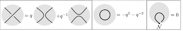
Figure 1. Skein relation, trivial loop relation, trivial arc relation

More precisely,

• The skein relation: if $L,L_{+},L_{-}$ are identical except in a ball in which they look like in Figure 2, then

  $$L=qL_{+}+q^{-1}L_{-}$$

  

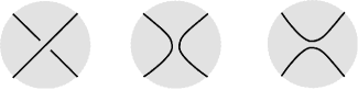
  Figure 2. From left to right: $L,L_{+},L_{-}$.

• The trivial loop relation: If $L$ is a loop bounding a disk in $M$ with framing perpendicular to the disk, then

  $$L=-q^{2}-q^{-2}.$$

• The trivial arc relation: If $L=L^{\prime}\sqcup a$, where $a$ is a trivial arc in $M\setminus L^{\prime}$ then $L=0$. Here $a$ is an trivial arc in $M\setminus L^{\prime}$ means $a$ and a part of $\mathcal{N}$ co-bound an embedded disc in $M\setminus L^{\prime}$.

Proposition 3.1.

In $\mathscr{S}(M,\mathcal{N})$, the reordering relation depicted in Figure 3 holds.

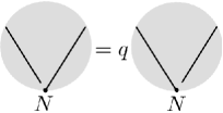
Figure 3. Reordering relation.

Here in Figure 3 we assume that $\mathcal{N}$ is perpendicular to the page and its intersection with the page is the bullet denoted by $N$. The vector of orientation of $\mathcal{N}$ is pointing to the reader. There are two strands of the links coming to $\mathcal{N}$ near $N$, the lower one being depicted by the broken line.

Proof.

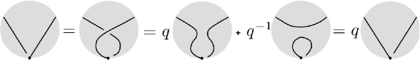
Figure 4. Proof of Proposition 3.1

The proof is given in Figure 4. Here the first identity is an isotopy, the second is the skein relation, the third follows from the trivial arc relation. ∎

Remark 3.2.

(a) The orientation of $M$ is very important in the skein relation.

(b) Kauffman bracket skein modules were introduced by J. Przytycki [Pr] and V. Turaev [Tu] for the case when the marking set $\mathcal{N}$ is empty. Muller [Mu] introduced Kauffman bracket skein modules for marked surfaces, see Section 5. Here we generalize Muller definition to the case of marked 3-manifolds. At first glance, our definition is different from that of Muller for the original case of marked surfaces. The reason is Muller used link diagrams to define the skein modules, and he has to impose the reordering relation since it is not a consequence of other relations if one considers link diagrams. Here we use links in 3-manifolds, and the reordering relation is a consequence of the other relations and the topology afforded by the 3-rd dimension.

4. Generalized marked Surfaces

Here we present basic facts about surfaces, their triangulations, and the vertex matrix and the face matrix associated to a triangulation. In Subsection 4.5 we discuss the duality between the vertex matrix and the face matrix.

4.1. Definitions and basic facts

A generalized marked surface $(\Sigma,\mathcal{P})$ consists of a connected compact oriented surface $\Sigma$ with (possibly empty) boundary $\partial\Sigma$, and a finite set $\mathcal{P}\subset\Sigma$. Elements of $\mathcal{P}$ are called marked points. If $\mathcal{P}\subset\partial\Sigma$, then $(\Sigma,\mathcal{P})$ is called a marked surface.

A $\mathcal{P}$-link in $\Sigma$ is an immersion $\alpha:C\to\Sigma$, where $C$ is compact 1-dimensional non-oriented manifold, such that

• the restriction of $\alpha$ onto the interior of $C$ is an embedding into $\Sigma\setminus\mathcal{P}$, and

• $\alpha$ maps the boundary of $C$ into $\mathcal{P}$.

The image of a connected component of $C$ is called a component of $\alpha$. When $C$ is a $S^{1}$, we call $\alpha$ an $\mathcal{P}$-knot, and when $C$ is $[0,1]$, we call $\alpha$ a $\mathcal{P}$-arc. Two $\mathcal{P}$-links are $\mathcal{P}$-isotopic if they are isotopic in the class of $\mathcal{P}$-links. Very often we identify a $\mathcal{P}$-link with its image in $\Sigma$.

Suppose $\alpha,\beta$ are $\mathcal{P}$-links. An internal common point of $\alpha$ and $\beta$ is point in $(\alpha\cap\beta)\setminus\mathcal{P}$. Let $\mu(\alpha,\beta)$ denote the minimum number of internal common points of $\alpha^{\prime}$ and $\beta^{\prime}$, over all transverse pairs $(\alpha^{\prime},\beta^{\prime})$ such that $\alpha^{\prime}$ is $\mathcal{P}$-isotopic to $\alpha$ and $\beta^{\prime}$ is $\mathcal{P}$-isotopic to $\beta$. It is known that there is a $\mathcal{P}$-link $\gamma$ $\mathcal{P}$-isotopic to $\beta$ such that $|\gamma\cap a|=\mu(\beta,a)$ for any component $a$ of $\alpha$, see [FSH, FST].

A $\mathcal{P}$-link is essential if it does not have a component bounding a disk whose interior is in $\Sigma\setminus\mathcal{P}$; such a component is either a smooth trivial knot in $\Sigma\setminus\mathcal{P}$, or a closed $\mathcal{P}$-arc bounding a disk whose interior is in $\Sigma\setminus\mathcal{P}$. By convention, the empty set is considered an essential $\mathcal{P}$-link.

A $\mathcal{P}$-arc is called a boundary arc if it is $\mathcal{P}$-isotopic to an arc in $\partial\Sigma$. A $\mathcal{P}$-arc is inner if it is not a boundary arc.

4.2. Triangulation

A $\mathcal{P}$-triangulation of $\Sigma$, also called a triangulation of $(\Sigma,\mathcal{P})$, is a triangulation of $\Sigma$ whose set of vertices is $\mathcal{P}$. We will always assume that $(\Sigma,\mathcal{P})$ is triangulable, i.e. it has at least one $\mathcal{P}$-triangulation. It is known that $(\Sigma,\mathcal{P})$ is triangulable if and only if every connected component of $\partial\Sigma$ has at least one marked point and $M$ is not one of the following:

• a sphere with one or two marked points;

• a monogon with no interior marked point; or

• a digon with no interior marked point;

For a triangulable generalized marked surface $(\Sigma,\mathcal{P})$, one can use the following more technical definition (see e.g. [FST, Mu]) of triangulation.

A $\mathcal{P}$-triangulation of $\Sigma$ is a collection $\Delta$ of $\mathcal{P}$-arcs such that

• no two $\mathcal{P}$-arcs in $\Delta$ intersect in $\Sigma\setminus\mathcal{P}$ and no two are $\mathcal{P}$-isotopic, and

• $\Delta$ is maximal amongst all collections of $\mathcal{P}$-arcs with the above property.

An element of $\Delta$ is called an edge of the triangulation. It can be proved that if $\Delta$ is a triangulation, then one can replace $\mathcal{P}$-arcs in $\Delta$ by $\mathcal{P}$-arcs in their respective $\mathcal{P}$-isotopy classes such that every boundary arc in $\Delta$ does lie on the boundary $\partial\Sigma$. We always assume the $\mathcal{P}$-arcs in a triangulation satisfy this requirement.

A triangulated generalized marked surface is a generalized marked surface equipped with a triangulation.

A $\mathcal{P}$-$n$-gon is a smooth map $\gamma:\sigma\to\Sigma$ from a regular $n$-gon $\sigma$ (in the standard plane) to $\Sigma$ such that (a) the restriction of $\gamma$ onto the interior $\mathring{\sigma}$ of $\sigma$ is a diffeomorphism onto its image, (b) the restriction of $\gamma$ onto each edge of $\sigma$ is a $\mathcal{P}$-arc, called an edge of $\gamma$.

A $\mathcal{P}$-triangulation $\Delta$ cuts $\Sigma$ into $\mathcal{P}$-triangles, i.e. the closure of each connected component of $\Sigma\setminus E_{\Delta}$, where $E_{\Delta}=\cup_{a\in\Delta}a$, has the structure of a $\mathcal{P}$-triangle. Denote by $\mathcal{F}(\Delta)$ the set of all triangles of the triangulation $\Delta$. Note that two edges of a triangle $\tau\in\mathcal{F}(\Delta)$ either coincide (i.e. have the same images) or do not have internal common points and are not $\mathcal{P}$-isotopic. When two edges of a triangle $\tau\in\mathcal{F}(\Delta)$ coincide, $\tau$ is called a self-folded triangle, see Figure 5. If $(\Sigma,\mathcal{P})$ is a marked surface, i.e. $\mathcal{P}\subset\partial\Sigma$, then a triangulation of $(\Sigma,\mathcal{P})$ cannot have self-folded triangle.

Figure 5. A triangle and a self-folded triangle

A $\mathcal{P}$-knot is said to be $\Delta$-normal, where $\Delta$ is a $\mathcal{P}$-triangulation, if $\alpha$ is non-trivial and $|\alpha\cap a|=\mu(\alpha,a)$ for all $a\in\Delta$. Every non-trivial $\mathcal{P}$-knot is $\mathcal{P}$-isotopic to a $\Delta$-normal knot.

4.3. Face matrix

Let $\Delta$ be a triangulation of generalized marked surface $(\Sigma,\mathcal{P})$ and $\tau\in\mathcal{F}(\Delta)$, i.e. $\tau$ is a triangle of $\Delta$. We define a anti-symmetric matrix $Q_{\tau}\in\mathrm{Mat}(\Delta\times\Delta,\mathbb{Z})$ as follows. If $\tau$ is a self-folded triangle, then let $Q_{\tau}$ be the 0 matrix. If $\tau$ is not self-folded and hence has 3 distinct edges $a,b,c$ in counterclockwise order (see Figure 5), then define

$$Q_{\tau}(a,b) =Q_{\tau}(b,c)=Q_{\tau}(c,a)=1$$

$$Q_{\tau}(e,e^{\prime}) =0\quad\text{if one of $e,e^{\prime}$ is not in $\{a,b,c\}$ }.$$

In other words, $Q_{\tau}\in\mathrm{Mat}(\Delta\times\Delta,\mathbb{Z})$ is the 0-extension of the following $\{a,b,c\}\times\{a,b,c\}$ matrix

(7) $$\begin{pmatrix}0&1&-1\\ -1&0&1\\ 1&-1&0\end{pmatrix}.$$

Define the face matrix $Q=Q_{\Delta}\in\mathrm{Mat}(\Delta\times\Delta,\mathbb{Z})$ by

$$Q=\sum_{\tau\in\mathcal{F}(\Delta)}Q_{\tau}.$$

Lemma 4.1.

Suppose $\tau\in\mathcal{F}(\Delta)$ has edges $a,b,c$ as in Figure 5 and $\mathbf{k}\in\mathbb{Z}^{\Delta}$. Then

(8) $$(\mathbf{k}Q_{\tau})(c)=\mathbf{k}(b)-\mathbf{k}(a)$$

Proof.

The proof follows immediately from the explicit form (7) of $Q_{\tau}$. ∎

Remark 4.2.

Our $Q$ is the same as $Q^{\Delta}$ of [Mu] or the same as $-B$ of [FST], and is also known as the signed adjacency matrix. We use the terminology “face matrix” to emphasize the duality with the “vertex matrix”.

4.4. Marked surface and its vertex matrix

Assume $(\Sigma,\mathcal{P})$ is a triangulable marked surface. In particular, $\mathcal{P}\subset\partial\Sigma$. Let $\Delta$ be a triangulation of $(\Sigma,\mathcal{P})$.

For each edge $a\in\Delta$ choose an interior point in $a$. Removing this interior point, from $a$ we get two half-edges, each is incident to exactly one vertex in $\mathcal{P}$. Suppose $p\in\mathcal{P}$ and $a^{\prime},b^{\prime}$ are two half-edges (of two different edges) incident to $p$. Define $P_{p}(a^{\prime},b^{\prime})$ as in Figure 6, i.e.

$$P_{p}(a^{\prime},b^{\prime})=\begin{cases}1&\text{if $a^{\prime}$ is clockwise to $b^{\prime}$ (at vertex $p$)}\\ -1&\text{if $a^{\prime}$ is counter-clockwise to $b^{\prime}$ (at vertex $p$)}.\end{cases}$$

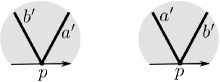
Figure 6. $P_{p}(a^{\prime},b^{\prime})=1$ for the left case, and $P_{p}(a^{\prime},b^{\prime})=-1$ for the right one. Here the shaded area is part of $\Sigma$, and the arrow edge is part of a boundary edge. There might be other half-edges incident to $p$, and they maybe inside and outside the angle between $a^{\prime}$ and $b^{\prime}$

Also, if one of $a^{\prime},b^{\prime}$ is not incident to $p$, set $P_{p}(a^{\prime},b^{\prime})=0$. Define the vertex matrix $P=P(\Delta)\in\mathrm{Mat}(\Delta\times\Delta,\mathbb{Z})$ by

$$P(a,b)=\sum P_{p}(a^{\prime},b^{\prime}),$$

where the sum is over all $p\in\mathcal{P}$, all half-edges $a^{\prime}$ of $a$, and all half-edges $b^{\prime}$ of $b$.

Remark 4.3.

The fact that $\mathcal{P}\subset\partial\Sigma$ is crucial for the definition of the vertex matrix. The vertex matrix were first introduced in [Mu], where it is called the orientation matrix.

4.5. Vertex matrix versus face matrix

The following relation between the face and the vertex matrices of a marked surface is important for us.

Recall that an edge $a\in\Delta$ is a boundary edge if it is a boundary $\mathcal{P}$-arc, otherwise it is called an inner edge. Let ${\mathring{\Delta}}$ be the set of all inner edges. Let ${\mathring{Q}}$ be the $({\mathring{\Delta}}\times{\mathring{\Delta}})$-submatrix of $Q$ and $H$ be the $({\mathring{\Delta}}\times\Delta)$-submatrix of $Q$.

Lemma 4.4.

Suppose $(\Sigma,\mathcal{P})$ is a marked surface with a triangulation $\Delta$.

(a) One has $HPH^{\dagger}=-4{\mathring{Q}}$.

(b) The rank of $H$ is $|{\mathring{\Delta}}|$.

Proof.

(a) Let ${\mathrm{id}}_{\Delta\times{\mathring{\Delta}}}\in\mathrm{Mat}(\Delta\times{\mathring{\Delta}},\mathbb{Z})$ be the matrix which has 1 on the main diagonal, and 0 everywhere else, i.e. ${\mathrm{id}}_{\Delta\times{\mathring{\Delta}}}(a,b)=\delta_{a,b}$. By [Mu, Proposition 7.8],

(9) $$PH^{\dagger}=-4{\mathrm{id}}_{\Delta\times{\mathring{\Delta}}}.$$

Hence $HPH^{\dagger}=-4H\,{\mathrm{id}}_{\Delta\times{\mathring{\Delta}}}=-4{\mathring{Q}}$.

(b) Since $H$ has $|{\mathring{\Delta}}|$ rows, $\mathrm{rk}(H)\leq|{\mathring{\Delta}}|$. Because $\mathrm{rk}({\mathrm{id}}_{\Delta\times{\mathring{\Delta}}})=|{\mathring{\Delta}}|$, Equation (9) shows that $\mathrm{rk}(H)\geq|{\mathring{\Delta}}|$. Hence $\mathrm{rk}(H)=|{\mathring{\Delta}}|$. ∎

5. Skein algebra of marked surfaces

Throughout this section we fix a marked surface $(\Sigma,\mathcal{P})$.

5.1. Skein module of marked surface

Let $M$ be the cylinder over $\Sigma$ and $\mathcal{N}$ the cylinder over $\mathcal{P}$, i.e. $M=\Sigma\times(-1,1)$ and $\mathcal{N}=\mathcal{P}\times(-1,1)$. We consider $(M,\mathcal{N})$ as a marked 3-manifold, where the orientation on each component of $\mathcal{N}$ is given by the natural orientation of $(-1,1)$. We identify $\Sigma$ with $\Sigma\times\{0\}\subset M$. There is a vertical projection $\operatorname{pr}:M\to\Sigma$, mapping $(z,t)$ to $z$. The number $t$ is called the height of $(z,t)$. The vertical vector at $(z,t)\in\Sigma\times(-1,1)$ is the unit vector tangent to $z\times(-1,1)$ and having direction the positive orientation of $(-1,1)$.

Define $\mathscr{S}(\Sigma,\mathcal{P}):=\mathscr{S}(M,\mathcal{N})$. Since we fix $(\Sigma,\mathcal{P})$, we will denote $\mathscr{S}$ for $\mathscr{S}(\Sigma,\mathcal{P})$ in this section.

Suppose $\alpha\subset\Sigma$ is a $\mathcal{P}$-link. We will define $[\alpha]\in\mathscr{S}$ as follows. Let $\alpha^{\prime}\subset\Sigma\times(-1,1)$ be an $\mathcal{N}$-link such that

• $\operatorname{pr}(\alpha^{\prime})=\alpha$, the framing of $\alpha^{\prime}$ is vertical everywhere, and

• for every $p\in\mathcal{P}$, if $a_{1},\dots,a_{k_{p}}$ are strands of $\alpha$ (in a small neighborhood of $p$) coming to $p$ in clockwise order, and $a_{1}^{\prime},\dots,a^{\prime}_{k_{p}}$ are the strands of $\alpha^{\prime}$ projecting correspondingly onto $a_{1},\dots,a_{k_{p}}$, then the height of $a_{i}^{\prime}$ is greater than that of $a^{\prime}_{i+1}$ for $i=1,\dots,k_{p}-1$. See an example with $k_{p}=3$ in Figure 7.

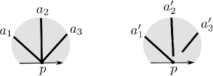
Figure 7. Left: There are 3 strands $a_{1},a_{2},a_{3}$ of $\alpha$ coming to $p$, ordered clockwise. Right: The corresponding strands $a^{\prime}_{1},a^{\prime}_{2},a^{\prime}_{3}$ of $\alpha^{\prime}$, with $a^{\prime}_{1}$ above $a^{\prime}_{2}$, and $a^{\prime}_{2}$ above $a^{\prime}_{3}$.

It is clear that the $\mathcal{N}$-isotopy class of $\alpha^{\prime}$ is determined by $\alpha$. Define $\alpha$ as an element in $\mathscr{S}$ by

(10) $$[\alpha]=q^{\frac{1}{4}\sum_{p\in\mathcal{P}}(k_{p}-1)(k_{p}-2)}\alpha^{\prime}.$$

The factor which is a power of $q$ on the right hand side is introduced so that $[\alpha]$ is invariant under a certain transformation, see Section 5.2. By [Mu, Lemma 4.1], we have the following fact, which had been known for unmarked surface [PS].

Proposition 5.1 ([Mu]).

As an ${\mathcal{R}}$-module, $\mathscr{S}$ is a free with basis the set of all $[\alpha]$, where $\alpha$ runs the set of all $\mathcal{P}$-isotopy classes of essential $\mathcal{P}$-links.

A concise and simple proof of this fact can be obtained using the Diamond Lemma as in [SW]. We will consider $\mathscr{S}$ as a based ${\mathcal{R}}$-module with the preferred base described by Proposition 5.1. In what follows we often use the same notation, say $\alpha$, to denote a $\mathcal{P}$-link and the element $[\alpha]$ of $\mathscr{S}$ when there is no confusion.

5.2. Algebra structure and reflection anti-involution

For $\mathcal{N}$-links $\alpha_{1},\alpha_{2}$ in $M=\Sigma\times(-1,1)$, considered as elements of $\mathscr{S}$, define the product $\alpha_{1}\alpha_{2}$ as the result of stacking $\alpha_{1}$ atop $\alpha_{2}$ using the cylinder structure of $(M,\mathcal{N})$. Precisely this means the following. Let $\iota_{1}:\Sigma\times(-1,1)\hookrightarrow\Sigma\times(-1,1)$ be the embedding $\iota_{1}(x,t)=(x,\frac{t+1}{2})$ and $\iota_{2}:\Sigma\times(-1,1)\hookrightarrow\Sigma\times(-1,1)$ be the embedding $\iota_{1}(x,t)=(x,\frac{t-1}{2})$. Then $\alpha_{1}\alpha_{2}:=\iota_{1}(\alpha_{1})\cup\iota_{2}(\alpha_{2})$. This product makes $\mathscr{S}$ an ${\mathcal{R}}$-algebra, which is non-commutative in general.

Let $\chi:\mathscr{S}\to\mathscr{S}$ be the bar homomorphism of [Mu], which is the $\mathbb{Z}$-algebra anti-homomorphism defined by (i) $\chi(q^{1/8})=q^{-1/8}$ and (ii) $\chi(L)$ is the reflection image of $L$ for any $\mathcal{N}$-link $L$ in $\Sigma\times(-1,1)$. Here the reflection is the map $(z,t)\to(z,-t)$ of $\Sigma\times(-1,1)$. It is clear that $\chi$ is an anti-involution. An element $\alpha\in\mathscr{S}(\Sigma,\mathcal{P})$ is reflection invariant if $\chi(\alpha)=\alpha$. From the reordering relation (Proposition 3.1) one can easily show that $[\alpha]$ is reflection-invariant for any $\mathcal{P}$-link $\alpha$.

5.3. Functoriality

Let $(\Sigma^{\prime},\mathcal{P}^{\prime})$ be a marked surface such that $\Sigma^{\prime}\subset\Sigma$ and $\mathcal{P}^{\prime}\subset\mathcal{P}$. The embedding $\iota:\Sigma^{\prime}\hookrightarrow\Sigma$ induces an ${\mathcal{R}}$-algebra homomorphism $\iota_{*}:\mathscr{S}(\Sigma^{\prime},\mathcal{P}^{\prime})\to\mathscr{S}(\Sigma,\mathcal{P})$.

If $\Sigma^{\prime}=\Sigma$, then $\iota_{*}:\mathscr{S}(\Sigma,\mathcal{P}^{\prime})\to\mathscr{S}(\Sigma,\mathcal{P})$ is injective, because the preferred basis of $\mathscr{S}(\Sigma,\mathcal{P}^{\prime})$ is a subset of that of $\mathscr{S}(\Sigma,\mathcal{P})$.

In particular, the natural ${\mathcal{R}}$-algebra homomorphism $\iota_{*}:\mathring{\mathscr{S}}\to\mathscr{S}$ is injective, where $\mathring{\mathscr{S}}=\mathscr{S}(\Sigma,\emptyset)$. We will always identify $\mathring{\mathscr{S}}$ with a subset of $\mathscr{S}$ via $\iota_{*}$.

5.4. Muller’s algebra: quantum torus associated to vertex matrix

Suppose $(\Sigma,\mathcal{P})$ has a triangulation $\Delta$. By definition, each $a\in\Delta$ is an $\mathcal{N}$-arc (with vertical framing), and we consider $a$ as an element of the skein algebra $\mathscr{S}$. From the reordering relation (Proposition 3.1) we see that for each pair $a,b\in\Delta$ one has

(11) $$ab=q^{P(a,b)}ba,$$

where $P\in\mathrm{Mat}(\Delta\times\Delta,\mathbb{Z})$ is the vertex matrix (see Subsection 4.4). It is the $q$-commutativity of edges of $\Delta$, equation (11), that leads to the introduction of the vertex matrix in [Mu].

The Muller algebra $\mathfrak{X}(\Delta)$ is defined to be the quantum torus $\mathbb{T}(P,q,X)$, i.e.

$$\mathfrak{X}(\Delta)={\mathcal{R}}\langle X_{a}^{\pm 1},a\in\Delta\rangle/(X_{a}X_{b}=q^{P(a,b)}X_{b}X_{a}).$$

Denote by $\tilde{\mathfrak{X}}(\Delta)$ the skew field of $\mathfrak{X}(\Delta)$. Recall that $\mathfrak{X}(\Delta)$ is a based ${\mathcal{R}}$-module with preferred basis $\{X^{\mathbf{k}}\mid\mathbf{k}\in\mathbb{Z}^{\Delta}\}$. Let $\mathfrak{X}_{++}(\Delta)$ be the ${\mathcal{R}}$-submodule of $\mathfrak{X}(\Delta)$ spanned by $X^{\mathbf{k}}$ with $\mathbf{k}\in\mathbb{N}^{\Delta}$, i.e. $\mathbf{k}(a)\geq 0$ for all $a\in\Delta$. Then $\mathfrak{X}_{++}(\Delta)$ is an ${\mathcal{R}}$-subalgebra of $\mathfrak{X}(\Delta)$.

Relation (11) shows that there is a unique algebra homomorphism

(12) $$\phi_{\Delta}:\mathfrak{X}_{++}(\Delta)\to\mathscr{S},\quad\text{defined by $\phi_{\Delta}(a)=X_{a}$}.$$

For $\mathbf{k}\in\mathbb{N}^{\Delta}$, the image $\Delta^{\mathbf{k}}:=\phi_{\Delta}(X^{\mathbf{k}})$ has a transparent geometric description. In fact, as observed in [Mu], $\Delta^{\mathbf{k}}$ is a $\mathcal{P}$-link consisting of $\mathbf{k}(a)$ copies of $a$ for every $a\in\Delta$. Here each copy of $a$, by definition, is a $\mathcal{P}$-arc $\mathcal{P}$-isotopic to $a$ in $\Sigma\setminus\left(\cup_{b\in\Delta\setminus\{a\}}b\right)$. This gives a nice geometric interpretation of the Weyl normalization.

The following is one of the main results of [Mu].

Theorem 5.2 (Muller).

(i) The homomorphism $\phi_{\Delta}$ in (12) is injective.

(ii) There is a unique injective algebra homomorphism $\varphi_{\Delta}:\mathscr{S}\hookrightarrow\mathfrak{X}(\Delta)$ such that $\varphi_{\Delta}\circ\phi_{\Delta}$ is the identity on $\mathfrak{X}_{++}(\Delta)$. In other words, the combination

(13) $$\mathfrak{X}_{++}(\Delta)\overset{\phi_{\Delta}}{\lhook\joinrel\relbar\joinrel\rightarrow}\mathscr{S}\overset{\varphi_{\Delta}}{\lhook\joinrel\relbar\joinrel\rightarrow}\mathfrak{X}(\Delta)$$

is the natural embedding $\mathfrak{X}_{++}(\Delta)\hookrightarrow\mathfrak{X}(\Delta)$. Besides, $\varphi_{\Delta}$ is reflection invariant, i.e. $\varphi_{\Delta}$ commutes with $\chi$.

We will call $\varphi_{\Delta}$ the skein coordinate map of $\mathscr{S}$ associated to the triangulation $\Delta$. The skein coordinates, in the classical case $q=1$, correspond to the Penner coordinates on decorated Teichmüller spaces [Pe]. We will identify $\mathscr{S}$ with a subset of $\mathfrak{X}(\Delta)$ via the embedding $\varphi_{\Delta}$. Then $\mathscr{S}$ is sandwiched between $\mathfrak{X}_{++}(\Delta)$ and $\mathfrak{X}(\Delta)$.

While $\mathscr{S}$ is a complicated algebra, $\mathfrak{X}(\Delta)$ has a simple algebraic structure. Being a subring of a two-sided Noetherian domain $\mathfrak{X}(\Delta)$, $\mathscr{S}$ is a two-sided Noetherian domain, and hence a two-sided Ore domain, see [GW]. It follows that the skew field $\tilde{\mathscr{S}}$ of $\mathscr{S}$ exists. The inclusions in (13) shows that $\tilde{\mathfrak{X}}(\Delta)=\tilde{\mathscr{S}}$. The inclusions in (13) also show that $\mathscr{S}$ is an essential subalgebra of $\mathfrak{X}(\Delta)$ in the sense that every algebra homomophism from $\mathfrak{X}(\Delta)$ to another algebra is totally determined by it restriction on $\mathscr{S}$.

Let $\mathfrak{X}^{(\frac{1}{2})}(\Delta)$ be the quantum torus $\mathbb{T}(P,q^{1/4},x)$, which has basis variables $x_{a},a\in\Delta$. We consider $\mathfrak{X}(\Delta)$ as a ${\mathcal{R}}$-subalgebra of $\mathfrak{X}^{(\frac{1}{2})}(\Delta)$ by setting $X_{a}=(x_{a})^{2}$.

Remark 5.3.

In [Le2] we extend Theorem 5.2 to the case when the marked surfaces have interior marked points (or punctures), or some of boundary components of $\Sigma$ do not have marked points. The advantage of having boundary components without marked points is that we can build a surgery theory, and can alter the topology of the surfaces.

5.5. Flips of triangulations

Let us recall the flip of a triangulation at an inner edge. Suppose $\Delta$ is a triangulation of $(\Sigma,\mathcal{P})$ and $a$ is an inner edge of $\Delta$. There is a unique (up to $\mathcal{P}$-isotopy) $\mathcal{P}$-arc $a^{*}$ different from $a$ such that $\Delta^{\prime}=\Delta\setminus\{a\}\cup\{a^{*}\}$ is a triangulation, and we call $\Delta^{\prime}$ the flip of $\Delta$ at $a$.

Figure 8. Flip at $a$.

One can obtain $a^{*}$ is as follows. The two triangles, each having $a$ as an edge, together form a $\mathcal{P}$-quadrilateral, with $a$ being one of its two diagonals, see Figure 8. Then $a^{*}$ is the other diagonal. The edges $b,c,d,e$ in Figure 8 are not necessarily pairwise distinct. If they are not, then either $b=d$ or $c=e$ (but not both) as all other cases are excluded because $\mathcal{P}\subset\partial\Sigma$.

It is known that for any two triangulations are related by a sequence of flips [FST].

5.6. Coordinate change

Suppose $\Delta,\Delta^{\prime}$ are two triangulations of $(\Sigma,\mathcal{P})$. We have the following algebra isomorphisms (skein coordinate maps)

$$\varphi_{\Delta}:\tilde{\mathscr{S}}\overset{\cong}{\longrightarrow}\tilde{\mathfrak{X}}(\Delta),\quad\varphi_{\Delta^{\prime}}:\tilde{\mathscr{S}}\overset{\cong}{\longrightarrow}\tilde{\mathfrak{X}}(\Delta^{\prime}).$$

The coordinate change map $\Phi_{\Delta,\Delta^{\prime}}:\tilde{\mathfrak{X}}(\Delta^{\prime})\to\tilde{\mathfrak{X}}(\Delta)$ is defined by $\Phi_{\Delta,\Delta^{\prime}}:=\varphi_{\Delta}\circ(\varphi_{\Delta^{\prime}})^{-1}$, which is an ${\mathcal{R}}$-algebra isomorphism.

Proposition 5.4.

(a) The coordinate change isomorphism $\Phi_{\Delta,\Delta^{\prime}}$ is natural. This means,

$$\Phi_{\Delta,\Delta}=\mathrm{Id},\quad\Phi_{\Delta,\Delta^{\prime\prime}}=\Phi_{\Delta,\Delta^{\prime}}\circ\Phi_{\Delta^{\prime},\Delta^{\prime\prime}}.$$

(b) The maps $\varphi_{\Delta}:\mathscr{S}\hookrightarrow\tilde{\mathfrak{X}}(\Delta)$ commute with the coordinate change maps, i.e.

$$\varphi_{\Delta}=\Phi_{\Delta,\Delta^{\prime}}\circ\varphi_{\Delta^{\prime}}.$$

(c) Suppose $\Delta^{\prime}$ is obtained from $\Delta$ by a flip at an edge $a$, with $a$ replaced by $a^{*}$ as in Figure 8. Then $\Phi_{\Delta\Delta^{\prime}}(X_{v})=X_{v}$ for any $v\in\Delta\setminus\{a^{*}\}$ and, with notations of edges as in Figure 8,

(14) $$\Phi_{\Delta\Delta^{\prime}}(X_{a*})=[X_{c}X_{e}X_{a}^{-1}]+[X_{b}X_{d}X_{a}^{-1}].$$

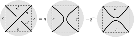
Figure 9. Proof of (15)

Proof.

Parts (a) and (b) follow right away from the definition. Let us prove (c). It is clear that $\Phi_{\Delta\Delta^{\prime}}(X_{v})=X_{v}$ for any $v\in\Delta\setminus\{a^{*}\}$. In $\mathscr{S}$, using the skein relation (see Figure 9), we have

$$aa^{*}=qce+q^{-1}bd.$$

Multiplying $a^{-1}$ on the left,

(15) $$a^{*}=q^{\varepsilon_{1}}[cea^{-1}]+q^{\varepsilon_{2}}[bda^{-1}],$$

where $\varepsilon_{1},\varepsilon_{2}\in\mathbb{Z}$. A careful calculation of $\varepsilon_{1}$ and $\varepsilon_{2}$ using the commutations between $a,b,c,d,e$ will show that $\varepsilon_{1}=\varepsilon_{2}=0$, and we get (14). Another way to show $\varepsilon_{1}=\varepsilon_{2}=0$ is the following. The two monomials $[cea^{-1}]$ and $[bda^{-1}]$ are distinct. In fact, if they are the same, then either $c=b$ or $c=d$, which is impossible because then either $\Delta$ or $\Delta^{\prime}$ has a self-folded triangle. By Lemma 2.3, $\varepsilon_{1}=\varepsilon_{2}=0$. ∎

Remark 5.5.

One advantage of $\mathfrak{X}(\Delta)$ over the Chekhov-Fock algebra (see Section 6) is the coordinate change maps come along naturally and are easy to study.

5.7. Image of $\Delta$-simple knots under $\varphi_{\Delta}$

Suppose $\Delta$ is a triangulation of $(\Sigma,\mathcal{P})$ and $\alpha$ is a $\mathcal{P}$-arc or $\mathcal{P}$-knot. We say that $\alpha$ is $\Delta$-simple if $\mu(\alpha,a)\leq 1$ for all $a\in\Delta$.

Suppose $\alpha$ is a $\Delta$-simple. After an isotopy we can assume that $\alpha$ is $\Delta$-normal, i.e. $\mu(\alpha,a)$ is equal to the number of internal common points of $\alpha$ and $a$, for all $a\in\Delta$. Let $\mathcal{E}(\alpha,\Delta)$ be the set of all edges $e$ in $\Delta$ such that $\mu(\alpha,e)\neq 0$ , and $\mathcal{F}(\alpha,\Delta)$ be the set of all triangles $\tau$ of $\Delta$ intersecting the interior of $\alpha$. It is clear that $\mathcal{E}(\alpha,\Delta)\subset{\mathring{\Delta}}$.

Figure 10. Non-admissible case: $C(a)=-1,C(b)=1$.

A coloring of $(\alpha,\Delta)$ is a map $C\in\mathbb{Z}^{\mathring{\Delta}}$ such that $C(e)=0$ if $e\not\in\mathcal{E}(\alpha,\Delta)$ and $C(e)\in\{1,-1\}$ if $e\in\mathcal{E}(\alpha,\Delta)$. A coloring $C$ of $(\alpha,\Delta)$ is said to be admissible if for any triangle $\tau\in\mathcal{F}(\alpha,\Delta)$ intersecting $\alpha$ at two edges $a$ and $b$, with notations of edges as in Figure 10, one has $(C(a),C(b))\neq(-1,1).$ Denote by $\mathrm{Col}(\alpha,\Delta)$ the set of all admissible colorings of $\alpha$.

Theorem 5.6.

Suppose $\Delta$ is a triangulation of a marked surface $(\Sigma,\mathcal{P})$ and $\alpha$ is a $\Delta$-simple, $\Delta$-normal knot. Then for any $C\in\mathrm{Col}(\alpha,\Delta)$, $CH$ has even entries, and

(16) $$\varphi_{\Delta}(\alpha)=\sum_{C\in\mathrm{Col}(\alpha,\Delta)}x^{CH}.$$

Recall that $H$ is the ${\mathring{\Delta}}\times\Delta$ submatrix of the face matrix $Q=Q_{\Delta}$, and $CH$ is the matrix product where $C$ is considered as a row vector, and $x^{CH}\in\mathfrak{X}^{(\frac{1}{2})}(\Delta)$ is the normalized monomial.

Proof.

To simplify notations we identify $\mathscr{S}$ with its image under the embedding $\varphi_{\Delta}:\mathscr{S}\hookrightarrow\mathfrak{X}(\Delta)$. Thus, for $a\in\Delta$, we have $a=X_{a}=x_{a}^{2}$.

Step 1. Let $E=\bigcup_{e\in\mathcal{E}(\alpha,\Delta)}e$, which is a $\mathcal{P}$-link and will be considered as an element of $\mathscr{S}\subset\mathfrak{X}(\Delta)$. We express explicitly the product $\alpha E$ as a sum of monomials as follows.

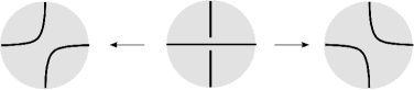
Figure 11. Smoothing of crossing, $+1$ on the left, $-1$ on the right

Each $e\in\mathcal{E}(\alpha,\Delta)$ intersects $\alpha$ at exactly one point. Let $L$ be the $\mathcal{P}$-link diagram $\alpha\cup E,$ with $\alpha$ above all the $e\in\mathcal{E}(\alpha,\Delta)$. Then $L$ represents the product $\alpha E,$ which can be calculated by resolving all the crossings of $L$ using the skein relation. Each crossing of $L$ has two smoothings, the $+1$ one and the $-1$ one, see Figure 11. Each coloring $C$ of $(\alpha,\Delta)$ corresponds to exactly one smoothing of all the crossings of $L$ by the rule: the smoothing of the crossing on the edge $e$ is of type $C(e)$. Let $L_{C}$ be the result of smoothing all the crossings of $L$ according to $C$. Then, with $\|C\|=\sum_{e}C(e)$,

$$\alpha E=\sum_{C}q^{\|C\|}L_{C},$$

where the sum is over all colorings $C$ of $(\alpha,\Delta)$. This implies

(17) $$\alpha=\sum_{C}\alpha_{C},\quad\text{where }\ \alpha_{C}=q^{\|C\|}L_{C}\,E^{-1}$$

Step 2. Note that $L_{C}$ is a collection of $\mathcal{P}$-arcs, with exactly one in each triangle $\tau\in\mathcal{F}(\alpha,\Delta)$, see Figure 12.

Figure 12. Four resolutions of left box corresponding to $(C(a),C(b))=(-1,1)$, $(1,-1)$, $(-1,-1)$, and $(1,1)$

Denote the $\mathcal{P}$-arc of $L_{C}$ in $\tau$ by $\tilde{w}(\alpha,\tau,C)$, which is described in Figure 12:

(18) $$\tilde{w}(\alpha,\tau,C)=\begin{cases}0\quad&\text{if }C(a)=-1,C(b)=1\\ c&\text{if }C(a)=1,C(b)=-1\\ b&\text{if }C(a)=-1,C(b)=-1\\ a&\text{if }C(a)=1,C(b)=1.\end{cases}$$

The first identity of (18) shows that $L_{C}=0$ if $C$ is not admissible. Hence (17) becomes

(19) $$\alpha=\sum_{C\in\mathrm{Col}(\alpha,\Delta)}\alpha_{C},\quad\text{with }\ \alpha_{C}\overset{\bullet}{=}L_{C}\,E^{-1},$$

where $u\overset{\bullet}{=}v$ means $u=q^{r}v$ for some $r\in\mathbb{Q}$. By construction,

(20) $$L_{C}\overset{\bullet}{=}\prod_{\tau\in\mathcal{F}(\alpha,\Delta)}\tilde{w}(\alpha,\tau,C).$$

Step 3. For each $\tau\in\mathcal{F}(\alpha,\Delta)$ with notations of edges as in Figure 10 let

(21) $$E_{\tau}:=x_{a}x_{b}.$$

Since $a=x_{a}^{2}$ and each $\tau\in\mathcal{F}(\alpha,\Delta)$ has two edges intersecting $\alpha$, we have

(22) $$E\overset{\bullet}{=}\prod_{e\in\mathcal{E}(\alpha,\Delta)}e\overset{\bullet}{=}\prod_{e\in\mathcal{E}(\alpha,\Delta)}(x_{e})^{2}\overset{\bullet}{=}\prod_{\tau\in\mathcal{F}(\alpha,\Delta)}E_{\tau}.$$

Using (19), (20), and (22), we have

(23) $$\alpha_{C}\overset{\bullet}{=}L_{C}\,E^{-1}\overset{\bullet}{=}\prod_{\tau\in\mathcal{F}(\alpha,\Delta)}\tilde{w}(\alpha,\tau,C)\,E_{\tau}^{-1}.$$

Step 4. Let $\hat{C}\in\mathbb{Z}^{\Delta}$ be the zero extension of $C\in\mathbb{Z}^{{\mathring{\Delta}}}$. Then $\hat{C}Q=CH$. Using the explicit formula (7) of $Q_{\tau}$ and (18), (21), one can verify that

$$\tilde{w}(\alpha,\tau,C)\,E_{\tau}^{-1}\overset{\bullet}{=}x^{\hat{C}Q_{\tau}}.$$

Hence, (23) implies

(24) $$\alpha_{C}\overset{\bullet}{=}\prod_{\tau\in\mathcal{F}(\alpha,\Delta)}x^{\hat{C}Q_{\tau}}\overset{\bullet}{=}x^{\hat{C}Q}=x^{CH}.$$

Step 5. From (19) and (24), we have

$$\alpha=\sum_{C\in\mathrm{Col}(\alpha,\Delta)}q^{f(C)}x^{CH},$$

with $f_{C}\in\mathbb{Q}$. Since $\mathrm{rk}(H)=|{\mathring{\Delta}}|$ (by Lemma 4.4), $CH$ are distinct when $C$ runs the set $\mathrm{Col}(\alpha,\Delta)$. Because $\alpha$ is reflection invariant, Lemma 2.3 shows that $f_{C}=0$ for all $C\in\mathrm{Col}(\alpha,\Delta)$. This proves (16), as equality in $\mathfrak{X}^{(\frac{1}{2})}(\Delta)$.

Step 6. Equation (16) and Lemma 2.5 shows that each $x^{CH}$ is in $\mathfrak{X}(\Delta)$, which is equivalent to $CH$ has even entries. This completes the proof of the theorem. ∎

Remark 5.7.

The fact that $CH$ has even entries can be proved directly easily. A more general fact is proved in Lemma 6.2 below.

5.8. Triangulation-simple knots

Theorem 5.6 gives the image under $\varphi_{\Delta}$ of $\Delta$-simple knots, but not all $\mathring{\mathscr{S}}=\mathscr{S}(\Sigma,\emptyset)$. Following is the reason why in many applications this should be enough.

A knot $\alpha\in\Sigma$ is triangulation-simple if there is a triangulation $\Delta$ such that $\alpha$ is $\Delta$-simple.

Proposition 5.8.

Suppose $(\Sigma,\mathcal{P})$ is a triangulable marked surface. Then the algebra $\mathring{\mathscr{S}}$ is generated by the set of all triangulation-simple knots.

Proof.

Let $\Delta$ be a triangulation of $(\Sigma,\mathcal{P})$ and $\Gamma\subset{\mathring{\Delta}}$ be a maximal subset such that by splitting $\Sigma$ along edges in $\Gamma$ one gets a disk. The resulting disk, denoted by $\bar{\Sigma}$, inherits a triangulation ${\bar{\Delta}}$ from $\Delta$. According to [Mu, Appendix A] ( see also [Bu2]), $\mathring{\mathscr{S}}$ is generated by knots in $\mathring{\Sigma}$ which meet each edge in $\Gamma$ at most once. Such a knot $\alpha$, when cut by $\Gamma$, is a collection of non-intersecting intervals, called $\alpha$-intervals, in the polygon $\bar{\Sigma}$. Each $\alpha$-interval has end points on boundary edges of ${\bar{\Delta}}$, called the ending edges of the interval. No two different intervals have a common ending edge. After an isotopy we can assume that the edges of ${\bar{\Delta}}$ and all $\alpha$-intervals are straight lines on the plane. For an $\alpha$-interval, the convex hull of its ending edges is either a triangle (when the two ending edges have a common vertex) or a quadrilateral, called the hull of the interval. The hulls of two different $\alpha$-intervals do not have interior intersection. For each hull which is a quadrilateral choose a triangulation of it by adding one of its diagonals. Let $\Delta^{\prime}$ be any triangulation of $\Sigma$ extending the triangulations of all of the hulls. Then $\alpha$ is $\Delta^{\prime}$-simple. This proves the proposition. ∎

5.9. Image of $\Delta$-simple arcs

Suppose $\alpha$ is a $\Delta$ simple, $\Delta$-normal $\mathcal{P}$-arc. We assume $\alpha\not\in\Delta$.

Figure 13. A $\Delta$-simple arc $\alpha$. One might have $p_{1}=p_{2}$, and one of $a_{1}^{\prime},a_{1}^{\prime\prime}$ might be one of $a_{2}^{\prime},a_{2}^{\prime\prime}$

Then, with notations of edges as in Figure 13, one has

(25) $$\alpha=\sum_{C\in\mathrm{Col}(\alpha,\Delta)}\left[x^{CQ}\,x_{a^{\prime}_{1}}x_{a^{\prime\prime}_{1}}(x_{a_{1}})^{-1}\,x_{a^{\prime}_{2}}x_{a^{\prime\prime}_{2}}(x_{a_{2}})^{-1}\right]$$

The proof is a simple modification of that of Theorem 5.6, taking into account what happens near the end points of $\alpha$, and is left for the dedicated reader. We will not need this result in the current paper.

6. Chekhov-Fock algebra of marked surfaces and shear coordinates

In this section we show how the quantum trace map of Bonahon and Wong can be recovered from the natural embedding $\varphi_{\Delta}:\mathscr{S}(\Sigma,\emptyset)\hookrightarrow\mathfrak{X}(\Delta)$ by the shear-to-skein map and give an intrinsic description of the quantum Teichmüller space, for the case when $(\Sigma,\mathcal{P})$ is a triangulated marked surface.

Throughout this section we fix a triangulable marked surface $(\Sigma,\mathcal{P})$; $\Delta$ will be a triangulation of $(\Sigma,\mathcal{P})$. We use notations $\mathring{\mathscr{S}}=\mathscr{S}(\Sigma,\emptyset)$ and $\mathscr{S}=\mathscr{S}(\Sigma,\mathcal{P})$.

6.1. Chekhov-Fock algebra and its square root version

Here we define the Chekhov-Fock algebra $\mathcal{Y}^{(2)}(\Delta)$ and its square root version $\mathcal{Y}^{\mathrm{bl}}(\Delta)$ mentioned in Introduction.

In this subsection we allow $(\Sigma,\mathcal{P})$ to be more general, namely $(\Sigma,\mathcal{P})$ is a triangulated generalized marked surface, with triangulation $\Delta$. The face matrix $Q=Q_{\Delta}\in\mathrm{Mat}(\Delta\times\Delta,\mathbb{Z})$ is defined (see Section 4.3), but the vertex matrix $P$ cannot not be defined if there are interior marked points.

Recall that ${\mathring{Q}}$ is the ${\mathring{\Delta}}\times{\mathring{\Delta}}$ sub matrix of the face matrix $Q=Q_{\Delta}$. Let $\mathcal{Y}(\Delta)$ be the quantum torus $\mathbb{T}({\mathring{Q}},q^{-1},y)$, i.e.

$$\mathcal{Y}(\Delta)=R\langle y_{a}^{\pm 1},a\in{\mathring{\Delta}}\rangle/(y_{a}y_{b}=q^{-{\mathring{Q}}(a,b)}y_{b}y_{a}).$$

Let $Y_{a}=y_{a}^{2}$, for $a\in{\mathring{\Delta}}$. Then the subalgebra $\mathcal{Y}^{(2)}(\Delta)\subset\mathcal{Y}(\Delta)$ generated by $Y_{a}^{\pm 1}$ is the quantum torus $\mathbb{T}({\mathring{Q}},q^{-4},Y)$ with basis variables $Y_{a},a\in{\mathring{\Delta}}$. Let $\tilde{\mathcal{Y}}^{(2)}(\Delta)$ and $\tilde{\mathcal{Y}}(\Delta)$ be respectively the skew fields of $\mathcal{Y}^{(2)}(\Delta)$ and $\mathcal{Y}(\Delta)$. The preferred bases of $\mathcal{Y}(\Delta)$ and $\mathcal{Y}^{(2)}(\Delta)$ are respectively $\{y^{\mathbf{k}}\mid\mathbf{k}\in\mathbb{Z}^{{\mathring{\Delta}}}\}$ and $\{y^{\mathbf{k}}\mid\mathbf{k}\in(2\mathbb{Z})^{{\mathring{\Delta}}}\}$.

An element $\mathbf{k}\in\mathbb{Z}^{\mathring{\Delta}}$ is called $\Delta$-balanced if $\mathbf{k}(\tau)$ is even for any triangle $\tau\in\mathcal{F}(\Delta)$. Here $\mathbf{k}(\tau)=\mathbf{k}(a)+\mathbf{k}(b)+\mathbf{k}(c)$, where $a,b,c$ are edges of $\tau$, with the understanding that $\mathbf{k}(e)=0$ for any boundary edge $e$. Let $\mathcal{Y}^{\mathrm{bl}}(\Delta)$ be the ${\mathcal{R}}$-submodule of $\mathcal{Y}(\Delta)$ spanned by $y^{\mathbf{k}}$ with balanced $\mathbf{k}$. Clearly $\mathcal{Y}^{\mathrm{bl}}(\Delta)$ is an ${\mathcal{R}}$-subalgebra of $\mathcal{Y}(\Delta)$ and $\mathcal{Y}^{(2)}(\Delta)\subset\mathcal{Y}^{\mathrm{bl}}(\Delta)$.

For a $\mathcal{P}$-knot $\alpha$, let $\mathbf{k}_{\alpha}\in\mathbb{Z}^{\Delta}$ be defined by $\mathbf{k}_{\alpha}(e)=\mu(\alpha,e)$, which is clearly $\Delta$-balanced. Recall that $\alpha$ is $\Delta$-simple if $\mathbf{k}_{\alpha}(e)\leq 1$ for all $e\in\Delta$.

Lemma 6.1.

As an ${\mathcal{R}}$-algebra, $\mathcal{Y}^{\mathrm{bl}}(\Delta)$ is generated by $\mathcal{Y}^{(2)}(\Delta)$ and $y^{\mathbf{k}_{\alpha}}$, with all $\Delta$-simple knots $\alpha$.

Proof.

A version of this statement already appeared in [BW1], and we use same proof. Every $\mathbf{k}\in\mathbb{Z}^{\mathring{\Delta}}$ has a unique presentation $\mathbf{k}={\mathbf{u}}+{\mathbf{m}}$ where ${\mathbf{m}}\in(2\mathbb{Z})^{{\mathring{\Delta}}}$ and ${\mathbf{u}}\in\{0,1\}^{\mathring{\Delta}}$. Hence,

$$\mathcal{Y}(\Delta) =\bigoplus_{{\mathbf{u}}\in\{0,1\}^{\mathring{\Delta}}}y^{\mathbf{u}}\mathcal{Y}^{(2)}(\Delta)$$

(26) $$\mathcal{Y}^{\mathrm{bl}}(\Delta) =\bigoplus_{{\mathbf{u}}\in(\{0,1\}^{\mathring{\Delta}})_{\mathrm{bl}}}y^{\mathbf{u}}\mathcal{Y}^{(2)}(\Delta),$$

where $(\{0,1\}^{\mathring{\Delta}})_{\mathrm{bl}}$ is the set of $\Delta$-balanced ${\mathbf{u}}\in\{0,1\}^{\mathring{\Delta}}$. Note that $(\{0,1\}^{\mathring{\Delta}})_{\mathrm{bl}}$ is naturally isomorphic to the homology group $H^{1}(\Sigma,\mathbb{Z}/2)$. For every ${\mathbf{u}}\in(\{0,1\}^{\mathring{\Delta}})_{\mathrm{bl}}$, there exists $\alpha=\sqcup_{i=1}^{j}\alpha_{i}$ such that each $\alpha_{i}$ is a $\Delta$-simple knot and ${\mathbf{u}}=\sum\mathbf{k}_{\alpha_{i}}$. Hence, (26) shows that $\mathcal{Y}^{\mathrm{bl}}(\Delta)$ is generated by $\mathcal{Y}^{(2)}(\Delta)$ and $y^{\mathbf{k}_{\alpha}}$ with all $\Delta$-simple knots $\alpha$. ∎

Let $H$ be the ${\mathring{\Delta}}\times\Delta$ submatrix of $Q$.

Lemma 6.2.

Suppose $\partial\Sigma\neq\emptyset$ and $\mathbf{k}\in\mathbb{Z}^{\mathring{\Delta}}$. Then $\mathbf{k}H$ has even entries if and only if $\mathbf{k}$ is $\Delta$-balanced.

Proof.

Let $\hat{\mathbf{k}}\in\mathbb{Z}^{\Delta}$ be the 0 extension of $\mathbf{k}\in\mathbb{Z}^{\mathring{\Delta}}$. Then $\mathbf{k}H=\hat{\mathbf{k}}Q$. One has

$$\mathbf{k}H=\hat{\mathbf{k}}Q=\sum_{\tau\in\mathcal{F}(\Delta)}{\hat{\mathbf{k}}}Q_{\tau}.$$

Note that $Q_{\tau}(a,b)\neq 0$ only if $a,b$ are edges of $\tau$.

(i) Suppose $\tau\in\mathcal{F}(\Delta)$ has edges $a,b,c$ with $c$ a boundary edge. Then ${\hat{\mathbf{k}}}(c)=0$. Since $\tau$ is the only triangle having $c$ as an edge,

$${\hat{\mathbf{k}}}Q(c)=({\hat{\mathbf{k}}}Q_{\tau})(c)\equiv{\hat{\mathbf{k}}}(a)+{\hat{\mathbf{k}}}(b)\equiv{\hat{\mathbf{k}}}(\tau)\pmod{2},$$

where the second equality follows from Lemma 4.1.

(ii) Suppose $a\in{\mathring{\Delta}}$, with $\tau,\tau^{\prime}\in\mathcal{F}(\Delta)$ the two triangles having $a$ as an edge. Then, again using Lemma 4.1,

$$({\hat{\mathbf{k}}}Q)(a)=({\hat{\mathbf{k}}}(Q_{\tau}+Q_{\tau^{\prime}}))(a)\equiv{\hat{\mathbf{k}}}(\tau)+{\hat{\mathbf{k}}}(\tau^{\prime})\pmod{2}.$$

Since $\Delta$ has at least one boundary edge and $\Sigma$ is connected, (i) and (ii) show that ${\hat{\mathbf{k}}}Q$ has even entries if and only if ${\hat{\mathbf{k}}}(\tau)$ is even for any $\tau\in\mathcal{F}(\Delta)$, or equivalently, $\mathbf{k}$ is $\Delta$-balanced. ∎

Remark 6.3.

If we use the face matrix $Q$ instead of its submatrix ${\mathring{Q}}$, then $\mathcal{Y}^{(2)}(\Delta)$ is the Chekhov-Fock algebra defined in [BW1, Liu], and $\mathcal{Y}^{\mathrm{bl}}(\Delta)$ is the Chekhov-Fock square root algebra of [BW1]. The skew field $\tilde{\mathcal{Y}}^{(2)}(\Delta)$ is considered as a quantization of a certain version of the Teichmüller space of $(\Sigma,\mathcal{P})$, using the shear coordinates, see [CF1, BW1].

6.2. Shear-to-skein map

From now until the end of this section we fix a triangulable marked surface $(\Sigma,\mathcal{P})$ and use the notations $\mathring{\mathscr{S}}=\mathscr{S}(\Sigma,\emptyset)$ and $\mathscr{S}=\mathscr{S}(\Sigma,\mathcal{P})$. Suppose $\Delta$ is a triangulation of $(\Sigma,\mathcal{P})$, and $P$ and $Q$ are respectively its vertex matrix and face matrix. Recall that $H$ is the ${\mathring{\Delta}}\times\Delta$ submatrix of $Q$. By Lemma 4.4, $\mathrm{rk}(H)=|{\mathring{\Delta}}|$ and

(27) $$HPH^{\dagger}=-4{\mathring{Q}}.$$

Hence, Proposition 2.6 shows that there is a unique injective ${\mathcal{R}}$-algebra homomorphism

$$\psi:\mathcal{Y}(\Delta)\to\mathfrak{X}^{\left(\frac{1}{2}\right)}(\Delta),$$

which is a multiplicatively linear homomorphism, such that

(28) $$\psi(y^{\mathbf{k}})=x^{\mathbf{k}H}.$$

Figure 14. Edges of a quadrilateral with a diagonal

We call $\psi$ the shear-to-skein map. Explicitly, if $a,b,c,d,e$ are edges of $\Delta$ as in Figure 14, then

(29) $$\psi(y_{a})=[x_{b}x_{c}^{-1}x_{d}x_{e}^{-1}].$$

It is the factor $4$ in equation (27) that forces us to enlarge $\mathfrak{X}(\Delta)$ to $\mathfrak{X}^{(\frac{1}{2})}(\Delta)$ to accommodate the images of $\psi$. While $\mathfrak{X}(\Delta)$ has a geometric interpretation coming from skein, $\mathfrak{X}^{(\frac{1}{2})}(\Delta)$ does not and is only convenient for algebraic manipulations. It turns out that $\mathcal{Y}^{\mathrm{bl}}(\Delta)$ is exactly the subset of $\mathcal{Y}(\Delta)$ whose image under $\psi$ is in $\mathfrak{X}(\Delta)$, which explains how $\mathcal{Y}^{\mathrm{bl}}(\Delta)$ arises naturally in the framework of the shear-to-skein map.

Proposition 6.4.

In $\psi:\mathcal{Y}(\Delta)\to\mathfrak{X}^{(\frac{1}{2})}(\Delta)$, one has $\psi^{-1}(\mathfrak{X}(\Delta))=\mathcal{Y}^{\mathrm{bl}}(\Delta)$.

Proof.

Recall that $\{y^{\mathbf{k}}\mid\mathbf{k}\in\mathbb{Z}^{\mathring{\Delta}}\}$ and $\{x^{\mathbf{m}}\mid{\mathbf{m}}\in(2\mathbb{Z})^{\Delta}\}$ are respectively ${\mathcal{R}}$-bases of $\mathcal{Y}(\Delta)$ and $\mathfrak{X}(\Delta)$, and $\psi(y^{\mathbf{k}})=x^{\mathbf{k}H}$. Hence $\psi^{-1}(\mathfrak{X}(\Delta))$ is ${\mathcal{R}}$-spanned by all $y^{\mathbf{k}}$ such that $\mathbf{k}H$ has even entries. Since marked surface has non-empty boundary, Lemma 6.2 shows that $\mathbf{k}H$ has even entries if and only if $\mathbf{k}$ is $\Delta$-balanced. Hence, $\psi^{-1}(\mathfrak{X}(\Delta))=\mathcal{Y}^{\mathrm{bl}}(\Delta)$. ∎

Remark 6.5.

When $q=1$, formula (29) expresses the shear coordinates in terms of the Penner coordinates. We are grateful to F. Bonahon for suggesting that relation between the Chekhov-Fock algebra and the Muller algebra, on the classical level, should be the relation between the shear coordinates and the Penner coordinates.

6.3. Change of shear coordinates

The shear-to-skein map $\psi:\mathcal{Y}^{\mathrm{bl}}(\Delta)\to\mathfrak{X}(\Delta)$ extends to a unique algebra homomorphism $\tilde{\psi}:\tilde{\mathcal{Y}}^{\mathrm{bl}}(\Delta)\to\tilde{\mathfrak{X}}(\Delta)$, which is also injective. Here

$$\tilde{\mathcal{Y}}^{\mathrm{bl}}(\Delta):=\mathcal{Y}^{\mathrm{bl}}(\Delta)\tilde{\mathcal{Y}}^{(2)}(\Delta),$$

which is an ${\mathcal{R}}$-subalgebra of $\tilde{\mathcal{Y}}(\Delta)$. Let $\tilde{\psi}_{\Delta}:\tilde{\mathcal{Y}}^{\mathrm{bl}}(\Delta)\hookrightarrow\tilde{\mathscr{S}}$ be the composition

$$\tilde{\mathcal{Y}}^{\mathrm{bl}}(\Delta)\overset{\tilde{\psi}}{\longrightarrow}\tilde{\mathfrak{X}}(\Delta)\overset{\cong}{\underset{(\varphi_{\Delta})^{-1}}{\longrightarrow}}\tilde{\mathscr{S}}.$$

Theorem 6.6.

(a) The image $\tilde{\mathscr{S}}^{\mathrm{bl}}:=\tilde{\psi}_{\Delta}(\tilde{\mathcal{Y}}^{\mathrm{bl}}(\Delta))\subset\tilde{\mathscr{S}}$ does not depend on the triangulation $\Delta$. Similarly, $\tilde{\mathscr{S}}^{(2)}:=\tilde{\psi}_{\Delta}(\tilde{\mathcal{Y}}^{(2)}(\Delta))$ does not depend on $\Delta$.

(b) Suppose $\Delta,\Delta^{\prime}$ are two different triangulations of $(\Sigma,\mathcal{P})$. Then the algebra isomorphism $\Theta_{\Delta\Delta^{\prime}}:\tilde{\mathcal{Y}}^{\mathrm{bl}}(\Delta^{\prime})\to\tilde{\mathcal{Y}}^{\mathrm{bl}}(\Delta)$, defined by $\Theta_{\Delta\Delta^{\prime}}=\tilde{\psi}_{\Delta^{\prime}}\circ(\tilde{\psi}_{\Delta})^{-1}$, coincides with shear coordinate change map defined in [Hi, BW1]. Here $(\tilde{\psi}_{\Delta})^{-1}$ is defined on $\tilde{\mathscr{S}}^{\mathrm{bl}}$.

(c) The image $\tilde{\mathscr{S}}^{(2)}=\tilde{\psi}_{\Delta}(\tilde{\mathcal{Y}}^{(2)}(\Delta))$ is the sub-skew-field of $\tilde{\mathscr{S}}$ generated by all elements of the form $ab^{-1}cd^{-1}$, where $a,b,c,d$ are edges in a cyclic order of a $\mathcal{P}$-quadrilateral.

For the definition of $\mathcal{P}$-quadrilateral, see Section 4.2. The restriction of $\Theta_{\Delta\Delta^{\prime}}$ onto $\tilde{\mathcal{Y}}^{(2)}(\Delta^{\prime})$ is an isomorphism from $\tilde{\mathcal{Y}}^{(2)}(\Delta^{\prime})$ to $\tilde{\mathcal{Y}}^{(2)}(\Delta)$ and is the coordinate change map constructed earlier by Chekhov-Fock and Liu [CF1, Liu]. The proof of Theorem 6.6 is not difficult: it consists mainly of calculations, a long definition of Hiatt’s map, and will be presented in Appendix.

From the construction, we have the following commutative diagram

(30) $$\begin{CD}\tilde{\mathcal{Y}}^{\mathrm{bl}}(\Delta^{\prime})@>{\tilde{\psi}}>{}>\tilde{\mathfrak{X}}(\Delta^{\prime})\\ @V{\Theta_{\Delta\Delta^{\prime}}}V{}V@V{}V{\Phi_{\Delta\Delta^{\prime}}}V\\ \tilde{\mathcal{Y}}^{\mathrm{bl}}(\Delta)@>{\tilde{\psi}}>{}>\tilde{\mathfrak{X}}(\Delta).\end{CD}$$

Remark 6.7.

The quantum Teichmüller space [CF1] is defined abstractly by identifying all $\tilde{\mathcal{Y}}^{(2)}(\Delta)$ via the coordinate change maps $\Theta_{\Delta\Delta^{\prime}}$. Theorem 6.6 allows to realize the quantum Teichmüller space as a concrete subfield $\tilde{\mathscr{S}}^{(2)}$ of the skein skew field $\tilde{\mathscr{S}}$, which does not depend on the triangulation.

6.4. Quantum trace map and proof of Theorem 1

Recall that $\mathring{\mathscr{S}}=\mathscr{S}(\Sigma,\mathcal{P})$. In [BW1], Bonahon and Wong construct the quantum trace map, an injective algebra homomorphism,

$$\operatorname{\mathrm{t}r}_{q}^{\Delta}:\mathring{\mathscr{S}}\to\mathcal{Y}^{\mathrm{bl}}(\Delta),$$

which is natural with respect to the shear coordinate change, i.e. diagram (31) is commutative:

(31) $$\begin{CD}\mathring{\mathscr{S}}@>{\operatorname{\mathrm{t}r}_{q}^{\Delta^{\prime}}}>{}>\tilde{\mathcal{Y}}^{\mathrm{bl}}(\Delta^{\prime})\\ @V{{\mathrm{id}}}V{}V@V{}V{\Theta_{\Delta\Delta^{\prime}}}V\\ \mathring{\mathscr{S}}@>{\operatorname{\mathrm{t}r}_{q}^{\Delta}}>{}>\tilde{\mathcal{Y}}^{\mathrm{bl}}(\Delta).\end{CD}$$

The construction of $\operatorname{\mathrm{t}r}_{q}$ involves many difficult calculations and the way $\operatorname{\mathrm{t}r}_{q}^{\Delta}$ was constructed remains a mystery for the author. Here we show that the quantum trace map is $\varphi_{\Delta}:\mathring{\mathscr{S}}\to\mathfrak{X}(\Delta)$, via the shear-to-skein map. The following is Theorem 1 of Introduction.

Theorem 6.8.

Let $(\Sigma,\mathcal{P})$ be a triangulated marked surface with triangulation $\Delta$, and $\mathring{\mathscr{S}}=\mathscr{S}(\Sigma,\emptyset)$.

(a) In the diagram

(32) $$\mathring{\mathscr{S}}\overset{\varphi_{\Delta}}{\lhook\joinrel\relbar\joinrel\rightarrow}\mathfrak{X}(\Delta)\overset{\psi}{\leftarrow\joinrel\relbar\joinrel\rhook}\mathcal{Y}^{\mathrm{bl}}(\Delta),$$

the image of $\varphi_{\Delta}$ is contained in the image of $\psi$, i.e.

(33) $$\varphi_{\Delta}(\mathring{\mathscr{S}})\subset\psi(\mathcal{Y}^{\mathrm{bl}}(\Delta)).$$

(b) The algebra homomorphism $\varkappa_{\Delta}:\mathring{\mathscr{S}}\to\tilde{\mathcal{Y}}^{\mathrm{bl}}(\Delta)$, defined by $\psi^{-1}\circ\varphi_{\Delta}$, coincides with the quantum trace map of Bonahon and Wong [BW1].

Proof.

(a) Recall that $\tilde{\psi}:\tilde{\mathcal{Y}}^{\mathrm{bl}}(\Delta)\to\tilde{\mathfrak{X}}(\Delta)$ is the natural extension of $\psi$.
Step 1. Let $\alpha$ be a $\Delta$-simple knot. First by Theorem 5.6 then by (28), we have

(34) $$\varphi_{\Delta}(\alpha) =\sum_{C\in\mathrm{Col}(\alpha,\Delta)}x^{CH}=\sum_{C\in\mathrm{Col}(\alpha,\Delta)}\psi(y^{C}).$$

Note that $y^{C}\in\mathcal{Y}^{\mathrm{bl}}$ for each $C\in\mathrm{Col}(\alpha,{\mathring{\Delta}})$. Hence, (34) implies $\varphi_{\Delta}(\alpha)\in\psi(\mathcal{Y}^{\mathrm{bl}})$.

Step 2. Now assume $\alpha$ is a triangulation-simple knot, i.e. there is another triangulation $\Delta^{\prime}$ such that $\alpha$ is $\Delta^{\prime}$-simple. By Step 1,

$$\varphi_{\Delta^{\prime}}(\alpha)\in\psi(\mathcal{Y}^{\mathrm{bl}}(\Delta^{\prime}))\subset\tilde{\psi}(\tilde{\mathcal{Y}}^{\mathrm{bl}}(\Delta^{\prime})).$$

The commutativity of Diagram (30) shows that $\varphi_{\Delta}(\alpha)\in\tilde{\psi}(\tilde{\mathcal{Y}}^{\mathrm{bl}}(\Delta))$. Since $\mathring{\mathscr{S}}$ is generated by triangulation-simple knots (Proposition 5.8), we have a weaker version of (33):

(35) $$\varphi_{\Delta}(\mathring{\mathscr{S}})\subset\tilde{\psi}(\tilde{\mathcal{Y}}^{\mathrm{bl}}(\Delta)).$$

Step 3. Let us now prove (33). Due to (35) and $\varphi_{\Delta}(\mathring{\mathscr{S}})\subset\mathfrak{X}(\Delta)$, it is enough to show that

$$\tilde{\psi}(\tilde{\mathcal{Y}}^{\mathrm{bl}}(\Delta))\cap\mathfrak{X}(\Delta)=\psi(\mathcal{Y}^{\mathrm{bl}}(\Delta)).$$

Suppose $z\in\tilde{\mathcal{Y}}^{\mathrm{bl}}(\Delta)$ and $\tilde{\psi}(z)=z^{\prime}\in\mathfrak{X}(\Delta)$, we need to show $z\in\mathcal{Y}^{\mathrm{bl}}(\Delta)$. Then $z=uv^{-1}$, where $u\in\mathcal{Y}^{\mathrm{bl}}(\Delta)$ and $v\in\mathcal{Y}^{(2)}(\Delta)$. We have

(36) $$\psi(u)=z^{\prime}\psi(v).$$

All $\psi(u),z^{\prime},\psi(v)$ are in $\mathfrak{X}^{(\frac{1}{2})}(\Delta)$, which has as a basis the set $\{x^{\mathbf{k}},\mathbf{k}\in\mathbb{Z}^{\Delta}\}$. The two $\psi(u),\psi(v)$ are in $\psi(\mathcal{Y}(\Delta))$, which has as a basis the set of all $x^{\mathbf{k}}$, where $\mathbf{k}$ runs over the subgroup $(\mathbb{Z}^{\mathring{\Delta}})H$ of $\mathbb{Z}^{\Delta}$. Using a total order of $\mathbb{Z}^{\Delta}$ which is compatible with the addition (for example the lexicographic order) to compare the highest order terms in (36), we see that $z^{\prime}\in\psi(\mathcal{Y}(\Delta))$. This means

$$z^{\prime}=\sum c_{i}x^{\mathbf{k}_{i}H},$$

where $\mathbf{k}_{i}\in\mathbb{Z}^{\mathring{\Delta}}$ and $c_{i}\in{\mathcal{R}}$. Since $z^{\prime}\in\mathfrak{X}(\Delta)$, Proposition 6.4 shows that each $\mathbf{k}_{i}$ is balance. It follows that $z^{\prime}=\psi(\sum c_{i}x^{\mathbf{k}_{i}})\in\psi(\mathcal{Y}^{\mathrm{bl}}(\Delta))$. This completes proof of part (a).

(b) Formula (34) shows that for any $\Delta$-simple knot $\alpha$,

(37) $$\varkappa_{D}(\alpha)=\sum_{C\in\mathrm{Col}(\alpha,\Delta)}y^{C}\ \in\mathcal{Y}^{\mathrm{bl}}(\Delta),$$

which is exactly $\operatorname{\mathrm{t}r}_{q}^{\Delta}(\alpha)$, where $\operatorname{\mathrm{t}r}_{q}^{\Delta}$ is the Bonahon-Wong quantum trace map, see [BW2, Proposition 29]. Thus $\varkappa_{\Delta}=\operatorname{\mathrm{t}r}_{q}$ on $\Delta$-simple knots. The commutativity (30) and the naturality of the quantum trace map with respect to the shear coordinate change, Equation (31), then show that $\varkappa_{\Delta}=\operatorname{\mathrm{t}r}_{q}^{\Delta}$ on triangulation-simple knots. Since triangulation-simple knots generate $\mathring{\mathscr{S}}$, we have $\varkappa_{\Delta}=\operatorname{\mathrm{t}r}_{q}^{\Delta}$. ∎

Remark 6.9.

We need only a special case of [BW2, Proposition 29], namely, the case when $\alpha$ is $\Delta$-simple, and no cabling is applied to $\alpha$. Although the proof of [BW2, Proposition 29] has long calculations, this special case is much simpler and follows almost immediately from the definition of $\operatorname{\mathrm{t}r}_{q}^{\Delta}$ in [BW1].

7. Generalized marked surface, quantum trace map

Now we return to the case of generalized marked surface. Throughout this section we fix a triangulated generalized marked surface $(\Sigma,\mathcal{P})$, with triangulation $\Delta$. We use the notation $\mathring{\mathscr{S}}:=\mathscr{S}(\Sigma\setminus\mathcal{P},\emptyset)$. We describe a set of generators for the algebra $\mathring{\mathscr{S}}$ and calculate their values under the quantum trace map.

7.1. Generators for $\mathring{\mathscr{S}}$

The following was proved in [BW2, Lemma 39] for the case $\partial\Sigma=\emptyset$.

Lemma 7.1.

The $R$-algebra $\mathring{\mathscr{S}}$ is generated by $\mathcal{P}$-knots $\alpha$ such that $|\alpha\cap a|=1$ for some $a\in\Delta$.

Proof.

Let $\Gamma\subset\mathring{\Sigma}$ be a maximal set having the property that $\Sigma\setminus\bigcup_{e\in{\Gamma}}e$ is contractible. In [Mu, Appendix A] (see Lemma A.1 there and its proof) it was shown that the set of all $\mathcal{P}$-knots $\alpha$ such that $\mu(\alpha,a)\leq 1$ for all $a\in\Gamma$ generates $\mathring{\mathscr{S}}$ as an ${\mathcal{R}}$-algebra. If a $\mathcal{P}$-knot $\alpha$ has $|\alpha\cap a|=0$ for all $a\in{\Gamma}$, then $\alpha$ is in the complement disk $\Sigma\setminus\bigcup_{e\in{\Gamma}}e$, and hence is trivial. It follows that the set of all $\mathcal{P}$-knots $\alpha$ such that $\mu(\alpha,a)=1$ for some $a\in\Gamma$ generates $\mathring{\mathscr{S}}$. ∎

7.2. States of $\Delta$-normal knot

Suppose $\alpha$ is a $\Delta$-normal knot, i.e. it is non-trivial and $\mu(\alpha,e)=|\alpha\cap e|$ for all $e\in\Delta$. As usual, $\mathcal{E}(\alpha,\Delta)$ is the set of all edges in $\Delta$ meeting $\alpha$ and $\mathcal{F}(\alpha,\Delta)$ is the set of all triangles meeting $\alpha$. It is clear that $\mathcal{E}(\alpha,\Delta)\subset{\mathring{\Delta}}$.

Figure 15. Forbidden pair (non-admissible case): $s(\beta\cap a)=-1,s(\beta\cap b)=1$.

A state of $\alpha$ with respect to $\Delta$ is a map $s:\alpha\cap E_{\Delta}\to\{1,-1\}$, where $E_{\Delta}=\bigcup_{e\in\Delta}e$. Such a state $s$ is called admissible if for every connected component $\beta$ of $\alpha\cap\tau$, where $\tau\in\mathcal{F}(\alpha,\Delta)$, the values of $s$ on the end points of $\beta$ can not be the forbidden pair described in Figure 15. Let $\operatorname{St}(\alpha,\Delta)$ denote the set of all admissible states of $\alpha$. For $s\in\operatorname{St}(\alpha,\Delta)$ let $\mathbf{k}_{s}\in\mathbb{Z}^{\mathring{\Delta}}$ be the function defined by

$$\mathbf{k}_{s}(e)=\sum_{v\in\alpha\cap e}s(v).$$

7.3. Quantum trace of a knot crossing an edge once

Bonahon and Wong [BW1] constructed a quantum trace map $\operatorname{\mathrm{t}r}_{q}^{\Delta}:\mathring{\mathscr{S}}\to\mathcal{Y}^{\mathrm{bl}}(\Delta)$. Since $\mathcal{P}$-knots crossing one of the edges of ${\mathring{\Delta}}$ once generate $\mathring{\mathscr{S}}$, we want to understand the images of those under $\operatorname{\mathrm{t}r}_{q}^{\Delta}$.

Proposition 7.2.

Suppose $\alpha$ is a $\Delta$-normal $\mathcal{P}$-knot and $|\alpha\cap a|=1$, where $a\in{\mathring{\Delta}}$. One has

(38) $$\operatorname{\mathrm{t}r}_{q}^{\Delta}(\alpha)=\sum_{s\in\operatorname{St}(\alpha,\Delta)}q^{\mathfrak{u}(s)}y^{\mathbf{k}_{s}},$$

where $\mathfrak{u}(s)\in\frac{1}{2}\mathbb{Z}$ is defined in Section 7.5 below.

The proof is straight forward from the definition of $\operatorname{\mathrm{t}r}_{q}^{\Delta}$, but first we have to prepare some definitions in Section 7.4–7.5, and then prove the proposition in Section 7.6.

7.4. Face matrix revisited

By splitting $\Sigma$ along all inner edges, we get $\widehat{\Sigma}$ which is the disjoint union of triangles ${\hat{\tau}}$, one for each triangle $\tau\in\mathcal{F}(\Delta)$, with a gluing back map $\operatorname{pr}:\widehat{\Sigma}\to\Sigma$. Let ${\hat{\Delta}}$ be the set of all edges of $\widehat{\Sigma}$. Then $\operatorname{pr}:\widehat{\Sigma}\to\Sigma$ induces a map $\operatorname{pr}_{*}:{\hat{\Delta}}\to\Delta$, where $(\operatorname{pr}_{*})^{-1}(e)$ consists of the two edges splitted from $e$ for all $e\in{\mathring{\Delta}}$. We call ${\hat{\tau}}$ the lift of $\tau$, and a lift of $e\in\Delta$ is one of the edges in $(\operatorname{pr}_{*})^{-1}(e)$.

All the edges and vertices of ${\hat{\tau}}$ are distinct. Let ${\widehat{Q}}=Q(\widehat{\Sigma},{\hat{\Delta}})\in\mathrm{Mat}({\hat{\Delta}}\times{\hat{\Delta}},\mathbb{Z})$ be the face matrix of the disconnected triangulated surface $(\widehat{\Sigma},{\hat{\Delta}})$, i.e. ${\widehat{Q}}=\sum_{\tau\in\mathcal{F}(\Delta)}Q_{\hat{\tau}}$, where $Q_{\hat{\tau}}\in\mathrm{Mat}({\hat{\Delta}}\times{\hat{\Delta}},\mathbb{Z})$, with counterclockwise edges $a,b,c$, is the 0-exention of the $\{a,b,c\}\times\{a,b,c\}$-matrix given by formula (7).

The quantum torus $\hat{\mathcal{Y}}:=\mathbb{T}({\widehat{Q}},q^{-1},y)$ has the set of basis variables parameterized by edges of all ${\hat{\tau}}$. There is an embedding (a multiplicatively linear homomorphism of Lemma 2.6)

(39) $$\iota:\mathcal{Y}(\Delta)\hookrightarrow\hat{\mathcal{Y}},\quad\iota(y_{e})=[y_{e^{\prime}}y_{e^{\prime\prime}}],$$

where $e^{\prime},e^{\prime\prime}$ are lifts of $e$.

7.5. Definition of $\mathfrak{u}$

Fix an orientation of $\alpha$. Let $V$ be the lift (i.e. the preimage under $\operatorname{pr}$) of $\bigcup_{e\in\Delta}(\alpha\cap e)$. For $v\in V$ let $e(v)\in{\hat{\Delta}}$ be the edge containing $v$, and $s(v)=s(\operatorname{pr}(v))$. The orientation of $\alpha$ allows us to define order on $V$ as follows. The edges in ${\mathring{\Delta}}$ cut $\alpha$ into intervals $\alpha_{1},\dots,\alpha_{k}$, which are numerated so that if one begins at $\alpha\cap a$ and follows the orientation, one encounters $\alpha_{1},\dots,\alpha_{k}$ in that order. If $\alpha_{i}\subset\tau\in\mathcal{F}(\Delta)$, then $\alpha_{i}$ lifts to an interval $\tilde{\alpha}_{i}\subset{\hat{\tau}}$. Let $U_{i}=(u^{\prime}_{i},u^{\prime\prime}_{i})$, where $u^{\prime}_{i},u^{\prime\prime}_{i}$ are respectively be the beginning point and the ending point of $\tilde{\alpha}_{i}$. Then we order $V$ so that

$$u^{\prime}_{1}<u^{\prime\prime}_{1}<u^{\prime}_{2}<u^{\prime\prime}_{2}<\dots<u^{\prime}_{k}<u^{\prime\prime}_{k}.$$

For $u,v\in V$ denote $u\ll v$ if $u<v$ and $(u,v)\neq U_{i}$ for all $i$. For $\tau\in\mathcal{F}(\Delta)$ let $V_{\tau}=V\cap{\hat{\tau}}$. Define

(40) $$\mathfrak{g}(\tau;s) :=-\frac{1}{2}\sum_{u,v\in V,\ u\ll v}Q_{\hat{\tau}}(e(u),e(v))s(u)s(v)$$

(41) $$=-\frac{1}{2}\sum_{u,v\in V_{\tau},\ u\ll v}Q_{\hat{\tau}}(e(u),e(v))s(u)s(v),$$

where the second equality holds since $Q_{\hat{\tau}}(e(u),e(v))=0$ unless $u,v\in V_{\tau}$. Define

(42) $$\mathfrak{u}(s):=\sum_{\tau\in\mathcal{F}(\Delta)}\mathfrak{g}(\tau;s).$$

7.6. Proof of Proposition 7.2

From [BW2, Proposition 29],

(43) $$\iota\left(\operatorname{\mathrm{t}r}_{q}^{\Delta}(\alpha)\right)=\sum_{s\in\operatorname{St}(\alpha,\Delta)}z_{0}(s)z_{1}(s)\dots z_{k}(s),$$

where $z_{i}(s)=[(y_{e(u)})^{s(u)}(y_{e(v)})^{s(v)}]$, with $U_{i}=(u,v)$. By definition of the normalized product,

(44) $$\iota\left(\operatorname{\mathrm{t}r}_{q}^{\Delta}(\alpha)\right)=\sum_{s\in\operatorname{St}(\alpha,\Delta)}q^{\mathfrak{u}_{1}(s)}\operatorname{\overrightarrow{\prod}}_{v\in V}(y_{e(v)})^{s(v)},$$

where $\operatorname{\overrightarrow{\prod}}_{v\in V}$ is the product in the increasing order (from left to right), and

(45) $$2\mathfrak{u}_{1}(s) =\sum_{(u,v)\in\{U_{1},\dots,U_{k}\}}{\widehat{Q}}(e(u),e(v))s(u)s(v).$$

By the definition of the normalized product,

(46) $$\operatorname{\overrightarrow{\prod}}_{v\in V}((y_{e(v)})^{s(v)} =q^{\mathfrak{u}_{2}(s)}\left[\operatorname{\overrightarrow{\prod}}_{v\in V}(y_{e(v)})^{s(v)}\right]=q^{\mathfrak{u}_{2}(s)}\iota\left(y^{\mathbf{k}_{s}}\right),$$

where

(47) $$2\mathfrak{u}_{2}(s)=-\sum_{u,v\in V,\ u<v}{\widehat{Q}}(e(u),e(v))s(u)s(v).$$

Using (46) in (44) and $\mathfrak{u}=\mathfrak{u}_{1}+\mathfrak{u}_{2}$, we get (38). This completes the proof of Proposition 7.2.

Corollary 7.3.

Suppose the assumption of Proposition 7.2. Assume that $(\Sigma,\mathcal{P})$ is a marked surface, i.e. $\mathcal{P}\subset\partial\Sigma$. Then

(48) $${\varphi_{\Delta}}(\alpha)=\sum_{s\in\operatorname{St}(\alpha,\Delta)}q^{\mathfrak{u}(s)}x^{\mathbf{k}_{s}H}.$$

Proof.

Because $\varphi_{\Delta}=\psi\circ\operatorname{\mathrm{t}r}_{q}^{\Delta}$ by Theorem 6.8, Identity (48) follows from (38). ∎

Remark 7.4.

Again we need only a special case of [BW2, Proposition 29] when no cabling is applied to $\alpha$. This special case is very simple and follows almost immediately from the definition of $\operatorname{\mathrm{t}r}_{q}^{\Delta}$ in [BW1].

Remark 7.5.

The definition of $\mathfrak{u}(s)$ a priori depends on the choice of an edge $a$ such that $\mu(\alpha,a)=1$ and an orientation of $\alpha$. This does not affects what follows.

Remark 7.6.

One can also directly prove Identity (48) without using Theorem 6.8 by extending the calculation used in the proof Theorem 5.6. This way we can get a new proof of Theorem 6.8 without using the change of basis maps $\Phi_{\Delta\Delta^{\prime}}$.

8. Triangulated generalized marked surfaces

In Section 6 we showed that the quantum trace map of Bonahon and Wong can be recovered from the natural embedding $\varphi_{\Delta}:\mathring{\mathscr{S}}\to\mathfrak{X}(\Delta)$ via the shear-to-skein map, for triangulated marked surfaces. In this section we establish a similar result for triangulated generalized marked surfaces. This includes the case of a triangulated punctured surface without boundary, the original case considered in [BW1] and discussed in Introduction.

Throughout this section we fix a triangulated generalized marked surface $(\bar{{\mathfrak{S}}},\mathcal{P})$ with triangulation ${\Lambda}$. This means $\bar{{\mathfrak{S}}}$ is a compact oriented connected surface with (possibly empty) boundary $\partial\bar{{\mathfrak{S}}}$, $\mathcal{P}\subset\bar{{\mathfrak{S}}}$ is a finite set, and ${\Lambda}$ is a $\mathcal{P}$-triangulation of $\bar{{\mathfrak{S}}}$. Let ${\mathring{{\Lambda}}}\subset{\Lambda}$ be the subset of inner edges, and ${\Lambda_{\partial}}={\Lambda}\setminus{\mathring{{\Lambda}}}$ be the set of boundary edges. Let $\mathring{\mathcal{P}}$ be the set of interior marked points, i.e. $\mathring{\mathcal{P}}=\mathcal{P}\setminus\partial\bar{{\mathfrak{S}}}$, and ${\mathfrak{S}}=\bar{{\mathfrak{S}}}\setminus\mathring{\mathcal{P}}$.

The various versions of Chekhov-Fock algebras $\mathcal{Y}^{(2)}({\Lambda})\subset\mathcal{Y}^{\mathrm{bl}}({\Lambda})\subset\mathcal{Y}({\Lambda})$ were defined in Section 6.1. Let us recall the definition of $\mathcal{Y}({\Lambda})$ here. Let $\bar{Q}$ be the ${\mathring{{\Lambda}}}\times{\mathring{{\Lambda}}}$ submatrix of the face matrix $Q_{\Lambda}$. Then $\mathcal{Y}({\Lambda})$ is the quantum torus $\mathbb{T}(\bar{Q},q^{-1},z)$:

$$\mathcal{Y}({\Lambda})={\mathcal{R}}\langle y_{a}^{\pm 1},a\in{\mathring{{\Lambda}}}\rangle/(y_{a}y_{b}=q^{-\bar{Q}(a,b)}y_{b}y_{a}).$$

Remark 8.1.

When $\partial\bar{{\mathfrak{S}}}=\emptyset$, our $\mathcal{Y}^{(2)}({\Lambda})$ and $\mathcal{Y}^{\mathrm{bl}}({\Lambda})$ are respectively the Chekhov-Fock algebra and Chekhov-Fock square root algebra $\mathcal{Z}^{\omega}_{\lambda}$ of [BW1], with our $q,\Lambda$ equalling, respectively, $\omega^{2},\lambda$ of [BW1].

8.1. Associated marked surface

For each interior marked point $p\in\mathring{\mathcal{P}}$ choose a small disk $D_{p}\subset\bar{{\mathfrak{S}}}$ such that $p\in\partial D_{p}$. Let $\Sigma$ be the surface obtained from $\bar{{\mathfrak{S}}}$ by removing the interior of all $D_{p},p\in\mathring{\mathcal{P}}$. We call $(\Sigma,\mathcal{P})$ the marked surface associated to the generalized marked surface $(\bar{{\mathfrak{S}}},\mathcal{P})$.

It is clear that $\mathscr{S}(\Sigma,\emptyset)$ is canonically isomorphic to $\mathscr{S}({\mathfrak{S}},\emptyset)$; the isomorphism is given by the embeddings $(\Sigma\setminus\mathring{\mathcal{P}})\hookrightarrow{\mathfrak{S}}$ and $(\Sigma\setminus\mathring{\mathcal{P}})\hookrightarrow\Sigma$ which induce isomorphisms $\mathscr{S}(\Sigma,\emptyset)\cong\mathscr{S}(\Sigma\setminus\mathring{\mathcal{P}},\emptyset)\cong\mathscr{S}({\mathfrak{S}},\emptyset)$. We thus identify $\mathscr{S}(\Sigma,\emptyset)$ with $\mathscr{S}({\mathfrak{S}},\emptyset)$, and use $\mathring{\mathscr{S}}$ to denote any of them. We also simply use $\mathscr{S}$ to denote $\mathscr{S}(\Sigma,\mathcal{P})$.

For each $p\in\mathring{\mathcal{P}}$ let $c_{p}$ be the boundary loop (which is $\partial D_{p}$) based at $p$. Note that each $c_{p}$ is in the center of $\mathscr{S}=\mathscr{S}(\Sigma,\mathcal{P})$.

A triangulation of $(\Sigma,\mathcal{P})$ can be constructed beginning with ${\Lambda}$, as follows. Since $\mu(c_{p},a)=0$ for any $a\in{\Lambda}$, after an isotopy (of edges in ${\mathring{{\Lambda}}}$) we can assume that each $c_{p}$ does not intersect the interior of any $a\in{\Lambda}$, i.e. the interior of each disk $D_{p}$ is inside some triangle of ${\Lambda}$. The set ${\Lambda}\cup\{c_{p}\mid p\in\mathring{\mathcal{P}}\}$, considered as set of $\mathcal{P}$-arcs in $\Sigma$, is not a maximal collection of pairwise non-intersecting and pairwise non-$\mathcal{P}$-isotopic $\mathcal{P}$-arcs, and hence can be extended (in many ways) to a triangulation $\Delta$ of $(\Sigma,\mathcal{P})$.

Here is a concrete construction of $\Delta$. Suppose a triangle $\tau\in\mathcal{F}({\Lambda})$ contains $k$ $D_{p}$’s. Here $k$ can be 0, 1, 2, or 3. After removing the interiors of each $D_{p}$ from $\tau$ we get a $\mathcal{P}$-polygon, and we add $k$ of its diagonals to triangulate it, creating $k+1$ triangles for $\Delta$. See Figure 16 for the case $k=1$ and $k=2$, where one of the many choices of adding diagonals is presented. Then $\Delta$ is obtained by doing this to all triangles of ${\Lambda}$. We call $\Delta$ a lift of ${\Lambda}$.

Every edge of $\Delta$, except for the $c_{p}$ with $p\in\mathring{\mathcal{P}}$, is $\mathcal{P}$-isotopic in $\bar{{\mathfrak{S}}}$ to an edge in ${\Lambda}$. Let $\omega:\Delta\setminus\{c_{p}\mid p\in\mathring{\mathcal{P}}\}\to{\Lambda}$ be the map defined by $w(a)$ is $\mathcal{P}$-isotopic in $\bar{{\mathfrak{S}}}$ to $a$. For example, in Figure 16, $\omega(d)=a$. Note that $w(a)=a$ if $a\in\Lambda$, i.e. $\omega$ is a contraction.

Figure 16. Adding diagonals to get a triangulation $\Delta$ of $(\Sigma,\mathcal{P})$: the case when $\tau$ has one $D_{p}$ (left) or two $D_{p}$’s (right). We have $\omega(d)=a$. The triangle with edges $a,d,c_{p}$ is a fake triangle, while the right picture has two fake triangles.

The triangle of $\Delta$ having $c_{p}$ as an edge, where $p\in\mathring{\mathcal{P}}$, is denoted by $\tau_{p}$ and is a called a fake triangle, see Figure 16.

8.2. Skein coordinates

Let $P\in\mathrm{Mat}(\Delta\times\Delta,\mathbb{Z})$ be the vertex matrix of $\Delta$ (defined in Subsection 4.4). Recall that $\mathfrak{X}(\Delta)=\mathbb{T}(P,q,X)$. As a based ${\mathcal{R}}$-module, $\mathfrak{X}(\Delta)$ has preferred base $\{X^{\mathbf{k}},\mathbf{k}\in\mathbb{Z}^{\Delta}\}$. Let $\bar{\mathfrak{X}}(\Delta)$ be the based ${\mathcal{R}}$-submodule of $\mathfrak{X}(\Delta)$ with preferred base the set of all $X^{\mathbf{k}}$ such that $\mathbf{k}(c_{p})=0$ for all $p\in\mathring{\mathcal{P}}$. Let $\pi:\mathfrak{X}(\Delta)\to\bar{\mathfrak{X}}(\Delta)$ be the canonical projection (see Section 2.4), which is an ${\mathcal{R}}$-module homomorphism but not an ${\mathcal{R}}$-algebra homomorphism.

Recall that we have a natural embedding $\varphi_{\Delta}:\mathscr{S}\hookrightarrow\mathfrak{X}(\Delta)$. To simplify notations in this section we will identify $\mathscr{S}$ with a subset of $\mathfrak{X}(\Delta)$ via $\varphi_{\Delta}$. Thus, we have $a=X_{a}$ for any $a\in\Delta$. The skein coordinate map $\bar{\varphi}_{\Delta}:\mathring{\mathscr{S}}\to\bar{\mathfrak{X}}(\Delta)$ is defined to be the composition

(49) $$\bar{\varphi}_{\Delta}:\mathring{\mathscr{S}}\overset{\varphi_{\Delta}}{\lhook\joinrel\relbar\joinrel\rightarrow}\mathfrak{X}(\Delta)\overset{\pi}{\longrightarrow}\bar{\mathfrak{X}}(\Delta).$$

Remark 8.2.

If $\mathscr{S}^{\prime}(\bar{\mathfrak{S}},\mathcal{P})=\mathscr{S}(\mathfrak{S},\mathcal{P})/(c_{p})$, where $(c_{p})$ is the ideal generated by $c_{p},p\in\mathcal{P}$ then $\varphi_{\Delta}$ descends to a map $\mathscr{S}^{\prime}(\bar{\mathfrak{S}},\mathcal{P})\to\bar{\mathfrak{X}}(\Delta)$, which should be considered as the skein coordinate map of $\mathscr{S}^{\prime}(\bar{\mathfrak{S}},\mathcal{P})$. Essentially, we work with $\mathscr{S}^{\prime}(\bar{\mathfrak{S}},\mathcal{P})$, instead of $\mathscr{S}(\Sigma,\mathcal{P})$, in the case of generalized marked surfaces.

8.3. Shear-to-skein map

Let ${\mathring{Q}}$ be the ${\mathring{\Delta}}\times{\mathring{\Delta}}$ submatrix of $Q_{\Delta}$. Recall the $\bar{Q}$ is the ${\mathring{{\Lambda}}}\times{\mathring{{\Lambda}}}$ submatrix of $Q_{\Lambda}$. Let $\Omega\in\mathrm{Mat}({\mathring{{\Lambda}}}\times{\mathring{\Delta}},\mathbb{Z})$ be the matrix defined by $\Omega(a,b)=1$ if $\omega(b)=a$ and $\Omega(a,b)=0$ otherwise.

Lemma 8.3.

One has

(50) $$\bar{Q}=\Omega{\mathring{Q}}\Omega^{\dagger}.$$

Proof.

Observe that

$$\bar{Q}(a,b)=\sum_{a^{\prime}\in\omega^{-1}(a)}\sum_{b^{\prime}\in\omega^{-1}(b)}{\mathring{Q}}(a^{\prime},b^{\prime}),$$

which follows easily from the explicit definition of ${\mathring{Q}}(a,b)$ and $\bar{Q}(a,b)$. This is equivalent to (50). ∎

Recall $H$ is the ${\mathring{\Delta}}\times\Delta$ submatrix of $Q_{\Delta}$. Define $\bar{H}\in\mathrm{Mat}({\mathring{{\Lambda}}}\times\Delta,\mathbb{Z})$ by

(51) $$\bar{H}=\Omega H.$$

In other words, the $a$-row $\bar{H}(a)$ of the matrix $\bar{H}$ is given by

(52) $$\bar{H}(a)=\sum_{a^{\prime}\in\omega^{-1}(a)}H(a^{\prime})=\sum_{a^{\prime}\in\omega^{-1}(a)}Q_{\Delta}(a^{\prime}).$$

Lemma 8.4.

(a) One has

(53) $$\bar{H}P\bar{H}^{\dagger}=-4\bar{Q}.$$

(b) The rank of $\bar{H}$ is $|{\mathring{{\Lambda}}}|$.

Proof.

(a) Using (51), (50), and then Lemma 4.4, we have

$$\bar{H}P\bar{H}^{\dagger} =\Omega(HPH^{\dagger})\Omega^{\dagger}=-4\Omega{\mathring{Q}}\Omega^{\dagger}=-4\bar{Q}.$$

(b) Since $\mathrm{rk}(\Omega)=|{\mathring{{\Lambda}}}|$, the number of rows of $\Omega$, the left kernel of $\Omega$ is 0. Similarly, since $\mathrm{rk}(H)=|{\mathring{\Delta}}|$ (by Lemma 4.4) the left kernel of $H$ is 0. Hence the left kernel of $\bar{H}=\Omega H$ is 0, which implies $\mathrm{rk}\bar{H}=|{\mathring{{\Lambda}}}|$. ∎

Recall that $\mathfrak{X}^{(\frac{1}{2})}(\Delta)=\mathbb{T}(P,q^{1/4},x)$. From Lemma 8.4 and Proposition 2.6, we have the following.

Corollary 8.5.

There exists a unique injective algebra homomorphism $\overline{\psi}:\mathcal{Y}({{\Lambda}})\to\mathfrak{X}^{(\frac{1}{2})}(\Delta)$, such that for all $\mathbf{k}\in\mathbb{Z}^{\mathring{{\Lambda}}}$,

(54) $$\overline{\psi}(y^{\mathbf{k}})=x^{\mathbf{k}\bar{H}}$$

8.4. Existence of the quantum trace map

The main result of [BW1] is the construction of the quantum trace map $\operatorname{\mathrm{t}r}_{q}^{\Lambda}:\mathring{\mathscr{S}}\to\mathcal{Y}^{\mathrm{bl}}({\Lambda}).$ We will show that $\operatorname{\mathrm{t}r}_{q}^{\Lambda}$ is the natural map ${\bar{\varphi}_{\Delta}}:\mathring{\mathscr{S}}\to\bar{\mathfrak{X}}(\Delta)$, via the shear-to-skein map $\bar{\psi}$.

Proposition 8.6.

The map ${\bar{\varphi}_{\Delta}}:\mathring{\mathscr{S}}\to\bar{\mathfrak{X}}(\Delta)$ is an algebra homomorphism.

Proposition 8.7.

One has $\bar{\psi}(\mathcal{Y}^{\mathrm{bl}}({{\Lambda}}))\subset\bar{\mathfrak{X}}(\Delta)$.

Theorem 8.8.

Let $(\bar{{\mathfrak{S}}},\mathcal{P})$ be a triangulated generalized marked surface, with triangulation ${\Lambda}$, and with associate marked surface $(\Sigma,\mathcal{P})$. Assume that $\Delta$, a triangulation of $(\Sigma,\mathcal{P})$, is a lift of ${\Lambda}$.

(a) In the diagram

(55) $$\mathring{\mathscr{S}}\overset{{\bar{\varphi}_{\Delta}}}{\longrightarrow}\bar{\mathfrak{X}}(\Delta)\overset{\overline{\psi}}{\leftarrow\joinrel\relbar\joinrel\rhook}\mathcal{Y}^{\mathrm{bl}}({\Lambda})$$

the image of ${\bar{\varphi}_{\Delta}}$ is in the image of $\overline{\psi}$, i.e. ${\bar{\varphi}_{\Delta}}(\mathring{\mathscr{S}})\subset\overline{\psi}(\mathcal{Y}^{\mathrm{bl}}({\Lambda}))$.

(b) Let $\bar{\varkappa}_{\Delta}:\mathring{\mathscr{S}}\to\mathcal{Y}^{\mathrm{bl}}({{\Lambda}})$ be defined by $\bar{\varkappa}_{\Delta}=(\overline{\psi})^{-1}\circ{\bar{\varphi}_{\Delta}}$. Then $\bar{\varkappa}_{\Delta}$ is equal to the Bonahon-Wong quantum trace map $\operatorname{\mathrm{t}r}_{q}^{{{\Lambda}}}$.

Part (b) of the theorem implies that $\bar{\varkappa}_{\Delta}$ depends only on ${{\Lambda}}$. That is, if $\Delta,\Delta^{\prime}$ are two triangulations of $(\Sigma,\mathcal{P})$ which are lifts of ${\Lambda}$, then $\bar{\varkappa}_{\Delta}=\bar{\varkappa}_{\Delta^{\prime}}=\operatorname{\mathrm{t}r}_{q}^{{\Lambda}}$.

The remaining part of this section is devoted to proofs of Propositions 8.6, 8.7, and Theorem 8.8. Note that Theorem 3 is a special case of Theorem 8.8, when $\partial\bar{{\mathfrak{S}}}=\emptyset$.

8.5. Proof of Proposition 8.6

Let $\mathfrak{X}_{+}(\Delta)\subset\mathfrak{X}(\Delta)$ be the ${\mathcal{R}}$-submodule spanned by $X^{\mathbf{k}}$ such that $\mathbf{k}(c_{p})\geq 0$ for all $p\in\mathring{\mathcal{P}}$. It is clear that $\mathfrak{X}_{+}(\Delta)$ is an ${\mathcal{R}}$-subalgebra of $\mathfrak{X}(\Delta)$, and $\bar{\mathfrak{X}}(\Delta)\subset\mathfrak{X}_{+}(\Delta)$.

Lemma 8.9.

One has $\mathscr{S}\subset\mathfrak{X}_{+}(\Delta)$.

Proof.

Suppose $\alpha\subset\Sigma$ is either a $\mathcal{P}$-knot or a $\mathcal{P}$-arc. Define $\mathbf{k}_{\alpha}\in\mathbb{Z}^{\Delta}$ by $\mathbf{k}_{\alpha}(a)=\mu(\alpha,a)$. Clearly if $a$ is a boundary edge, then $\mathbf{k}_{\alpha}(a)=0$. Hence, $X^{-\mathbf{k}_{\alpha}}\in\mathfrak{X}_{+}(\Delta)$. By [Mu, Corollary 6.9], $X^{\mathbf{k}_{\alpha}}\alpha\in\mathfrak{X}_{++}(\Delta)\subset\mathfrak{X}_{+}(\Delta)$. It follows that $\alpha\in X^{-\mathbf{k}_{\alpha}}\mathfrak{X}_{+}(\Delta)\subset\mathfrak{X}_{+}(\Delta)$. Since $\mathscr{S}$ is generated as an algebra by the set of all $\mathcal{P}$-knots and $\mathcal{P}$-arcs, we have $\mathscr{S}\subset\mathfrak{X}_{+}(\Delta)$. ∎

Proof of Proposition 8.6.

We will prove the stronger statement which says that the restriction $\pi|_{\mathscr{S}}:\mathscr{S}\to\bar{\mathfrak{X}}(\Delta)$ is an ${\mathcal{R}}$-algebra homomorphism. Let $\mathcal{I}$ be the two-sided ideal of $\mathfrak{X}_{+}(\Delta)$ generated by central elements $c_{p},p\in\mathring{\mathcal{P}}$. Then $\mathfrak{X}_{+}(\Delta)=\bar{\mathfrak{X}}(\Delta)\oplus\mathcal{I}$, and the canonical projection $\pi_{+}:\mathfrak{X}_{+}(\Delta)\to\bar{\mathfrak{X}}(\Delta)$ is the quotient map $\mathfrak{X}_{+}(\Delta)\to\mathfrak{X}_{+}(\Delta)/\mathcal{I}=\bar{\mathfrak{X}}(\Delta)$. It follows that $\pi_{+}$ is an ${\mathcal{R}}$-algebra homomorphism. Since $\pi|_{\mathscr{S}}:\mathscr{S}\to\bar{\mathfrak{X}}(\Delta)$ is the restriction of $\pi_{+}:\mathfrak{X}_{+}(\Delta)\to\bar{\mathfrak{X}}(\Delta)$ onto $\mathscr{S}$, it is an ${\mathcal{R}}$-algebra homomorphism. ∎

8.6. $\Delta$-normal knots

Let $\alpha\subset\Sigma\setminus\partial\Sigma$ be a $\Delta$-normal knot. Recall that a state $s$ with respect to $\Delta$ is a map $s:\alpha\cap E_{\Delta}\to\{1,-1\}$, where $E_{\Delta}=\cup_{e\in\Delta}e$, see Section 7.2. By restricting $s$ to the subset $\alpha\cap E_{\Lambda}$ we get a state ${\bar{s}}$ of $\alpha$ with respect to ${\Lambda}$. It may happen that $s$ is admissible but ${\bar{s}}$ is not. Let $\operatorname{St}(\alpha,\Delta)$ be the set of all admissible states of $\alpha$ with respect to $\Delta$, and $\operatorname{St}(\alpha,{{\Lambda}})$ be the set of all admissible states of $\alpha$ with respect to ${{\Lambda}}$. For $s\in\operatorname{St}(\alpha,\Delta)$ one has $\mathbf{k}_{s}\in\mathbb{Z}^{\mathring{\Delta}}$ defined by $\mathbf{k}_{s}(a)=\sum_{u\in\alpha\cap a}s(u)$. Similarly, for $r\in\operatorname{St}(\alpha,{{\Lambda}})$ one has $\mathbf{k}_{r}\in\mathbb{Z}^{\mathring{{\Lambda}}}$ defined by $\mathbf{k}_{r}(a)=\sum_{u\in\alpha\cap a}r(u)$.

Figure 17. Left: $b$ and $d$ co-bound a disk $D$ (left). Right: the intersection $D\cap\alpha$.

Suppose $b\neq d\in{\mathring{\Delta}}$ such that $\omega(b)=\omega(d)\in{\mathring{{\Lambda}}}$. Then as $\mathcal{P}$-arc in $\bar{{\mathfrak{S}}}$, $b$ and $d$ are $\mathcal{P}$-isotopic, and hence co-bound a disk $D$ in $\bar{{\mathfrak{S}}}$, see Figure 18. Since $\alpha$ is $\Delta$-normal, a connected component of $\alpha\cap D$ must have two end points with one in $b$ and one in $d$, see Figure 17. We say that a state $s\in\operatorname{St}(\alpha,\Delta)$ is $\omega$-equivariant on $b,d$ if $s(\gamma\cap b)=s(\gamma\cap d)$ for any connected component of $\alpha\cap D$. We say $s$ is $\omega$-equivariant if it is equivariant on any pair $b,d$ such that $\omega(b)=\omega(d)$.

Clearly if $s\in\operatorname{St}(\alpha,\Delta)$ is $\omega$-equivariant, then ${\bar{s}}$ is admissible. Let $\operatorname{St}^{*}(\alpha,\Delta)\subset\operatorname{St}(\alpha,\Delta)$ be the subset of all $\omega$-equivariant states. The map $s\to{\bar{s}}$ is a bijection from $\operatorname{St}^{*}(\alpha,\Delta)$ to $\operatorname{St}(\alpha,{{\Lambda}})$.

Lemma 8.10.

Suppose $s\in\operatorname{St}^{*}(\alpha,\Delta)$. Then

(56) $$\mathbf{k}_{s} =\mathbf{k}_{\bar{s}}\Omega$$

Proof.

Let $a\in{\mathring{\Delta}}$. From the definition, $\mathbf{k}_{s}(a)=\mathbf{k}_{{\bar{s}}}(\omega(a))$, which is which is equivalent to (56). ∎

Suppose $p\in\mathring{\mathcal{P}}$ and $\tau_{p}$ is the fake triangle having $c_{p}$ as an edge. Let the other two edges of $\tau_{p}$ be $e^{\prime}_{p},e^{\prime\prime}_{p}$ such that $c_{p},e^{\prime\prime}_{p},e^{\prime}_{p}$ are counterclockwise, see Figure 18. Then $\omega(e^{\prime}_{p})=\omega(e^{\prime\prime}_{p})$.

Figure 18. Fake triangle $\tau_{p}$ (left) and its intersection with $\alpha$

Lemma 8.11.

(a) Suppose $\mathbf{k}\in\mathbb{Z}^{{\mathring{\Delta}}}$ then $\mathbf{k}H(c_{p})=\mathbf{k}(e^{\prime}_{p})-\mathbf{k}(e^{\prime\prime}_{p})$.

(b) Suppose $s\in\operatorname{St}^{*}(\alpha,\Delta)$. Then $x^{\mathbf{k}_{s}H}\in\bar{\mathfrak{X}}(\Delta)$.

(c) Suppose $s\in\operatorname{St}(\alpha,\Delta)$. Then

(57) $$\pi(x^{\mathbf{k}_{s}H})=\begin{cases}x^{\mathbf{k}_{\bar{s}}\bar{H}}\quad&\text{if }s\in\operatorname{St}^{*}(\alpha,\Delta)\\ 0&\text{if }s\in\not\in\operatorname{St}^{*}(\alpha,\Delta).\end{cases}$$

Proof.

(a) is a special case of Lemma 4.1.

(b) Since $\mathbf{k}_{s}$ is $\Delta$-balanced, $\mathbf{k}_{s}H$ has even entries by Lemma 6.2. Because $s\in\operatorname{St}^{*}(\alpha,\Delta)$, $\mathbf{k}(e^{\prime}_{p})=\mathbf{k}(e^{\prime\prime}_{p})$ for all $p\in\mathring{\mathcal{P}}$. Part (a) shows that $(\mathbf{k}_{s}H)(c_{p})=0$ for all $p\in\mathring{\mathcal{P}}$, which means $x^{\mathbf{k}_{s}H}\in\bar{\mathfrak{X}}(\Delta)$.

(c) The admissibility shows that $\mathbf{k}_{s}(e^{\prime}_{p})\geq\mathbf{k}(e^{\prime\prime}_{p})$, and equality holds if and only if $s$ is $\omega$-equivariant on $e^{\prime}_{p},e^{\prime\prime}_{p}$.

First suppose $s\in\operatorname{St}^{*}(\alpha,\Delta)$. Part (b) and then (56) show that

$$\pi(x^{\mathbf{k}_{s}H})=x^{\mathbf{k}_{s}H}=x^{\mathbf{k}_{\bar{s}}\Omega H}=x^{\mathbf{k}_{\bar{s}}\bar{H}}.$$

Now suppose $s\not\in\operatorname{St}^{*}(\alpha,\Delta)$. Then there is a $p\in\mathring{\mathcal{P}}$ such that $s$ is not $\omega$-equivariant on $e^{\prime}_{p},e^{\prime\prime}_{p}$, and hence $\mathbf{k}_{s}(e^{\prime}_{p})>\mathbf{k}_{s}(e^{\prime\prime})$. Part (a) shows that $(\mathbf{k}_{s}H)(c_{p})>0$, and $(\mathbf{k}_{s}H)(c_{p^{\prime}})\geq 0$ for all other $p^{\prime}\in\mathring{\mathcal{P}}$. Hence, $\pi(x^{\mathbf{k}_{s}H})=0$. ∎

8.7. Proof of Proposition 8.7

Lemma 8.12.

One has $\overline{\psi}(\mathcal{Y}^{(2)}({{\Lambda}}))\subset\bar{\mathfrak{X}}(\Delta)$.

Proof.

By definition, $\overline{\psi}(y_{a}^{\pm 2})=x^{\pm 2\bar{H}(a)}=X^{\pm\bar{H}(a)}=X^{\pm\Omega H(a)}$. Note that every row of $\Omega$ is $\omega$-equivariant on $e^{\prime}_{p},e^{\prime\prime}_{p}$ for all $p\in\mathring{\mathcal{P}}$. Hence, by Lemma 8.11(a), $\Omega H(a)(c_{p})=0$, which means $X^{\pm\Omega H(a)}\in\bar{\mathfrak{X}}(\Delta).$ Since $y_{a}^{\pm 2}$ with $a\in{\Lambda}$ generate $\mathcal{Y}^{(2)}({{\Lambda}})$, we have $\overline{\psi}(\mathcal{Y}^{(2)}({{\Lambda}}))\subset\bar{\mathfrak{X}}(\Delta)$. ∎

For a knot $\alpha\subset(\Sigma\setminus\partial\Sigma)\subset{\mathfrak{S}}$ let $\mathbf{k}_{\alpha}\in\mathbb{Z}^{\mathring{{\Lambda}}}$ be defined by $\mathbf{k}_{\alpha}(e)=\mu(\alpha,e)$ for all $e\in{\mathring{{\Lambda}}}$.

Lemma 8.13.

Suppose $\alpha$ is a ${{\Lambda}}$-simple knot in $\bar{{\mathfrak{S}}}$. Then $\overline{\psi}(y^{\mathbf{k}_{\alpha}})\in\bar{\mathfrak{X}}(\Delta)$.

Proof.

We can assume that $\alpha$ is ${\Lambda}$-normal. Then $\mathbf{k}_{\alpha}\Omega=\mathbf{k}_{s}\in\mathbb{Z}^{\mathring{\Delta}}$, where $s\in\operatorname{St}(\alpha,\Delta)$ is defined by $s(a\cap\alpha)=\mu(a,\alpha)=|a\cap\alpha|$. Then $s\in\operatorname{St}^{*}(\alpha,\Delta)$. By definition,

$$\overline{\psi}(y^{\mathbf{k}_{\alpha}})=x^{\mathbf{k}_{\alpha}\bar{H}}=x^{\mathbf{k}_{\alpha}\Omega H}=x^{\mathbf{k}_{s}H}\in\bar{\mathfrak{X}}(\Delta),$$

where for the last inclusion we use Proposition 8.11(b). ∎

Proof of Proposition 8.7.

By Lemma 6.1, $\mathcal{Y}^{\mathrm{bl}}({{\Lambda}})$ is generated by $\mathcal{Y}^{(2)}({{\Lambda}})$ and $y^{\mathbf{k}_{\alpha}}$ with ${{\Lambda}}$-simple knots $\alpha$. Lemmas 8.12 and 8.13 show that $\overline{\psi}(\mathcal{Y}^{\mathrm{bl}}({{\Lambda}}))\subset\bar{\mathfrak{X}}(\Delta)$. ∎

8.8. Knots crossing an edge once

Suppose $\alpha\subset(\Sigma\setminus\partial\Sigma)\subset{\mathfrak{S}}$ is a $\Delta$-normal oriented knot crossing an edge $a\in{\mathring{{\Lambda}}}$ once. For $r\in\operatorname{St}(\alpha,{\Lambda})$ and $s\in\operatorname{St}(\alpha,\Delta)$ one can define rational numbers $\mathfrak{u}(s)$ and $\mathfrak{u}(r)$ as in Section7.3.

Lemma 8.14.

Suppose $s\in\operatorname{St}^{*}(\alpha,\Delta)$. Then $\mathfrak{u}(s)=\mathfrak{u}({\bar{s}})$.

Proof.

Recall that

(58) $$2\mathfrak{u}(s)=-\sum_{\tau\in\mathcal{F}(\Delta)}\mathfrak{g}(\tau;s),\quad 2\mathfrak{u}({\bar{s}})=-\sum_{\nu\in\mathcal{F}({\Lambda})}\mathfrak{g}(\nu;{\bar{s}}).$$

Let $\mathcal{F}^{f}(\Delta)$ be the set of all fake triangles of $\Delta$ and $\mathcal{F}^{*}(\Delta)=\mathcal{F}(\Delta)\setminus\mathcal{F}^{f}(\Delta)$. The lemma clearly follows from the following two claims.

Claim 1. There is a bijection $\sigma:\mathcal{F}({\Lambda})\to\mathcal{F}^{*}(\Delta)$ such that $\mathfrak{g}(\nu;{\bar{s}})=\mathfrak{g}(\sigma(\nu),s).$

Claim 2. If $\tau\in\mathcal{F}^{f}(\Delta)$ then $\mathfrak{g}(\tau;s)=0$.

Proof of Claim 1. Suppose $\nu\in\mathcal{F}({\Lambda})$. Then $\nu$ contains one or several triangles of $\Delta$, and exactly one of them, denoted by $\sigma(\nu)$, is non-fake. The map $\sigma:\mathcal{F}({\Lambda})\to\mathcal{F}^{*}(\Delta)$ is a bijection.

By splitting all the inner edges of ${\Lambda}$, from $\nu$ one gets triangle ${\hat{\nu}}$, with a projection $\overline{\operatorname{pr}}:{\hat{\nu}}\to\nu$. Let $\mathcal{P}_{\nu}$ be the set of vertices of ${\hat{\nu}}$. Let $\tau=\sigma(\nu)$. One can identify ${\hat{\tau}}$ with $(\overline{\operatorname{pr}})^{-1}(\tau)\subset{\hat{\nu}}$. Then ${\hat{\tau}}$ and ${\hat{\nu}}$ are $\mathcal{P}_{\nu}$-isotopic, and $(\overline{\operatorname{pr}})^{-1}(\alpha)$ intersects ${\hat{\tau}}$ and ${\hat{\nu}}$ by the same patterns in the following sense: First, there is a bijection $\sigma$ from the edges of ${\hat{\nu}}$ to the edges of ${\hat{\tau}}$ such that $a$ is $\mathcal{P}_{\nu}$-isotopic to $\sigma(a)$. Second, if $\beta_{1},\dots,\beta_{l}$ are all the connected components of $(\overline{\operatorname{pr}})^{-1}(\alpha)$ in ${\hat{\nu}}$, then all the connected components of $\operatorname{pr}^{-1}(\alpha)$ in ${\hat{\tau}}$ are $\beta^{\prime}_{i}=\beta_{i}\cap{\hat{\tau}}$, $i=1,\dots,l$. See Figure 19.

Figure 19. Left: outer triangle ${\hat{\nu}}$ is $\mathcal{P}_{\nu}$-isotopic to inner triangle ${\hat{\tau}}=\widehat{\sigma(\nu)}$. Right: $(\overline{\operatorname{pr}})^{-1}(\alpha)$ intersects ${\hat{\nu}}$ and ${\hat{\tau}}$ by same pattern.

Let $z_{i},t_{i}$ (resp. $z^{\prime}_{i},t^{\prime}_{i}$) be the respectively the beginning point and the ending point of $\beta_{i}$ (resp. $\beta^{\prime}_{i}$). Then $V_{\nu}=\{z_{1},t_{1},\dots,z_{l},t_{l}\}$ and $V_{\tau}=\{z^{\prime}_{1},t^{\prime}_{1},\dots,z^{\prime}_{l},t^{\prime}_{l}\}$. The map $\sigma:V_{\nu}\to V_{\tau}$, defined by $\sigma(z_{i})=z^{\prime}_{i}$ and $\sigma(t_{i})=t^{\prime}_{i}$, preserves the order, and actually gives a bijection from the set $\{u,v\in V_{\nu},u\ll v\}$ to the set $\{u,v\in V_{\tau},u\ll v\}$.

By definition (40),

(59) $$\mathfrak{g}(\tau;s) =\sum_{u,v\in V_{\tau},u\ll v}Q_{\hat{\tau}}({e(u)},{e(v)})s(u)s(v)$$

(60) $$\mathfrak{g}(\nu;r) =\sum_{u,v\in V_{\nu},u\ll v}Q_{\hat{\nu}}({e(u)},{e(v)})s(u)s(v).$$

The $\mathcal{P}_{\nu}$-isotopy and the fact that $s\in\operatorname{St}^{*}(\Delta)$ show that for $u,v\in V_{\nu}$,

(61) $$Q_{\hat{\nu}}(e(u),e(v))=Q_{{\hat{\tau}}}(e(\sigma(u)),e(\sigma(v))),\quad{\bar{s}}(u)=s(\sigma(u)).$$

Hence, (59) and (60) show that $\mathfrak{g}(\tau;s)=\mathfrak{g}(\nu,{\bar{s}})$, completing the proof of Claim 1.

Proof of Claim 2. Suppose $\tau=\tau_{p}$ is a fake triangle, with edges $c_{p},e^{\prime\prime}_{p},e^{\prime}_{p}$ in counterclockwise order, see Figure 18. Suppose $\alpha\cap\tau$ consists of intervals whose lifts to ${\hat{\tau}}$ are $\beta_{1},\dots,\beta_{l}$. Let $u_{i},v_{i}$ be the end points of $\beta_{i}$ respectively on the lift of $e^{\prime}_{p}$ and the lift of $e^{\prime\prime}_{p}$. By renumbering we can assume that each of $u_{i},v_{i}$ is smaller than each of $u_{j},v_{j}$ if $i<j$. By definition,

$$\{(u,v)\in(V_{\tau})^{2},\ u\ll v\}=\bigsqcup_{1\leq i<j\leq k}\{(u_{i},v_{j}),(v_{i},u_{j})\}.$$

Hence (59) can be rewritten as

$$\mathfrak{g}(\tau;s) =\sum_{1\leq i<j\leq l}\left[Q_{{\hat{\tau}}}(e(u_{i}),e(v_{j}))s(u_{i})s(v_{j})+Q_{{\hat{\tau}}}(e(v_{i}),e(u_{j}))s(v_{i})s(u_{j})\right]$$

$$=\sum_{1\leq i<j\leq l}\left[Q_{{\hat{\tau}}}(e^{\prime}_{p},e^{\prime\prime}_{p})s(u_{i})s(v_{j})+Q_{{\hat{\tau}}}(e^{\prime\prime}_{p},e^{\prime}_{p})s(v_{i})s(u_{j})\right]=0.$$

Here the last equalities holds since $s(u_{i})=s(v_{i})$ (because $s\in\operatorname{St}^{*}(\alpha,\Delta)$)and $Q_{\hat{\tau}}$ is anti-symmetric. This completes the proof of Claim 2 and the lemma. ∎

Proposition 8.15.

If $\alpha\subset\Sigma\setminus\partial\Sigma$ is a $\Delta$-normal oriented knot crossing an edge $a\in{\mathring{{\Lambda}}}$ once, then

(62) $$\bar{\varphi}_{\Delta}(\alpha)=\sum_{r\in\operatorname{St}(\alpha,{{\Lambda}})}q^{\mathfrak{u}(r)}x^{\mathbf{k}_{r}\bar{H}}.$$

Proof.

By (48), we have

$$\alpha=\sum_{s\in\operatorname{St}(\alpha,\Delta)}q^{\mathfrak{u}(s)}x^{\mathbf{k}_{s}H}.$$

Since $\pi(x^{\mathbf{k}_{s}H})=0$ unless $s\in\operatorname{St}^{*}(\alpha,\Delta)$ (by Lemma 8.11(c)), we have

$$\bar{\varphi}_{\Delta}(\alpha)=\pi(\alpha) =\sum_{s\in\operatorname{St}^{*}(\alpha,\Delta)}q^{\mathfrak{u}(s)}\pi(x^{\mathbf{k}_{s}H})$$

$$=\sum_{s\in\operatorname{St}^{*}(\alpha,\Delta)}q^{\mathfrak{u}(s)}x^{\mathbf{k}_{{\bar{s}}}\bar{H}}\quad\text{by Lemma \ref{r.m1}(b) }$$

$$=\sum_{r\in\operatorname{St}(\alpha,{\Lambda})}q^{\mathfrak{u}(r)}x^{\mathbf{k}_{r}\bar{H}}\quad\text{by Lemma \ref{r.m2} }.$$

For the last equality we also use the bijection $\operatorname{St}^{*}(\alpha,\Delta)\to\operatorname{St}(\alpha,{\Lambda})$ given by $s\to{\bar{s}}$. ∎

8.9. Proof of Theorem 8.8

Proof of Theorem 8.8.

(a) Suppose $\alpha\subset\Sigma$ is a $\mathcal{P}$-knot crossing an edge $a\in{\mathring{{\Lambda}}}$ once. Choose an orientation of $\alpha$. By Proposition 8.15 and Equation (54),

(63) $$\bar{\varphi}_{\Delta}(\alpha)=\sum_{r\in\operatorname{St}(\alpha,{{\Lambda}})}q^{\mathfrak{u}(r)}x^{\mathbf{k}_{r}\bar{H}}=\overline{\psi}\left(\sum_{r\in\operatorname{St}(\alpha,{{\Lambda}})}q^{\mathfrak{u}(r)}y^{\mathbf{k}_{r}}\right),$$

which shows $\bar{\varphi}_{\Delta}(\alpha)$ is in the image of $\overline{\psi}$. Since $\mathcal{P}$-knots crossing one of the edges in ${\mathring{{\Lambda}}}$ once generate $\mathring{\mathscr{S}}$, $\bar{\varphi}_{\Delta}(\mathring{\mathscr{S}})$ is in the image of $\overline{\psi}$. This proves part (a).

(b) We have to show that $\bar{\varkappa}_{\Delta}:=(\overline{\psi})^{-1}\circ{\bar{\varphi}_{\Delta}}$ coincides with $\operatorname{\mathrm{t}r}_{q}^{\Lambda}$. Identities (63) and (48) show that $\bar{\varkappa}_{\Delta}=\operatorname{\mathrm{t}r}_{q}^{\Lambda}$ on a $\mathcal{P}$-knot crossing an edge $a\in{\mathring{{\Lambda}}}$ once. Since $\mathcal{P}$-knots crossing one of the edges in ${\mathring{{\Lambda}}}$ once generate $\mathring{\mathscr{S}}$, we have $\bar{\varkappa}_{\Delta}=\operatorname{\mathrm{t}r}_{q}^{\Lambda}$. ∎

Remark 8.16.

In [BW1], the quantum trace is constructed with a domain bigger than $\mathring{\mathscr{S}}$. Namely, the domain is so called state skein algebra of a generalized marked surface. Using (25) one can also recover the quantum trace map in this bigger domain through the skein coordinates.

Appendix A Proof of Theorem 6.6

Suppose $\Delta$ is a triangulation of the marked surface $(\Sigma,\mathcal{P})$. We identify $\mathring{\mathscr{S}}$ with a subset of $\mathfrak{X}(\Delta)$ via $\varphi_{\Delta}$. Thus, $X_{a}=a$ . We also write $a^{1/2}=x_{a}\in\mathfrak{X}^{(\frac{1}{2})}(\Delta)$ for $a\in\Delta$, and use the notation $Y_{a}=y_{a}^{2}\in\mathcal{Y}^{(2)}(\Delta)\subset\mathcal{Y}(\Delta)$.

A.1. The case of $\mathcal{Y}^{(2)}(\Delta)$

Suppose $\mathcal{Q}$ is a $\mathcal{P}$-quadrilateral (see Section 5.4), with edges $a,b,c,d$ in some counterclockwise order. Define $[\mathcal{Q}]:=\{[ab^{-1}cd^{-1}],[ab^{-1}cd^{-1}]^{-1}\}$, which does not depend on the counterclockwise order. For now define $\mathscr{S}^{(2)}$ to be the ${\mathcal{R}}$-subalgebra of $\mathscr{S}$ generated by all $[\mathcal{Q}]$, where $\mathcal{Q}$ runs the set of all $\mathcal{P}$-quadrilaterals. Let $\tilde{\mathscr{S}}^{(2)}$ be the skew field of $\mathscr{S}^{(2)}$, i.e. the set of all elements of the form $\alpha\beta^{-1}\in\tilde{\mathscr{S}}$ with $\alpha,\beta\in\mathscr{S}^{(2)},\beta\neq 0$.

Suppose $a\in{\mathring{\Delta}}$, where $\Delta$ is a triangulation of $(\Sigma,\mathcal{P})$. Let $\mathcal{Q}_{a,\Delta}$ be the $\mathcal{P}$-quadrilateral consisting of the two triangles having $a$ as an edge. By (29),

(64) $$\{\psi(Y_{a}),\psi(Y_{a})^{-1}\}=[\mathcal{Q}_{a,\Delta}].$$

Since $\{Y_{a}^{\pm 1}\mid a\in{\mathring{\Delta}}\}$ generates $\tilde{\mathcal{Y}}^{(2)}(\Delta)$, we have

(65) $$\tilde{\psi}_{\Delta}(\tilde{\mathcal{Y}}^{(2)}(\Delta))\subset\tilde{\mathscr{S}}^{(2)}.$$

Lemma A.1.

Suppose $\Delta^{\prime}$ is the flip of $\Delta$ at $a\in{\mathring{\Delta}}$ then $\tilde{\psi}_{\Delta^{\prime}}(\tilde{\mathcal{Y}}^{(2)}(\Delta^{\prime})\subset\tilde{\psi}_{\Delta}(\tilde{\mathcal{Y}}^{(2)}(\Delta)$.

Proof.

Suppose the boundary edges of $\mathcal{Q}_{a,\Delta}$ are denoted as in Figure 8. We have $\Delta^{\prime}=\Delta\setminus\{a\}\cup\{a*\}$. Since $\tilde{\mathcal{Y}}^{(2)}(\Delta^{\prime})$ is generated by $Y_{v},v\in{\mathring{\Delta}}^{\prime}$, it is enough to show that $\psi_{\Delta^{\prime}}(Y_{v})\in\tilde{\mathcal{Y}}^{(2)}(\Delta)$. It is clear that if $v\not\in\{a,b,c,d,e\}$, then $\psi_{\Delta^{\prime}}(Y_{v})=\psi_{\Delta}(Y_{v})\in\psi_{\Delta}(\tilde{\mathcal{Y}}^{(2)}(\Delta))$. Besides,

(66) $$\psi_{\Delta^{\prime}}(Y_{a^{*}})=\psi_{\Delta}(Y_{a})^{-1}\in\psi_{\Delta}(\tilde{\mathcal{Y}}^{(2)}(\Delta)).$$

It remains to show $\psi_{\Delta^{\prime}}(Y_{v})\in\tilde{\mathcal{Y}}^{(2)}(\Delta)$ for $v\in\{b,c,d,e\}$. Since there is no self-folded triangle, if four edges $\{b,c,d,e\}$ are not pairwise distinct, then there is exactly one pair of two opposite edges which are the same. Thus we have 3 cases (A), (B), and (C) below.

(A) Four edges $b,c,d,e$ are pairwise distinct. Using the explicit formula (29), we have

(67) $$\psi_{\Delta^{\prime}}(Y_{v}) =\psi_{\Delta}(Y_{v}+[Y_{v}Y_{a}])\quad\text{for $v\in\{b,d\}$}$$

(68) $$\psi_{\Delta^{\prime}}(Y_{v}^{-1}) =\psi_{\Delta}(Y_{v}^{-1}+[Y_{v}^{-1}Y_{a}^{-1}])\quad\text{for $v\in\{c,e\}$}.$$

(B) $b=d$, otherwise $b,c,d,e$ are pairwise distinct. Using (29), we have

(69) $$\psi_{\Delta^{\prime}}(Y_{b}) =\psi_{\Delta}(Y_{b}+(q^{1/2}+q^{-1/2})[Y_{a}Y_{b}]+[Y_{a}^{2}Y_{b}])$$

(70) $$\psi_{\Delta^{\prime}}(Y_{v}^{-1}) =\psi_{\Delta}(Y_{v}^{-1}+[Y_{v}^{-1}Y_{a}^{-1}])\quad\text{for $v\in\{c,e\}$}.$$

(C) $c=e$, otherwise $b,c,d,e$ are pairwise distinct. Using (29), we have

(71) $$\psi_{\Delta^{\prime}}(Y_{c}^{-1}) =\psi_{\Delta}(Y_{c}^{-1}+(q^{1/2}+q^{-1/2})[Y_{a}^{-1}Y_{c}^{-1}]+[Y_{a}^{-2}Y_{c}^{-1}])$$

(72) $$\psi_{\Delta^{\prime}}(Y_{v}) =\psi_{\Delta}(Y_{v}+[Y_{v}Y_{a}])\quad\text{for $v\in\{b,d\}$}.$$

In each case, $\psi_{\Delta^{\prime}}(Y_{v})\in\psi_{\Delta}(\in\tilde{\mathcal{Y}}^{(2)}(\Delta))$ for $v\in\{b,c,d,e\}$. ∎

Proposition A.2.

One has $\tilde{\psi}_{\Delta}(\tilde{\mathcal{Y}}^{(2)}(\Delta))=\tilde{\mathscr{S}}^{(2)}$, which does not depend on $\Delta$.

Proof.

Lemma A.1, with $\Delta,\Delta^{\prime}$ exchanged, shows that $\tilde{\psi}_{\Delta^{\prime}}(\tilde{\mathcal{Y}}^{(2)}(\Delta^{\prime}))=\tilde{\psi}_{\Delta}(\tilde{\mathcal{Y}}^{(2)}(\Delta))$. Any two triangulations are related by sequence of flips. Hence $\tilde{\psi}_{\Delta}(\tilde{\mathcal{Y}}^{(2)}(\Delta))$ does not depend on the triangulation $\Delta$.

Suppose $\mathcal{Q}$ is a $\mathcal{P}$-quadrilateral. Let $a$ be a diagonal of $\mathcal{Q}$. Then the collection of $a$ and the edges of $\mathcal{Q}$ can be extended to a triangulation $\Delta$ of $(\Sigma,\mathcal{P})$. Thus, $[\mathcal{Q}]=\psi_{\Delta}(a)^{\pm 1}\in\tilde{\psi}_{\Delta}(\tilde{\mathcal{Y}}^{(2)}(\Delta))$. Since all the $[\mathcal{Q}]$ generate $\tilde{\mathscr{S}}^{(2)}$, we have $\tilde{\mathscr{S}}^{(2)}\subset\tilde{\psi}_{\Delta}(\tilde{\mathcal{Y}}^{(2)}(\Delta))$. Together with (65), we have $\tilde{\mathscr{S}}^{(2)}=\tilde{\psi}_{\Delta}(\tilde{\mathcal{Y}}^{(2)}(\Delta))$. ∎

Lemma A.3.

For any two triangulations $\Delta,\Delta^{\prime}$, the algebra isomorphism $\Theta_{\Delta,\Delta^{\prime}}:\tilde{\mathcal{Y}}^{(2)}(\Delta^{\prime})\to\tilde{\mathcal{Y}}^{(2)}(\Delta)$ defined by $\Theta_{\Delta,\Delta^{\prime}}=\tilde{\psi}_{\Delta}^{-1}\circ\tilde{\psi}_{\Delta^{\prime}}$ coincides with the coordinate change map $\Phi_{\Delta\Delta^{\prime}}$ in [Liu].

Proof.

It is enough to consider the case when $\Delta^{\prime}$ is obtained from $\Delta$ by the flip at $a\in{\mathring{\Delta}}$, with notations of edges $b,c,d,e$ as in Figure 8. From Identities (66)–(72) and cases (A), (B), (C) as in the proof of Proposition A.2, we have

$$\Theta_{\Delta,\Delta^{\prime}}(Y_{v}) =Y_{v}\quad\text{if $v\not\in\{a,b,c,d,e\}$}$$

$$\Theta_{\Delta,\Delta^{\prime}}(Y_{a^{*}}) =(Y_{a})^{-1}$$

$$\Theta_{\Delta,\Delta^{\prime}}(Y_{v}) =Y_{v}+[Y_{v}Y_{a}]\quad\text{in case (A) and $v\in\{b,d\}$}$$

$$\Theta_{\Delta,\Delta^{\prime}}(Y_{v}^{-1}) =Y_{v}^{-1}+[Y_{v}^{-1}Y_{a}^{-1}]\quad\text{in case (A) and $v\in\{c,e\}$}$$

$$\Theta_{\Delta,\Delta^{\prime}}(Y_{b}) =Y_{b}+(q^{1/2}+q^{-1/2})[Y_{a}Y_{b}]+[Y_{a}^{2}Y_{b}]\quad\text{in case (B)}$$

$$\Theta_{\Delta,\Delta^{\prime}}(Y_{v}^{-1}) =Y_{v}^{-1}+[Y_{v}^{-1}Y_{a}^{-1}]\quad\text{in case (B) and $v\in\{c,e\}$}$$

$$\Theta_{\Delta,\Delta^{\prime}}(Y_{c}^{-1}) =Y_{c}^{-1}+(q^{1/2}+q^{-1/2})[Y_{a}^{-1}Y_{c}^{-1}]+[Y_{a}^{-2}Y_{c}^{-1}]\quad\text{in case (C)}$$

$$\Theta_{\Delta,\Delta^{\prime}}(Y_{v}) =Y_{v}+[Y_{v}Y_{a}]\quad\text{in case (C) and $v\in\{b,d\}$}$$

Comparing with the formulas in [Liu], we see that our $\Theta_{\Delta,\Delta^{\prime}}$ is equal to $\Phi_{\Delta,\Delta^{\prime}}$ in [Liu]. ∎

A.2. Image of $\Delta$-simple curve under $\psi$

Suppose $\alpha$ is a $\Delta$-normal knot. Recall that $\alpha$ is $\Delta$-simple if $\mu(\alpha,a)=|\alpha\cap a|\leq 1$ for all $a\in\mathcal{E}(\alpha,\Delta)$. We say $\alpha$ is almost $\Delta$-simple if $\mu(\alpha,a)\leq 1$ for all $a\in\mathcal{E}(\alpha,\Delta)$ except for an edge $d$, where $\mu(\alpha,d)=2$. If $|\alpha\cap e|=1$ then $\alpha$ passes $e$ by one of the four patterns described in Figure 20. Let $\mathbf{k}_{\alpha,\Delta}\in\mathbb{Z}^{\Delta}$ be defined by $\mathbf{k}_{\alpha,\Delta}(a)=|\alpha\cap a|$.

Figure 20. Patterns: (1) & (2): unchanged pattern (3) left-right (4) right-left

Lemma A.4.

Suppose $\alpha$ is $\Delta$-simple or almost $\Delta$-simple knot. Then

(73) $$\psi_{\Delta}(y^{\mathbf{k}_{\alpha,\Delta}}) =X^{\boldsymbol{\varepsilon}_{\alpha}}=\left[\prod_{e\in\mathcal{E}(\alpha,\Delta)}e^{\boldsymbol{\varepsilon}_{\alpha}(e)}\right]$$

where $\boldsymbol{\varepsilon}_{\alpha}\in\mathbb{Z}^{\Delta}$ is defined by $\boldsymbol{\varepsilon}_{\alpha}(e)=0$ if $|\alpha\cap e|>1$ or $\alpha$ passes $e$ in the unchanged pattern, $\boldsymbol{\varepsilon}_{\alpha}(e)=1$ if $\alpha$ passes $e$ in the right-left pattern, and $\boldsymbol{\varepsilon}_{\alpha}(e)=-1$ if $\alpha$ passes $e$ in the left-right pattern.

Proof.

Denote $\mathbf{k}=\mathbf{k}_{\alpha,\Delta}$. For $a\in\Delta$ let $\boldsymbol{\delta}_{a}\in\mathbb{Z}^{\Delta}$ be defined by $\boldsymbol{\delta}_{a}(e)=1$ if $a=e$ and $\boldsymbol{\delta}_{a}(e)=0$ otherwise. Note that $\boldsymbol{\delta}_{e}Q_{\tau}\neq 0$ only if $e$ is an edge of $\tau$.

Suppose $a,c$ are edges of a triangle $\tau\in\mathcal{F}(\Delta)$. From the explicit formula (7) of $Q_{\tau}$, we have

(74) $$(\boldsymbol{\delta}_{a}+\boldsymbol{\delta}_{c})Q_{\tau}=Q_{\tau}(a,c)\boldsymbol{\delta}_{a}+Q_{\tau}(c,a)\boldsymbol{\delta}_{c}=Q(a,c)\boldsymbol{\delta}_{a}+Q(c,a)\boldsymbol{\delta}_{c},$$

where the last equality holds since in a marked surface, a pair $a,c$ cannot be edges of two different triangles of $\Delta$.

First suppose $\alpha$ is $\Delta$-simple. Then $\mathbf{k}=\sum_{a\in\mathcal{E}(\alpha,\Delta)}\boldsymbol{\delta}_{a}$. For $\tau\in\mathcal{F}(\alpha,\Delta)$ let $a_{\tau},c_{\tau}$ be its edges that intersect $\alpha$. Using (74), one has

(75) $$\mathbf{k}Q_{\tau}=(\boldsymbol{\delta}_{a_{\tau}}+\boldsymbol{\delta}_{c_{\tau}})Q_{\tau}=Q(a_{\tau},c_{\tau})\boldsymbol{\delta}_{a_{\tau}}+Q(c_{\tau},a_{\tau})\boldsymbol{\delta}_{c_{\tau}}.$$

Hence,

$$\mathbf{k}Q =\sum_{\tau}\mathbf{k}Q_{\tau}=\sum_{\tau}Q(a_{\tau},c_{\tau})\boldsymbol{\delta}_{a_{\tau}}+Q(c_{\tau},a_{\tau})\boldsymbol{\delta}_{c_{\tau}}$$

(76) $$=\sum_{e\in\mathcal{E}(\alpha,\Delta)}(Q(e^{\prime},e)+Q(e^{\prime\prime},e))\boldsymbol{\delta}_{e}.$$

where $e^{\prime},e^{\prime\prime}$ are edges in $\mathcal{E}(\alpha,\Delta)$ neighboring to $e$, i.e. $e^{\prime},e^{\prime\prime}$ are edges of triangles having $e$ as an edge, see Figure 20. By inspecting all cases, we can check that $(Q(e^{\prime},e)+Q(e^{\prime\prime},e))/2=\boldsymbol{\varepsilon}_{\alpha}(e)$. Hence, from (76) we get

$$\psi_{\Delta}(y^{\mathbf{k}})=x^{\mathbf{k}Q}=\left[\prod_{e}e^{\boldsymbol{\varepsilon}_{\alpha}(e)}\right].$$

Suppose now $\alpha$ is almost $\Delta$-simple. Let $d\in\mathcal{E}(\alpha,\Delta)$ be the edge with $|\alpha\cap d|=2$, and $\tau_{1},\tau_{2}$ be the triangles having $d$ as an edge. Then $\alpha$ must intersect $\tau_{1}\cup\tau_{2}$ as in Figure 21. We also use the notations for edges neighboring to $d$ as in Figure 21, with $\tau_{1}$ having $d,c,v$ as edges.

Figure 21. Edge $d$ with $|\alpha\cap d|=2$ and its neighboring edges $a,b,c,v$

For all $\tau\in\mathcal{F}(\alpha,\Delta)$ other than $\tau_{1},\tau_{2}$, we still have (75). Using (74), we can calculate

$$\mathbf{k}(Q_{\tau_{1}}+Q_{\tau_{2}}) =(\boldsymbol{\delta}_{a}+\boldsymbol{\delta}_{b}+\boldsymbol{\delta}_{c}\boldsymbol{\delta}_{v}+2\boldsymbol{\delta}_{d})(Q_{\tau_{1}}+Q_{\tau_{2}})$$

$$=(\boldsymbol{\delta}_{a}+\boldsymbol{\delta}_{d})Q_{\tau_{1}}(\boldsymbol{\delta}_{v}+\boldsymbol{\delta}_{d})Q_{\tau_{1}}(\boldsymbol{\delta}_{b}+\boldsymbol{\delta}_{d})Q_{\tau_{2}}(\boldsymbol{\delta}_{c}+\boldsymbol{\delta}_{d})Q_{\tau_{2}}$$

$$=Q(d,v)\boldsymbol{\delta}_{v}+Q(d,a)\boldsymbol{\delta}_{a}+Q(d,b)\boldsymbol{\delta}_{b}+Q(d,c)\boldsymbol{\delta}_{c}.$$

Note that there is no $\boldsymbol{\delta}_{d}$ in the final expression. From here one get

$$\mathbf{k}Q=\sum_{e\in\mathcal{E}(\alpha,\Delta),e\neq d}\boldsymbol{\varepsilon}_{\alpha}(e)\boldsymbol{\delta}_{e}.$$

Using $\psi_{\Delta}(y^{\mathbf{k}})=x^{\mathbf{k}Q}$, we get (73) for almost $\Delta$-simple knots. ∎

A.3. The case of $\tilde{\mathcal{Y}}^{\mathrm{bl}}(\Delta)$

Lemma A.5.

Suppose $\Delta^{\prime}$ is obtained from $\Delta$ by the flip at $a\in{\mathring{\Delta}}$, and $\alpha$ is $\Delta^{\prime}$-simple knot. Then

(77) $$\tilde{\psi}_{\Delta^{\prime}}(y^{\mathbf{k}_{\alpha,\Delta^{\prime}}})=\tilde{\psi}_{\Delta}(y^{\mathbf{k}_{\alpha,\Delta}})$$

except when $a^{*}\in\mathcal{E}(\alpha,\Delta^{\prime})$ and $\alpha$ passes $a^{*}$ by the left-right or right-left pattern. One has

(78) $$\tilde{\psi}_{\Delta^{\prime}}(y^{\mathbf{k}_{\alpha,\Delta^{\prime}}}) =\tilde{\psi}_{\Delta}(y^{\mathbf{k}_{\alpha,\Delta}}+[Y_{a}^{-1}y^{\mathbf{k}_{\alpha,\Delta}}])\quad\text{if $\alpha$ passes $a^{*}$ by right-left pattern}$$

(79) $$\tilde{\psi}_{\Delta^{\prime}}(y^{-\mathbf{k}_{\alpha,\Delta^{\prime}}}) =\tilde{\psi}_{\Delta}(y^{-\mathbf{k}_{\alpha,\Delta}}+[Y_{a}y^{-\mathbf{k}_{\alpha,\Delta}}])\quad\text{if $\alpha$ passes $a^{*}$ by left-right pattern }.$$

Proof.

After an isotopy we can assume that $\alpha$ is $\Delta^{\prime}$-normal. There are 2 cases: $a^{*}\in\mathcal{E}(\alpha,\Delta^{\prime})$ and $a^{*}\not\in\mathcal{E}(\alpha,\Delta^{\prime})$.

(i) Case $a^{*}\not\in\mathcal{E}(\alpha,\Delta^{\prime})$. Subcase (ia) $a\not\in\mathcal{E}(\alpha,\Delta)$. Then $\mathcal{E}(\alpha,\Delta)=\mathcal{E}(\alpha,\Delta^{\prime})$, and $\tilde{\psi}_{\Delta^{\prime}}(y^{\mathbf{k}_{\alpha,\Delta^{\prime}}})=\tilde{\psi}_{\Delta}(y^{\mathbf{k}_{\alpha,\Delta}})$ since both are equal to the right hand side of (73).

Subcase (ib) $a\in\mathcal{E}(\alpha,\Delta)$. Then $\alpha$ intersects $S$ like in Figure 22(a), where $\alpha$ is $\Delta$-simple, or Figure 22(b), where $\alpha$ is almost $\Delta$-simple. In each case, we have (77) due to Lemma A.4.

Figure 22. Intersection of $\alpha$ with $\mathcal{Q}_{\alpha,\Delta^{\prime}}$

(ii) $a^{*}\in\mathcal{E}(\alpha,\Delta^{\prime})$. Then $\alpha$ intersects $\mathcal{Q}_{\alpha,\Delta^{\prime}}$ in one of the four patterns described in Figure 20. In the first two cases, identity (77) is proved already in subcase (ib) above, by switching $a\leftrightarrow a^{*}$.

Suppose $\alpha$ passes $a^{*}$ in the right-left pattern, with edge notations as in Figure 23.

Figure 23. Left: $\alpha$ passes $a^{*}$ by right-left pattern. Right: the flip.

Denote $Q=Q_{\Delta},Q^{\prime}=Q_{\Delta^{\prime}}$, $\mathbf{k}=\mathbf{k}_{\alpha,\Delta}$, and $\mathbf{k}^{\prime}=\mathbf{k}_{\alpha,\Delta^{\prime}}$. Let $S=\mathcal{Q}_{a,\Delta}=\mathcal{Q}_{a^{*},\Delta^{\prime}}$ which is the support of the flip and is bounded by the 4 edges $b,c,d,e$. One might have $b=d$ or $c=d$. Let $\mathcal{F}_{1}$ (resp. $\mathcal{F}^{\prime}_{1}$) be the two triangles of $\Delta$ (resp. $\Delta^{\prime}$) in $S$, and $\mathcal{F}_{2}=\mathcal{F}(\alpha,\Delta)\setminus\mathcal{F}_{1}$, $\mathcal{F}_{2}^{\prime}=\mathcal{F}(\alpha,\Delta^{\prime})\setminus\mathcal{F}^{\prime}_{1}$. Define

$$Q_{1}=\sum_{\tau\in\mathcal{F}_{1}}Q_{\tau},\quad Q_{1}^{\prime}=\sum_{\tau\in\mathcal{F}^{\prime}_{1}}Q_{\tau},\quad Q_{2}=\sum_{\tau\in\mathcal{F}_{2}}Q_{\tau},\quad Q^{\prime}_{2}=\sum_{\tau\in\mathcal{F}^{\prime}_{2}}Q_{\tau}.$$

Using (74), we get

$$\mathbf{k}^{\prime}Q^{\prime}_{1}=2\boldsymbol{\delta}_{a^{*}}-\boldsymbol{\delta}_{b}-\boldsymbol{\delta}_{d},\quad\mathbf{k}Q_{1}=-2\boldsymbol{\delta}_{a^{*}}+\boldsymbol{\delta}_{b}+\boldsymbol{\delta}_{d},$$

which, together with $Q=Q_{1}+Q_{2}$ and $Q^{\prime}=Q^{\prime}_{1}+Q_{2}$, gives

(80) $$\tilde{\psi}_{\Delta^{\prime}}(y^{\mathbf{k}^{\prime}})=x^{\mathbf{k}^{\prime}Q^{\prime}}=x^{\mathbf{k}^{\prime}Q^{\prime}_{1}+\mathbf{k}^{\prime}Q^{\prime}_{2}} =\left[a^{*}b^{-1/2}d^{-1/2}x^{\mathbf{k}^{\prime}Q^{\prime}_{2}}\right]$$

(81) $$\tilde{\psi}_{\Delta}(y^{\mathbf{k}}) =\left[a^{-1}b^{1/2}d^{1/2}x^{\mathbf{k}Q_{2}}\right].$$

Since $\mathbf{k}(e)=\mathbf{k}^{\prime}(e)$ for $e\not\in\{a,a^{*}\}$, we have $x^{\mathbf{k}Q_{2}}=x^{\mathbf{k}^{\prime}Q^{\prime}_{2}}$ as elements in $\mathfrak{X}^{(\frac{1}{2})}(\Delta)$. Using $a^{*}=[bda^{-1}]+[cea^{-1}]$ (see (14)) in (80) and a simple commutation calculation, we have

$$\tilde{\psi}_{\Delta^{\prime}}(y^{\mathbf{k}_{\alpha,\Delta^{\prime}}})=\left[a^{-1}b^{1/2}d^{1/2}x^{\mathbf{k}Q_{2}}\right]+\left[(b^{-1}cd^{-1}e)(a^{-1}b^{1/2}d^{1/2}x^{\mathbf{k}Q_{2}})\right]=\tilde{\psi}_{\Delta}(y^{\mathbf{k}_{\alpha,\Delta}})+\tilde{\psi}_{\Delta}(Y^{-1}_{a}y^{\mathbf{k}_{\alpha,\Delta}}),$$

where the last equality follows from (81). This proves (78). The other (79) is proved similarly. This completes the proof of the lemma. ∎

Proof of Theorem 6.6.

(a) Lemma A.5 and Proposition A.2 show that if $\Delta^{\prime}$ is obtained by a flip at $a\in{\mathring{\Delta}}$, then $\tilde{\psi}_{\Delta^{\prime}}(\tilde{\mathcal{Y}}^{\mathrm{bl}}(\Delta^{\prime}))\subset\tilde{\psi}_{\Delta}(\tilde{\mathcal{Y}}^{\mathrm{bl}}(\Delta))$. Switching $\Delta\leftrightarrow\Delta^{\prime}$ we get the reverse inclusion, and hence $\tilde{\psi}_{\Delta^{\prime}}(\tilde{\mathcal{Y}}^{\mathrm{bl}}(\Delta^{\prime}))=\tilde{\psi}_{\Delta}(\tilde{\mathcal{Y}}^{\mathrm{bl}}(\Delta))$. Since any two triangulations are related by a sequence of flips, we have $\tilde{\psi}_{\Delta^{\prime}}(\tilde{\mathcal{Y}}^{\mathrm{bl}}(\Delta^{\prime}))=\tilde{\psi}_{\Delta}(\tilde{\mathcal{Y}}^{\mathrm{bl}}(\Delta))$ for any two triangulations $\Delta,\Delta^{\prime}$. The fact that $\tilde{\psi}_{\Delta^{\prime}}(\tilde{\mathcal{Y}}^{(2)}(\Delta^{\prime}))=\tilde{\psi}_{\Delta}(\tilde{\mathcal{Y}}^{(2)}(\Delta))$ was proved in Proposition A.2. This proves part (a).

(b) Again the statement is reduced to the case when $\Delta^{\prime}$ is obtained by a flip at $a\in{\mathring{\Delta}}$. The fact that $\Theta_{\Delta\Delta^{\prime}}$ on $\tilde{\mathcal{Y}}^{(2)}(\Delta^{\prime})$ coincides with the coordinate change map of [Liu] was proved in Lemma A.3. Suppose $\alpha$ is a $\Delta^{\prime}$-simple knot. From Lemma A.5, we have

$$\Theta_{\Delta\Delta^{\prime}}(y^{\mathbf{k}_{\alpha,\Delta^{\prime}}})=y^{\mathbf{k}_{\alpha,\Delta}}$$

unless when $\alpha$ passes $a^{*}$ in the right-left or left-right patterns, and in those cases

$$\Theta_{\Delta\Delta^{\prime}}(y^{\mathbf{k}_{\alpha,\Delta^{\prime}}}) =y^{\mathbf{k}_{\alpha,\Delta^{\prime}}}+y_{a}^{-2}y^{\mathbf{k}_{\alpha,\Delta}}\quad\text{if $\alpha$ passes $a^{*}$ in right-left pattern}$$

$$\Theta_{\Delta\Delta^{\prime}}\left(y^{-\mathbf{k}_{\alpha,\Delta^{\prime}}}\right) =y^{-\mathbf{k}_{\alpha,\Delta^{\prime}}}+y_{a}^{2}\,y^{-\mathbf{k}_{\alpha,\Delta}}\quad\text{if $\alpha$ passes $a^{*}$ in left-right pattern}.$$

Comparing with the formulas in [Hi], we see that our $\Theta_{\Delta\Delta^{\prime}}$ and $\Phi_{\Delta\Delta^{\prime}}$ of [Hi] agree on $y^{\mathbf{k}_{\alpha,\Delta^{\prime}}}$. Since $\tilde{\mathcal{Y}}^{\mathrm{bl}}(\Delta^{\prime})$ is generated by $\tilde{\mathcal{Y}}^{(2)}(\Delta^{\prime})$ and $y^{\mathbf{k}_{\alpha,\Delta^{\prime}}}$, we conclude that our $\Theta_{\Delta\Delta^{\prime}}$ and $\Phi_{\Delta\Delta^{\prime}}$ of [Hi] coincide.

(c) is Proposition A.2. This completes the proof of Theorem 6.6. ∎

References

- [1]
- [Ba] H. Bai, A uniqueness property for the quantization of Teichmüller spaces, Geom. Dedicata 128 (2007), 1–16.
- [BHMV] C. Blanchet, N. Habegger, G. Masbaum, and P. Vogel, Topological quantum field theories derived from the Kauffman bracket, Topology 34 (1995), 883–927.
- [BL] F. Bonahon and X. Liu, Representations of the quantum Teichmüller space and invariants of surface diffeomorphisms, Geom. Topol. 11 (2007), 889–937.
- [Bu1] D. Bullock, Estimating a skein module with SL2(C) characters, Proc. Amer. Math. Soc. 125 (1997), 1835–1839.
- [Bu2] D. Bullock, Rings of -characters and the Kauffman bracket skein module, Comment. Math. Helv. 72 (1997), no. 4, 521–542.
- [BFK] D. Bullock, C. Frohman, and J. Kania-Bartoszynska, Understanding the Kauffman bracket skein module, J. Knot Theory Ramifications 8 (1999), no. 3, 265–277.
- [BW1] F. Bonahon and H. Wong,Quantum traces for representations of surface groups in SL2(C), Geom. Topol. 15 (2011), no. 3, 1569–1615.
- [BW2] F. Bonahon and H. Wong, Representations of the Kauffman skein algebra I: invariants and miraculous cancellations, preprint arXiv:1206.1638. Invent. Math., to appear.
- [CF1] L. O. Chekhov and V. V. Fock, Quantum Teichmüller spaces (Russian) Teoret. Mat. Fiz. 120 (1999), no. 3, 511–528; translation in Theoret. and Math. Phys. 120 (1999), no. 3, 1245–1259.
- [CF2] L. O. Chekhov and V. V. Fock, Observables in 3D gravity and geodesic algebras, in: Quantum groups and integrable systems (Prague, 2000), Czechoslovak J. Phys. 50 (2000), 1201–1208.
- [CP] L. O. Chekhov, R. C. Penner, Introduction to Thurston’s quantum theory, Uspekhi Mat. Nauk 58 (2003), 93–138.
- [FSH] M. Freedman, J. Hass, and P. Scott, Closed geodesics on surfaces, Bull. London Math. Soc. 14 (1982), 385–391.
- [Fo] V. V. Fock, Dual Teichmüller spaces, unpublished preprint, 1997, arXiv:Math/dg-ga/9702018 .
- [FST] S. Fomin, M. Shapiro, and D. Thurston, Cluster algebras and triangulated surfaces. I. Cluster complexes, Acta Math. 201 (2008), 83–146.
- [GW] K. R. Goodearl and R. B. Warfield, An introduction to noncommutative Noetherian rings, second edition. London Mathematical Society Student Texts, 61. Cambridge University Press, Cambridge, 2004.
- [Hi] C. Hiatt, Quantum traces in quantum Teichmüller theory, Algebr. Geom. Topol. 10 (2010), 1245–1283.
- [Kau] L. Kauffman, States models and the Jones polynomial, Topology, 26 (1987), 395–407.
- [Kas] R. Kashaev, Quantization of Teichmüller spaces and the quantum dilogarithm, Lett. Math. Phys. 43 (1998), no. 2, 105–115.
- [Le1] T. T. Q. Lê, The colored Jones polynomial and the A-polynomial of knots, Adv. Math. 207 (2006), no. 2, 782–804.
- [Le2] T. T. Q. Lê and J. Paprocki, to appear.
- [LT] T. T. Q. Lê and A. Tran, On the AJ conjecture for knots. Indiana Univ. Math. J. 64 (2015), 1103–1151.
- [LZ] T. T. Q. Lê and X. Zhang, Character varieties, A-polynomials, and the AJ Conjecture, preprint arXiv:1509.03277, 2015. Algebr. Geom. Topol., to appear.
- [Liu] X. Liu, The quantum Teichmüller space as a noncommutative algebraic object, J. Knot Theory Ramifications 18 (2009), 705–726.
- [Mu] G. Muller, Skein algebras and cluster algebras of marked surfaces, Preprint arXiv:1204.0020, 2012. Quantum topology, to appear.
- [Pe] R. C. Penner, Decorated Teichmüller theory, with a foreword by Yuri I. Manin, QGM Master Class Series. European Mathematical Society, Zürich, 2012.
- [Pr] J. Przytycki, Fundamentals of Kauffman bracket skein modules, Kobe J. Math. 16 (1999) 45–66.
- [PS] J. Przytycki and A. Sikora, On the skein algebras and -character varieties, Topology 39 (2000), 115–148.
- [SW] A. Sikora and B. W. Westbury, Confluence theory for graphs, Algebr. Geom. Topol. 7 (2007), 439–478.
- [Tu] V. Turaev, Skein quantization of Poisson algebras of loops on surfaces, Ann. Sci. Sc. Norm. Sup. (4) 24 (1991), no. 6, 635–704.