Iterative Refinement of the Approximate Posterior for Directed Belief Networks

Abstract

Variational methods that rely on a recognition network to approximate the posterior of directed graphical models offer better inference and learning than previous methods. Recent advances that exploit the capacity and flexibility in this approach have expanded what kinds of models can be trained. However, as a proposal for the posterior, the capacity of the recognition network is limited, which can constrain the representational power of the generative model and increase the variance of Monte Carlo estimates. To address these issues, we introduce an iterative refinement procedure for improving the approximate posterior of the recognition network and show that training with the refined posterior is competitive with state-of-the-art methods. The advantages of refinement are further evident in an increased effective sample size, which implies a lower variance of gradient estimates.

1 Introduction

Variational methods have surpassed traditional methods such as Markov chain Monte Carlo [MCMC, 16] and mean-field coordinate ascent [26] as the de-facto standard approach for training directed graphical models. Helmholtz machines [4] are a type of directed graphical model that approximate the posterior distribution with a recognition network that provides fast inference as well as flexible learning which scales well to large datasets. Many recent significant advances in training Helmholtz machines come as estimators for the gradient of the objective w.r.t. the approximate posterior. The most successful of these methods, variational autoencoders [VAE, 13], relies on a re-parameterization of the latent variables to pass the learning signal to the recognition network. This type of parameterization, however, is not available with discrete units, and the naive Monte Carlo estimate of the gradient has too high variance to be practical [4, 13].

However, good estimators are available through importance sampling [1], input-dependent baselines [14], a combination baselines and importance sampling [15], and parametric Taylor expansions [10]. Each of these methods strive to be a lower-variance and unbiased gradient estimator. However, the reliance on the recognition network means that the quality of learning is bounded by the capacity of the recognition network, which in turn raises the variance.

We demonstrate reducing the variance of Monte Carlo based estimators by iteratively refining the approximate posterior provided by the recognition network. The complete learning algorithm follows expectation-maximization [EM, 5, 17], where in the E-step the variational parameters of the approximate posterior are initialized using the recognition network, then iteratively refined. The refinement procedure provides an asymptotically-unbiased estimate of the variational lowerbound, which is tight w.r.t. the true posterior and can be used to easily train both the recognition network and generative model during the M-step. The variance-reducing refinement is available to any directed graphical model and can give a more accurate estimate of the log-likelihood of the model.

For the iterative refinement step, we use adaptive importance sampling [AIS, 18]. We demonstrate the proposed refinement procedure is effective for training directed belief networks, providing a better or competitive estimates of the log-likelihood. We also demonstrate the improved posterior from refinement can improve inference and accuracy of evaluation for models trained by other methods.

2 Directed Belief Networks and Variational Inference

A directed belief network is a generative directed graphical model consisting of a conditional density $p(\mathbf{x}|\mathbf{h})$ and a prior $p(\mathbf{h})$, such that the joint density can be expressed as $p(\mathbf{x},\mathbf{h})=p(\mathbf{x}|\mathbf{h})p(\mathbf{h})$. In particular, the joint density factorizes into a hierarchy of conditional densities and a prior: $p(\mathbf{x},\mathbf{h})=p(\mathbf{x}|\mathbf{h}_{1})p(\mathbf{h}_{L})\prod_{l=1}^{L-1}p(\mathbf{h}_{l}|\mathbf{h}_{l+1})$, where $p(\mathbf{h}_{l}|\mathbf{h}_{l+1})$ is the conditional density at the $l$-th layer and $p(\mathbf{h}_{L})$ is a prior distribution of the top layer. Sampling from the model can be done simply via ancestral-sampling, first sampling from the prior, then subsequently sampling from each layer until reaching the observation, $\mathbf{x}$. This latent variable structure can improve model capacity, but inference can still be intractable, as is the case in sigmoid belief networks [SBN, 16], deep belief networks [DBN, 12], deep autoregressive networks [DARN, 8], and other models in which each of the conditional distributions involves complex nonlinear functions.

2.1 Variational Lowerbound of Directed Belief Network

The objective we consider is the likelihood function, $p(\mathbf{x};\boldsymbol{\phi})$, where $\boldsymbol{\phi}$ represent parameters of the generative model (e.g. a directed belief network). Estimating the likelihood function given the joint distribution, $p(\mathbf{x},\mathbf{h};\boldsymbol{\phi})$, above is not generally possible as it requires intractable marginalization over $\mathbf{h}$. Instead, we introduce an approximate posterior, $q(\mathbf{h}|\mathbf{x})$, as a proposal distribution. In this case, the log-likelihood can be bounded from below:

$$\log p(\mathbf{x})=\sum_{\mathbf{h}}\log p(\mathbf{x},\mathbf{h})\geq\sum_{\mathbf{h}}q(\mathbf{h}|\mathbf{x})\log\frac{p(\mathbf{x},\mathbf{h})}{q(\mathbf{h}|\mathbf{x})}=\mathbb{E}_{q(\mathbf{h}|\mathbf{x})}\left[\log\frac{p(\mathbf{x},\mathbf{h})}{q(\mathbf{h}|\mathbf{x})}\right]:=\mathcal{L}_{1},$$ (1)

where we introduce the subscript in the lowerbound to make the connection to importance sampling later. The bound is tight (e.g., $\mathcal{L}_{1}=\log p(\mathbf{x})$) when the KL divergence between the approximate and true posterior is zero (e.g., $D_{KL}(q(\mathbf{h}|\mathbf{x})||p(\mathbf{h}|\mathbf{x}))=0$). The gradients of the lowerbound w.r.t. the generative model can be approximated using the Monte Carlo approximation of the expectation:

$$\nabla_{\boldsymbol{\phi}}\mathcal{L}_{1}\approx\frac{1}{K}\sum_{k=1}^{K}\nabla_{\boldsymbol{\phi}}\log p(\mathbf{x},\mathbf{h}^{(k)};\boldsymbol{\phi}),\hskip 7.22743pt\mathbf{h}^{(k)}\sim q(\mathbf{h}|\mathbf{x}).$$ (2)

The success of variational inference lies on the choice of approximate posterior, as poor choice can result in a looser variational bound. A deep feed-forward recognition network parameterized by $\boldsymbol{\psi}$ has become a popular choice, such that $q(\mathbf{h}|\mathbf{x})=q(\mathbf{h}|\mathbf{x};\boldsymbol{\psi})$, as it offers fast and flexible data-dependent inference [see, e.g., 23, 13, 14, 21]. Generally known as a “Helmholtz machine” [4], these approaches often require additional tricks to train, as the naive Monte Carlo gradient of the lowerbound w.r.t. the variational parameters has high variance. In addition, the variational lowerbound in Eq. (1) is constrained by the assumptions implicit in the choice of approximate posterior, as the approximate posterior must be within the capacity of the recognition network and factorial.

2.2 Importance Sampled Variational lowerbound

These assumptions can be relaxed by using an unbiased $K$-sampled importance weighted estimate of the likelihood function (see [3] for details):

$$\mathcal{L}_{1}\leq\mathcal{L}_{K}=\frac{1}{K}\sum_{k=1}\frac{p(\mathbf{x},\mathbf{h}^{(k)})}{q(\mathbf{h}^{(k)}|\mathbf{x})}=\frac{1}{K}\sum_{k=1}w^{(k)}\leq p(\mathbf{x}),$$ (3)

where $\mathbf{h}^{(k)}\sim q(\mathbf{h}|\mathbf{x})$ and $w^{(k)}$ are the importance weights. This lowerbound is tighter than the single-sample version provided in Eq. (1) and is an asymptotically unbiased estimate of the likelihood as $K\rightarrow\infty$.

The gradient of the lowerbound w.r.t. the model parameters $\boldsymbol{\phi}$ is simple and can be estimated as:

$$\nabla_{\boldsymbol{\phi}}\mathcal{L}_{K}=\sum_{k=1}^{K}\tilde{w}^{(k)}\nabla_{\boldsymbol{\phi}}\log p(\mathbf{x},\mathbf{h}^{(k)};\boldsymbol{\phi}),\quad\text{where}\ \tilde{w}^{(k)}=\frac{w^{(k)}}{\sum_{k^{\prime}=1}^{K}w^{(k^{\prime})}}.$$ (4)

The estimator in Eq. (3) can reduce the variance of the gradients, $\nabla_{\boldsymbol{\psi}}\mathcal{L}_{K}$, but in general additional variance reduction is needed [15]. Alternatively, importance sampling yields an estimate of the inclusive KL divergence, $D_{KL}(p(\mathbf{h}|\mathbf{x})||q(\mathbf{h}|\mathbf{x}))$, which can be used for training parameters $\boldsymbol{\psi}$ of the recognition network [1]. However, it is well known that importance sampling can yield heavily-skewed distributions over the importance weights [6], so that only a small number of the samples will effectively have non-zero weight. This is consequential not only in training, but also for evaluating models when using Eq. (3) to estimate test log-probabilities, which requires drawing a very large number of samples ($N\geq 100,000$ in the literature for models trained on MNIST [8]).

The effective samples size, $\mathbf{n}_{e}$, of importance-weighted estimates increases and is optimal when the approximate posterior matches the true posterior:

$$\mathbf{n}_{e}=\frac{\left(\sum_{k=1}^{K}w^{(k)}\right)^{2}}{\sum_{k=1}^{K}(w^{(k)})^{2}}\leq\frac{\left(\sum_{k=1}^{K}p(\mathbf{x},\mathbf{h}^{(k)})/p(\mathbf{h}^{(k)}|\mathbf{x})\right)^{2}}{\sum_{k=1}^{K}\left(p(\mathbf{x},\mathbf{h}^{(k)})/p(\mathbf{h}^{(k)}|\mathbf{x})\right)^{2}}\leq\frac{\left(Kp(\mathbf{x})\right)^{2}}{Kp(\mathbf{x})^{2}}=K.$$ (5)

Conversely, importance sampling from a poorer approximate posterior will have lower effective sampling size, resulting in higher variance of the gradient estimates. In order to improve the effectiveness of importance sampling, we need a method for improving the approximate posterior from those provided by the recognition network.

3 Iterative Refinement for Variational Inference (IRVI)

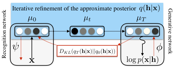
Figure 1: Iterative refinement for variational inference. An initial estimate of the variational parameters is made through a recognition network. The variational parameters are then updated iteratively, maximizing the lowerbound. The final approximate posterior is used to train the generative model by sampling. The recognition network parameters are updated using the KL divergence between the refined posterior $q_{k}$ and the output of the recognition network $q_{0}$.

To address the above issues, iterative refinement for variational inference (IRVI) uses the recognition network as a preliminary guess of the posterior, then refines the posterior through iterative updates of the variational parameters. For the refinement step, IRVI uses a stochastic transition operator, $g(.)$, that maximizes the variational lowerbound.

An overview of IRVI is available in Figure 1. For the expectation (E)-step, we feed the observation $\mathbf{x}$ through the recognition network to get the initial parameters, $\boldsymbol{\mu}_{0}$, of the approximate posterior, $q_{0}(\mathbf{h}|\mathbf{x};\boldsymbol{\psi})$. We then refine $\boldsymbol{\mu}_{0}$ by applying $T$ updates to the variational parameters, $\boldsymbol{\mu}_{t+1}=g(\boldsymbol{\mu}_{t},\mathbf{x})$, iterating through $T$ parameterizations $\boldsymbol{\mu}_{1},\dots,\boldsymbol{\mu}_{T}$ of the approximate posterior $q_{t}(\mathbf{h}|\mathbf{x})$.

With the final set of parameters, $\boldsymbol{\mu}_{T}$, the gradient estimate of the recognition parameters $\boldsymbol{\psi}$ in the maximization (M)-step is taken w.r.t the negative exclusive KL divergence:

$$-\nabla_{\boldsymbol{\psi}}D_{KL}(q_{T}(\mathbf{h}|\mathbf{x})||q_{0}(\mathbf{h}|\mathbf{x};\boldsymbol{\psi}))\approx\frac{1}{K}\sum_{k=1}^{K}\nabla_{\boldsymbol{\psi}}\log q_{0}(\mathbf{h}^{(k)}|\mathbf{x};\boldsymbol{\psi}),$$ (6)

where $\mathbf{h}^{(k)}\sim q_{T}(\mathbf{h}|\mathbf{x})$. Similarly, the gradients w.r.t. the parameters of the generative model $\boldsymbol{\phi}$ follow Eqs. (2) or (4) using samples from the refined posterior $q_{T}(\mathbf{h}|\mathbf{x})$. As an alternative to Eq. (6), we can maximize the negative inclusive KL divergence using the refined approximate posterior:

$$-\nabla_{\boldsymbol{\psi}}D_{KL}(p(\mathbf{h}|\mathbf{x})||q_{0}(\mathbf{h}|\mathbf{x};\boldsymbol{\psi}))\approx\sum_{k=1}^{K}\tilde{w}^{(k)}\nabla_{\boldsymbol{\psi}}\log q_{0}(\mathbf{h}^{(k)}|\mathbf{x};\boldsymbol{\psi}).$$ (7)

The form of the IRVI transition operator, $g(\boldsymbol{\mu}_{t},\mathbf{x})$, depends on the problem. In the case of continuous variables, we can make use of the VAE re-parameterization with the gradient of the lowerbound in Eq. (1) for our refinement step (see supplementary material). However, as this is not available with discrete units, we take a different approach that relies on adaptive importance sampling.

3.1 Adaptive Importance Refinement (AIR)

Adaptive importance sampling [AIS, 18] provides a general approach for iteratively refining the variational parameters. For Bernoulli distributions, we observe that the mean parameter of the true posterior, $\hat{\boldsymbol{\mu}}$, can be written as the expected value of the latent variables:

$$\hat{\boldsymbol{\mu}}=\mathbb{E}_{p(\mathbf{h}|\mathbf{x})}\left[\mathbf{h}\right]=\sum_{\mathbf{h}}\mathbf{h}\ p(\mathbf{h}|\mathbf{x})=\frac{1}{p(\mathbf{x})}\sum_{\mathbf{h}}q(\mathbf{h}|\mathbf{x})\ \mathbf{h}\ \frac{p(\mathbf{x},\mathbf{h})}{q(\mathbf{h}|\mathbf{x})}\approx\sum_{k=1}^{K}\tilde{w}^{(k)}\mathbf{h}^{(k)}.$$ (8)

As the initial estimator typically has high variance, AIS iteratively moves $\boldsymbol{\mu}_{t}$ toward $\hat{\boldsymbol{\mu}}$ by applying Eq. 8 until a stopping criteria is met. While using the update, $g(\boldsymbol{\mu}_{t},\mathbf{x},\gamma)=\sum_{k=1}^{K}\tilde{w}^{(k)}\mathbf{h}^{(k)}$ in principle works, a convex combination of importance sample estimate of the current step and the parameters from the previous step tends to be more stable:

$$\mathbf{h}^{(m)}\sim\text{Bernoulli}(\boldsymbol{\mu}_{k});\quad\boldsymbol{\mu}_{t+1}=g(\boldsymbol{\mu}_{t},\mathbf{x},\gamma)=(1-\gamma)\boldsymbol{\mu}_{t}+\gamma\sum_{k=1}^{K}\tilde{w}^{(k)}\mathbf{h}^{(k)}.$$ (9)

Here, $\gamma$ is the inference rate and $(1-\gamma)$ can be thought of as the adaptive “damping” rate. This approach, which we call adaptive importance refinement (AIR), should work with any discrete parametric distribution. Although AIR is applicable with continuous Gaussian variables, which model second-order statistics, we leave adapting AIR to continuous latent variables for future work.

3.2 Algorithm and Complexity

The general AIR algorithm follows Algorithm 1 with gradient variations following Eqs. (2), (4), (6), and (7). While iterative refinement may reduce the variance of stochastic gradient estimates and speed up learning, it comes at a computational cost, as each update is $T$ times more expensive than fixed approximations. However, in addition to potential learning benefits, AIR can also improve the approximate posterior of an already trained directed belief networks at test, independent on how the model was trained. Our implementation following Algorithm 1 is available at https://github.com/rdevon/IRVI.

Algorithm 1 AIR

0:  A generative model $p(\mathbf{x},\mathbf{h};\boldsymbol{\phi})=p(\mathbf{x}|\mathbf{h};\boldsymbol{\phi})p(\mathbf{h};\boldsymbol{\phi})$ and a recognition network $\boldsymbol{\mu}_{0}=f(\mathbf{x};\boldsymbol{\psi})$

0:  A transition operator $g(\mu,\mathbf{x},\gamma)$ and inference rate $\gamma$.

  Compute $\boldsymbol{\mu}_{0}=f(\mathbf{x};\boldsymbol{\psi})$ for $q_{0}(\mathbf{h}|\mathbf{x};\boldsymbol{\psi})$

  for t=1:T do

     Draw $K$ samples $\mathbf{h}^{(k)}\sim q_{t}(\mathbf{h}|\mathbf{x})$ and compute normalized importance weights $\tilde{w}^{(k)}$

     $\boldsymbol{\mu}_{t}=(1-\gamma)\boldsymbol{\mu}_{t-1}+\gamma\sum_{k=1}^{K}\tilde{w}^{(k)}\mathbf{h}^{(k)}$

  end for

  if reweight then

     $\Delta\boldsymbol{\phi}\propto\sum_{k=1}^{K}\tilde{w}^{(k)}\nabla_{\boldsymbol{\phi}}\log p(\mathbf{x},\mathbf{h}^{(k)};\boldsymbol{\phi})$

  else

     $\Delta\boldsymbol{\phi}\propto\frac{1}{K}\sum_{k=1}^{K}\nabla_{\boldsymbol{\phi}}\log p(\mathbf{x},\mathbf{h}^{(k)};\boldsymbol{\phi})$

  end if

  if inclusive KL Divergence then

     $\Delta\boldsymbol{\psi}\propto\sum_{k=1}^{K}\tilde{w}^{(k)}\nabla_{\boldsymbol{\psi}}\log q_{0}(\mathbf{h}^{(k)}|\mathbf{x};\boldsymbol{\psi})$

  else

     $\Delta\boldsymbol{\psi}\propto\frac{1}{K}\sum_{k=1}^{K}\nabla_{\boldsymbol{\psi}}\log q_{0}(\mathbf{h}^{(k)}|\mathbf{x};\boldsymbol{\psi})$

  end if

4 Related Work

Adaptive importance refinement (AIR) trades computation for expressiveness and is similar in this regard to the refinement procedure of hybrid MCMC for variational inference [HVI, 25] and normalizing flows for VAE [NF, 22]. HVI has a similar complexity as AIR, as it requires re-estimating the lowerbound at every step. While NF can be less expensive than AIR, both HVI and NF rely on the VAE re-parameterization to work, and thus cannot be applied to discrete variables. Sequential importance sampling [SIS, 6] can offer a better refinement step than AIS but typically requires resampling to control variance. While parametric versions exist that could be applicable to training directed graphical models with discrete units [9, 19], their applicability as a general refinement procedure is limited as the refinement parameters need to be learned.

Importance sampling is central to reweighted wake-sleep [RWS, 1], importance-weighted autoencoders [IWAE, 3], variational inference for Monte Carlo objectives [VIMCO, 15], and recent work on stochastic feed-forward networks [SFFN, 27, 20]. While each of these methods are competitive, they rely on importance samples from the recognition network and do not offer the low-variance estimates available from AIR. Neural variational inference and learning [NVIL, 14] is a single-sample and biased version of VIMCO, which is greatly outperformed by techniques that use importance sampling. Both NVIL and VIMCO reduce the variance of the Monte Carlo estimates of gradients by using an input-dependent baseline, but this approach does not necessarily provide a better posterior and cannot be used to give better estimates of the likelihood function or expectations.

Finally, IRVI is meant to be a general approach to refining the approximate posterior. IRVI is not limited to the refinement step provided by AIR, and many different types of refinement steps are available to improve the posterior for models above (see supplementary material for the continuous case). SIS and sequential importance resampling [SIR, 7] can be used as an alternative to AIR and may provide a better refinement step for IRVI.

5 Experiments

We evaluate iterative refinement for variational inference (IRVI) using adaptive importance refinement (AIR) for both training and evaluating directed belief networks. We train and test on the following benchmarks: the binarized MNIST handwritten digit dataset [24] and the Caltech-101 Silhouettes dataset. We centered the MNIST and Caltech datasets by subtracting the mean-image over the training set when used as input to the recognition network. We also train additional models using the re-weighted wake-sleep algorithm [RWS, 1], the state of the art for many configurations of directed belief networks with discrete variables on these datasets for comparison and to demonstrate improving the approximate posteriors with refinement. With our experiments, we show that 1) IRVI can train a variety of directed models as well or better than existing methods, 2) the gains from refinement improves the approximate posterior, and can be applied to models trained by other algorithms, and 3) IRVI can be used to improve a model with a relatively simple approximate posterior.

Models were trained using the RMSprop algorithm [11] with a batch size of $100$ and early stopping by recorded best variational lower bound on the validation dataset. For AIR, $20$ “inference steps" ($K=20$), $20$ adaptive samples ($M=20$), and an adaptive damping rate, $(1-\gamma)$, of $0.9$ were used during inference, chosen from validation in initial experiments. $20$ posterior samples ($N=20$) were used for model parameter updates for both AIR and RWS. All models were trained for $500$ epochs and were fine-tuned for an additional $500$ with a decaying learning rate and SGD.

We use a generative model composed of a) a factorized Bernoulli prior as with sigmoid belief networks (SBNs) or b) an autoregressive prior, as in published MNIST results with deep autoregressive networks [DARN, 8]:

$$\text{a)}\ p(\mathbf{h})=\prod_{i}p(h_{i});P(h_{i}=1)=\sigma(b_{i}),\quad\text{b)}\ P(h_{i}=1)=\sigma(\sum_{j=0}^{i-1}(W_{r}^{i,j<i}h_{j<i})+b_{i}),$$ (10)

where $\sigma$ is the sigmoid ($\sigma(x)=1/(1+\exp(-x))$) function, $W_{r}$ is a lower-triangular square matrix, and $\mathbf{b}$ is the bias vector.

For our experiments, we use conditional and approximate posterior densities that follow Bernoulli distributions:

$$P(h_{i,l}=1|\mathbf{h}_{l+1})=\sigma(W_{l}^{i,:}\cdot\mathbf{h}_{l+1}+b_{i,l}),$$ (11)

where $W_{l}$ is a weight matrix between the $l$ and $l+1$ layers. As in Gregor et al. [8] with MNIST, we do not use autoregression on the observations, $\mathbf{x}$, and use a fully factorized approximate posterior.

5.1 Variance Reduction and Choosing the AIR Objective

Figure 2: The log-likelihood (left) and normalized effective sample size (right) with epochs in log-scale on the training set for AIR with $5$ and $20$ refinement steps (vanilla AIR), reweighted AIR with $5$ and $20$ refinement steps, reweighted AIR with inclusive KL objective and $5$ or $20$ refinement steps, and reweighted wake-sleep (RWS), all with a single stochastic latent layer. All models were evaluated with $100$ posterior samples, their respective number of refinement steps for the effective sample size (ESS), and with $20$ refinement steps of AIR for the log-likelihood. Despite longer wall-clock time per epoch,

The effective sample size (ESS) in Eq. (5) is a good indicator of the variance of gradient estimate. In Fig. 5 (right), we observe that the ESS improves as we take more AIR steps when training a deep belief network (AIR(5) vs AIR(20)). When the approximate posterior is not refined (RWS), the ESS stays low throughout training, eventually resulting in a worse model. This improved ESS reveals itself as faster convergence in terms of the exact log-likelihood in the left panel of Fig. 5 (see the progress of each curve until 100 epochs. See also supplementary materials for wall-clock time.)

This faster convergence does not guarantee a good final log-likelihood, as the latter depends on the tightness of the lowerbound rather than the variance of its estimate. This is most apparent when comparing AIR(5), AIR+RW(5) and AIR+RW+IKL(5). AIR(5) has a low variance (high ESS) but computes the gradient of a looser lowerbound from Eq. (2), while the other two compute the gradient of a tighter lowerbound from Eq. (4). This results in AIR(5) converging faster than the other two, while the final log-likelihood estimates are better for the other two.

We however observe that the final log-likelihood estimates are comparable across all three variants (AIR, AIR+RW and AIR+RW+IKL) when a sufficient number of AIR steps are taken so that $\mathcal{L}_{1}$ is sufficiently tight. When 20 steps were taken, we observe that the AIR(20) converges faster as well as achieves a better log-likelihood compared to AIR+RW(20) and AIR+RW+IKL(20). Based on these observations, we use vanilla AIR (subsequently just “AIR”) in our following experiments.

5.2 Training and Density Estimation

We evaluate AIR for training SBNs with one, two, and three layers of $200$ hidden units and DARN with $200$ and $500$ hidden units, comparing against our implementation of RWS. All models were tested using $100,000$ posterior samples to estimate the lowerbounds and average test log-probabilities.

When training SBNs with AIR and RWS, we used a completely deterministic network for the approximate posterior. For example, for a 2-layer SBN, the approximate posterior factors into the approximate posteriors for the top and the bottom hidden layers, and the initial variational parameters of the top layer, $\boldsymbol{\mu}^{(2)}_{0}$ are a function of the initial variational parameters of the first layer, $\boldsymbol{\mu}^{(1)}_{0}$:

$$q_{0}(\mathbf{h}_{1},\mathbf{h}_{2}|\mathbf{x})=q_{0}(\mathbf{h}_{1}|\mathbf{x};\boldsymbol{\mu}^{(1)}_{0})q(\mathbf{h}_{2}|\mathbf{x};\boldsymbol{\mu}^{(2)}_{0});\quad\boldsymbol{\mu}^{(1)}_{0}=f_{1}(\mathbf{x};\boldsymbol{\psi}_{1});\quad\boldsymbol{\mu}^{(2)}_{0}=f_{2}(\boldsymbol{\mu}^{(1)}_{0};\boldsymbol{\psi}_{2}).$$ (12)

For DARN, we trained two different configurations on MNIST: one with $500$ stochastic units and an additional hyperbolic tangent deterministic layer with $500$ units in both the generative and recognition networks, and another with $200$ stochastic units with a $500$ hyperbolic tangent deterministic layer in the generative network only. We used DARN with $200$ units with the Caltech-101 silhouettes dataset.

Table 1: Results for adaptive importance sampling iterative refinement (AIR), reweighted wake-sleep (RWS), and RWS with refinement with AIR at test (RWS+) for a variety of model configurations. Additional sigmoid belief networks (SBNs) trained with neural variational inference and learning (NVIL) from †Mnih and Gregor [14] and variational inference for Monte Carlo objectives (VIMCO) from §Mnih and Rezende [15]. AIR is trained with $20$ inference steps and adaptive samples ($K=20,M=20$) in training (*3 layer SBN was trained with $50$ steps with a inference rate of $0.05$). NVIL DARN results are from fDARN and VIMCO was trained using $50$ posterior samples (as opposed to $20$ with AIR and RWS).

Model	MNIST					Caltech-101 Silhouettes
	RWS	RWS+	AIR	NVIL†	VIMCO§	RWS	RWS+	AIR
SBN 200	102.51	102.00	100.92	113.1	–	121.38	118.63	116.61
SBN 200-200	93.82	92.83	92.90	99.8	–	112.86	107.20	106.94
SBN 200-200-200	92.00	91.02	$\text{92.56}^{*}$	96.7	90.9§	110.57	104.54	104.36
DARN 200	86.91	86.21	85.89	92.5†	–	113.69	109.73	109.76
DARN 500	85.40	84.71	85.46	90.7†	–	–	–	–

The results of our experiments with the MNIST and Caltech-101 silhouettes datasets trained with AIR, RWS, and RWS refined at test with AIR (RWS+) are in Table 1. Refinement at test (RWS+) always improves the results for RWS. As our unrefined results are comparable to those found in Bornschein and Bengio [1], the improved results indicate many evaluations of Helmholtz machines in the literature could benefit from refinement with AIR to improve evaluation accuracy. For most model configurations, AIR and RWS perform comparably, though RWS appears to do better in the average test log-probability estimates for some configurations of MNIST. RWS+ performs comparably with variational inference for Monte Carlo objectives [VIMCO, 15], despite the reported VIMCO results relying on more posterior samples in training. Finally, AIR results approach SOTA with Caltech-101 silhouettes with 3-layer SBNs against neural autoregressive distribution estimator [NADE, 1].

We also tested our log-probability estimates against the exact log-probability (by marginalizing over the joint) of smaller single-layer SBNs with $20$ stochastic units. The exact log-probability was $-127.474$ and our estimate with the unrefined approximate was $-127.51$ and $-127.48$ with $100$ refinement steps. Overall, this result is consistent with those of Table 1, that iterative refinement improves the accuracy of log-probability estimates.

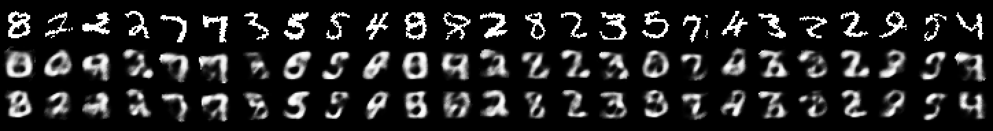
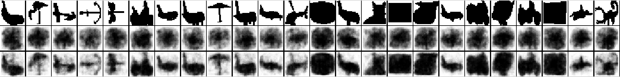
Figure 3: Top: Average reconstructions, $1/N\sum_{n=1}^{N}p(\mathbf{x}|\mathbf{h}^{(n)})$, for $\mathbf{h}^{(n)}$ sampled from the output of the recognition network, $q_{0}(\mathbf{h}|\mathbf{x})$ (middle row) against those sampled from the refined posterior, $q_{T}(\mathbf{h}|\mathbf{x})$ (bottom row) for $T=20$ with a model trained on MNIST. Top row is ground truth. Among the digits whose reconstruction changes the most, many changes correctly reveal the identity of the digit. Bottom: Average reconstructions for a single-layer model with $200$ trained on Caltech-101 silhouettes. Instead of using the posterior from the recognition network, we derived a simpler version, setting $80\%$ of the variational parameters from the recognition network to $0.5$, then applied iterative refinement.

5.3 Posterior Improvement

In order to visualize the improvements due to refinement and to demonstrate AIR as a general means of improvement for directed models at test, we generate $N$ samples from the approximate posterior without ($\mathbf{h}\sim q_{0}(\mathbf{h}|\mathbf{x};\boldsymbol{\psi})$) and with refinement ($\mathbf{h}\sim q_{T}(\mathbf{h}|\mathbf{x})$), from a single-layer SBN with $20$ stochastic units originally trained with RWS. We then use the samples from the approximate posterior to compute the expected conditional probability or average reconstruction: $\frac{1}{N}\sum_{n=1}^{N}p(\mathbf{x}|\mathbf{h}^{(n)})$. We used a restricted model with a lower number of stochastic units to demonstrate that refinement also works well with simple models, where the recognition network is more likely to “average” over latent configurations, giving a misleading evaluation of the model’s generative capability.

We also refine the approximate posterior of a simplified version of the recognition network of a single-layer SBN with $200$ units trained with RWS. We simplified the approximate posterior by first computing $\boldsymbol{\mu}_{0}=f(\mathbf{x};\boldsymbol{\psi})$, then randomly setting $80\%$ of the variational parameters to $0.5$.

Fig. 3 shows improvement from refinement for $25$ digits from the MNIST test dataset, where the samples chosen were those of which the expected reconstruction error of the original test sample was the most improved. The digits generated from the refined posterior are of higher quality, and in many cases the correct digit class is revealed. This shows that, in many cases where the recognition network indicates that the generative model cannot model a test sample correctly, refinement can more accurately reveal the model’s capacity. With the simplified approximate posterior, refinement is able to retrieve most of the shape of images from the Caltech-101 silhouettes, despite only starting with $20\%$ of the original parameters from the recognition network. This indicates that the work of inference need not all be done via a complex recognition network: iterative refinement can be used to aid in inference with a relatively simple approximate posterior.

6 Conclusion

We have introduced iterative refinement for variational inference (IRVI), a simple, yet effective and flexible approach for training and evaluating directed belief networks that works by improving the approximate posterior from a recognition network. We demonstrated IRVI using adaptive importance refinement (AIR), which uses importance sampling at each iterative step, and showed that AIR can be used to provide low-variance gradients to efficiently train deep directed graphical models. AIR can also be used to more accurately reveal the generative model’s capacity, which is evident when the approximate posterior is of poor quality. The improved approximate posterior provided by AIR shows an increased effective samples size, which is a consequence of a better approximation of the true posterior and improves the accuracy of the test log-probability estimates.

7 Acknowledgements

This work was supported by Microsoft Research to RDH (internship under NJ); NIH P20GM103472, R01 grant REB020407, and NSF grant 1539067 to VDC; and ONR grant N000141512791 and ADeLAIDE grant FA8750-16C-0130-001 to RS. KC was supported in part by Facebook, Google (Google Faculty Award 2016) and NVidia (GPU Center of Excellence 2015-2016), and RDH was supported in part by PIBBS.

8 Supplementary material

8.1 Continuous Variables

With variational autoencoders (VAE), the back-propagated gradient of the lowerbound with respect to the approximate posterior is composed of individual gradients for each factor, $\mu_{i}$ that can be applied simultaneously. Applying the gradient directly to the variational parameters, $\boldsymbol{\mu}$, without back-propagating to the recognition network parameters, $\boldsymbol{\psi}$, yields a simple iterative refinement operator:

$$\boldsymbol{\mu}_{t+1}=g(\boldsymbol{\mu}_{t},\mathbf{x},\gamma)=\boldsymbol{\mu}_{t}+\gamma\nabla_{\boldsymbol{\mu}}\mathcal{L}_{1}(\boldsymbol{\mu},\mathbf{x},\boldsymbol{\epsilon}),$$ (13)

where $\gamma$ is the inference rate hyperparameter and $\boldsymbol{\epsilon}$ is auxiliary noise used in the re-parameterization.

This gradient-descent iterative refinement (GDIR) is very straightforward with continuous latent variables as with VAE. However, GDIR with discrete units suffers the same shortcomings as when passing the gradients directly, so a better transition operator is needed (AIR).

In the limit of $T=0$, we do not arrive at VAE, as the gradients are never passed through the approximate posterior during learning. However, as the complete computational graph involves a series of differentiable variables, $\boldsymbol{\mu}_{t}$, in addition to auxiliary noise, it is possible to pass gradients through GDIR to the recognition network parameters, $\boldsymbol{\psi}$, during learning, though we do not here.

For continuous latent variables, we used the same network structure as in [13, 25]. Results for GDIR are presented in Table 2 for the MNIST dataset, and included for comparison are methods for learning non-factorial latent distributions for Gaussian variables and the corresponding result for VAE, the baseline.

Table 2: Lowerbounds and NLL for various continuous latent variable models and training algorithms along with the corresponding VAE estimates. We use $200$ latent Gaussian variables. †From Salimans et al. [25]. §From Rezende and Mohamed [22]. ‡From Burda et al. [3].

Model	$\leq$ -log p(x)	$\approx$ -log p(x)
VAE	94.48	89.31
VAE (w/ refinement)	90.57	88.53
$\text{GDIR}_{50,20}$	90.60	88.54
VAE†	94.18	88.95
$\text{HVI}_{1}$†	91.70	88.08
$\text{HVI}_{8}$†	88.30	85.51
VAE §	89.9
$\text{DLGM+NF}_{80}$ §	85.1
VAE‡		86.35
IWAE ($K=50$)‡		84.78

Though GDIR can improve the posterior in VAE, our results show that VAE is at an upper-bound for learning with a factorized posterior on the MNIST dataset. Further improvements on this dataset must be made by using a non-factorized posterior (re-weighting or sequential Monte Carlo with importance weighting). GDIR may still also provide improvement for training models with other datasets, and we leave this for future work.

9 Refinement of the lowerbound and effective sample size

Figure 4: The variational lowerbound (left) and normalized effective sample size (ESS, right) the test set as the posterior is refined from the initial posterior provided by the recognition network. Models were trained with AIR with $20$ refinement steps and one (AIR 200), two (AIR 200x2), and three (AIR 200x3) hidden layers. Refinement shows clear improves of both the variational lowerbound and effective sample size.

Iterative refinement via adaptive inference refinement (AIR) improves the variational lowerbound and effective sample size (ESS) of the approximate posterior. To show this, we trained models with one, two, and three hidden layers with $200$ binary units trained using AIR with $20$ inference steps on the MNIST dataset for $500$ epochs. Taking the initial approximate posterior from each model, we refined the posterior up to $50$ steps (Figure 4), evaluating the lowerbound and ESS using $100$ posterior samples. Refinement improves the posterior from models trained on AIR well beyond the number of steps used in training.

10 Updates and wall-clock times

Figure 5: The log-likelihood (left) and normalized effective sample size (right) with epochs in log-scale on the training set for AIR with $5$ and $20$ refinement steps (vanilla AIR), reweighted AIR with $5$ and $20$ refinement steps, reweighted AIR with inclusive KL objective and $5$ or $20$ refinement steps, and reweighted wake-sleep (RWS). Despite longer wall-clock time per epoch, AIR converges to lower log-likelihoods and effective sample size (ESS) than RWS.

Figure 6: Negative lowerbound and effective samples size (ESS) across updates (epochs) and wall-clock time (seconds) for two and three layer sigmoid belief networks trained with adaptive iterative refinement (AIR) and reweighted wake-sleep (RWS). AIR was trained with $20$ refinement steps with a damping rate of $\gamma=0.9$. Each model was trained for $500$ epochs and evaluated on the training dataset using $100$ posterior samples. AIR takes less updates to reach equivalent variational lowerbound and ESS than RWS. While RWS can reach a higher lowerbound at earlier wall-clock times, AIR and RWS appear to converge to the same value, and AIR reaches much higher ESS.

Adaptive iterative refinement (AIR) and reweighted wake-sleep [RWS, 1] have competing convergence wall-clock times, while AIR outperforms on updates (Figures 5 and 6). AIR converges to a higher lowerbound and with far fewer updates than RWS, though RWS converges sooner to a similar value as AIR does later in training time. AIR outperforms RWS in ESS in both wall-clock time and updates. For a more accurate comparison, RWS may need to be trained at wall-clock times equal to that afforded to AIR. However, these results support the conclusion that AIR converges to similar values as RWS in less updates but similar wall-clock times.

11 Bidirectional Helmholtz machines and AIR

As an alternative to the variational lowerbound, a lowerbound can be formulated from the geometric mean of the joint generative and approximate posterior models:

$$p^{\star}(\mathbf{x},\mathbf{h})=\frac{1}{Z}\sqrt{p(\mathbf{x},\mathbf{h})q(\mathbf{x},\mathbf{h})}.$$ (14)

In this procedure, known as bidirectional Helmholtz machines [2], the lowerbound, which minimizes the Bhattacharyya distance ($D_{B}(p,q)=-\log\sum_{y}\sqrt{p(y)q(y)}$), yields estimates of the likelihood, $p^{\star}(\mathbf{x})$, with importance weights,

$$w^{(k)}=\sqrt{\frac{p(\mathbf{x},\mathbf{h}^{(k)})}{q(\mathbf{h}^{(k)}|\mathbf{x})}}.$$ (15)

Similar to with the variational lowerbound, we can refine the approximate posterior to maximize this lowerbound by simply replacing the weights in Equation 15.

We performed similar experiments to those as the experiments on wall-clock times above, using only a three layer SBN trained for $500$ epochs with the equivalent AIR and BiHM procedures using the bidirectional lowerbound importance weights. We evaluated these models using $10000$ posterior samples on the test dataset and evaluated BiHM with (BiHM+) and without refinement.

Our results show similar negative log likelihoods for AIR ($92.40$ nats), BiHM ($93.30$ nats), and BiHM+ ($92.90$ nats), though AIR slightly outperforms BiHM+, and BiHM+ slightly outperforms BiHM. Further optimization is necessary for a better comparison to our experiments with the variational lowerbound. However these observations are consistent with those from our original experiments: AIR can be used to improve the posterior both in training and when evaluating models, regardless of how they were trained. Furthermore, AIR is compatible with optimizations based on alternative lowerbounds, broadening the scope in which AIR is applicable.

References

- Bornschein and Bengio [2014] Jörg Bornschein and Yoshua Bengio. Reweighted wake-sleep. arXiv preprint arXiv:1406.2751, 2014.
- Bornschein et al. [2015] Jorg Bornschein, Samira Shabanian, Asja Fischer, and Yoshua Bengio. Bidirectional helmholtz machines. arXiv preprint arXiv:1506.03877, 2015.
- Burda et al. [2015] Yuri Burda, Roger Grosse, and Ruslan Salakhutdinov. Importance weighted autoencoders. arXiv preprint arXiv:1509.00519, 2015.
- Dayan et al. [1995] Peter Dayan, Geoffrey E Hinton, Radford M Neal, and Richard S Zemel. The helmholtz machine. Neural computation, 7(5):889–904, 1995.
- Dempster et al. [1977] Arthur P Dempster, Nan M Laird, and Donald B Rubin. Maximum likelihood from incomplete data via the em algorithm. Journal of the royal statistical society. Series B (methodological), 1977.
- Doucet et al. [2001] Arnaud Doucet, Nando De Freitas, and Neil Gordon. An introduction to sequential monte carlo methods. In Sequential Monte Carlo methods in practice, pages 3–14. Springer, 2001.
- Gordon et al. [1993] Neil J Gordon, David J Salmond, and Adrian FM Smith. Novel approach to nonlinear/non-gaussian bayesian state estimation. In Radar and Signal Processing, IEE Proceedings F, volume 140, pages 107–113. IET, 1993.
- Gregor et al. [2013] Karol Gregor, Ivo Danihelka, Andriy Mnih, Charles Blundell, and Daan Wierstra. Deep autoregressive networks. arXiv preprint arXiv:1310.8499, 2013.
- Gu et al. [2015a] Shixiang Gu, Zoubin Ghahramani, and Richard E Turner. Neural adaptive sequential monte carlo. In Advances in Neural Information Processing Systems, pages 2611–2619, 2015a.
- Gu et al. [2015b] Shixiang Gu, Sergey Levine, Ilya Sutskever, and Andriy Mnih. Muprop: Unbiased backpropagation for stochastic neural networks. arXiv preprint arXiv:1511.05176, 2015b.
- Hinton [2012] Geoffrey Hinton. Neural networks for machine learning. Coursera, video lectures, 2012.
- Hinton et al. [2006] Geoffrey E Hinton, Simon Osindero, and Yee-Whye Teh. A fast learning algorithm for deep belief nets. Neural computation, 18(7):1527–1554, 2006.
- Kingma and Welling [2013] Diederik Kingma and Max Welling. Auto-encoding variational bayes. arXiv preprint arXiv:1312.6114, 2013.
- Mnih and Gregor [2014] Andriy Mnih and Karol Gregor. Neural variational inference and learning in belief networks. In Proceedings of the 31st International Conference on Machine Learning (ICML-14), pages 1791–1799, 2014.
- Mnih and Rezende [2016] Andriy Mnih and Danilo J Rezende. Variational inference for monte carlo objectives. arXiv preprint arXiv:1602.06725, 2016.
- Neal [1992] Radford M Neal. Connectionist learning of belief networks. Artificial intelligence, 56(1), 1992.
- Neal and Hinton [1998] Radford M Neal and Geoffrey E Hinton. A view of the em algorithm that justifies incremental, sparse, and other variants. In Learning in graphical models, pages 355–368. Springer, 1998.
- Oh and Berger [1992] Man-Suk Oh and James O Berger. Adaptive importance sampling in monte carlo integration. Journal of Statistical Computation and Simulation, 41(3-4):143–168, 1992.
- Paige and Wood [2016] Brooks Paige and Frank Wood. Inference networks for sequential monte carlo in graphical models. arXiv preprint arXiv:1602.06701, 2016.
- Raiko et al. [2014] Tapani Raiko, Mathias Berglund, Guillaume Alain, and Laurent Dinh. Techniques for learning binary stochastic feedforward neural networks. arXiv preprint arXiv:1406.2989, 2014.
- Rezende et al. [2014] Danilo J Rezende, Shakir Mohamed, and Daan Wierstra. Stochastic backpropagation and approximate inference in deep generative models. In Proceedings of the 31st International Conference on Machine Learning (ICML-14), pages 1278–1286, 2014.
- Rezende and Mohamed [2015] Danilo Jimenez Rezende and Shakir Mohamed. Variational inference with normalizing flows. arXiv preprint arXiv:1505.05770, 2015.
- Salakhutdinov and Larochelle [2010] Ruslan Salakhutdinov and Hugo Larochelle. Efficient learning of deep boltzmann machines. In International Conference on Artificial Intelligence and Statistics, pages 693–700, 2010.
- Salakhutdinov and Murray [2008] Ruslan Salakhutdinov and Iain Murray. On the quantitative analysis of deep belief networks. In Proceedings of the 25th international conference on Machine learning, pages 872–879. ACM, 2008.
- Salimans et al. [2015] Tim Salimans, Diederik Kingma, and Max Welling. Markov chain monte carlo and variational inference: Bridging the gap. In David Blei and Francis Bach, editors, Proceedings of the 32nd International Conference on Machine Learning (ICML-15), pages 1218–1226. JMLR Workshop and Conference Proceedings, 2015. URL http://jmlr.org/proceedings/papers/v37/salimans15.pdf.
- Saul et al. [1996] Lawrence K Saul, Tommi Jaakkola, and Michael I Jordan. Mean field theory for sigmoid belief networks. Journal of artificial intelligence research, 4(1):61–76, 1996.
- Tang and Salakhutdinov [2013] Yichuan Tang and Ruslan R Salakhutdinov. Learning stochastic feedforward neural networks. In Advances in Neural Information Processing Systems, pages 530–538, 2013.